Abstract
Drinking water systems’ energy footprints depend mostly on the source, quality, and volume of water supply, but also on local temperature and precipitation, both of which are changing with the global climate. From a previous survey, we develop an equation for modeling relative changes in U.S. water utilities’ annual energy use, in which their energy use increases with temperature and decreases with precipitation. To demonstrate, we insert gridded projections from three scenarios in the EPA’s Climate Resilience Evaluation and Awareness Tool (CREAT) and compare 2035 and 2060 periods with a 1981–2010 baseline. Averaged over the continental United States, the 2060 central scenario projects 2.7 °C warmer temperatures and 2.9 cm more annual precipitation. For the same water demand, we estimate that these conditions will cause U.S. water systems’ energy use to change by −0.7% to 13.7% depending on the location (average 8.5% across all grid cells). Warming accounts for a general increase, and local changes in precipitation can add to or subtract from it. We present maps showing the spatial variability for each scenario. Water systems are essential infrastructure that support sustainable communities, and the analysis underscores their needs for energy management, renewable energy, water conservation, and climate change resilience.
1. Introduction
Twenty years ago, Levin et al. [1] reviewed the research and cautioned that a warming global climate may lead to several problems affecting drinking water supply. Among them were higher microbial and nutrient loadings, earlier snowmelt, more frequent harmful algal blooms, and greater water demand and water stress. Since then, the warming climate has been well documented [2] and numerous studies have confirmed the impacts on water systems. Much guidance [3,4,5,6,7,8,9] has also appeared, describing how water systems should adapt to the new climate conditions.
While many aspects of this research space have been well explored, one question that has received less attention is how climate change will affect water systems’ energy use. Water systems need energy to extract, pump, treat, and distribute water with sufficient quality and pressure to end users [10,11,12,13,14,15,16], which is just one facet of the broader water–energy nexus [17,18]. A changing climate may alter water availability, water quality, and other factors that, even for the same water demand, will lead to changes in energy use.
Past studies have showed how water systems’ energy footprints correlate with climate variables. Rothausen and Conway [14] suggested that water systems’ energy use is likely to increase because of climate change and other factors. Globally, the most energy-intensive water systems are located in places with lower average precipitation [11]. Sowby and Burian’s [19] model of U.S. water systems showed that their energy use increases with temperature and decreases with precipitation. Similarly, a negative correlation between precipitation and energy use in Denver’s water supply over 20 years has been observed (R. B. Sowby and A. Capener, manuscript under review). Energy use at water and wastewater treatment plants increases with heating degree days [20,21]. However, none of these studies have explicitly linked climate change to water systems’ energy footprints in a quantitative way.
One exception is a study by Mo et al. [22], who analyzed one U.S. water treatment plant in depth, forecasting its future energy use as a function of climate scenarios and water-quality variables. They projected a 3–6% decrease in energy intensity (energy use per volume of water) for their particular case, but they concluded that the effects could vary significantly by geographic location. Similarly, Stang et al. [23] compared two U.S. plants under projected climate scenarios and found mixed changes in their energy footprints. The outcomes of both studies suggest that if many water systems are to be evaluated at once, a geographically sensitive approach is necessary.
How will U.S. water systems’ energy footprints increase or decrease with climate change? To answer this question, we (1) propose a method for estimating relative changes in energy use based on an existing regression model of U.S. water systems and (2) estimate relative energy changes using the new method and data from the U.S. Environmental Protection Agency (EPA). We then discuss implications for water system planning.
2. Materials and Methods
2.1. Water System Energy Model
From a dataset of over 100 U.S. water systems [15,24,25], Sowby and Burian [19] developed and validated a regression model for a water system’s annual energy use, (kWh):
or
where is the annual water use (m3), is an indicator (0 or 1) of gravity-fed surface water supply, is an indicator (0 or 1) of imported water supply, is the average annual air temperature (°C), and is the average annual precipitation (cm). The positive and negative signs of the temperature and precipitation coefficients are logical; warmer or drier conditions make water less readily available, so extra energy must be expended to obtain it. Consider, for example, a water treatment plant that pumps water from a lake; low precipitation reduces runoff into the lake and warm temperatures increase evaporation from the lake, so the lake level falls, and the plant must use more energy to pump the greater distance. Only energy use in the operational phase is of interest, as energy use during construction and end-of-life is insignificant in the overall profile [12,26,27].
While the expression was designed for characterizing energy footprints across multiple water utilities in a single time period, we see its potential for estimating their energy use deviations associated with climate change. Precipitation and temperature are already embedded in the expression, and a comparison of two time periods will yield the change of interest. For the purposes of climate analysis, we assume the first four terms in the exponent of Equation (2) are constant properties of the water system and replace them with a single term . That is, we are not accounting for increasing or decreasing water consumption, loss of existing water sources, development of new water sources, or other internal factors. The expression then becomes
More than the absolute energy use, however, we seek the relative change in energy use between two time periods. As a ratio of two time periods, the constant cancels out:
We then define the temperature change and the precipitation change and substitute them into Equation (4):
Alternatively, we calculate the proportion of change in the energy use, , as:
Equations (5) and (6), as an innovative adaptation of Equation (1), say that relative to a water system’s baseline energy use, warmer conditions will increase energy use while wetter conditions will decrease energy use. It helps answer the question, “if the water system itself is held constant, how will its energy use change as a function of precipitation and temperature?”.
2.2. Applicability and Limitations
The method we have outlined is designed for studying incremental changes in a water system’s annual energy footprint due to trends in annual temperature and precipitation. It does not consider extreme events (e.g., drought, flood, disaster) or seasonal weather variations that fall outside the annual scope, nor does it consider population growth, water demand/conservation, new water sources or facilities, or other factors of the water system that were assumed to be fixed in the constant of Equations (3) and (4) but in reality may greatly affect energy use. Because such variables are specific to individual water systems and cannot be analyzed on a national scale, this was a necessary assumption to isolate the climate change effects (external) from the water supply effects (internal). The method is valid only in the continental United States, where the base data originated.
One limitation is the dataset used for the energy model of the foregoing equations, which is based on a short historical record, relative to the climate timescale in question. The challenges of acquiring large samples of energy-for-water panel data at utility-scale resolution are well documented [10,15,28,29]. While the model is the best available and showed good fit when it was developed, we acknowledge that its uncertainty increases farther into the future. We advise caution when using it for long-term projections and extreme climate scenarios because the results may be unreliable.
While the model is limited in these regards, it has several advantages. One is its simplicity and transparency, which lends itself to use by water practitioners and policy leaders. Another is its ability to isolate energy use changes attributable to temperature and precipitation rather than internal factors such as water demand. Furthermore, because the equation estimates relative ratios between two time periods rather than absolute energy use, the water system’s baseline energy use need not be known. The approach thus bypasses one of the major data challenges in energy-for-water studies [28,29]. It is also independent of climate models; projected changes in precipitation or temperature from any climate model and any time period may be entered into Equation (6). Repeating with multiple values for a single location enables scenario planning and representation of uncertainty; repeating across multiple locations enables cross-sectional and panel characterizations.
2.3. Climate Change Projections
To demonstrate the method, we insert data from climate projections and estimate the impact on water systems’ energy footprints in the continental United States. In this case, we take climate data from the Climate Resilience Evaluation and Awareness Tool (CREAT), an online resource in the EPA’s Creating Resilient Water Utilities (CRWU) program that helps water utilities evaluate climate-related risks [30]. While many climate datasets are available, CREAT is advantageous because it offers both a long-range forecast and hindcast, it is an authoritative EPA product, and U.S. water suppliers will be familiar with it. It offers downscaled, gridded data that cover the continental United States on a regular 0.5 degree grid, which is sufficient to capture spatially varying climates across the country.
The CREAT projections [31,32] are drawn from a 38-model ensemble of the Coupled Model Intercomparison Project Phase 5 (CMIP5) [33]. The ensemble assumes Representative Concentration Pathway (RCP) 8.5, which represents the highest carbon emissions of the CMIP5 scenarios (RCP2.6, RCP4.5, RCP6, and RCP8.5). Because CREAT is a preparedness tool for water utilities, its choice of RCP8.5 as the worst emissions case is deliberate. Forecasting so far into the future is inherently uncertain, hence the need for multiple models to project a range of possibilities in an ensemble. For planning purposes, CREAT defines three scenarios, as follows:
- Hot/Dry: Average of five models closest to 95th percentile of annual temperature projections and 5th percentile of annual precipitation projections.
- Central: Average of five models closest to 50th percentile of annual temperature projections and 50th percentile of annual precipitation projections.
- Warm/Wet: Average of five models closest to 5th percentile of annual temperature projections and 95th percentile of annual precipitation projections.
Projections are provided for the 2035 time period (2026–2045) and 2060 time period (2051–2070). Specifically, we use (1) projections of change in average annual temperature and precipitation, and (2) historical average annual precipitation for the period 1981–2010 [34]. Both datasets are needed because climate models give temperature change in degrees but precipitation change as percentages, requiring reference to the baseline precipitation in order to calculate the changes in terms of depth as needed for Equation (6). The precipitation depth change is calculated by multiplying the gridded precipitation percentage change forecast dataset by the gridded historical average precipitation dataset. The data are supplied in U.S. customary units, and we convert the data to metric units during processing. Figure 1 diagrams how each dataset is used with Equation (6) to calculate the percent energy use changes.
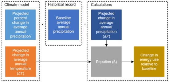
Figure 1.
Diagram of change in energy use calculations.
3. Results
3.1. Results Overview
Table 1 summarizes the projected changes in temperature, precipitation, and water system energy use for the three scenarios, averaged from the gridded CREAT data we analyzed over the continental United States. The results vary spatially; Figure 2 maps the temperature projections, Figure 3 maps the precipitation projections, and Figure 4 combines them (via Equation (6)) to map the projected changes in water system energy use. Figure 5 shows the ranges of energy use changes from Figure 4 as box-and-whisker plots.

Table 1.
Projected changes in temperature, precipitation, and water system energy use.
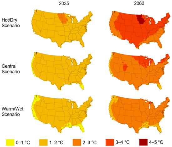
Figure 2.
Projected changes in average annual temperature.
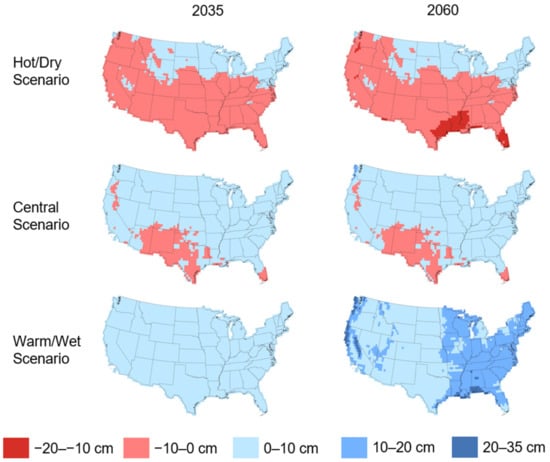
Figure 3.
Projected changes in average annual precipitation.
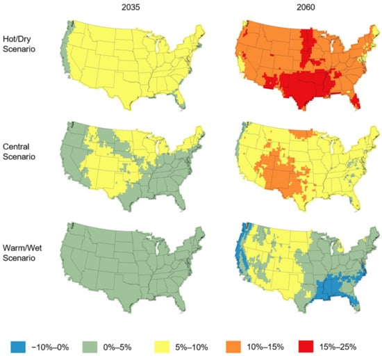
Figure 4.
Projected changes in annual water system energy use due to temperature and precipitation.
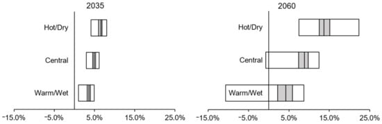
Figure 5.
Box-and-whisker plots of projected changes in annual water system energy use.
3.2. Temperature and Precipitation
Temperature (Figure 2) is projected to increase across all scenarios. Warming is most pronounced over the country’s interior and northern regions, especially in the 2060 scenarios. Precipitation (Figure 3) shows more variation by scenario. The 2060 hot/dry scenario shows less precipitation overall (−2.2 cm) but is divided between a wetter north and a drier south. The 2060 warm/wet scenario shows more precipitation overall (9.2 cm), especially in the east and along the Pacific and Gulf coasts. In the 2060 central scenario, precipitation increases by 2.9 cm overall but decreases in the southwest. It is interesting to note the north–south division of the hot/dry scenario and the east–west division of the warm/wet scenario as they concern projected precipitation changes; the central scenario is a combination of the two.
U.S. climate models are quite robust with regard to warming—most simulations agree on the direction of the temperature changes—but less robust with regard to precipitation, because of the variability in historic precipitation that makes some future changes less significant [35,36]. Our purpose is not to assess CREAT, but we trust the dataset because its projections for both temperature and precipitation generally agree with the Fourth National Climate Assessment [36] and also with more recent results for the United States from CMIP6 [35,37].
3.3. Water System Energy Use
Figure 4 combines the location-specific projected temperature and precipitation changes in Figure 2 and Figure 3 to estimate percent change in energy use for each grid cell in the CREAT forecasts using Equation (6). In the 2060 hot/dry scenario, the average energy increase is 13.7%, ranging from 7.5% along the east and west coasts to 22.3% in the south central states, where projected warming and drying coincide. In the 2060 central scenario, the average energy increase is 8.5%, with maximums (12.5%) occurring in a large hotspot over the southwest and some slight decreases (−0.7%) in wetter areas of the Pacific Northwest. In the 2060 warm/wet scenario, the east–west pattern appears again; precipitation becomes the dominant effect, offsetting some of the warming where the average energy increase is 3.6% and ranges from −10.7% on the wetter east coast, west coast, and Gulf coast to 8.7% in the general west.
To be clear, the averages, as in Table 1, are weighted equally in each grid cell, not by water system presence, size, population, or energy use. Nonetheless, the regions where energy use is expected to increase overlie the most populous parts of the country. We expect that, in practice, map users will look for individual locations of interest, and we provide GeoTIFFs in the Supplementary Materials for this purpose.
Two observations are apparent in Figure 5 (which uses the same data as Figure 4). Firstly, the energy use changes are greater in the hotter/drier scenarios. This is a direct implication of Equation (6) and the signs of its coefficients for temperature and precipitation. In the warm/wet scenario, as noted above, wetter conditions in some areas offset the increased energy use due to warming. Secondly, the energy use changes diverge with time. The changes are narrowly confined in the 2035 period but spread out considerably in the 2060 period as a consequence of the spatially diverse temperature and precipitation changes projected in the later future. The behavior speaks to the importance of both characterizing local climate effects and selecting an appropriate emissions scenario for planning.
Using the average of the central scenario for the purpose of a simple statement, we may say that due to climate change, U.S. water systems may expect to use 4.9% (2.9% to 6.1%) more energy by 2035 and 8.5% (−0.7% to 13.7%) more energy by 2060 assuming the same water demand.
4. Discussion
Our work shows that in most scenarios, climate change will increase the energy footprints of U.S. water systems across the entire country, independent of water demand, by 2035. Water systems in most areas will have an even greater percent increase in energy use by 2060, while water systems in some areas are projected to reverse course and experience a decrease in energy use. The findings provide further evidence of water utilities’ needs for deliberate energy management, clean energy, water efficiency, and climate resilience, as discussed below. Again, the results consider only the effects of a changing climate, though other variables may further influence the ultimate energy footprint.
While energy management is not new, water utilities’ motivations for embracing it have evolved from saving money on power bills to meeting broader sustainability goals [13]. Many techniques and tools have been developed for this purpose, but many are not yet widely used. As forces that increase energy use continue to pile up—growing water demand, alternative water supplies, stricter treatment standards, and now climate change—a deliberate approach to energy management is more necessary than ever.
If energy generation continues to rely heavily on fossil fuels that emit greenhouse gases, water systems’ increased energy use may create a feedback loop that exacerbates global warming. Water systems can combat the problem by investing in their own on-site renewables such as wind, photovoltaic solar, and biogas, as reviewed by Strazzabosco et al. [38]. They can also advocate for clean energy and climate policy, as encouraged by water industry associations [39,40,41] and the United Nations (under Sustainable Development Goals 7 and 13, “Affordable and Clean Energy” and “Climate Action”).
Changes in water demand may offset some of the increased energy use that comes with climate change. We necessarily compared energy use for a fixed demand, but one must also consider how trends in demand may change the outcome, as there are many competing factors. Total drinking water demand is expected to grow, simply because of population and economy growth. The climate itself will also play a role; Rasifaghihi et al. [42], for example, concluded that base water use is independent of climate change but that seasonal water use will likely increase. However, per-capita water use will continue to decline for some time, thanks to gains in efficiency [43,44,45]. Indeed, Lam et al. [11] found that per-capita energy use for water supply in 17 cities trended downward between 2000 and 2015 for these reasons. A water system’s total energy use may increase in the future due to population growth, climate change, water quality, and shifts to more energy-intensive water supplies such as desalination and water reuse, but as shown in research by Kenway et al. [46] and Sowby and Capener [47], improvements in water conservation can mitigate the impact of both energy use and the associated carbon emissions.
As Howard et al. [6], Staben et al. [7], and others have observed, drinking water systems are essential for public health but vulnerable to climate change. Given that we project an increased energy use for water suppliers as a consequence of climate change, water utilities have more reason to be conscious of their impact on the global climate and to prepare themselves for future climate conditions. Fortunately, many federal, state, and non-profit programs and resources exist (e.g., EPA’s Creating Resilient Water Utilities) to help water utilities prepare.
5. Conclusions
As a novel contribution to helping U.S. drinking water systems understand climate change impacts, we created a simple but scientifically founded equation for quantifying how changes in temperature and precipitation affect their energy use. The expression indicates that energy use increases with temperature and decreases with precipitation. We then outlined a method for using the equation in connection with projections from any climate model, along with the limitations of doing so.
To demonstrate, we inserted CMIP5 projections from CREAT to estimate expected impacts to water systems’ energy footprints associated with climate change. The central scenario projects warming of 2.7 °C and 2.9 cm more precipitation (both averaged annually over the continental United States) by the 2060 period. With such changes, we estimated that U.S. water systems will use 8.5% more energy (averaged over all grid cells), assuming the same water demand, sources, and facilities. We presented maps showing the spatial variability of the results for each scenario.
The results considered incremental changes in annual average temperature and precipitation, but not extreme events, seasonal fluctuations, or the need for alternative water supplies that may arise with climate change. The results vary by geographic location and with water system conditions, so water utilities are encouraged to apply the method in their own circumstances to plan mitigation strategies for increased energy use and associated emissions. Given that water utilities are expected to use more energy in the future because of climate change, the analysis reinforces their need for clean energy, water efficiency, and climate resilience, as infrastructure that supports sustainable communities.
Supplementary Materials
The following supporting information can be downloaded at: https://www.mdpi.com/article/10.3390/hydrology9100182/s1, GeoTIFFs of Figure 4.
Author Contributions
Conceptualization, R.B.S.; methodology, R.B.S.; investigation, R.B.S. and R.C.H.; resources, R.B.S.; writing—original draft preparation, R.B.S.; writing—review and editing, R.B.S. and R.C.H.; visualization, R.B.S. All authors have read and agreed to the published version of the manuscript.
Funding
This research received no external funding.
Data Availability Statement
EPA’s CRWU/CREAT gridded geospatial data referenced in this article are available for free download in Esri file geodatabase format at https://www.epa.gov/crwu/access-data-creating-resilient-water-utilities (accessed on 15 October 2022). GeoTIFFs of Figure 4 are provided in the Supplementary Materials.
Acknowledgments
The authors thank colleagues in the Sustainability Lab and the Hydroinformatics Lab in the Department of Civil and Construction Engineering at Brigham Young University.
Conflicts of Interest
The authors declare no conflict of interest.
References
- Levin, R.B.; Epstein, P.R.; Ford, T.E.; Harrington, W.; Olson, E.; Reichard, E.G. US drinking water challenges in the twenty-first century. Environ. Health Persp. 2002, 110, 43–52. [Google Scholar] [CrossRef]
- Masson-Delmotte, V.; Zhai, P.; Pirani, A.; Connors, S.L.; Péan, C.; Berger, S.; Caud, N.; Chen, Y.; Goldfarb, L.; Gomis, M. Climate Change 2021: The Physical Science Basis; IPCC; Cambridge University Press: Cambridge, UK, 2021. [Google Scholar]
- EPA (U.S. Environmental Protection Agency). Climate Ready Water Utilities: Adaptation Strategies Guide for Water Utilities; EPA: Washington, DC, USA, 2015. [Google Scholar]
- EPA (U.S. Environmental Protection Agency). Searchable Case Studies for Climate Change Adaptation. Climate Change Adaptation Resource Center (ARC-X). Available online: https://www.epa.gov/arc-x/searchable-case-studies-climate-change-adaptation (accessed on 19 July 2022).
- EPA (U.S. Environmental Protection Agency). Climate Adaptation—Drinking Water Quality and Health. Climate Change Adaptation Resource Center (ARC-X). Available online: https://www.epa.gov/arc-x/climate-adaptation-drinking-water-quality-and-health (accessed on 19 July 2022).
- Howard, G.; Charles, K.; Pond, K.; Brookshaw, A.; Hossain, R.; Bartram, J. Securing 2020 vision for 2030: Climate change and ensuring resilience in water and sanitation services. J. Water Clim. Change 2010, 1, 2–16. [Google Scholar] [CrossRef]
- Staben, N.; Nahrstedt, A.; Merkel, W. Securing safe drinking water supply under climate change conditions. Water Sci. Technol. Water Supply 2015, 15, 1334–1342. [Google Scholar] [CrossRef]
- Walker, N.L.; Williams, A.P.; Styles, D. Key performance indicators to explain energy & economic efficiency across water utilities, and identifying suitable proxies. J. Environ. Manag. 2020, 269, 110810. [Google Scholar]
- Ward, F.A.; Amer, S.A.; Salman, D.A.; Belcher, W.R.; Khamees, A.A.; Saleh, H.S.; Saeed, A.A.A.; Jazaa, H.S. Economic optimization to guide climate water stress adaptation. J. Environ. Manag. 2022, 301, 113884. [Google Scholar] [CrossRef]
- Chini, C.M.; Stillwell, A.S. The state of US urban water: Data and the energy-water nexus. Water Resour. Res. 2018, 54, 1796–1811. [Google Scholar] [CrossRef]
- Lam, K.L.; Kenway, S.J.; Lant, P.A. Energy use for water provision in cities. J. Clean. Prod. 2017, 143, 699–709. [Google Scholar] [CrossRef]
- Mo, W.; Zhang, Q.; Mihelcic, J.R.; Hokanson, D.R. Embodied energy comparison of surface water and groundwater supply options. Water Res. 2011, 45, 5577–5586. [Google Scholar] [CrossRef]
- Patel, S.; Sowby, R.B.; Elliott, T.; Ferro, J.; Walski, T.M. Preparing water utilities for the future of energy management. J. AWWA 2022, 114, 30–37. [Google Scholar] [CrossRef]
- Rothausen, S.G.; Conway, D. Greenhouse-gas emissions from energy use in the water sector. Nat. Clim. Change 2011, 1, 210–219. [Google Scholar] [CrossRef]
- Sowby, R.B.; Burian, S.J. Survey of energy requirements for public water supply in the United States. J. AWWA 2017, 109, E320–E330. [Google Scholar] [CrossRef]
- Sowby, R.B. Correlation of energy management policies with lower energy use in public water systems. J. Water Resour. Plann. Manag. 2018, 144, 06018007. [Google Scholar] [CrossRef]
- Bauer, D.; Philbrick, M.; Vallario, B.; Battey, H.; Clement, Z.; Fields, F. The Water-Energy Nexus: Challenges and Opportunities; U.S. Department of Energy: Washington, DC, USA, 2014. [Google Scholar]
- Hamiche, A.M.; Stambouli, A.B.; Flazi, S. A review of the water-energy nexus. Renew. Sust. Energy Rev. 2016, 65, 319–331. [Google Scholar] [CrossRef]
- Sowby, R.B.; Burian, S.J. Statistical model and benchmarking procedure for energy use by US public water systems. J. Sustain. Water Built Environ. 2018, 4, 04018010. [Google Scholar] [CrossRef]
- Sowby, R.B.; Thompson, M.J. Energy profiles of nine water treatment plants in the Salt Lake City area of Utah and implications for planning, design, and operation. J. Environ. Eng. 2021, 147, 04021018. [Google Scholar] [CrossRef]
- Thompson, M.; Dahab, M.F.; Williams, R.E.; Dvorak, B. Improving energy efficiency of small water-resource recovery facilities: Opportunities and barriers. J. Environ. Eng. 2020, 146, 05020005. [Google Scholar] [CrossRef]
- Mo, W.; Wang, H.; Jacobs, J.M. Understanding the influence of climate change on the embodied energy of water supply. Water Res. 2016, 95, 220–229. [Google Scholar] [CrossRef]
- Stang, S.; Wang, H.; Gardner, K.H.; Mo, W. Influences of water quality and climate on the water-energy nexus: A spatial comparison of two water systems. J. Environ. Manag. 2018, 218, 613–621. [Google Scholar] [CrossRef]
- Sowby, R.B. New Techniques to Analyze Energy Use and Inform Sustainable Planning, Design, and Operation of Public Water Systems. Ph.D. Thesis, The University of Utah, Salt Lake City, UT, USA, 2018. [Google Scholar]
- Sowby, R.B.; Burian, S.J. Energy Intensity Data for Public Water Supply in the United States. Available online: https://doi.org/10.5281/zenodo.1048275 (accessed on 28 September 2022).
- Mo, W.; Nasiri, F.; Eckelman, M.J.; Zhang, Q.; Zimmerman, J.B. Measuring the embodied energy in drinking water supply systems: A case study in the Great Lakes Region. Environ. Sci. Technol. 2010, 44, 9516–9521. [Google Scholar] [CrossRef]
- Xue, X.; Cashman, S.; Gaglione, A.; Mosley, J.; Weiss, L.; Ma, X.C.; Cashdollar, J.; Garland, J. Holistic analysis of urban water systems in the Greater Cincinnati region:(1) life cycle assessment and cost implications. Water Res. X 2019, 2, 100015. [Google Scholar] [CrossRef] [PubMed]
- Chini, C.M.; Stillwell, A.S. Where are all the data? The case for a comprehensive water and wastewater utility database. J. Water Resour. Plann. Manag. 2017, 143, 01816005. [Google Scholar] [CrossRef]
- Sowby, R.B.; Burian, S.J.; Chini, C.M.; Stillwell, A.S. Data challenges and solutions in energy-for-water: Experience from two recent studies. J. AWWA 2019, 111, 28–33. [Google Scholar] [CrossRef]
- EPA (U.S. Environmental Protection Agency). Climate Resilience Evaluation and Awareness Tool (CREAT) Risk Assessment Application for Water Utilities. Creating Resilient Water Utilities (CRWU). Available online: https://www.epa.gov/crwu/climate-resilience-evaluation-and-awareness-tool-creat-risk-assessment-application-water (accessed on 20 July 2022).
- EPA (U.S. Environmental Protection Agency). Climate Resilience Evaluation and Awareness Tool Version 3.1 Methodology Guide (EPA 817-B-21-001); EPA: Washington, DC, USA, 2021. [Google Scholar]
- EPA (U.S. Environmental Protection Agency). Guide for Using Data from EPA’s Creating Resilient Water Utilities; EPA: Washington, DC, USA, 2021. [Google Scholar]
- Taylor, K.E.; Stouffer, R.J.; Meehl, G.A. An overview of CMIP5 and the experiment design. Bull. Am. Met. Soc. 2012, 93, 485–498. [Google Scholar] [CrossRef]
- EPA (U.S. Environmental Protection Agency). Access Data from Creating Resilient Water Utilities. Creating Resilient Water Utilities (CRWU). Available online: https://www.epa.gov/crwu/access-data-creating-resilient-water-utilities (accessed on 20 July 2022).
- Almazroui, M.; Islam, M.N.; Saeed, F.; Saeed, S.; Ismail, M.; Ehsan, M.A.; Diallo, I.; O’Brien, E.; Ashfaq, M.; Martínez-Castro, D. Projected changes in temperature and precipitation over the United States, Central America, and the Caribbean in CMIP6 GCMs. Earth Syst. Environ. 2021, 5, 1–24. [Google Scholar] [CrossRef]
- Wuebbles, D.J.; Fahey, D.W.; Hibbard, K.A. Climate Science Special Report: Fourth National Climate Assessment; USGCRP: Washington, DC, USA, 2017; Volume I. [Google Scholar]
- Eyring, V.; Bony, S.; Meehl, G.A.; Senior, C.A.; Stevens, B.; Stouffer, R.J.; Taylor, K.E. Overview of the Coupled Model Intercomparison Project Phase 6 (CMIP6) experimental design and organization. Geosci. Model Dev. 2016, 9, 1937–1958. [Google Scholar] [CrossRef]
- Strazzabosco, A.; Conrad, S.; Lant, P.; Kenway, S. Expert opinion on influential factors driving renewable energy adoption in the water industry. Renew. Energy 2020, 162, 754–765. [Google Scholar] [CrossRef]
- AWWA (American Water Works Association). AWWA Policy Statement on Climate Change. Available online: https://www.awwa.org/Policy-Advocacy/AWWA-Policy-Statements/Climate-Change (accessed on 19 July 2022).
- ASCE (American Society of Civil Engineers). Policy Statement 563—Renewable Energy Policy. Available online: https://www.asce.org/advocacy/policy-statements/ps563----renewable-energy-policy (accessed on 19 July 2022).
- WEF (Water Environment Federation). Climate Change Position Statement. Available online: https://www.wef.org/globalassets/assets-wef/5---advocacy/policy-statements/position-statements/climate-change-position-statement.pdf (accessed on 20 July 2022).
- Rasifaghihi, N.; Li, S.; Haghighat, F. Forecast of urban water consumption under the impact of climate change. Sust. Cities Soc. 2020, 52, 101848. [Google Scholar] [CrossRef]
- DeOreo, W.B.; Mayer, P.W.; Dziegielewski, B.; Kiefer, J. Residential End Uses of Water, Version 2; Water Research Foundation: Denver, CO, USA, 2016. [Google Scholar]
- Donnelly, K.; Cooley, H. Water Use Trends; Pacific Institute: Oakland, CA, USA, 2015. [Google Scholar]
- Rockaway, T.D.; Coomes, P.A.; Rivard, J.; Kornstein, B. Residential water use trends in North America. J. AWWA 2011, 103, 76–89. [Google Scholar] [CrossRef]
- Kenway, S.; Turner, G.; Cook, S.; Baynes, T. Water and energy futures for Melbourne: Implications of land use, water use, and water supply strategy. J. Water Clim. Change 2014, 5, 163–175. [Google Scholar] [CrossRef]
- Sowby, R.B.; Capener, A. Reducing carbon emissions through water conservation: An analysis of 10 major U.S. cities. Energy Nexus 2022, 7, 100094. [Google Scholar] [CrossRef]
Publisher’s Note: MDPI stays neutral with regard to jurisdictional claims in published maps and institutional affiliations. |
© 2022 by the authors. Licensee MDPI, Basel, Switzerland. This article is an open access article distributed under the terms and conditions of the Creative Commons Attribution (CC BY) license (https://creativecommons.org/licenses/by/4.0/).