Article

A Gap-Filling Tool: Predicting Daily Sediment Loads Based on Sparse Measurements

USDA Forest Service, Center for Bottomland Hardwoods Research, Southern Research Station, 775 Stone Blvd., Thompson Hall, Room 309, Mississippi State, MS 39762, USA
Hydrology 2022, 9(10), 181; https://doi.org/10.3390/hydrology9100181
Submission received: 19 September 2022 / Revised: 6 October 2022 / Accepted: 12 October 2022 / Published: 18 October 2022

Abstract

:
Sediment load in streams is known as both a carrier and a potential source of contaminants, while sediment deposition can alter stream flow, stage and morphology, and thereby has broad impacts on stream hydrology, aquatic life, and recreation activity. For vast amounts of watersheds around the world, sparse daily measured sediment data may exist, but continuous and multi-year daily measured sediment data are largely unavailable because of time-consuming and budget constraint for measurements. However, when developing total maximum daily load (TMDL) and calibrating/validating watershed models for sediments, such continuous and multi-year datasets are inevitably required. This study extended the flow-weighted method, developed by Ouyang (Ouyang, Y. Environ. Monit. Assess. 193, 422 (2021)) to predict the continuous and multi-year daily sediment loads based on sparse, limited, and discontinuous measured data. This daily sediment load gap-filling tool was validated using measured data from six different US Geological Survey (USGS) gage stations across US. Results showed that the flow-weighted method well predicted daily sediment loads when a good linear correlation existed between measured seasonal sediment loads and measured seasonal stream discharges, which is a prerequisite to apply the flow-weighted method. Five out of six selected USGS gage stations used in this study met this prerequisite. The flow-weighted method (along with an example R script for implementing the method) is a useful tool for filling the daily sediment load gaps.

1. Introduction

Sediment in rivers and streams is recognized as both a carrier and a potential source of contaminants to aquatic environments due to their adsorption of toxic chemicals, excess nutrients, and pathogens [1]. Sediment deposition can significantly modify river flow, stage, and morphology, which has broad impacts on surface water hydrology, aquatic life, and recreation activity. When soil erosion and sediment transport have adverse effects on terrestrial communities, rivers, and streams, the surface water systems are impaired by sediments [2]. Agricultural, industrial, biotic/abiotic disturbances and urbanization activities are the major sources of sediment contamination and deposition in rivers, streams, and lakes [3,4,5,6,7].
Numerous computer models are applied to predict sediment concentrations and loads in watersheds around the world [8,9,10,11,12,13,14,15,16]. Among them, the AnnAGNPS (Ann-Agricultural Non-Point Source Pollution), APEX (Agricultural Policy Environmental eXtender), HSPF (Hydrological Simulation Program-FORTRAN), SPARROW (SPAtially Referenced Regressions on Watershed attributes), and SWAT (Soil and Water Assessment Tool) are the most widely used watershed models [10,11,12,13,14]. While they are essential tools to estimate sediment status in watersheds, the applicability of these models depends on the availability of long-term and continuous daily sediment concentration and/or load datasets for model calibrations and validations. In addition, a development of total maximum daily load (TMDL) for sediment in waterbodies requires daily sediment load data. TMDL is defined as the maximum daily allowable pollutant loading into a waterbody without exceeding water quality standards and is used as a starting point and a planning tool for restoring surface water quality [17]. Unfortunately, such daily datasets are not available for most watersheds in the world because of time-consuming and budget constraint for sediment measurements.
To overcome this obstacle, Runkel et al. [18] developed the Load Estimator (LOADEST) model to estimate water quality constituent loads in rivers and streams. For a given time series dataset of streamflow and constituent concentration, LOADEST provides 11 natural log regression equations for users to select the best equation to estimate constituent loads. Despite its usefulness, this approximately two-decade-old model requires vast amounts of efforts to prepare model input data (i.e., streamflow and water quality data) with specific formats for model execution. To this end, Park et al. [19] created a user-friendly web-based tool to estimate constituent loads using LOADEST as a core engine (https://engineering.purdue.edu/~ldc/LOADEST accessed on 11 October 2022). This web-based tool was applied to two watersheds, namely the Fall Creek watershed near Fortville (US Geological Survey (USGS) Station #03351500) and the Little Buck Creek watershed near Indianapolis (USGS Station #03353637) in Indiana, USA. These authors found that annual sediment load at the Fall Creek watershed exceeds the target load and concluded that their web-based tool correctly identifies the watershed needed for sediment load reduction. However, large biases may exist in applying LOADEST to estimate water quality constituent loads [20]. Using the equations with five and seven parameters of LOADEST, Hirsch [20] showed that LOADEST could produce severe biased results under the following three conditions: (1) weak relationship between log constituent concentration and log stream discharge, (2) substantial discrepancies of the relationship shape with seasons, and (3) severely heteroscedastic residuals. In addition, LOADEST is not able to predict the peaks and valleys of constituent loads occurred at certain dates as those regression equations used in LOADEST do not cope with peaks and valleys of streamflow. This is a disadvantage for estimating constituent loads under extreme wet (or high flow) and drought (or low flow) conditions. Furthermore, LOADEST only predicts mean daily constituent loads on monthly or seasonal basis but not on daily basis [18].
Recently, Ouyang [21] developed a flow-weighted method to predict continuous daily total phosphorus (TP) loads in streams using the seasonal TP loads. A flow-weighted average is the average of a quantity after weighted proportional to a corresponding flow rate. For instance, if the daily TP concentrations are measured continuously from a stream, their flow-weighted mean TP concentration would be the sum of the products of each measured daily TP concentration times its respective stream flow rate, and then divided by the sum of the measured flow rates. After validations with measured daily TP data from three different USGS gage stations with good statistical comparisons, the author concluded that the flow-weighted method is a useful tool to disaggregate the seasonal TP loads into the daily TP loads when the continuous measured daily TP data are not available. The author further postulated that the method could be used to predict other daily water quality constituent loads based on sparse measured data. The purpose of this study was, therefore, to predict continuous and multi-year daily sediment loads based on sparse sediment measurements using the flow-weighted method. The specific objectives were to: (1) present the step-by-step procedures on application of the flow-weighted method; (2) validate the method using the field observations from six different geographical locations across the US; and (3) present example applications and discuss assumptions in applying the flow-weighted method.

2. Materials and Methods

2.1. Method Description

The flow-weighted method [21] employed in this study includes the following three major steps: (1) Check for correlation between the measured seasonal sediment load and the measured seasonal discharge in a dataset. A good linear correlation between these two seasonal variables is a prerequisite to apply the flow-weighted method. It should be noted that the measured seasonal sediment load is obtained by averaging sparse daily measured sediment concentrations within a season and multiplying by seasonal discharge volume in that season. The linear correlation is determined by using coefficient of determination (R2) and p-value; (2) Calculate flow-weighted partitioning coefficients. Once a good linear correlation is obtained for a dataset, the daily flow-weighted partitioning coefficients are calculated as [21]:
F i = D d a i l y i D s e a s o n  
and
D s e a s o n = i n D d a i l y i
where F is the daily flow-weighted partitioning coefficient (day/season), Dseason is the measured seasonal discharge volume (L), Ddaily is the measured daily discharge volume (L), i is the specific date, and n is the number of dates in a season; and (3) Determine measured daily sediment load. The measured daily sediment load is calculated as [21]:
L d s i = F i L s s
where Lds is the measured daily sediment load (g/d) and Lss is the measured seasonal sediment load (g/season). For a good application of the flow-weighted method, one daily measured sediment concentration each month within a season would be better although a missing sediment concentration in some months can be still acceptable. It should be also noted that the continuous measured daily discharges within a season are needed to calculate the daily flow-weighted coefficients although some occasional missing daily discharges in that season may be acceptable.

2.2. Study Sites and Data Acquisition

Measured continuous discharge and sparse (or intermittent) sediment data used in this study were obtained from the following six USGS gage stations: (1) Station #01358000 in Hudson River at Green Island, New York (https://waterdata.usgs.gov/nwis/inventory/?site_no=01358000) (accessed on 11 October 2022), (2) Station #02231000 in St. Marys River near MacClenny, Florida (https://waterdata.usgs.gov/monitoring-location/02231000/#parameterCode=00065&period=P7D) (accessed on 11 October 2022); (3) Station #013342500 in Clearwater River in Spalding, Idaho (https://waterdata.usgs.gov/monitoringlocation/13342500/#parameterCode=00065&period=P7D) (accessed on 11 October 2022), (4) Station #11447650 in Sacramento River at Freeport, California (https://waterdata.usgs.gov/monitoring-location/11447650/#parameterCode=00065&period=P7D) (accessed on 11 October 2022); (5) Station #14211720 in Willamette River at Portland, Oregon (https://waterdata.usgs.gov/nwis/inventory/?site_no=14211720) (accessed on 11 October 2022); and (6) Station #05378500 in Mississippi River at Winona, Minnesota (https://waterdata.usgs.gov/monitoringlocation/05378500/#parameterCode=00065&period=P7D) (accessed on 11 October 2022). These six national high priority USGS gage stations (Figure 1) were selected because they have both continuous daily discharge and sparse sediment data available.
As a demonstration, Table 1 lists the sparse daily measured sediment data from three out of six USGS stations used in this study. There was one daily measured sediment data point each month for most of the months although the missing measured data points did occur for some months. The data in Table 1 were used to predict continuous daily sediment loads with the flow-weighted method.

2.3. Example of Method Application

Station #01358000 in Hudson River at Green Island, New York was used as an example application of the flow-weighted method. This station has some sparse, discontinuous, and intermittent measured daily total solid concentrations from March 1971 to May 1975 (Table 1). The first step in flow-weighted method application is to calculate the seasonal sediment load using the sparse daily measured data. In this study, seasons are defined as spring from March to May, summer from June to August, fall from September to November, and winter from December to February. As shown in Table 2, an average seasonal total solid concentration (Column C) was calculated by averaging daily total solid concentrations (Column B) within a season. The seasonal sediment load (Column E) was then calculated by multiplying the average season total solid concentration (Column C) with seasonal discharge volume (Column D). The seasonal discharge volume (Column D) was calculated using Equation (2). It should be noted that the total solid concentrations (Column B) for some months are missing (e.g., August 1972), which are still acceptable in using the flow-weighted method. It should be also kept in mind that the seasonal discharge volume in Column D is the sum of continuous measured daily stream discharges (not shown in Table 2 but can be obtained from USGS Station #01358000) within a season.
The second step is to calculate the flow-weight partitioning coefficients using Equation (1). As shown in Table 3, the measured daily discharges in m3/s (Column B) were converted to m3/day (Column C). The flow-weighted partitioning coefficients (Column F) were then obtained by dividing the measured daily discharge (Column C) with the measured seasonal discharge (Column D).
The last step is to predict the daily total solid loads using Equation (3). This was accomplished by multiplying daily flow-weighted coefficients (Column F) with measured seasonal total solid load (Column E). The results were shown in Column G. The same steps were used to analyze the daily sediment loads for the rest of the USGS stations.

2.4. Method Validation

The flow-weighted method was validated by comparing the method predicted daily sediment loads with field measured data. The goodness of the comparison was determined using coefficient of determination (R2), standard deviation (SD), normalized root mean square error (nRMSE), and Nash-Sutcliff efficiency (NSE). The nRMSE is calculated as [22]:
n R M S E = 1 O ¯   ( i = 1 n ( O i S i ) 2 n   )
where Oi is the field observation, Si is the model prediction, O ¯ is the average of field observation, and n is the total number of field observations. The NSE is given as [23]:
N S E = 1 i = 1 n ( O i S i ) 2 i = 1 n ( O i O ¯ ) 2
NSE ranges from −∞ to 1 with the values of 1 for a perfect fit, > 0.75 for very good fit, between 0.36 and 0.75 for a reasonable fit, and < 0.36 for unsatisfied fit of the method [24]
The USGS data (Tables S1 and S2) and the associated R script (Figure S1) used to implement the flow-weighted method for Station #01358000 are given in Supplementary Materials Section. Interested users can slightly modify the R script for their own datasets and study sites when applying the flow-weighted method.

3. Results

3.1. Correlation between Measured Seasonal Stream Discharge and Sediment Load

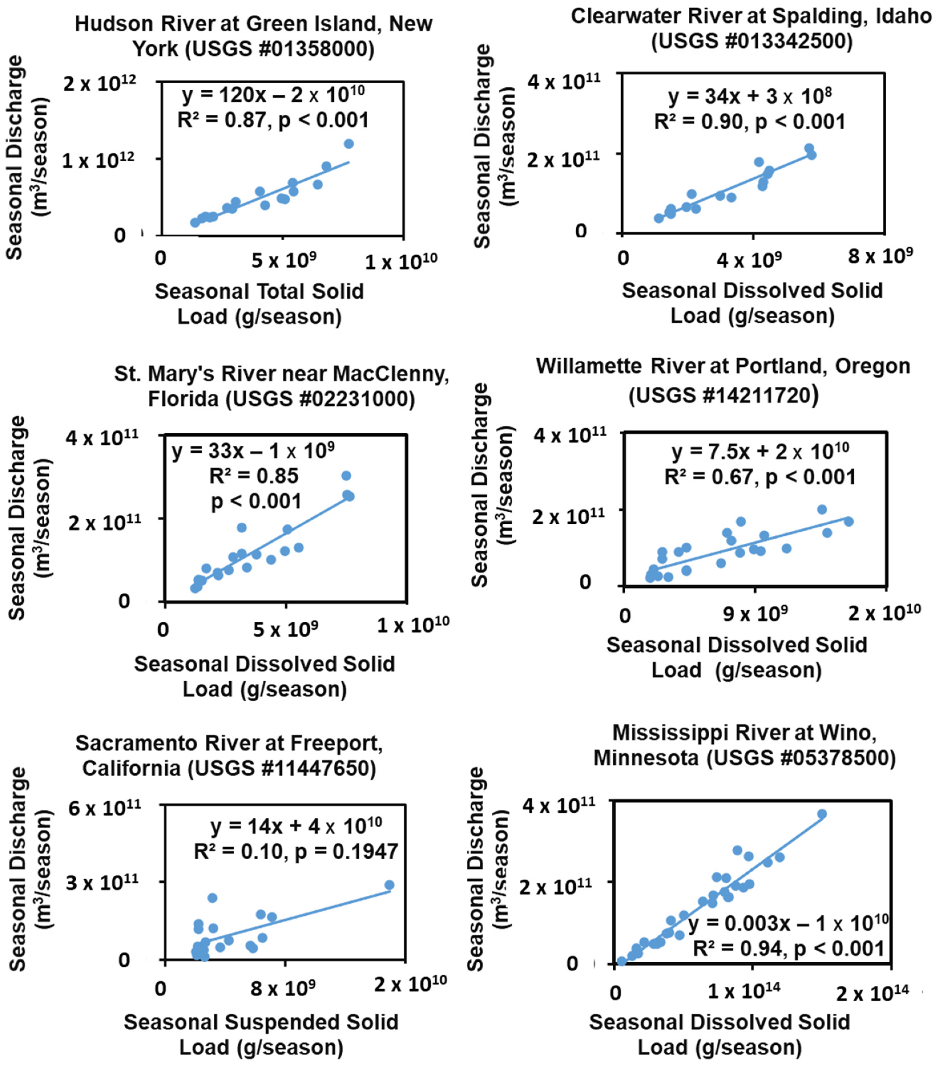
A good linear correlation between the measured seasonal discharge and the measured seasonal sediment load is a prerequisite to apply the flow-weighted method. Such correlation was evaluated using R2 and p-value. As shown in Figure 2, the values of R2 were 0.87 for Station #01358000, 0.85 for Station #02231000, 0.10 for Station # 11447650, 0.90 for Station # 013342500, 0.67 for Station # 14211720, and 0.94 for Station # 05378500; whereas the values of p were < 0.001 for all stations except for Station #11447650. The linear regression equation for each station was also given in Figure 2. Based on R2 and p values, good to very good linear correlations existed between the measured seasonal discharge and the measured seasonal sediment load for all the stations except for Station #11447650 (R2 = 0.10, p = 0.1947) in Sacramento River at Freeport, California. It should be noted that sediment concentration for Station #01358000 in Hudson River at Green Island, New York was measured as total solid, sediment concentration for Station #11447650 in Sacramento River at Freeport, California was measured as suspended solid, and sediment concentration for the rest of the stations was measured as dissolved solid.

3.2. Method Prediction vs. Field Measurement

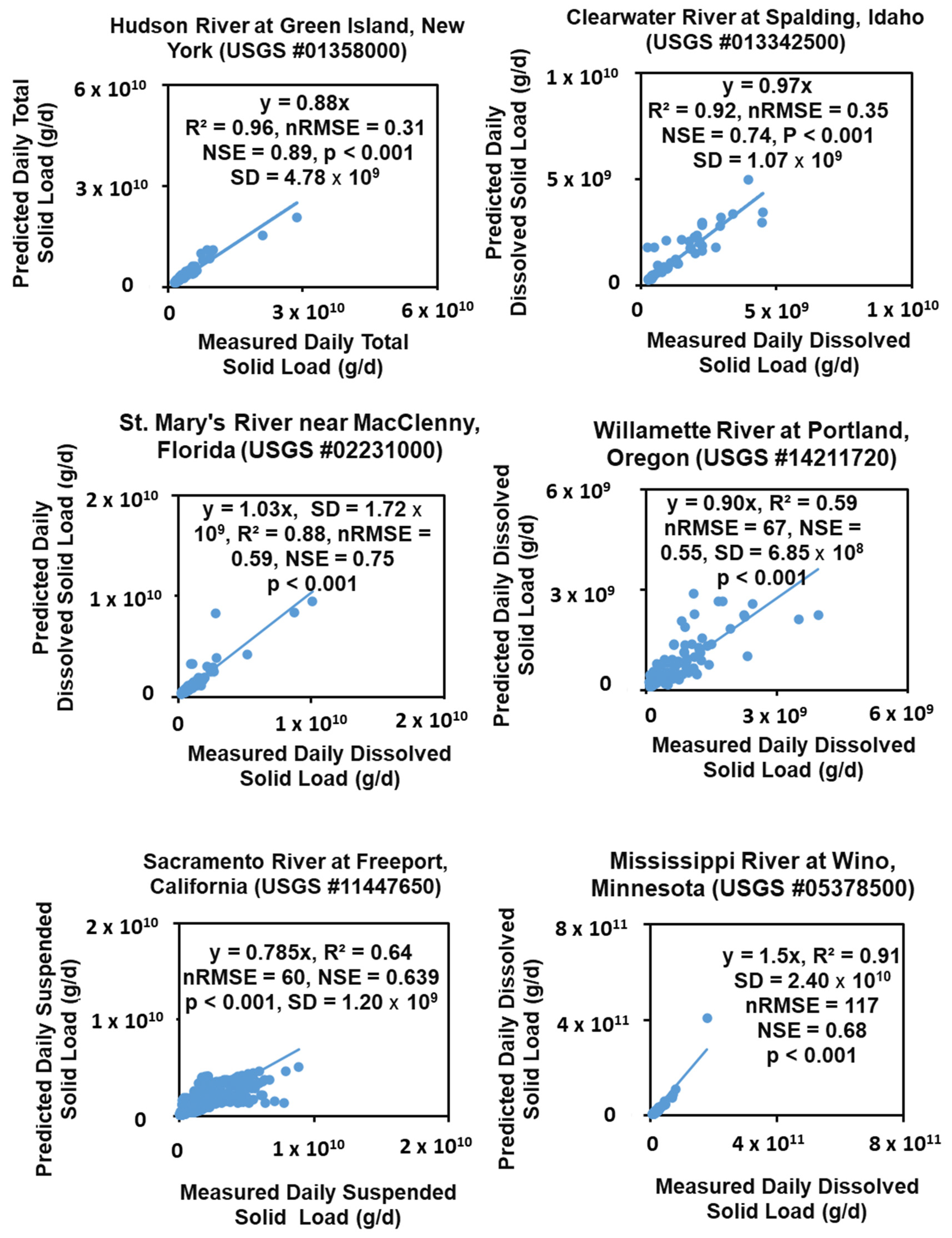
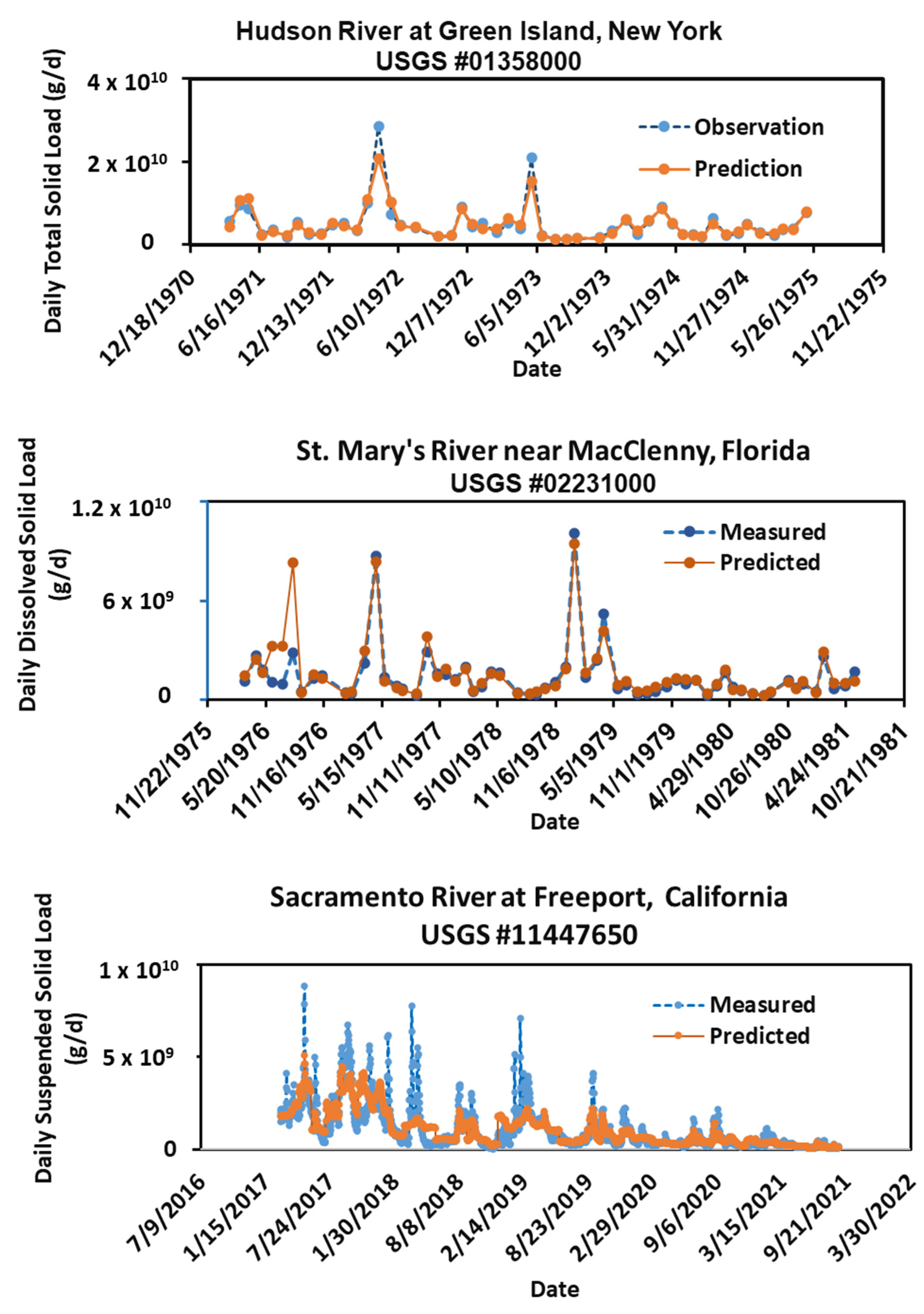
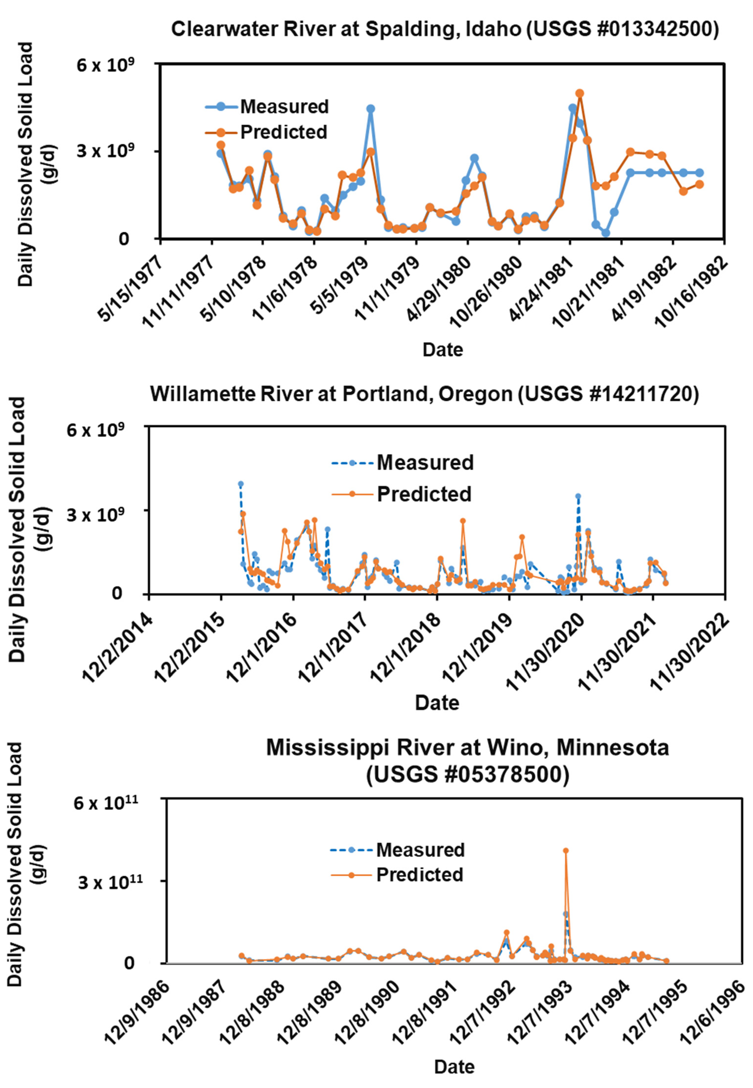
A comparison of daily sediment loads between the method predictions and the field measurements for all stations is given in Figure 3. The statistical values ranged from 0.59 to 0.96 for R2, from 0.31 to 117 g/d for nRMSE, from 0.59 to 0.89 for NSE, 6.85 × 10⁸ to 2.40 × 10¹⁰ for SD of observed data, and less than 0.001 for p-value. These statistics demonstrated that the flow-weighted method predicted the daily total sediment loads from fairly to very good, depending on the USGS stations. The graphical visualization of the peaks and valleys of daily sediment loads between the method predictions and the field measurements for all six USGS stations is shown in Figure 4 and Figure 5. In general, the predicted peaks and valleys of the daily sediment loads matched most of those measured ones well visually except for Station #11447650 located in Sacramento River at Freeport, California (Figure 4). In particular, the predicted peaks were much lower than the measured peaks, whereas the predicted valleys were higher than the measured valleys for Station #11447650.

3.3. Daily Sediment Load Prediction

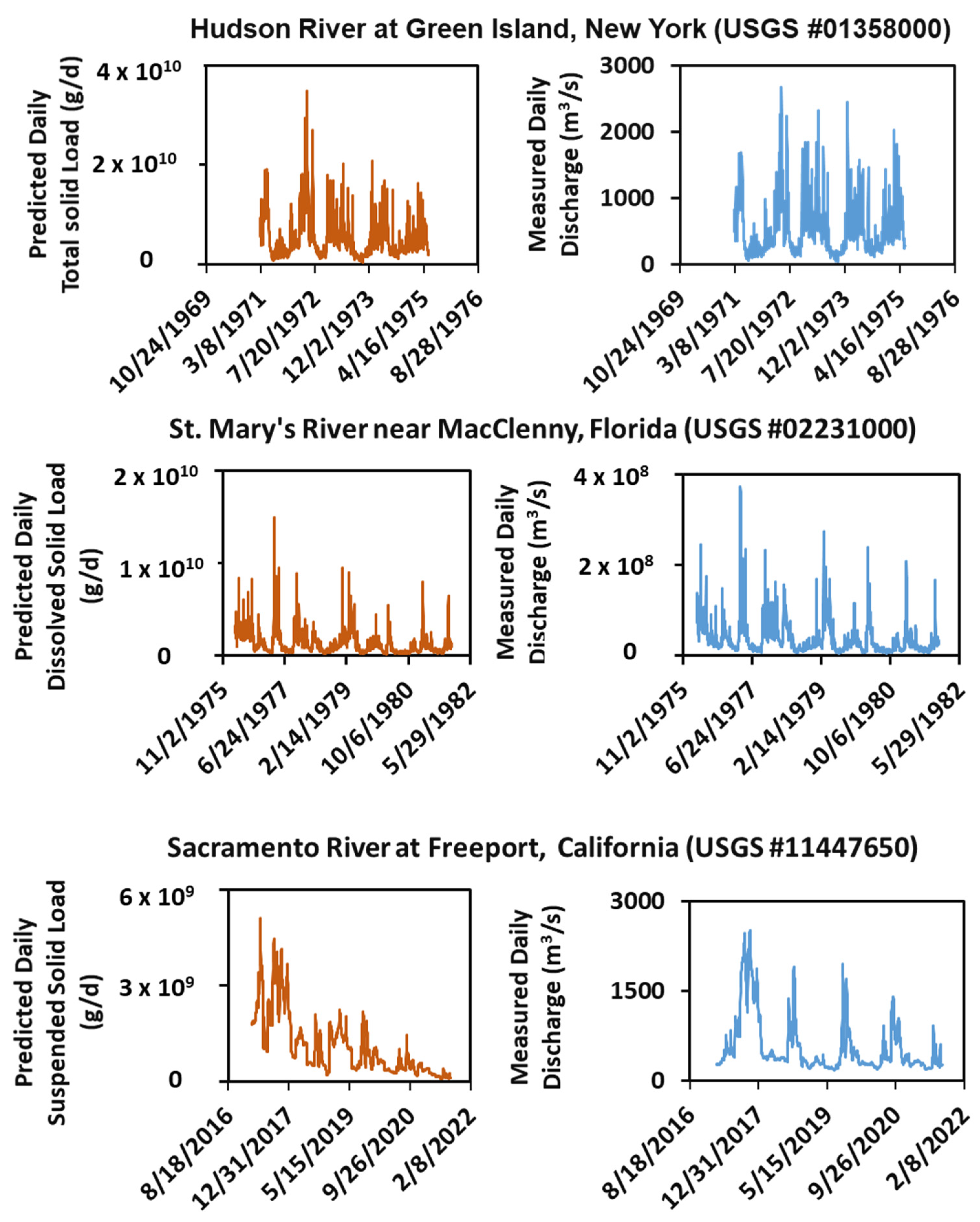
Predicted daily continuous sediment loads along with corresponding measured discharges for all six stations are shown in Figure 6 and Figure 7. The predicted peaks and valleys of the sediment loads had similar fluctuated patterns to those of the measured discharges for most stations excepted for Station #11447650 (Figure 6). That is, an increase in measured discharges increased the predicted sediment loads, whereas a decrease in the measured discharges decreased the predicted sediment loads. For example, the stream discharge increased from 810 m3/s on 1 May 1972 to 1421 m3/s on 17 May 1972 for Station #01358000 in Hudson River at Green Island, New York; whereas the predicted total solid load increased from 1.05 × 10¹⁰ to 1.85 × 10¹⁰ g/d for the same period and station. A 76% increase in discharge increased the predicted total solid load by about 75%. When the stream discharge decreased from 1421 m3/s on 17 May 1972 to 331 m3/s on 31 May 1972 at the same station, the predicted total solid load decreased from 1.85 × 10¹⁰ to 4.31 × 10⁹ g/d. A 54% decrease in discharge decreased the predicted total solid load by 42%.
For Station #11447650 in Sacramento River at Freeport, California, the fluctuated pattern of the measured discharges did not correspond well with those of the predicted daily sediment loads (Figure 6). In other words, an increase in the measured daily discharges may not increase the predicted daily sediment loads. For instance, there was a highest peak of the predicted sediment load (5.1 × 10⁹ g/d) on 11 May 2017, but there was no peak of the measured discharge at the same date (Figure 6).

4. Discussion

A major assumption in applying the flow-weighted method to predict the daily continuous sediment loads is that a good linear correlation exists between the measured seasonal discharges and the measured seasonal sediment loads. This correlation was tested using the R2 and p value. It should be noted that a good linear correlation determined by R2 varies with research discipline and there is no standard guideline to decide which value is acceptable. Henseler et al. [25] proposed a rule of thumb for acceptable R2 with 0.75 as substantial, 0.50 as moderate, and 0.25 as weak. Since watershed stream discharge and sediment load are highly dynamic and complex processes, a good linear correlation is determined when R2 ≥ 0.75 and p < 0.01. Based on this criterion, the flow-weighted method can be used to predict daily continuous sediment loads for all stations except for Station #11447650 (R2 = 0.10, p = 0.20). In other words, five USGS stations, namely Stations #01358000, #02231000, # 013342500, # 14211720 and #05378500, should be retained for predicting daily sediment loads using the flow-weighted method.
An elaborate observation of the measured sediment data listed in Table 1 revealed that although there was one measured sediment data point in most of the months within a season, there were some missing measured data in certain months within a season for each USGS station. For example, the measured sediment data were missing in August 1972 for Station #01358000, December 1976 for Station #02231000, and February 1980 for Station #013342500. These occasional missing monthly data seem to be acceptable as the good linear correlations between the measured seasonal discharges and the measured seasonal sediment loads still existed in the datasets for the three stations (Figure 2). Ideally, it would be better if there was one measured sediment data each month within a season in applying the flow-weighted method.
To develop confidence in applying the flow-weighted method, a comparison of daily sediment loads between method predictions and field measurements is necessary. Based on the statistical analyses (R2, nRMSE, NSE, SD, and p-value) shown in Figure 3, the flow-weighted method well predicted the daily sediment loads for the five USGS stations that had good linear correlations between the measured seasonal discharges and the measured seasonal sediment loads. It should be pointed out that the values of the nRMSE shown in Figure 3 varied from 0.31 to 117 g/d. Ideally, the best value of nRMSE or RMSE (root mean square error) for an optimal comparison between the method predictions and field measurements would be zero. In practice, the value of the zero nRMSE or RMSE is seldom achieved. Kastridis et al. [26] reported an acceptable RMSE is that the value of RMSE/SD is < 0.65 and SD is from observed data. In this study, the values of RMSE/SD and PBIAS (percent bias) are, respectively, 0.33 and −2.5 for Station #01358000, 0.15 and −1.5 for Station #02231000, 0.60 and −2.7 for Station #11447650, 0.36 and 3.6 for Station #013342500, 0.67 and 6.9 for Station #14211720, and 1.18 and 17.2 for Station #05378500. Although the value (1.18) of RMSE/SD for Station #05378500 is > 0.65, the other statistical measures such as R2, NSE, PBIAS, and p-value for this station are acceptable. Additionally, very good agreements of the peaks and valleys between the measured and predicted daily sediment loads for the five stations (Figure 4 and Figure 5) further confirmed that the flow-weighted method is a useful tool to predict daily sediment loads when the sparse measured data are available.
Very few studies are performed to predict sediment loads based on sparse, discontinuous, and intermittent measured data. Park et al. [27] identified the correlation between the sparse measured data and the LOADEST model predictions in annual sediment loads for five USGS stations across the US. These authors found that using the mean flow calibrated by the regression equations of LOADEST reduces errors in annual sediment load from −39.7 to −10.8% as compared to using the measured data. Apparently, the LOADEST model is not an ideal tool to predict annual sediment loads in their study. As shown in Figure 3, the flow-weighted method used in this study not only predicted daily sediment loads but also matched the peaks and valleys of the daily sediment loads well.
For a demonstration purpose on how the flow-weighted method predicts daily sediment loads when a poor linear correlation presents between the measured seasonal discharges and the measured seasonal sediment loads, Station #11447650 (R2 = 0.10, p = 0.20) was included in the validation study. Results indicated that the flow-weighted method did not predict the daily sediment loads well, especially the peaks and valleys (Figure 6), for this station. Therefore, it is not advised to use the flow-weighted method when a poor correlation presented. Although the reasons for a poor correlation between the measured seasonal discharges and the measured seasonal sediment loads for this station remain to be investigated, a possible explanation would be the sediment concentration at this station was measured as suspended solid. Suspended solids may deposit to the stream bed when the stream discharges are at a low flow velocity. In other words, a poor linear correlation may exist between suspended solid concentrations and stream discharge at a low flow velocity [28].
The predicted daily sediment loads had a similar fluctuation pattern as that of the measured daily stream discharges. This is expected because a good linear correlation between the seasonal sediment loads and the seasonal discharges exists, which is a prerequisite in applying the flow-weighted method. When this prerequisite did not meet, different fluctuating patterns in peaks and valleys between the predicted daily sediment loads and the measured daily stream discharges occurred as shown in Figure 6 for Station #11447650 in Sacramento River at Freeport, California. Under this condition, the flow-weighted method may not be applicable to predict daily sediment load.

5. Summary

Sediment contamination and deposition in rivers and streams are serious environmental and ecological concerns. While the sparse, intermittent, and discontinuous measured daily sediment data may exist for some watersheds, the long-term and continuous measured daily sediment data in most watersheds around the world are not available because of time-consuming and budget constraint. However, when developing TMDL and performing model calibration and validation for sediments, such a long-term and continuous daily dataset is essential.
The flow-weighted method, developed by Ouyang [20], was employed to predict daily sediment loads using the sparse, intermittent, and discontinuous measured data. The method predictions were validated with measured data from six different USGS gage stations across the US, indicating that the flow-weighted method is capable to fill the daily sediment load data gaps.
A good linear correlation between measured seasonal discharge and measured seasonal sediment load is a prerequisite in applying the flow-weighted method. Ideally, it would be better if there is one measured daily sediment data each month within a season in applying the flow-weighted method although some missing daily data for certain months seem to be acceptable provided a good linear correlation between the measured seasonal discharges and measured seasonal sediment loads exists.

Supplementary Materials

The following are available online at https://www.mdpi.com/article/10.3390/hydrology9100181/s1, Table S1: Stream discharge data from Station #01358000, Table S2: Sparse measured sediment data from Station #01358000, Figure S1: R script used to implement the flow-weighted method for Station #01358000. Tables S1 and S2 are the input data files for the R script.

Funding

This research received no external funding.

Data Availability Statement

All data are available in the manuscript and the Supplementary Materials Section.

Conflicts of Interest

The author declares no conflict of interest.

References

  1. Ouyang, Y.; Higman, J.; Campbell, D.; Davis, J. Three-dimensional kriging analysis of sediment mercury distribution: A case study. J. Am. Water Resour. Assoc. 2003, 39, 689–702. [Google Scholar] [CrossRef]
  2. Simon, A.; Darby, S.E. Effectiveness of grade-control structures in reducing erosion along incised river channels: The case of Hotophia Creek, Mississippi. Geomorphology 2002, 42, 229–254. [Google Scholar] [CrossRef]
  3. Almasalmeh, O.; Saleh, A.A.; Mourad, K.A. Soil erosion and sediment transport modelling using hydrological models and remote sensing techniques in Wadi Billi, Egypt. Model. Earth Syst. Environ. 2022, 8, 1215–1226. [Google Scholar] [CrossRef]
  4. Noe, G.B.; Cashman, M.J.; Skalak, K.; Gellis, A.; Hopkins, K.G.; Moyer, D.; Webber, J.; Benthem, A.; Maloney, K.; Brakebill, J.; et al. Sediment dynamics and implications for management: State of the science from long-term research in the Chesapeake Bay watershed, USA. Wires Water 2020, 7, 1454. [Google Scholar] [CrossRef]
  5. Ouyang, Y.; Leininger, T.D.; Moran, M. Impacts of reforestation upon sediment load and water outflow in the Lower Yazoo River Watershed, Mississippi. Ecol. Eng. 2013, 61, 394–406. [Google Scholar] [CrossRef]
  6. Ferreira, C.S.S.; Seifollahi-Aghmiuni, S.; Destouni, G.; Ghajarnia, N.; Kalantari, Z. Soil degradation in the European Mediterranean region: Processes, status and consequences. Sci. Total Environ. 2022, 805, 150106. [Google Scholar] [CrossRef]
  7. Kastridis, A.; Stathis, D.; Sapountzis, M.; Theodosiou, G. Insect Outbreak and Long-Term Post-Fire Effects on Soil Erosion in Mediterranean Suburban Forest. Land 2022, 11, 911. [Google Scholar] [CrossRef]
  8. Adnan, R.M.; Liang, Z.M.; El-Shafie, A.; Zounemat-Kermani, M.; Kisi, O. Prediction of Suspended Sediment Load Using Data-Driven Models. Water 2019, 11, 2060. [Google Scholar] [CrossRef] [Green Version]
  9. Banadkooki, F.B.; Ehteram, M.; Ahmed, A.N.; Teo, F.Y.; Ebrahimi, M.; Fai, C.M.; Huang, Y.F.; El-Shafie, A. Suspended sediment load prediction using artificial neural network and ant lion optimization algorithm. Environ. Sci. Pollut. Res. 2020, 27, 38094–38116. [Google Scholar] [CrossRef]
  10. Chiang, L.C.; Liao, C.J.; Lu, C.M.; Wang, Y.C. Applicability of modified SWAT model (SWAT-Twn) on simulation of watershed sediment yields under different land use/cover scenarios in Taiwan. Environ. Monit. Assess. 2021, 193, 520. [Google Scholar] [CrossRef]
  11. Van Campenhout, J.; Petit, F.; Peeters, A.; Houbrechts, G. Estimation of the area-specific suspended sediment yield from discrete samples in different regions of Belgium. J. Soil Sediment 2022, 22, 704–729. [Google Scholar] [CrossRef]
  12. Arnold, J.G.; Moriasi, D.N.; Gassman, P.W.; Abbaspour, K.C.; White, M.J.; Srinivasan, R.; Santhi, C.; Harmel, R.D.; van Griensven, A.; Van Liew, M.W.; et al. SWAT: Model Use, Calibration, and Validation. Trans. ASABE 2012, 55, 1491–1508. [Google Scholar] [CrossRef]
  13. Bicknell, B.R.; Imhoff, J.C.; Kittle, J.L., Jr.; Jobes, T.H.; Donigian, A.S., Jr.; Johanson, R. Hydrological Simulation Program-Fortran: HSPF Version 12 User’s Manual; AQUA TERRA Consultants: Mountain View, CA, USA, 2001; p. 845. [Google Scholar]
  14. Bingner, R.; Theurer, F. AnnAGNPS Technical Processes (Version 2); National Sedimentation Laboratory: Oxford, MS, USA, 2001.
  15. Schwarz, G.E.; Hoos, A.B.; Alexander, R.; Smith, R. The SPARROW Surface Water-Quality Model: Theory, Application and User Documentation; US Geological Survey: Drive Reston, VA, USA, 2006.
  16. Williams, J.R.; Harman, W.L.; Magre, M.; Kizil, U.; Lindley, J.A.; Padmanabhan, G.; Wang, E. Apex feedlot water quality simulation. Trans. ASABE 2006, 49, 61–73. [Google Scholar] [CrossRef]
  17. USEPA. Clean Water Act Section 303(d): Impaired Waters and Total Maximum Daily Loads (TMDLs). Available online: https://www.epa.gov/tmdl (accessed on 11 October 2022).
  18. Runkel, R.L.; Crawford, C.G.; Cohn, T.A. 2004 Load Estimator(LOADEST)—A FORTRAN Program for Estimating Constituent Loads in Streams and Rivers. In US Geological Survey Techniques and Methods; Book 4; Chapter A5; 75p. Available online: http://pubs.er.usgs.gov/publication/tm4A5 (accessed on 11 October 2022).
  19. Park, Y.S.; Engel, B.A.; Frankenberger, J.; Hwang, H. A Web-Based Tool to Estimate Pollutant Loading Using LOADEST. Water 2015, 7, 4858–4868. [Google Scholar] [CrossRef] [Green Version]
  20. Hirsch, R.M. Large Biases in Regression-Based Constituent Flux Estimates: Causes and Diagnostic Tools. J. Am. Water Resour. Assoc. 2014, 50, 1401–1424. [Google Scholar] [CrossRef]
  21. Ouyang, Y. A flow-weighted approach to generate daily total phosphorus loads in streams based on seasonal loads. Environ. Monit. Assess. 2021, 193, 422. [Google Scholar] [CrossRef]
  22. Taebi, A.; Mansy, H.A. Time-frequency distribution of seismocardiographic signals: A comparative study. Bioengineering 2017, 4, 32. [Google Scholar] [CrossRef]
  23. Nash, J.E.; Sutcliffe, J.V. River flow forecasting through conceptual models part I—A discussion of principles. J. Hydrol. 1970, 10, 282–290. [Google Scholar] [CrossRef]
  24. Krause, T.; Beck, E.V.; Cherkaoui, R.; Germond, A.; Andersson, G.; Ernst, D. A comparison of Nash equilibria analysis and agent-based modelling for power markets. Int. J. Elec. Power 2006, 28, 599–607. [Google Scholar] [CrossRef] [Green Version]
  25. Henseler, J.; Ringle, C.M.; Sinkovics, R.R. New Challenges to International Marketing; Emerald Group Publishing Limited: Bingley, UK, 2009. [Google Scholar]
  26. Kastridis, A.; Theodosiou, G.; Fotiadis, G. Investigation of Flood Management and Mitigation Measures in Ungauged NATURA Protected Watersheds. Hydrology 2021, 8, 170. [Google Scholar] [CrossRef]
  27. Park, Y.S.; Engel, B.A. Identifying the Correlation between Water Quality Data and LOADEST Model Behavior in Annual Sediment Load Estimations. Water 2016, 8, 368. [Google Scholar] [CrossRef]
  28. Ellison, C.A.; Kiesling, R.L.; Fallon, J.D. Correlating streamflow, turbidity, and suspended-sediment concentration in Minnesota’s Wild Rice River. In Proceedings of the 2nd Joint Federal Interagency Conference, Las Vegas, NV, USA, 27 June–1 July 2010. [Google Scholar]
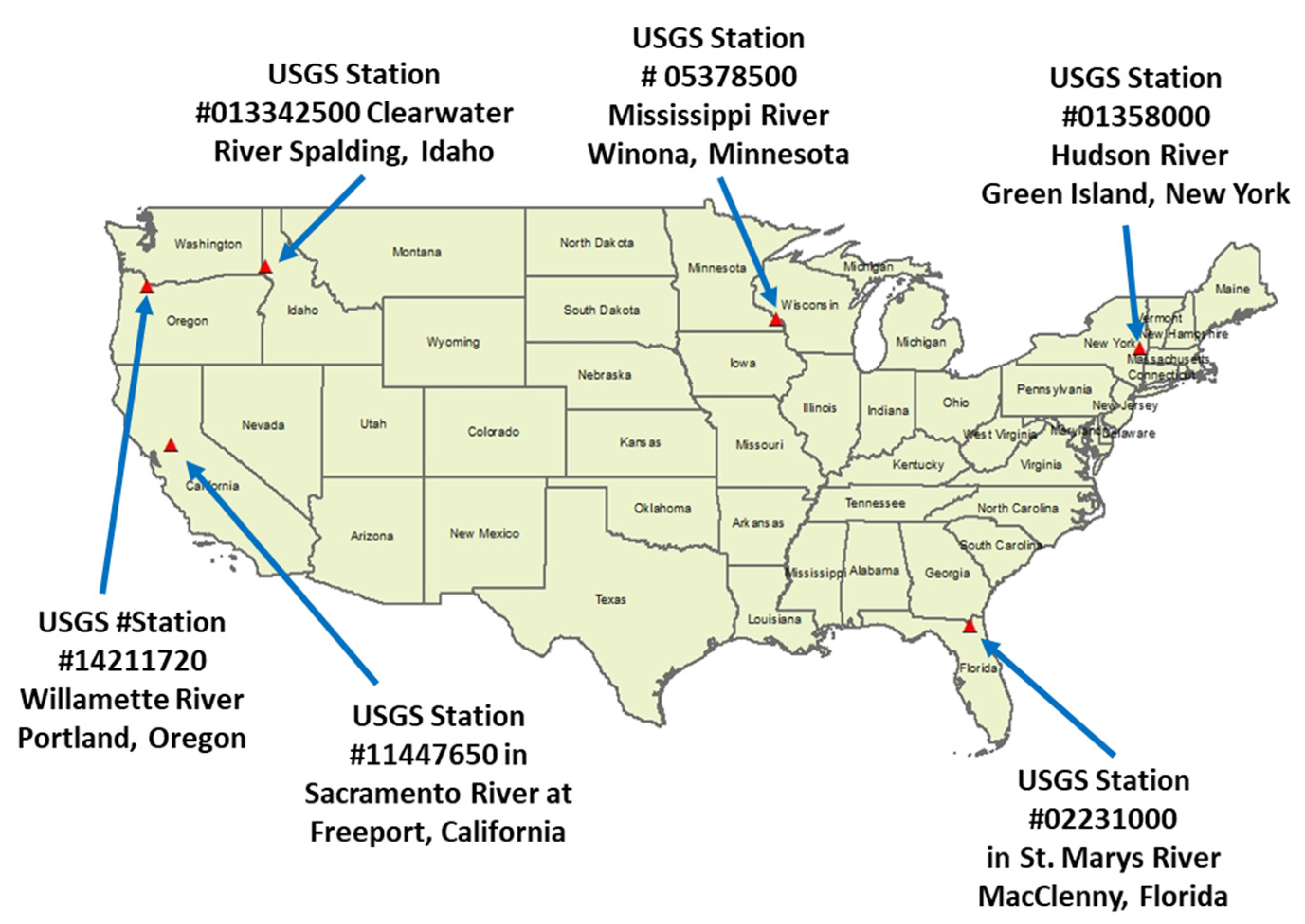
Figure 1. Locations of US Geological Survey gage stations used in this study.
Hydrology 09 00181 g001
Figure 2. Correlations between the measured seasonal sediment loads and the measured seasonal discharges for the six USGS gage stations.
Hydrology 09 00181 g002
Figure 3. Comparisons of the daily sediment loads between the method predictions and the field measurements for the six USGS stations.
Hydrology 09 00181 g003
Figure 4. Comparisons of the daily sediment loads between the method predictions and the field measurements for Stations #013580003500, #02231000, and #11447650.
Hydrology 09 00181 g004
Figure 5. Comparisons of the daily sediment loads between the method predictions and the field measurements for Stations #013342500, #14211720, and #05378500.
Hydrology 09 00181 g005
Figure 6. Predicted daily sediment loads and their corresponding measured daily discharges for Stations #013580003500, #02231000, and #11447650.
Hydrology 09 00181 g006
Figure 7. Predicted daily sediment loads and their corresponding measured daily discharges at Stations #013342500, #14211720, and #05378500.
Hydrology 09 00181 g007
Table 1. Sparse measured daily sediment data at Stations #013580000, #02231000, and #013342500.
USGS #01358000USGS #02231000USGS #013342500
Hudson River at Green Island, New YorkSt. Marys River near MacClenny, FloridaClearwater River at Spalding, Idaho
DateTotal Solid (mg/L)DateDissolved Solid (mg/L)DateDissolved Solid (mg/L)
3/29/19711733/16/19762712/14/197747
4/26/19711164/19/1976381/26/197840
5/17/19711025/11/1976382/16/197842
6/22/19711516/9/1976253/22/197839
7/20/19711507/12/1976234/19/197830
8/25/19711038/11/1976265/25/197833
9/23/19711559/7/1976316/19/197826
10/21/197111710/14/1976267/20/197825
11/23/197114111/11/1976348/23/197832
12/21/19711281/24/1977339/21/197832
1/19/19721682/9/19772410/19/197843
2/23/19721313/23/19773011/15/197835
3/22/19721364/26/19774212/13/197835
4/19/19722075/24/1977491/18/197938
5/23/19721096/30/1977442/14/197967
6/15/19721457/19/1977453/21/197944
7/25/19721348/31/1977264/18/197943
9/21/197211410/3/1977295/22/197925
10/26/197211711/2/1977426/27/197921
11/21/197212611/29/1977327/25/197932
12/19/19729212/29/1977278/22/197929
1/16/19731461/30/1978269/12/197929
2/20/1973802/22/19782110/24/197933
3/23/1973853/21/19781911/19/197940
4/24/1973804/18/19782512/18/197933
5/22/19731375/16/1978271/23/198034
6/18/19731277/11/1978383/17/198053
7/24/19731048/16/1978284/22/198026
8/22/19731169/8/1978305/21/198022
9/18/197310910/4/1978526/18/198026
11/14/197313411/3/1978617/21/198027
12/18/197312512/5/1978618/14/198027
1/24/1974951/3/1979609/23/198034
2/20/1974752/6/19794810/23/198036
3/22/19741203/14/19793211/18/198027
4/25/19741294/3/19794112/18/198029
5/24/19741215/15/1979261/23/198134
6/20/19741196/13/1979313/17/198134
7/17/19741317/17/1979235/2/198127
8/8/19741088/14/1979255/26/198144
9/5/19741659/11/1979246/23/198130
10/11/197411610/16/1979277/23/198130
11/11/197411511/14/1979368/26/198130
12/3/197410112/12/1979309/24/198135
1/7/19751001/16/19803711/19/198149
2/11/1975792/20/1980291/27/198248
3/7/1975843/18/1980203/11/198247
4/2/19751034/15/1980215/25/198227
5/6/1975885/7/1980287/21/198231
6/4/1980259/24/198233
7/8/19802611/18/198236
8/11/198030
9/3/198030
10/28/198041
11/19/198040
12/9/198032
1/20/198141
2/12/198135
3/17/198126
4/21/198132
5/21/198157
Table 2. Some measured seasonal sediment load calculations for Station #01358000.
ABCDEF
Date Total Solid (mg/L) Average Seasonal Total Solid Concentration (mg/L) Season Streamflow Volume (m3/Season)Season Total Solid Load (g/Season)Season
3/29/1971 173
4/26/1971 116
5/17/1971 102 130.33 6.94 × 1099.05 × 1011spring
6/22/1971 151
7/20/1971 150
8/25/1971 103 134.67 1.69 × 1092.27 × 1011summer
9/23/1971 155
10/21/1971 117
11/23/1971 141 137.67 1.81× 1092.49 × 1011fall
12/21/1971 128
1/19/1972 168
2/23/1972 131 142.33 3.08 × 1094.39 × 1011winter
3/22/1972 136
4/19/1972 207
5/23/1972 109 150.67 7.90 × 1091.19 × 1011spring
6/15/1972 145
7/25/1972 134 139.50 4.15 × 1095.78 × 1011summer
9/21/1972 114
10/26/1972 117
11/21/1972 126 119.00 2.94 × 1093.49 × 1011fall
12/19/1972 92
1/16/1973 146
2/20/1973 80 106.00 winter
3/7/1975 84
4/2/1975 103
5/6/1975 88 91.67 5.19 × 1094.76 × 1011Spring
Table 3. Calculated partitioning coefficients and predicted daily total solid loads for Station #01358000.
ABCDEFGH
DateMeasured Daily Discharge (m3/s)Measured Daily Discharge (m3/day)Measured Seasonal Discharge Volume (m3/season)Measured Seasonal Total Solid Load (g/season)Daily Flow-Weighted Partitioning CoefficientPredicted Daily Total Solid Load (g/day)Season
3/1/1971832.527.19 × 1076.94 × 1099.05 × 10110.010369.37 × 109Spring
3/2/1971809.867.00 × 107 0.010089.12 × 109
3/3/1971733.416.34 × 107 0.009138.26 × 109
3/4/1971637.135.50 × 107 0.007937.17 × 109
3/5/1971543.684.70 × 107 0.006776.12 × 109
5/28/1971538.024.65 × 107 0.006706.06 × 109
5/29/1971399.273.45 × 107 0.004974.50 × 109
5/30/1971396.443.43 × 107 0.004934.46 × 109
5/31/1971353.963.06 × 107 0.004413.99 × 109
6/1/1971351.133.03 × 1071.69 × 1092.27 × 10110.017974.09 × 109Summer
6/2/1971300.162.59 × 107 0.015363.49 × 109
6/3/1971286.002.47 × 107 0.014643.33 × 109
6/4/1971294.502.54 × 107 0.015073.43 × 109
6/5/1971243.812.11 × 107 0.012482.84 × 109
6/6/1971239.282.07 × 107 0.012252.78 × 109
6/7/1971223.421.93 × 107 0.011432.60 × 109
Publisher’s Note: MDPI stays neutral with regard to jurisdictional claims in published maps and institutional affiliations.