A Practical Unified Algorithm of P-IMC Type

Abstract

The paper presents a practical algorithm of the proportional-internal model control (P-IMC) type that can be applied to control a wide class of processes: Stable proportional processes, integral processes and some unstable processes. The P-IMC algorithm is a suitable combination between the P0-IMC algorithm and the P1-IMC algorithm, which are characterized by a too weak and a too strong impact of the tuning gain on the control action, respectively. The overall controller has five parameters: A tuning parameter K, three model parameters (steady-state gain, settling time, and time delay) and a process feedback gain used only for integral or unstable processes, to turn them into a compensated process (stable and of proportional type). For a step setpoint, the initial value of the compensated process input is approximately K times its final value. Furthermore, for $K=1$, the compensated process input is close to a step shape (step control principle). These properties enable a human operator to check and adjust online the model parameters. Due to its control performance, robustness to modeling error, and capability to be easily tuned and applied for all industrial processes, the P-IMC algorithm could be a viable alternative to the known PID algorithm. Numerical simulations are given to highlight the performance and the flexibility of the algorithm.

1. Introduction

In spite of all recent advances in control technology, the old proportional-integral-derivative (PID) algorithm is still by far the most widely used in practice due to its simplicity, feasibility, and capacity to control almost all plant types [1,2,3]. However, for many complex processes, especially with overshoot, time delay, non-minimum phase, and/or non-linear characteristics, the PID algorithm cannot achieve good and very good control performances. Also, there is not a simple unified procedure for tuning controller parameters [4,5,6,7,8].

According to the IMC principle, an accurate control can be achieved if a suitable model of the process is encapsulated in the control system structure [9,10,11,12,13]. Despite their many advantages, the algorithms of the IMC-type have not become a convincing practical alternative to PID algorithm [14,15,16] because there is no simple model structure for all types of process. Over the past 10–20 years, many PID tuning methods have been developed by applying IMC techniques for processes of low order plus time delay [17,18,19]. However, the control performance derived by implementing IMC-based PID algorithms is usually weaker than that obtained by using genuine IMC algorithms (especially for processes with large time delay).

We have presented in 2017 and 2018 two unified control algorithms [20,21] of P0-IMC type and P1-IMC type, respectively, whose bloc-diagrams are illustrated in Figure 1 and Figure 2, where $G_P\left(s\right)$ is the process transfer function, $G_M\left(s\right)$ is the transfer function of the compensated process model, $K_M$ is the model steady-state gain, $K_f$ is the process feedback gain, K is the tuning gain, Y is the controlled variable, R is the setpoint (reference), E is the error (offset), U is the control variable, V is the disturbance, and C is the internal control variable.

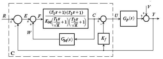
Figure 1. Closed-loop system with proportional-internal model control (P-IMC) controller, P0-IMC type.

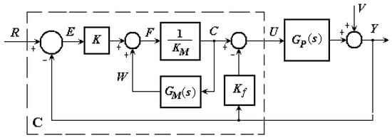
Figure 2. Closed-loop system with P1-IMC controller.

The direct feedback path of the process, characterized by the gain $K_f$, is used only for integral and some unstable processes, in order to convert the original process P into a stable proportional process P0 (with the gain $K_{P_0}$ bounded and nonzero), called compensated process. The process compensation technique has been firstly used in [22,23] for unstable processes, and in [24] for stable integral processes. For stable proportional processes, the feedback gain $K_f$ is fixed to zero, so that the compensated process and the original process are one and the same, and the control variables C and U are identical. The compensated process models in Figure 1 and Figure 2 have, respectively, the transfer functions

$$G_M\left(s\right)=\frac{K_M{e}^{-{\tau }_{M}s}}{(T_{1}s+1)(T_{2}s+1)},T_2=2T_1,$$

(1)

and

$$G_M\left(s\right)=\frac{K_M{e}^{-{\tau }_{M}s}}{{(T_{1}s+1)}^2}.$$

(2)

The algorithms P0-IMC and P1-IMC have five parameters: A tuning parameter K (with standard value 1), a process feedback gain $K_f$ (with standard value 0), and three model parameters (steady-state gain $K_M$, settling time $T_{sM}$, and time delay ${\tau }_M$). The lag time constants $T_1$ in models (1) and (2) are, respectively, given by

$$T_1=\frac{T_{s95}-{\tau }_M}{7.36}\mathrm{and}{T}_1=\frac{T_{s95}-{\tau }_M}{4.74},$$

(3)

where $T_{s95}$ is the model settling time.

For both closed-loop control systems, the steady-state error to a step reference or disturbance is zero. In addition, if the process is of integral type, the steady-state error to a ramp disturbance is zero.

Because of the initial sluggishness of the process and process model, the initial value of the control system response $c\left(t\right)$ to a unit step setpoint is for both control algorithms

$$c\left(0_{+}\right)=\frac{K}{K_M}.$$

(4)

On the other hand, since the steady-state error to a step setpoint is zero, the final value of the control system response $c\left(t\right)$ is the reverse of the steady-state gain of the compensated plant:

$$c(\infty )=\frac{1}{K_{P_0}}.$$

(5)

Therefore, for a compensated process model with $K_M=K_{P_0}$, the initial value of $c\left(t\right)$ is K times its final value:

$$c\left(0_{+}\right)=Kc(\infty ).$$

(6)

Since the model of the compensated plant is stable and of proportional type, both algorithms are unified and quasi-universal, in the sense that they have a unique form (as the PID algorithm) and may be used to control almost all industrial plants: Stable plants of proportional type (with or without overshoot, time delay and oscillations, of minimum or non-minimum phase), integral plants, and unstable plants.

The model parameters can be experimentally identified using the compensated plant response to a step input, and can be easily adjusted online. Also, by setting a suitable tuning gain K, the closed-loop control system can have good performance even if the model parameters are not accurately known.

The proposed control algorithm is of P-IMC type, and provides an adequate trade-off between the algorithms P0-IMC and P1-IMC, ensuring a moderate impact of the tuning gain K on the control action. In most practical applications, it is not desirable to use large values of the gain K (larger than 10) to avoid an excessive noise amplification and a very sharp-shrill form of the controller output $c\left(t\right)$ to a step setpoint or disturbance. The P0-IMC algorithm can lead to such undesirable situations when the parameters of the compensated plant are inaccurately selected ($K_M>>K_{P_0}$ or ${\tau }_M>>{\tau }_{P_0}$ or $T_s>>T_{s{P}_0}$) and the tuning gain K has a weak influence on the control action [20]. On the contrary, such situations are not possible by using the P1-IMC algorithm, characterized by a strong influence of K on the control action [21]. By using the new proposed algorithm, the best control performance is usually obtained for $1<K<5$, and the response $c\left(t\right)$ to a step reference is smoother than the response of the first algorithm and sharper than the one of the second algorithm. Also, for $K=$1, the new algorithm preserves the step control principle, which states that “the control response $c\left(t\right)$ to a step setpoint is close to a step form if the dynamic model of the compensated plant has a high accuracy”. By a simple analysis of the deviation of the response $c\left(t\right)$ from the step function, the model parameters can be suitably adjusted online.

Section 2 presents the theoretical basis of the P-IMC algorithm in continuous and discrete-time, and how it can be used to control stable proportional processes, integral processes, and some unstable processes in a coherent framework. In addition, the conditions for a bumpless transfer between the MANUAL, COMPENSATORY, and AUTOMATIC modes are given in discrete-time. Section 3 presents an experimental method of identifying the model parameters for all process types. A simple procedure which enables a human operator to verify online if the model parameters have suitable values and to adjust them is given in Section 4. Section 5 presents a two-degree of freedom variant of the algorithm. Using MATLAB/SIMULINK environments, some numerical applications are given in Section 6 to show the control performance, the robustness with respect to parameter uncertainty, and how the algorithm can be implemented to control various types of process. Conclusions and future research are presented in Section 7.

2. P-IMC Algorithm Design

As mentioned in the previous section, the impact of the tuning gain K on the control action is too weak for the P0-IMC algorithm and too strong for the P1-IMC algorithm. Consequently, a fast control system response to a step setpoint or disturbance is achieved with a control signal $c\left(t\right)$ too sharp (for K large) and too smooth (for K small), respectively. We show further that the proposed algorithm satisfactorily solves this problem.

The block diagram of the ${\mathrm{P}}_{\alpha }$-IMC algorithm (or, more simple, P-IMC algorithm) is shown in Figure 3, where the transfer functions of the compensated process model and internal controller are:

$$G_M\left(s\right)=\frac{K_M{e}^{-{\tau }_{M}s}}{(T_{1}s+1)(T_{2}s+1)},$$

(7)

$$G_i(\alpha ,s)=\frac{(T_{1}s+1)(T_{2}s+1)}{K_M(T_{3}s+1)(T_{4}s+1)},$$

(8)

with

$$T_3=\frac{T_1}{K_1},T_4=\frac{T_2}{K_1},K_1=K^{\frac{1-\alpha }{2}},\alpha \in (0,1).$$

(9)

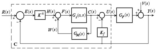
Figure 3. Proposed closed-loop system with ${\mathrm{P}}_{\alpha }$-IMC controller.

The ${\mathrm{P}}_{\alpha }$-IMC algorithm reduces to the first algorithm in Figure 1 for $\alpha =0$ and $T_2=2T_1$, and to the second algorithm in Figure 2 for $\alpha =1$ and $T_2=T_1$. By setting $K=1$, the internal controller (8) becomes purely proportional, and all three control algorithms (for $\alpha =0$, $\alpha =1$, and $0<\alpha <1$) are identical.

The following theorems are valid for a stable closed-loop control system of P-IMC type having the structure in Figure 3.

Theorem 1.

The steady-state error of an asymptotically stable control system with P-IMC controller is zero for any step setpoint or disturbance.

Proof. 

Since the compensated process is of proportional type, it suffices to prove that the transfer function $G_{CE}\left(s\right)$ between the output C and the input E is of integral type (i.e., it has a pole at the origin). This is true because

$$G_{CE}\left(s\right)=G_{HE}\left(s\right)G_{CH}\left(s\right)=K^{\alpha }·\frac{G_i(\alpha ,s)}{1-G_i(\alpha ,s)G_M\left(s\right)}$$

(10)

and

$$1-G_i(\alpha ,0)G_M\left(0\right)=1-\frac{1}{K_M}·K_M=0.$$

 ☐

Theorem 2.

The initial and final values of the control response $c\left(t\right)$ of a P-IMC controller to a unit step setpoint does not depend on the weighting coefficient α:

$$c\left(0_{+}\right)=\frac{K}{K_M},c(\infty )=\frac{1}{K_{P_0}}.$$

(11)

In addition, if $K_M=K_{P_0}$, then ${\displaystyle \frac{c\left(0_{+}\right)}{c(\infty )}}=K$.

Proof. 

Because of the initial sluggishness of the process and model, we have (see Figure 3)

$$f\left(0_{+}\right)=h\left(0_{+}\right)=K^{\alpha }e\left(0_{+}\right)=K^{\alpha }r\left(0_{+}\right)=K^{\alpha },$$

therefore

$$c\left(0_{+}\right)=G_i(\alpha ,\infty )f\left(0_{+}\right)=\frac{T_1{T}_2}{K_M{T}_3{T}_4}·K^{\alpha }=\frac{K}{K_M}.$$

On the other hand, according to Theorem 1, we have $y(\infty )=1$, therefore

$$c(\infty )=\frac{y(\infty )}{K_{P_0}}=\frac{1}{K_{P_0}}.$$

 ☐

According to Theorem 2, if $K=1$ and $K_M=K_{P_0}$, the initial and final values of the response $c\left(t\right)$ to a unit step reference are equal to each other, that is $c\left(0_{+}\right)=c(\infty )$. Moreover, the P-IMC algorithm satisfies the step control principle:

Theorem 3.

If $K=1$ and the model of the compensated process is perfect, then the control response $c\left(t\right)$ of a P-IMC controller to a unit step setpoint is a perfect step of magnitude $1/K_M$.

Proof. 

We only need to show that the transfer function $G_{CR}\left(s\right)$ is equal to $1/K_M$. According to (10), we have

$$G_{CR}\left(s\right)=\frac{G_{CE}\left(s\right)}{1+G_{CE}\left(s\right)G_{P_0}\left(s\right)}=\frac{K^{\alpha }}{G_i^{-1}(\alpha ,s)-G_M\left(s\right)+K^{\alpha }{G}_{P_0}\left(s\right)}.$$

If $K=1$ and $G_M\left(s\right)=G_{P_0}\left(s\right)$, then

$$G_{CR}\left(s\right)=G_i(\alpha ,s){\mid }_{K=1}=\frac{1}{K_M}.$$

 ☐

Assume further that the compensated process is of P*-type (proportional and having a monotone and bounded step response) and consider the model (7) with

$$T_2=\gamma T_1,\gamma \in [0,1].$$

(12)

For a given $\gamma$, the parameters of the model (7) can be experimentally determined by using the compensated plant response $y\left(t\right)$ to a step input c, as follows:

$$K_M=K_{P_0},{\tau }_M={\tau }_{P_0},$$

(13)

$$T_1=\frac{T_{tr}}{\beta \left(\gamma \right)},T_2=\gamma T_1,$$

(14)

where the computed values of the function $\beta \left(\gamma \right)$ are showed in Table 1, and $T_{tr}$ is the transient time of the response $y\left(t\right)$ (without time delay); more precisely,

$$T_{tr}=T_{s{P}_0}-{\tau }_{P_0},$$

(15)

where ${\tau }_{P_0}$ is the time delay of the compensated plant, and $T_{s{P}_0}$ the settling time of the compensated plant (when the response y reaches 95% or 98% of its final value).

Table 1. $T_1\left(\gamma \right)$ and $T_2\left(\gamma \right)$ calculation.

$\mathit{\gamma }$	$\mathit{\beta }\left(\mathit{\gamma }\right)$ for ${\mathit{T}}_{\mathit{s}95}$	$\mathit{\beta }\left(\mathit{\gamma }\right)$ for ${\mathit{T}}_{\mathit{s}98}$
0	3.00	3.91
0.1	3.10	4.02
0.2	3.22	4.14
0.3	3.35	4.27
0.4	3.50	4.42
0.5	3.68	4.60
0.6	3.87	4.80
0.7	4.07	5.03
0.8	4.28	5.28
0.9	4.51	5.55
1	4.74	5.83

For practical reasons, we will consider that the parameters of the compensated plant model are $K_M$, ${\tau }_M$, and $T_s$. As shown in [20] for $\alpha =0$ and in [21] for $\alpha =1$, if the tuning gain K is suitably selected, then an estimation of the model parameters with an error less than 15% does not significantly diminish the control performance. We claim that this robustness property is also satisfied for $0<\alpha <1$.

To get the discrete-time control algorithm, let us denote by T the sampling period and by $l_M$ the integer ratio of the model time delay to the sampling period:

$$l_M=\left[\frac{{\tau }_M}{T}\right].$$

(16)

Moreover, let us denote

$$p_1=e^{-T/T_1},p_2=e^{-T/T_2},$$

(17)

$$p_3=e^{-T/T_3},p_4=e^{-T/T_4},$$

(18)

$$q_3=1-\frac{1-p_3}{K_1},q_4=1-\frac{1-p_4}{K_1},$$

(19)

$$F=f_k-(q_3+q_4)f_{k-1}+q_3{q}_4{f}_{k-2}.$$

(20)

The discrete-time equivalent of the model (7) has the approximate transfer function

$$G_M^0\left(z\right)\approx \frac{K_M(1-p_1)(1-p_2)z^{-1-l_M}}{(1-p_1{z}^{-1})(1-p_2{z}^{-1})},$$

(21)

which leads to the difference equation

$$w_k-(p_1+p_2)w_{k-1}+p_1{p}_2{w}_{k-2}=K_M(1-p_1)(1-p_2)c_{k-1-l_M}.$$

(22)

Similarly, the discrete-time equivalent of the internal controller (8) has the approximate transfer function

$$G_i^0(\alpha ,z)\approx \frac{K_1^2(1-q_3{z}^{-1})(1-q_4{z}^{-1})}{K_M(1-p_3{z}^{-1})(1-p_4{z}^{-1})},$$

(23)

and the difference equation

$$c_k-(p_3+p_4)c_{k-1}+p_3{p}_4{c}_{k-2}=\frac{K_1^2}{K_M}·F.$$

(24)

From the controller structure in Figure 3, the difference Equation (22) of the compensated process model and the difference Equation (24) of the internal controller, we get the following discrete-time control algorithm:

$$\left\{\begin{array}{c}{e}_k=r_k-y_k\hfill \\ w_k=(p_1+p_2)w_{k-1}-p_1{p}_2{w}_{k-2}+K_M(1-p_1)(1-p_2)(c_{k-1-l_M}-u_0)\hfill \\ f_k=K^{\alpha }(e_k-e_0)+w_k\hfill \\ c_k=u_0+(p_3+p_4)(c_{k-1}-u_0)-p_3{p}_4(c_{k-2}-u_0)+{\displaystyle \frac{K_1^2}{K_M}}·F\hfill \\ u_k=c_k-K_f(y_k-y_0)\hfill \end{array},\right.$$

(25)

where $e_0$, $u_0$, and $y_0$ are, respectively, the values of e, u, and y before switching to AUTOMATIC mode.

Remark 1.

To have a bumpless transfer (without suddenly changing the process input u) for any initial error $e_0\ne 0$, the following settings must be made before switching to AUTOMATIC mode:

$$c_{k-1}=c_{k-2}=\cdots =c_{k-1-l_M}=u_0$$

(26)

and

$$w_{k-1}=w_{k-2}=0,f_{k-1}=f_{k-2}=0.$$

(27)

By replacing the equation

$$f_k=K^{\alpha }(e_k-e_0)+w_k$$

(28)

in the discrete-time algorithm (25) with

$$f_k=K^{\alpha }{e}_k+w_k,$$

(29)

a bumpless transfer is achieved only for $e_0=0$. For $e_0\ne 0$, the control variables c and u modify to diminish the error as in the case of a step reference of magnitude $e_0$.

For $K_f\ne 0$, the overall controller C in Figure 3 has three distinct operating modes: AUTOMATIC, MANUAL, and COMPENSATORY. Note that in MANUAL and COMPENSATORY modes, the human operator can directly change the original process input u and the compensated process input c, respectively. Before switching to COMPENSATORY mode, characterized by the equation

$$u_k=c-K_f(y_k-y_0),$$

(30)

$y_0$ and c need to be automatically initialized to the current values of y and u, respectively. For $K_f=0$, the MANUAL and COMPENSATORY modes coincide.

Remark 2.

For integral or unstable processes, the model addresses the compensated process. The feedback gain $K_f$ is selected to get a stable proportional compensated process.

Remark 3.

For an integral process, the compensated process response $y\left(t\right)$ to a ramp disturbance v and fixed c (see Figure 3) is bounded. As a result, since the controller with the transfer function $G_{CE}\left(s\right)$ given by (10) is of integral type (see the proof of Theorem 1), the steady-state error is zero for a ramp disturbance added to the plant output.

Remark 4.

In practical applications, due to the process nonlinearities and model inaccuracy, the closed-loop response $c\left(t\right)$ to a step setpoint is not a perfect step for $K=1$. By comparing the current response $c\left(t\right)$ with the step form, the human operator can online check the accuracy of the model parameters and suitably adjust them.

Remark 5.

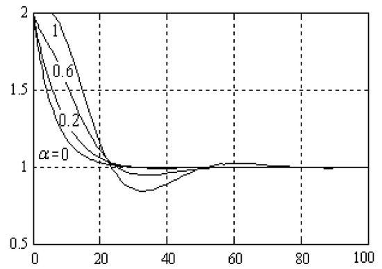
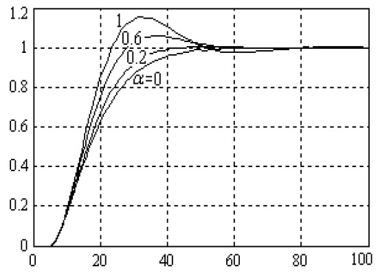
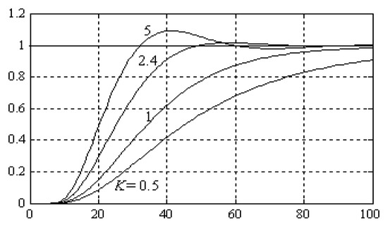
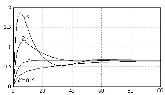
The impact of the tuning gain K on the control action is stronger for larger α. This is illustrated in Figure 4 and Figure 5 for the process

$$G_P\left(s\right)=\frac{e^{-5s}}{{(10s+1)}^2},$$

(31)

$G_M\left(s\right)=G_P\left(s\right)$, $K_f=0$, $K=2$ and four values of α. The control algorithms with $\alpha =0.2$ and $\alpha =0.6$ are medium variants between the extreme variants with $\alpha =0$ and $\alpha =1$, where the control action with respect to K is too weak and too strong, respectively. Notice that the closed-loop control system is stable for $\alpha =0$, $\alpha =0.2$, $\alpha =0.6$, and $\alpha =1$ if $0<K<\infty$, $0<K<87.6$, $0<K<11.1$, and $0<K<5.78$, respectively.

Figure 4. Control responses $c\left(t\right)$ to a unit step reference for process (31), $G_M\left(s\right)=G_P\left(s\right)$, $K=2$, and $\alpha =0;0.2;0.6;1$.

Figure 5. Responses $y\left(t\right)$ to a unit step reference for process (31), $G_M\left(s\right)=G_P\left(s\right)$, $K=2$, and $\alpha =0;0.2;0.6;1$.

Remark 6.

A simpler control algorithm can be designed by using the first order internal controller

$$G_{i_1}(\alpha ,s)=\frac{T_{5}s+1}{K_M(T_{6}s+1)},$$

(32)

where

$$T_6=\frac{T_5}{K_2},K_2=K^{1-\alpha }.$$

(33)

The time constants $T_5$ can be experimentally identified from the compensated plant response to a step input, as follows:

$$T_5=\frac{T_{tr95}}{3}=\frac{T_{s95}-{\tau }_M}{3}or{T}_5=\frac{T_{tr98}}{3.91}=\frac{T_{s98}-{\tau }_M}{3.91},$$

(34)

with $T_{tr}$ given by (15). Notice that Theorems 1–3 are also valid for this internal controller.

The discrete-time internal controller has the transfer function

$$G_{i_1}^0(\alpha ,z)=\frac{K_2}{K_M}·\frac{1-q{z}^{-1}}{1-p{z}^{-1}},$$

(35)

where

$$p=e^{-T/T_6},q=1-\frac{1-p}{K_2}.$$

(36)

Therefore, the discrete-time control algorithm has the equations

$$\left\{\begin{array}{c}{e}_k=r_k-y_k\hfill \\ w_k=(p_1+p_2)w_{k-1}-p_1{p}_2{w}_{k-2}+K_M(1-p_1)(1-p_2)(c_{k-1-l_M}-u_0)\hfill \\ f_k=K^{\alpha }(e_k-e_0)+w_k\hfill \\ c_k=u_0+p(c_{k-1}-u_0)+{\displaystyle \frac{K_2}{K_M}}(f_k-q{f}_{k-1})\hfill \\ u_k=c_k-K_f(y_k-y_0)\hfill \end{array}.\right.$$

(37)

Based on several real-time control simulations, we can claim that the control performance and the robustness of this controller are comparable with those of the second order internal controller (25).

3. Setting the Controller Parameters

The tuning gain K is used by the human process operator to get a stronger/weaker control action. As a rule, the feedback gain $K_f$ is selected to be zero for stable proportional processes.

• For a proportional process of P*-type (of minimum phase and without overshoot), the model parameters (steady-state gain $K_M$, settling time $T_{sM}$ and time delay ${\tau }_M$) can be experimentally determined from the step response of the process (starting the test from steady-state behaviour and without disturbance action during the test). For many slow industrial processes under various unknown disturbances, it is more practical to operate with $T_{sM95}$ instead of $T_{sM98}$.
• For a stable proportional process of non-minimum phase and without overshoot, if $[0,t_0]$ is the time interval where the process step response $y\left(t\right)$ has the sign opposite to that of the final value, the model parameters are determined by approximating the process P with a process P having the step response $\overline{y}\left(t\right)$ such that $\overline{y}\left(t\right)=0$ for $t\le t_0$ and $\overline{y}\left(t\right)=y\left(t\right)$ for $t\ge t_0$; therefore,

  $$K_M=K_{\overline{P}}=K_P,{\tau }_M={\tau }_{\overline{P}}=t_0,T_{sM}=T_{s\overline{P}}=T_{sP}.$$

  (38)
• For a stable proportional process of minimum phase and with overshoot at the time $t_1$ (with or without oscillations), the model parameters are determined by approximating the process P with a process P having the step response $\overline{y}\left(t\right)$ such that $\overline{y}\left(t\right)=y\left(t\right)$ for $t\le t_1$, and $\overline{y}\left(t\right)=y\left(t_1\right)$ for $t\ge t_1$; therefore,

  $$K_M=K_{\overline{P}},{\tau }_M={\tau }_{\overline{P}}={\tau }_P,T_{sM}=T_{s\overline{P}}\approx t_1.$$

  (39)
  Since the model steady-state gain $K_M$ is larger than the steady-state gain $K_P$ of the original process, the closed-loop response $c\left(t\right)$ to a step setpoint has a smaller initial value $c\left(0_{+}\right)$ to diminish or vanish the overshoot of the closed-loop system response.
• For a stable proportional process of non-minimum phase and with overshoot at the time $t_1$ (with or without oscillations), if $[0,t_0]$ is the time interval where the plant step response $y\left(t\right)$ has the sign opposite to that of the final value, then the model parameters are determined by approximating the process P with a process P having the step response $\overline{y}\left(t\right)$ such that $\overline{y}\left(t\right)=0$ for $t\le t_0$, $\overline{y}\left(t\right)=y\left(t\right)$ for $t_0\le t\le t_1$, and $\overline{y}\left(t\right)=y\left(t_1\right)$ for $t\ge t_1$; therefore,

  $$K_M=K_{\overline{P}},{\tau }_M={\tau }_{\overline{P}}=t_0,T_{sM}=T_{s\overline{P}}\approx t_1.$$

  (40)
• For an integral or unstable process, the model parameters are experimentally identified from the compensated process response $y\left(t\right)$ to a step input c (with $K_f\ne 0$ and the controller in COMPENSATORY mode). For an integral process, the compensated process is usually of P*-type for small values of $K_f$, becoming faster or even oscillatory for large values of $K_f$. It is recommended to select a large $K_f$, but not so large to generate overshoot in the step response of the compensated process.

4. Online Adjustment of the Model Parameters

According to the step control principle (see Theorem 3), for $K=1$ and a perfect compensated process model, the control response $c\left(t\right)$ to a step setpoint has a step shape. The deviation of the control response $c\left(t\right)$ from the step form offers information about how the human operator can adjust the model parameters. For process (31) and model (7) with

$$K_M=1,{\tau }_M=5,T_{sM}=T_{sM95}\approx 53,$$

Figure 6, Figure 7 and Figure 8 illustrate the closed-loop responses $c\left(t\right)$ to a unit step setpoint for $K=1$, $\alpha =0.2$, $\gamma =1$, $\beta \left(\gamma \right)=4.74$ and various $K_M$, ${\tau }_M$ and $T_{sM}$, respectively.

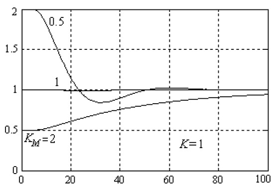
Figure 6. Control responses $c\left(t\right)$ to a unit step setpoint for ${\tau }_M=5$, $T_{sM}=53$ and various $K_M$.

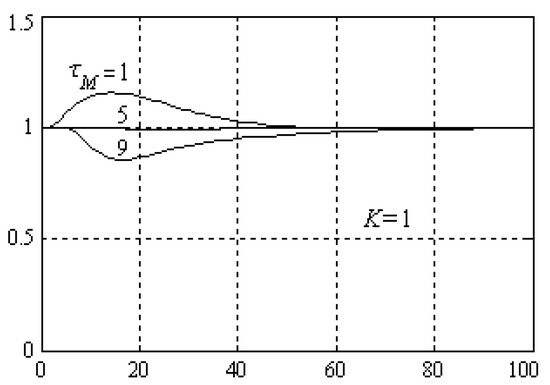
Figure 7. Control responses $c\left(t\right)$ to a unit step setpoint for $K_M=1$, $T_{sM}=53$ and various ${\tau }_M$.

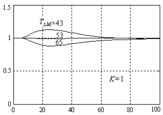
Figure 8. Control responses $c\left(t\right)$ to a unit step setpoint for $K_M=1$, ${\tau }_M=5$ and various $T_{sM}$.

With regard to the closed-loop responses $c\left(t\right)$ to a unit step setpoint in the case $K=1$, the following observations are valid for compensated processes of minimum phase and without overshoot.

• If the initial value $c\left(0_{+}\right)$ differs from the final value $c(\infty )$ (see Figure 6 for $K_M=0.5$ and $K_M=2$), then $K_M$ needs to be multiplied by the ratio $c\left(0_{+}\right)/c(\infty )$.
• If ${\tau }_M$ differs from the compensated process time delay ${\tau }_{P_0}$ (see Figure 7 for ${\tau }_M=1$ and ${\tau }_M=9$), the response $c\left(t\right)$ has a deviation from the step form starting from the time $t=min\{{\tau }_{P_0},{\tau }_M\}$. For $K_{P_0}>0$, the deviation is positive if ${\tau }_M<{\tau }_{P_0}$, and negative if ${\tau }_M>{\tau }_{P_0}$.
• If $K_M\approx K_{P_0}$, ${\tau }_M\approx {\tau }_{P_0}$ and $T_{sM}\ne T_{s{P}_0}$ (see Figure 8 for $T_{sM}=43$ and $T_{sM}=65$), the response $c\left(t\right)$ has a deviation from the step form starting from the time $t={\tau }_M$. For $K_{P_0}>0$, the deviation is positive if $T_{sM}<T_{s{P}_0}$, and negative if $T_{sM}>T_{s{P}_0}$.

In conclusion, if $K=1$ and the closed-loop system response $c\left(t\right)$ to a step setpoint is predominantly larger/smaller than the step function of magnitude $c(\infty )$, then the respective model parameter needs to be suitably augmented/diminished. As a general recommendation, it is better to choose $K_M>K_{P_0}$ than $K_M<K_{P_0}$, ${\tau }_M>{\tau }_{P_0}$ than ${\tau }_M<{\tau }_{P_0}$, and $T_{sM}>T_{s{P}_0}$ than $T_{sM}<T_{s{P}_0}$. For example, if $K_M\approx K_{P_0}$ and ${\tau }_M\approx {\tau }_{P_0}$, then the control performance for $T_{sM}>>T_{s{P}_0}$ and the best tuning gain K (which is greater than 1) is better than that for $T_{sM}<<T_{s{P}_0}$ and the best K (which is less than 1).

5. Two-Degree of Freedom Algorithm

In order to slow down the reference signal, a low pass pre-filter with

$$G_F\left(s\right)=\frac{1}{T_{F}s+1}$$

(41)

can be used. Choosing the time constant

$$T_F=\frac{T_{s95}}{10},$$

(42)

where $T_{s95}$ is the settling time of the closed-loop response $y\left(t\right)$ to a step reference for $T_F=0$, the control responses $c\left(t\right)$ and $u\left(t\right)$ to a step reference have a slower start variation, but that does not cause a significant increase of the settling time of the response $y\left(t\right)$.

6. Illustrative Tests

The control algorithm ${\mathrm{P}}_{\alpha }$-IMC with $\alpha =0.2$ provides a suitable combination between the algorithm with $\alpha =0$ (Figure 1) and the algorithm with $\alpha =1$ (Figure 2). The tests in this section were performed with the algorithm ${\mathrm{P}}_{\alpha }$-IMC for

$$\alpha =0.2,\gamma =1,T_s=T_{s95},$$

i.e., for

$$G_M\left(s\right)=\frac{K_M{e}^{-{\tau }_{M}s}}{{(T_{1}s+1)}^2}$$

(43)

and

$$G_i\left(s\right)=\frac{{(T_{1}s+1)}^2}{K_M{(T_{3}s+1)}^2},$$

(44)

where

$$T_1=\frac{T_{trM95}}{\beta }=\frac{T_{sM95}-{\tau }_M}{4.74},T_3=\frac{T_1}{K_1},K_1=K^{0.4}.$$

(45)

In this case, the discrete-time control algorithm (25) has the particular form:

$$\left\{\begin{array}{c}{e}_k=r_k-y_k\hfill \\ w_k=2p_1{w}_{k-1}-p_1^2{w}_{k-2}+K_M{(1-p_1)}^2(c_{k-1-l_M}-u_0)\hfill \\ f_k=K^{0.2}(e_k-e_0)+w_k\hfill \\ c_k=u_0+2p_3(c_{k-1}-u_0)-p_3^2(c_{k-2}-u_0)+{\displaystyle \frac{K_1^2}{K_M}}(f_k-2q_3{f}_{k-1}+q_3^2{f}_{k-2})\hfill \\ u_k=c_k-K_f(y_k-y_0)\hfill \end{array},\right.$$

(46)

where

$$p_1=e^{-T/T_1},p_3=e^{-T/T_3},q_3=1-\frac{1-p_3}{K_1}.$$

(47)

6.1. P*-Type Proportional Process

Consider the proportional process of P*-type with

$$G_P\left(s\right)=\frac{1.5(2s+1)e^{-6s}}{(6s+1)(10s+1)(15s+1)}.$$

From the process response to a unit step input (Figure 9), one may estimate the following model parameters:

$$K_M=1.5,{\tau }_M=8,T_{sM}=73.$$

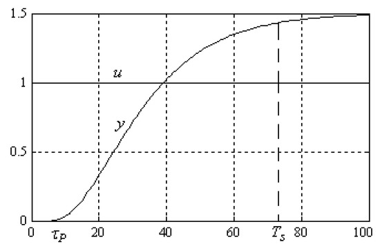
Figure 9. Process response to a unit step input.

Since the process is of proportional type, one selects $K_f=0$, in which case the control variables c and u coincide.

From the responses $y\left(t\right)$ and $u\left(t\right)$ to a unit step reference in Figure 10 and Figure 11, it follows that the control action is suitable for $K=2.4$, slow for $K=1$, too slow for $K=0.5$ and strong for $K=5$. The closed-loop control system remains stable for $0<K<376$.

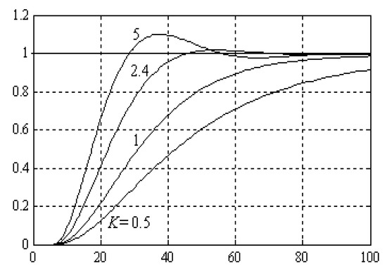
Figure 10. Responses $y\left(t\right)$ to a unit step reference for $K=0.5;1;2.4;5.$

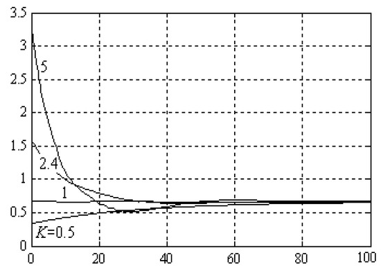
Figure 11. Control responses $u\left(t\right)$ to a unit step reference for $K=0.5;1;2.4;5.$

Since the control response $u\left(t\right)$ for $K=1$ is close to a step function (Figure 11), one can say that the model parameters have been accurately identified, and the model type (43) describes satisfactory the process dynamic.

Figure 12, Figure 13, Figure 14, Figure 15, Figure 16 and Figure 17 highlight the control performance and the robustness of the proposed algorithm with respect to the model parameters.

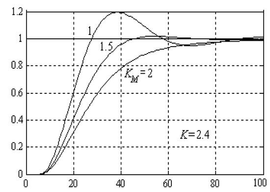
Figure 12. Responses $y\left(t\right)$ to a unit step reference for ${\tau }_M=8$, $T_{sM}=73$ and $K_M=1;1.5;2.$

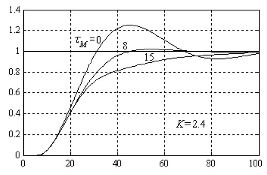
Figure 13. Responses $y\left(t\right)$ to a unit step reference for $K_M=1.5$, $T_{sM}=73$ and ${\tau }_M=0;8;15.$

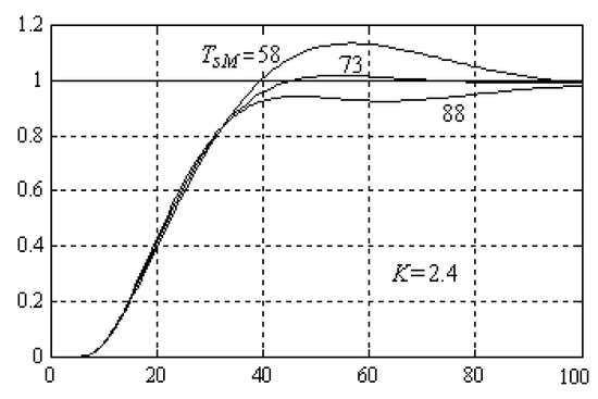
Figure 14. Responses $y\left(t\right)$ to a unit step reference for $K_M=1.5$, ${\tau }_M=8$ and $T_{sM}=58;73;88.$

Figure 15. Responses $y\left(t\right)$ to a unit step reference for: (A) $K_M=2$, $K=6;$ (B) $K_M=1.5$, $K=2.4;$ (C) $K_M=1$, $K=0.5.$

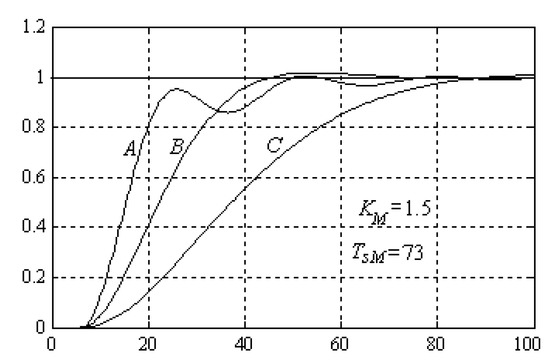
Figure 16. Closed-loop system responses $y\left(t\right)$ to a unit step reference for: (A) ${\tau }_M=15$, $K=7.5;$ (B) ${\tau }_M=8$, $K=2.4;$ (C) ${\tau }_M=0$, $K=0.55.$

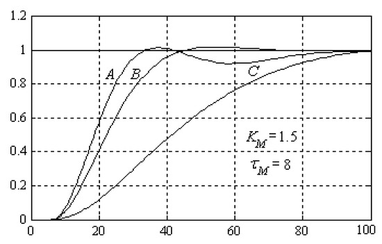
Figure 17. Responses $y\left(t\right)$ to a unit step reference for: (A) $T_{sM}=88$, $K=3.7;$ (B) $T_{sM}=73$, $K=2.4;$ (C) $T_{sM}=58$, $K=0.45.$

Figure 12, Figure 13 and Figure 14 illustrate the responses $y\left(t\right)$ to a unit step reference for $K=2.4$ and various $K_M$, ${\tau }_M$ and $T_{sM}$, respectively. Notice that the three closed-loop control systems are stable for $K_M>0.406$, for ${\tau }_M>0$ and for $T_{sM}>16.5$, respectively. Figure 15, Figure 16 and Figure 17 illustrate the responses $y\left(t\right)$ for various model parameters and a suitable tuning gain K. One can see that if K has an appropriate value, the control performance is preserved even for a wrong setting of the model parameters. The fact that the responses A (where the wrong parameter is greater) are better than the responses C (where the wrong parameter is less) confirms the recommendation in Section 4, that it is better to choose $K_M>K_P$ than $K_M<K_P$, ${\tau }_M>{\tau }_P$ than ${\tau }_M<{\tau }_P$, and $T_{sM}>T_{sP}$ than $T_{sM}<T_{sP}$. In addition, the best tuning gain K is greater than 1 for all responses A and less than 1 for all responses C.

Remark 7.

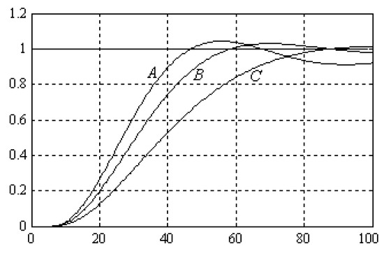
Figure 18 illustrates the closed-loop responses $y\left(t\right)$ to a unit step reference for a PI control algorithm with

$$G_{PI}\left(s\right)=K\left(1+\frac{1}{T_{i}s}\right),$$

in the following cases: A ($K=0.7$ and the suitable $T_i=32$), B ($K=0.5$ and the suitable $T_i=24$) and C ($K=0.3$ and the suitable $T_i=18$). One can see that the best response in Figure 10 (obtained with the proposed algorithm for the suitable $K=2.4$) is better than the best response B in Figure 18 (obtained with the PI algorithm).

Figure 18. Responses $y\left(t\right)$ to a unit step reference for a PI algorithm with: (A) $K=0.7$, $T_i=32;$ (B) $K=0.5$, $T_i=24;$ (C) $K=0.3$, $T_i=18.$

Remark 8.

According to Figure 10, the settling time of the closed-loop response $y\left(t\right)$ to a step reference for the suitable $K=2.4$ is $T_{s95}\approx 40$. Using a reference pre-filter with the time constant (see Section 5)

$$T_F=\frac{T_{s95}}{10}=4,$$

the responses $y\left(t\right)$ and $u\left(t\right)$ in Figure 10 and Figure 11 turn into the responses in Figure 19 and Figure 20, respectively. The responses $y\left(t\right)$ in Figure 19 are comparable with those in Figure 10, whereas the responses $u\left(t\right)$ in Figure 20 have a start variation slower and a maximum value (for $K>1$) less than those in Figure 11.

Figure 19. Responses $y\left(t\right)$ to a unit step reference for $T_F=4$ and $K=0.5;1;2.4;5.$

Figure 20. Control responses $u\left(t\right)$ to a unit step reference for $T_F=4$ and $K=0.5;1;2.4;5.$

6.2. Oscillatory Proportional Process

Consider the oscillatory process

$$G_P\left(s\right)=\frac{1.5(2s+1)e^{-6s}}{(4s+1)(5s+1)(36s^2+2.35s+1)}.$$

From the unit step process response in Figure 21, one gets (see Section 3)

$$K_{\overline{P}}\approx 2,{\tau }_{\overline{P}}=9,t_1=32,$$

therefore

$$K_M=K_{\overline{P}}\approx 2,{\tau }_M={\tau }_{\overline{P}}=9,T_{sM}=T_{s\overline{P}}\approx t_1=32.$$

Figure 21. Process response to a unit step input.

Figure 22 and Figure 23 show the responses $y\left(t\right)$ and $u\left(t\right)$ to a unit step setpoint for the same three values of K. The response $y\left(t\right)$ for $K=0.33$ is satisfactory for the given oscillatory process. Notice that the control system is stable for $0<K<1.5$.

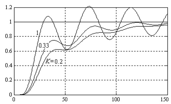
Figure 22. Responses $y\left(t\right)$ to a unit step reference for $K=0.2;0.33;1.$

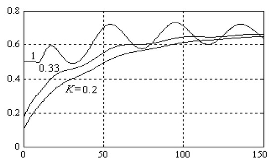
Figure 23. Control responses $u\left(t\right)$ to a unit step reference for $K=0.2;0.33;1.$

6.3. Non-Minimum Phase Process with Overshoot

Consider the non-minimum phase process with overshoot and without oscillations:

$$G_P\left(s\right)=\frac{(30s+1)(-5s+1)e^{-3s}}{(5s+1)(10s+1)(15s+1)}.$$

According to (40) and the unit step process response in Figure 24, we get

$$K_{\overline{P}}=1.23,t_0=10,t_1=35,$$

therefore

$$K_M=K_{\overline{P}}=1.23,{\tau }_M=t_0=10,T_{sM}=T_{s\overline{P}}\approx t_1=35.$$

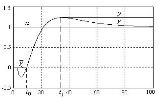
Figure 24. Process response to a unit step input.

Figure 25 and Figure 26 show the responses $y\left(t\right)$ and $u\left(t\right)$ to a unit step setpoint for the same three values of K. Clearly, the best response $y\left(t\right)$ is obtained for $K=1.4$. The control system is stable for $0<K<3.4$.

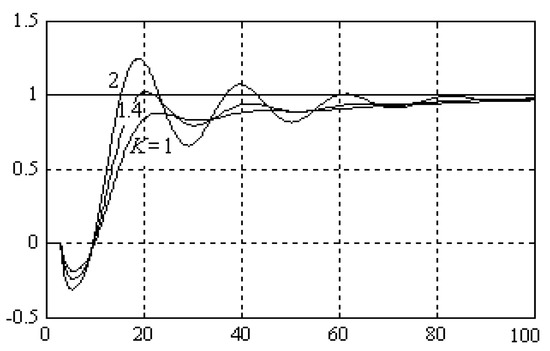
Figure 25. Responses $y\left(t\right)$ to a unit step reference for $K=1;1.4;2.$

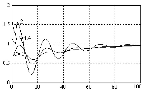
Figure 26. Control responses $u\left(t\right)$ to a unit step reference for $K=1;1.4;2.$

6.4. Integral Process

Consider the integral process with time delay:

$$G_P\left(s\right)=\frac{3(2s+1)e^{-6s}}{40s(3s+1)(4s+1)}.$$

For $0<K_f<0.45$, the compensated process is of P*-type (Figure 27), with a monotone and bounded response to a step input. Choosing $K_f=0.4$, the compensated process model has the parameters

$$K_M=2.5,{\tau }_M=7,T_{sM}=70,$$

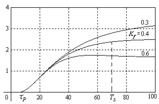
Figure 27. Compensated process responses to a unit step input.

The responses $y\left(t\right)$, $c\left(t\right)$, and $u\left(t\right)$ to a unit step setpoint are respectively shown for the same three values of K in Figure 28, Figure 29 and Figure 30. The response $y\left(t\right)$ for $K=3.3$ (Figure 28) is very good for the given integral process. Since the control response $c\left(t\right)$ for $K=1$ is close to a step shape (Figure 29), the model type (43) describes with sufficient accuracy the compensated process sluggishness. The closed-loop control system is stable for $0<K<110$.

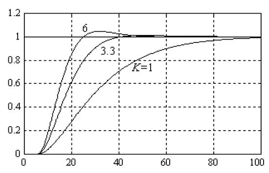
Figure 28. Responses $y\left(t\right)$ to a unit step setpoint for $K=1;3.3;6.$

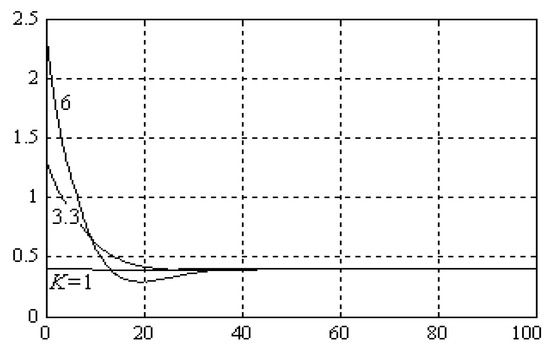
Figure 29. Control responses $c\left(t\right)$ to a unit step setpoint for $K=1;3.3;6.$

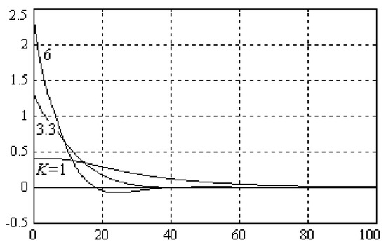
Figure 30. Control responses $u\left(t\right)$ to a unit step setpoint for $K=1;3.3;6.$

Figure 31 shows for $K=3.3$ the responses $y\left(t\right)$ to a step and ramp disturbance v. Notice that the steady-state error is zero for any step and ramp disturbance.

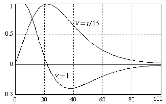
Figure 31. Responses $y\left(t\right)$ to a step and ramp disturbance.

6.5. Unstable Process

Consider the unstable process

$$G_P\left(s\right)=\frac{3e^{-2s}}{2(4s+1)(10s-1)}.$$

Using a negative feedback path with $0.667<K_f<0.75$, the process turns into a compensated process of P*-type having a monotone and bounded response to a step input (Figure 32). By selecting $K_f=0.74$, the model of the compensated process has the following parameters:

$$K_M=13.8,{\tau }_M=4,T_{sM}=80.$$

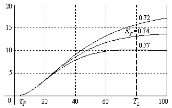
Figure 32. Compensated process responses to a unit step input.

The responses $y\left(t\right)$, $c\left(t\right)$, and $u\left(t\right)$ to a unit step setpoint are shown in Figure 33, Figure 34 and Figure 35 for the same three values of K. Since the control response $c\left(t\right)$ is close to a step shape for $K=1$ (Figure 34), the model (43) describes with accuracy the compensated process dynamic. The closed-loop control system is stable for $0<K<410$.

Figure 33. Responses $y\left(t\right)$ to a unit step setpoint for $K=1;1.5;4.$

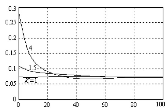
Figure 34. Control responses $c\left(t\right)$ to a unit step setpoint for $K=1;1.5;4.$

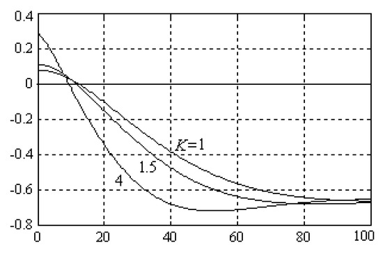
Figure 35. Control responses $u\left(t\right)$ to a unit step setpoint for $K=1;1.5;4.$

7. Conclusions

The paper addresses a practical unified control algorithm which, due to the control performance, robustness to modeling error and process uncertainties, and capacity to be easily tuned and used for all industrial plants, could be a real alternative to the known PID algorithm.

The proposed algorithm is a suitable trade-off between the known P0-IMC algorithm and P1-IMC algorithm, which provide a too weak and a too strong impact of the tuning gain K on the control action, respectively. The P-IMC algorithm is better than the PID algorithm with respect to both the tuning procedure simplicity and the control performance (especially for processes of non-minimum phase or/and with time delay), and is more efficient than the IMC algorithm due to the stronger and safer influence of the component P on the control action.

The algorithm has five parameters: The process feedback gain $K_f$ (used to turn integral or unstable processes into a stable proportional compensated process), the tuning gain K (used to adjust the control intensity), and three parameters of the compensated process model: Steady-state gain, time delay, and settling time. All parameters of the P-IMC algorithm can be determined experimentally. By choosing a suitable K, the reference tracking performance is satisfactory even for a large uncertainty of the model parameters. However, as a general recommendation, it is desirable that the value of a parameter of the compensated process model to be selected equal or larger than its real value. For such a larger selection, the best tuning gain K is usually more than 1, and the control performance is better than for a smaller selection (when the best K is less than 1).

There is a simple procedure to check and correct online the model parameters through simple visual analysis of the shape of the internal controller response to a step reference. This procedure is based on the step control principle, which states that for $K=1$ and a perfect model, the internal controller response to a step reference has a step shape. Thus, by analyzing the deviation of the internal controller response from the step shape, the model parameters can be suitably adjusted to improve the model accuracy.

If the steady-state gains of the model and the compensated process are equal to each other, the initial value of the internal controller response to a step reference is K times its final value. This feature enables the human operator to select the tuning gain K and understand better its role in the control action.

Since the proposed P-IMC algorithm can be implemented in practice only in discrete-time, it is designed in both continuous-time and discrete-time.

For $\alpha =0.2$ and $\gamma =1$ (i.e., $T_1=T_2$), the P-IMC algorithm has been tested in real time, with excellent results, in laboratory and field conditions. In the future, interesting comparative research and control applications based on the P-IMC algorithm could be made in chemistry and allied engineering fields.

References

- Marlin, T. Process Control—Designing Processes and Control Systems for Dynamic Performance; McGraw Hill: New York, NY, USA, 1995. [Google Scholar]
- Brosilow, C.; Joseph, B. Techniques of Model-Based Control; Prentice Hall: Upper Saddle River, NJ, USA, 2001. [Google Scholar]
- Almabrok, A.; Psarakis, M.; Dounis, A. Fast tuning of the PID Controller in an HVAC system using big bang-big crunch algorithm and FPGA technology. Algorithms 2018, 11, 146. [Google Scholar] [CrossRef]
- Ang, K.H.; Chong, G.; Li, Y. PID control system analysis, design, and technology. IEEE Trans. Control Syst. Technol. 2005, 13, 559–576. [Google Scholar]
- Firouzbahrami, M.; Nobakhti, A. Reliable computation of PID gain space for general second-order time-delay systems. Int. J. Control 2017, 90, 2124–2136. [Google Scholar] [CrossRef]
- Berner, J.; Soltesz, K.; Hagglund, T.; Astrom, K. An experimental comparison of PID autotuners. Control Eng. Pract. 2018, 73, 124–133. [Google Scholar] [CrossRef]
- Wang, S.; Yan, X.; Li, D.; Sun, L. An Approach for Setting Parameters for Two-Degree-of-Freedom PID Controllers. Algorithms 2018, 11, 48. [Google Scholar] [CrossRef]
- Wu, Z.; Li, D.; Xue, Y. A New PID Controller Design with Constraints on Relative Delay Margin for First-Order plus Dead-Time Systems. Processes 2019, 7, 713. [Google Scholar] [CrossRef]
- Francis, B.; Wonham, W. The internal model principle of control theory. Automatica 1976, 12, 457–465. [Google Scholar] [CrossRef]
- Bengtsson, G. Output regulation and internal models. A frequency domain approach. Automatica 1977, 13, 333–345. [Google Scholar] [CrossRef]
- Garcia, C.; Morari, M. Internal model control—A unifying review and some new results. Ind. Eng. Chem. Proc. Des. Dev. 1982, 21, 308–323. [Google Scholar] [CrossRef]
- Horn, I.; Arulandu, J.; Gombas, C. Improved filter design in internal model control. Ind. Eng. Chem. Res. 1996, 35, 3437–3441. [Google Scholar] [CrossRef]
- Zazueta, S.; Alvarez, J. Stability robustness and practical implementation of an internal model control structure. Eur. J. Control 2000, 6, 268–278. [Google Scholar] [CrossRef]
- Liu, T.; Gao, F. New insight into internal model control filter design for load disturbance rejection. IET Control Theory Appl. 2010, 4, 448–460. [Google Scholar] [CrossRef]
- Saxena, S.; Hote, Y. Advances in internal model control technique: A review and future prospects. IETE Tech. Rev. 2012, 29, 461–472. [Google Scholar] [CrossRef]
- Muresan, C.; Dutta, A.; Dulf, E.; Pinar, Z.; Maxim, A.; Ionescu, C. Tuning algorithms for fractional order internal model controllers for time delay processes. Int. J. Control 2016, 89, 579–593. [Google Scholar] [CrossRef]
- Rivera, D.; Morari, M.; Skogestad, S. Internal model control-PID controller design. Ind. Eng. Chem. Process Des. Dev. 1986, 25, 252–265. [Google Scholar] [CrossRef]
- Leva, A. Performance and robustness improvement in the IMC-PID tuning method. Eur. J. Control 2006, 12, 195–204. [Google Scholar] [CrossRef]
- Santosh-Kumar, D.B.; Padma-Sree, R. Tuning of IMC based PID controllers for integrating systems with time delay. ISA Trans. 2016, 63, 242–255. [Google Scholar] [CrossRef]
- Cirtoaje, V. A quasi-universal practical IMC algorithm. Automatika 2017, 58, 168–181. [Google Scholar] [CrossRef][Green Version]
- Cirtoaje, V.; Baiesu, A. On a model based practical control algorithm. Stud. Inform. Control 2018, 37, 83–96. [Google Scholar] [CrossRef]
- Tan, W.; Marquez, H.J.; Chen, T. IMC design for unstable processes with time delays. J. Process Control 2003, 13, 203–213. [Google Scholar] [CrossRef]
- Shibasaki, H.; Endo, J.; Hikichi, Y.; Tanaka, R.; Kawaguchi, K.; Ishida, Y. A modified internal model control for an unstable plant with an integrator in continuous-time system. Int. J. Inf. Electr. Eng. 2013, 3, 357–360. [Google Scholar]
- Cirtoaje, V. Process compensation based control. Bul. Univ. Petr. Gaze din Ploiesti-Ser. Teh. 2006, LVIII, 48–53. [Google Scholar]
© 2020 by the author. Licensee MDPI, Basel, Switzerland. This article is an open access article distributed under the terms and conditions of the Creative Commons Attribution (CC BY) license (http://creativecommons.org/licenses/by/4.0/).