Abstract
To address the decline in system inertia and the risk of frequency instability resulting from high penetration of renewable energy, and to overcome the limitations of centralized control—such as high computational burden and slow response—as well as the lack of global coordination in decentralized control, this study proposes a cooperative decision-making strategy, based on system partitioning, for high-frequency generator tripping control. The method first combines spectral clustering with nodal frequency response correlation analysis to achieve dynamic system partitioning and the selection of characteristic monitoring nodes. A two-layer cooperative architecture consisting of zone controllers and a central controller is then established, in which the zone controllers are responsible for aggregating local information, while the central controller dynamically generates a zonal generator tripping priority sequence based on four indicators: regional power surplus ratio, equivalent inertia, frequency deviation, and Rate of Change of Frequency. A simulation study conducted on an actual provincial power grid in the northwest region with a renewable energy penetration rate of 31.1% showed that compared with the existing decentralized control strategy of the power grid, this method not only achieved better frequency recovery, but also reduced the generator tripping capacity by 6.29%. Compared with advanced centralized strategies, it reduces recovery time by 10% while achieving good frequency recovery. By aggregating regional information to reduce central computing load and implementing coordinated control between regions through a global optimization mechanism, this strategy provides an effective method for high-frequency safety control in power grids with high penetration rates of renewable energy.
1. Introduction
As the “dual carbon” goals advance, the continuous growth in installed capacity and grid penetration of renewable energy sources like wind and solar power has led to a gradual decrease in the system’s equivalent inertia [1,2,3]. This trend significantly exacerbates frequency security issues during high-power disturbances. High-frequency generator tripping technology, serving as a core measure within the grid’s third line of defense, provides a critical safeguard against frequency instability during extreme fault conditions.
Extensive research has been conducted on high-frequency stability issues in power systems, with a primary focus on regional partitioning, control strategies, and generator tripping schemes. In terms of system partitioning, spectral clustering-based methods have been proposed to strengthen intra-regional electrical connectivity and dynamic consistency [4], while shared regional partitioning metrics have enabled finer-grained segmentation of transmission networks [5]. However, these approaches often neglect operational safety constraints or rely on parameters that are difficult to obtain in practice, thereby limiting their engineering applicability. Regarding generator tripping strategies, various methods have been developed to balance control effectiveness and computational efficiency. Approaches based on local load information reduce communication requirements but may fail to account for computational complexity constraints [6]. Dual-threshold generator tripping termination criteria improve execution efficiency but may result in excessive generator disconnections under severe disturbances [7]. More comprehensive schemes employing exhaustive time-domain simulations and parallel multiprocessor computation can account for multi-factor disturbances, albeit with limited strategy diversity and increased computational burden [8]. Sub-synchronous oscillation identification methods based on amplitude–frequency dual-dimensional criteria have also been proposed to implement differentiated generator tripping control, enhancing transient stability margins under specific oscillatory conditions [9], while time-domain analysis-based high-frequency cut-off optimization schemes lack explicit generator tripping calculation mechanisms [10]. Data-driven optimization strategies, such as those based on random forest algorithms, reduce the number of tripped units but suffer from high iteration requirements that adversely affect real-time performance [11]. Centralized forecasting-based frequency regulation models further improve primary frequency control capability, yet their effectiveness remains constrained by forecasting accuracy [12]. Hierarchical and multi-level control architectures have been widely investigated to enhance coordination in large-scale systems [13,14]. However, their multi-layer structures can introduce delays and reduce control efficiency under fast frequency disturbances. In addition, recent studies have explored communication-assisted coordination mechanisms and advanced control strategies for renewable-dominated power systems, improving system flexibility and transient stability under specific operating scenarios [15,16].
In traditional power systems dominated by synchronous generators, during high-frequency faults, the rotational inertia of synchronous generator rotors can buffer system power imbalances through kinetic energy release and absorption, providing ample response windows for high-frequency generator tripping measures based on electromechanical response mechanisms. However, the large-scale grid integration of renewable energy units such as wind and solar power has rendered the system low-inertia, causing its frequency change rate to increase severalfold compared to traditional systems. Against this backdrop, traditional high-frequency generator tripping strategies face dual adaptability challenges in new power systems with high renewable energy penetration. On the one hand, there exists a temporal adaptability mismatch between the rapid frequency dynamics and the response speed of conventional generator tripping strategies. Under low-inertia operating conditions, a sudden power imbalance may cause the system frequency to rise sharply with a high Rate of Change of Frequency (RoCoF, all abbreviations and full names in the text are listed in Appendix A Table A1). However, traditional strategies rely on sequential processes including frequency measurement, threshold-based decision-making, and command execution, which often lag behind the fast frequency evolution and thus fail to suppress the frequency peak in a timely manner. On the other hand, there is a structural adaptability mismatch between traditional control targets and the physical characteristics of modern power systems. Conventional high-frequency generator tripping strategies are primarily designed for centralized synchronous generators, whereas renewable generation units are typically dispersed, connected at multiple grid nodes, and exhibit limited controllability. In such scenarios, tripping synchronous generator alone may not achieve the expected frequency regulation effect. Moreover, large-scale and disorderly disconnection of renewable units triggered by protection mechanisms may further aggravate the system power imbalance, potentially increasing the risk of frequency collapse. These dual adaptability challenges indicate that traditional frequency control strategies, which are fundamentally rooted in the physical principles of synchronous machines, are increasingly ill-suited to the dynamic operational characteristics of new power systems. Consequently, there is an urgent need to overcome the limitations of conventional generator tripping methods and to develop high-frequency stability control approaches that are better adapted to systems with high renewable energy penetration.
To address the aforementioned challenges, this study proposes a partition-based cooperative decision-making strategy for high-frequency generator tripping control. Compared with existing zonal-hierarchical control methods, the main contributions of this paper are summarized as follows:
- (1)
- A dynamic system partitioning and representative-node selection method is proposed by integrating spectral clustering with nodal frequency response correlation analysis. Compared with traditional static zoning approaches, the proposed method better captures the dynamic electrical coupling characteristics of low-inertia power systems and improves the accuracy of regional frequency perception.
- (2)
- A lightweight two-layer cooperative decision-making architecture consisting of zone controllers and a central controller is developed. Different from conventional centralized or fully decentralized generator tripping schemes, this architecture significantly reduces computational and communication burdens while preserving global coordination capability.
- (3)
- A comprehensive regional prioritization model for high-frequency generator tripping is established by integrating four key indicators, including regional power surplus ratio, equivalent inertia time constant, frequency deviation, and RoCoF. By adopting a data-driven AHP-based weighting strategy, the proposed model effectively avoids over-tripping and under-tripping risks under high renewable energy penetration scenarios.
Through these systematic innovations, this study provides a new solution for high-frequency security and stability control in power grids with high penetration of renewable energy.
2. System Partition
This section proposes a dynamic region partitioning and representative node selection method based on spectral clustering algorithm and node frequency response correlation. Compared with traditional static zone partitioning methods, this method can adapt to changes in system electrical coupling, thereby significantly improving the accuracy of zone frequency monitoring.
2.1. Power System Partitioning Based on Spectral Clustering Algorithms
Traditional power system zoning primarily relies on geographic topology constraints or dispatchers’ heuristic rules, making it difficult to meet the refined requirements for regional structural consistency in modern complex power grids. Due to the fact that the power system can be represented in the form of a weighted graph, this study adopts a spectral clustering algorithm based on graph theory [17] to partition the system into regions. Unlike traditional clustering algorithms that rely on geometric distances in the original feature space, graph theory based spectral clustering algorithms utilize the spectral properties of Laplacian matrices to project system nodes into a low dimensional feature vector space, thereby avoiding the limitations of traditional methods that are sensitive to initialization and easy to converge to local optima. By using electrical distance as a measure of node similarity, consequently, the resulting partitions exhibit stronger intra-regional aggregation and weaker inter regional coupling. This enables the partitioning results to more accurately characterize the dynamic electrical structural characteristics of the power grid, especially the consistency of frequency response behavior between different regions, and increases the accuracy of subsequent partitioning parameter measurements.
Through graph theory, the power system can be modeled as a weighted undirected graph , where the vertex set is the set of n nodes in the system, and the edge set E represents the set of power transmission channels between nodes. The edge weight function represents the strength of electrical coupling between nodes, and the degree of coupling is positively correlated with the edge weight value. Through the study of electrical distance measurement of line impedance and transmission power [18], this study innovatively defines a static edge weight model , as shown in Equation (1). This static edge weight avoids the sensitivity of traditional dynamic edge weights to power flow and ensures that partition results remain stable under system interference. From the perspective of network algebra, this edge weight is essentially a topological mapping of the admittance matrix [19], which can accurately represent the static internal structure of the power grid. The region partitioning results obtained using this method satisfy the criterion of minimizing node frequency variance, and compared with the entire network, the frequency consistency within the region is significantly improved.
where and represent the line resistance and reactance between nodes i and j, respectively.
The system partitioning flowchart is shown in Figure 1. First, construct an adjacency matrix representing the electrical distances between nodes in the system graph, where the edge weights are the reciprocal impedances. Subsequently, build the Laplacian matrix [18] from the adjacency matrix and normalize it as shown in Equation (2). The core concept of the spectral clustering algorithm is to treat data as a graph structure. By performing spectral decomposition on the graph’s Laplacian matrix, the original data is mapped to a low-dimensional space via eigenvectors. This reduces the matrix order and ultimately achieves clustering partitioning.
where , .
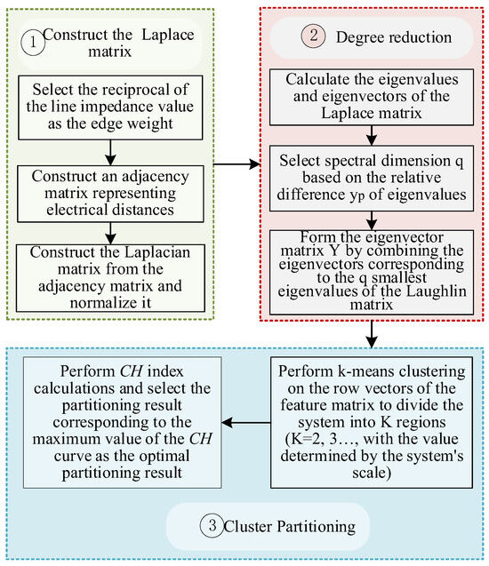
Figure 1.
System Partitioning Flowchart.
For matrix , determine the eigenvectors corresponding to each eigenvalue. Calculate the eigenvalue gap [20] between two eigenvalues using Equation (3). Select the spectral embedding dimension q based on the maximum eigenvalue gap. Perform eigenvalue decomposition on the Laplacian matrix to obtain the eigenvectors corresponding to the first q eigenvalues, and arrange them in columns to form the eigenvector matrix. Finally, cluster analysis is performed on the row vectors of the matrix to obtain the regional partitioning results.
where is the pth normalized eigenvalue of the matrix; is the (p+1)th normalized eigenvalue of the matrix.
Finally, k-means clustering is employed to enhance the clustering outcome [18]. The optimal number of partitions for the k-means clustering algorithm is determined by the Calinski–Harabasz (CH) index [20], and the output result is the partition corresponding to each node.
where k is the number of clustering partitions; n is the total number of nodes in the entire network; is the set of nodes in the i-th partition; is the cardinality of nodes in partition i; is the centroid of the feature vectors after partitioning; is the mean of the feature vectors across the entire network.
The CH index takes into account both the Within-Group Sum of Squares (WGSS) and the Between-Group Sum of Squares (BGSS), and can be used to evaluate the quality of the clustering. The larger the CH value, the better the clustering results. Specifically, clustering results obtained under representative operating conditions are assessed for different candidate partition numbers, and the partition configuration corresponding to the maximum CH index value is identified as the optimal solution. Once determined, the partition structure is fixed and directly applied during online operation, where only zonal measurements and cooperative decision-making are performed. This design ensures a low computational burden in real-time operation and supports the practical feasibility of the proposed method.
2.2. Selection of Regional Frequency Measurement Points
In power systems, electromechanical transient processes triggered by disturbances—such as load changes, generator tripping, or short-circuit faults—are fundamentally characterized by the interaction between generator rotor mechanical motion and grid electromagnetic power. This phenomenon results in spatially heterogeneous frequency responses, with strong correlations existing only in regions of high electrical coupling. To more accurately determine regional frequency variations and avoid errors from randomly selected measurement points, it is necessary to select the most representative nodes in each region as frequency measurement points.
The selection of regional frequency measurement points should ensure that the monitored data effectively represent the overall frequency dynamic response of the region [20]. To this end, this study adopts the Pearson correlation coefficient to quantify the similarity of nodal frequency responses and thereby selects representative measurement points for each region. The Pearson correlation coefficient is a statistical measure of the linear correlation between two variables, with values ranging from [−1, 1]; an absolute value closer to 1 indicates a stronger linear correlation. By applying disturbances to the system and collecting frequency response data, a Pearson correlation matrix R [18] of the nodal frequency responses is calculated. The matrix element Rij defined by Equation (7), represents the Pearson correlation coefficient between the measured frequency data of node i and node j, which is equal to the ratio of the covariance of the two variables to the product of their standard deviations. Furthermore, a similarity index Ci [18] for node i is defined as shown in Equation (8), reflecting the average correlation between the frequency response of that node and all other nodes in the same region. Within each region, all nodes are ranked in descending order according to their similarity index Ci. The node with the largest is designated as the region’s node. The frequency response of this node exhibits the highest overall similarity to the responses of other nodes within the region and can therefore accurately reflect the regional frequency dynamics. Based on the above analysis, the node in each region is ultimately selected as its frequency measurement point.
where denotes the covariance between the frequency response sequences at nodes i and j; and represent the frequency response sequences at nodes i and j, respectively; and denote the standard deviations of the frequency response sequences at nodes i and j, respectively; and denote the mth values of the frequency response sequences at nodes i and j, respectively; and denote the mean values of the frequency response sequences at nodes i and j, respectively; M is the sample size of the frequency response sequence; Nb is the total number of nodes.
In order to eliminate disturbances and environmental impacts, multiple disturbance condition tests were conducted on the system, and the node with the strongest anti-interference ability was selected as the node in the region. The position of this node can serve as a parameter measurement point for the regional controller. The method proposed in this section aims to measure the frequency changes after system failures more quickly and accurately, and upload them to the central controller for data analysis. This method performs full-zone data analysis relative to centralized generator tripping control approaches. Its advantage lies in the fact that the central processor only needs to analyze Cmax node data from each zone, significantly reducing data processing time and thereby minimizing the impact of communication delays on generator tripping performance.
3. System Inertia Theory and Unbalanced Power Calculation
3.1. Inertia Calculation Based on Local Load Information
The inertia in the power system is essentially the kinetic energy stored in the rotating mass of the synchronous generator. Its physical characteristics manifest as the inherent ability of the system to resist frequency changes. When disturbances occur causing power imbalance, the system frequency deviates from its rated value. During this transient process, the rotational inertia of the synchronous generator responds instantaneously through its mechanical inertia. By converting kinetic energy into electrical energy, they will automatically release or absorb some of the stored kinetic energy, thereby compensating for short-term power shortages or surpluses. This process significantly reduces the initial RoCoF, providing a critical response time window for frequency control measures. Therefore, the inertia level of the system is one of the core physical parameters that determine frequency stability [19]: higher inertia levels result in lower system RoCoF and stronger frequency stability; conversely, insufficient inertia exacerbates frequency fluctuations and significantly increases the risk of system instability.
The rotational characteristics of a generator rotor can be described by differential equations [1]:
where M, Pm, Pe, ωr, ωs, D, ΔP represent the rotor inertia, mechanical power, electromagnetic power, actual rotor angular velocity, synchronous rotor angular velocity, damping coefficient, and imbalance power, respectively.
By further reasoning from Equation (9), the formula for calculating the system unbalanced power is as follows:
where is the system equivalent inertia; is the system center of inertia frequency; is the system unbalanced power; is the inertia of the i-th generator.
When there is a significant interference such as N-1 short circuit fault or DC bus lockout in the system, power imbalance can cause frequency rise. Once the frequency reaches the threshold of the high-frequency generator trip device, the generator trip operation will be triggered. This will remove excess generator sets to restore power balance, thereby restoring the system to a stable operating state [21,22,23]. represents the moment when the first round of generator trips, and at time , a portion of the critical generators in the system will be cut off. t1 and t2 correspond to two adjacent moments before and after time t. According to Equation (10), it can be inferred that:
where and represent the centers of inertia RoCoF at times t1 and t2, respectively; and [24] denote the system unbalanced power at times t1 and t2.
where , , represent the active power, mechanical active power, and losses of the system load at time t1; , , represent the active power, mechanical active power, and losses of the system load at time t2.
By subtracting (14) from (13), it can be noted that, constrained by generator inertia, the variation in mechanical power remains negligible over a short time scale. In addition, due to the inherent characteristics of system losses, the short-term variation in the loss term is also very small. Within the time interval (t1, t2), the variation in active power of system loads is significantly larger than those of and ; therefore, these two terms can be neglected. Consequently, (17) and (18) are obtained:
Since the parameters in Equation (18) can be measured by local measurement devices, a method for calculating the system inertia is obtained.
This further yields the unbalanced power calculation formula based on the virtual equivalent inertia of load nodes, as shown in Equations (19) and (20) [25].
where is the redundant power of the system at time t = ti; is the frequency derivative function at load node j at time t = ti; is the equivalent inertia of load node j.
By comparing the right-hand sides of the previous two equations, we obtain
Since the center frequency of inertia can be approximated as the center frequency of the load, the following equation is derived [26]:
The equivalent moment of inertia for the jth load node, calculated based on load node information:
where and represent the active power of load node j at times t1 and t2, respectively.
3.2. Unbalanced Power Calculation
According to Equation (19), by substituting the virtual equivalent inertia of the system with that of the load node, a formula for calculating the unbalanced power of each load node is derived.
The static characteristics of the load are as follows [4]:
where is the active power of the load at time t; is the initial active power of the load before disturbance; U is the actual voltage at the load node; U0 is the rated voltage of the load; is the frequency deviation; f0 is the rated frequency of the system; is the active-frequency characteristic coefficient, representing the percentage change in active power with frequency variation; is the active-voltage characteristic index, reflecting the sensitivity of active power to voltage changes.
When the system experiences disturbances due to external interference, the initial frequency changes are minimal. Consequently, the impact on load active power is negligible, meaning changes in load active power primarily depend on voltage variations. Define the active power surplus caused by voltage deviation at the jth load node from the disturbance onset at time t = t0 – t0 time t = T as [27]:
Using Equation (24), the unbalanced power at load node j at time t = t1 can be calculated. By adding the active power redundancy caused by voltage offset via Equation (26), the total active power redundancy at this load node at time t = t1 is obtained. Based on Equations (24) and (26), the power redundancy at load node j at time t = t1 is calculated as follows:
4. Priority Selection Criteria for Cutting Machine Zones
This section establishes a comprehensive regional assessment model that integrates four types of indicators: power, inertia, frequency deviation, and rate of change. The weights are applied through the Analytic Hierarchy Process [24]. This model overcomes the limitations of traditional approaches that rely on single indicators, making it particularly suitable for operating scenarios characterized by strong renewable energy fluctuations and low system inertia.
4.1. Power Distribution and Inertia Parameters
4.1.1. Regional Power Surplus Ratio
The regional excess power ratio serves as a key metric for assessing a specific region’s contribution to the overall power imbalance within the system. It is defined as the percentage of the region’s actual excess power relative to the system’s total excess power. This contribution can be quantified through normalization methods. Regions exhibiting higher contribution ratios are typically regarded as primary disturbance sources and should be prioritized for elimination to rapidly reduce system redundant power. The formula is as follows [28]:
where is the net excess power of region i; is the sum of the net excess power across all regions.
4.1.2. Equivalent Inertial Time Constant
The equivalent inertia time constant is a key parameter for assessing the ability of a power system or a specific region to resist power disturbances. Its physical essence lies in characterizing the comprehensive capability of the system to maintain frequency stability through the synergistic effect of physical rotating inertia and virtual inertia. This parameter integrates the actual inertia of rotating equipment such as synchronous generators with the virtual inertia emulated by power electronic devices through control strategies. Zones with lower inertia levels exhibit weaker resistance to frequency fluctuations and thus should be assigned higher priority in generator tripping decisions. Particularly in scenarios with high penetration of renewable energy, the dynamic response characteristics of virtual inertia must be incorporated into the equivalent inertia evaluation to accurately quantify the system’s true disturbance rejection capability.
Its calculation formula is given as follows [25]:
where represents the physical inertia component; represents the virtual inertia component; denotes the rotational inertia of the kth synchronous unit; represents the synchronous angular velocity; denotes the virtual inertia energy; represents the power response of the virtual inertia device at time t.
To more precisely characterize the virtual inertia contributions from different renewable energy technologies, this study refines the modeling for Photovoltaic (PV) inverters and doubly fed induction generator (DFIG) as follows [25]:
- 1.
- Virtual Inertia from PV Systems
For PV inverters whose supplementary power control is triggered by the RoCoF, the equivalent virtual inertia time constant can be modeled as:
where is the equivalent inertia of the PV unit; is the rated capacity of the PV unit; is the differential gain coefficient of the PV virtual inertia control; t is the inertia response time of the PV unit after being subjected to a disturbance; is the maximum frequency deviation during the response period.
- 2.
- Virtual Inertia from DFIG
For DFIG that provide short-term power support by releasing rotor kinetic energy, the equivalent virtual inertia time constant can be expressed as:
where is the inertia time constant of a single unit in the wind turbine cluster; is the change in the rotor angular speed of the wind turbine; is the change in the synchronous angular speed of the unit; is the synchronous angular speed of the system under the initial condition; is the initial rotor angular speed of the wind turbine; is the rated angular speed of the wind turbine; is the inherent inertia time constant of the wind power system.
4.2. Frequency Dynamic Characteristics Parameters
4.2.1. Frequency Deviation
Frequency deviation Δf serves as the core parameter for measuring regional power imbalance during high-frequency faults in power systems. It fundamentally reflects the direct impact of real-time power imbalances between generation and load on system frequency. Frequency deviation directly quantifies the matching state between regional generation capacity and load demand. When system power surplus occurs, the excess power converts into rotational kinetic energy of generator rotors, causing frequency to rise. A larger frequency deviation indicates more significant power redundancy in the region. Failure to promptly trip excess generators will trigger sustained frequency escalation, threatening equipment safety and system stability. As an intuitive representation of power imbalance severity, frequency deviation serves as the primary dynamic indicator for selecting priority generator tripping zones. Its formula is as follows [28]:
where is the actual frequency value at time t; is the system’s rated frequency value. > 0 indicates the system frequency exceeds the rated value, typically caused by excess power; < 0 indicates the system frequency falls below the rated value, typically caused by power deficiency.
4.2.2. Rate of Change of Frequency
RoCoF is a key dynamic metric for measuring the rate of frequency fluctuations in power systems, fundamentally reflecting the system’s inertia capacity for instantaneous response to power disturbances. RoCoF embodies the buffering capability of system inertia against power disturbances. In regions with low inertia levels, excess power can trigger extremely high RoCoF, necessitating priority disconnection of power sources to prevent system instability. Its calculation relies on the dynamic relationship between power imbalance and equivalent inertia—lower inertia yields more severe RoCoF, demanding higher timeliness in generator disconnection responses. In high-frequency fault scenarios, RoCoF serves as one of the core parameters for selecting priority disconnection zones.
The theoretical calculation formula is as follows [29]:
where is the power imbalance quantity, > 0 indicates excess generation, and < 0 indicates a power deficit; is the system’s equivalent inertia time constant; is the system’s base capacity; this equation is derived from the relationship between power imbalance and system inertia.
Due to the difficulty in calculating system power imbalance, the following formula is generally used for calculation [29].
where is the system frequency at time t; is the system frequency at time ; is the sampling time interval; this equation is calculated based on the frequency time series.
4.3. Regional Composite Indicator
In summary, the indicator system for selecting the generator tripping zone in the system consists of four parts: regional power surplus rate, equivalent inertia time constant, frequency deviation, and RoCoF. In order to eliminate dimension differences between various parameters, each indicator needs to be normalized. This article uses the range method for normalization, as shown in the following equation [4]:
where is the original value of the jth parameter for region i; and are the minimum and maximum values of the jth parameter across all regions, respectively; is the normalized parameter value.
The selection of the generator tripping zone comprehensively considers four indicators: regional power surplus ratio, equivalent inertia time constant, frequency deviation, and frequency change rate. This study employs the unified objective method to convert these four indicators into a single composite indicator, assigning corresponding weights to each to reflect their relative importance. The regional composite indicator is expressed as follows [4]:
where is the regional composite indicator; , , and denote the normalized values of regional power surplus ratio, equivalent inertia time constant, frequency deviation, and RoCoF, respectively; , , , and are the weighting factors for the indicators.
4.4. Calculation of Indicator Weights Based on Analytic Hierarchy Process
In the proposed methodology, the AHP is adopted to determine the weights of multiple performance indicators involved in high-frequency generator tripping. Below, I will provide a detailed introduction to the principles of Analytic Hierarchy Process [30]. The schematic diagram of this method is shown in Figure 2. Decision-making problems can be divided into three fundamental levels: the top level is the objective layer, which defines core goals and directions; the middle layer is the criterion layer, encompassing specific dimensions and evaluation indicators required to achieve objectives, forming a multidimensional assessment system; the bottom layer is the solution layer, providing specific action plans or decision objects for selection.
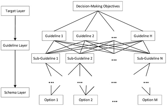
Figure 2.
Model of analytic hierarchy process.
Moreover, weights should be set by considering both the significance of indicators and their interrelationships. The weight determination can be performed offline with low computational burden, which is suitable for real-time emergency control applications. AHP provides a transparent and structured framework to quantify these relative importance relationships, while avoiding heuristic parameter tuning.
By using the Analytic Hierarchy Process to score each indicator, the expert decision-making system obtains the judgment matrix A through specific models and fault types. The eigenvectors corresponding to the maximum eigenvalue of the judgment matrix are solved and normalized to obtain the weights of each indicator. Therefore, the weight of each indicator obtained through the judgment matrix is most suitable for the model and the current fault situation [31]. According to Table 1, the proposed method first assigns appropriate weights to each indicator, and then uses linear weighting to calculate the comprehensive indicator value of the region. Finally, the system sorted the generator tripping zones based on the size of the comprehensive indicator values, achieving the optimal generator tripping sequence while ensuring the stability of the system.

Table 1.
Condition–Weight relationship.
The determination of the weights for each sub-item in the regional composite indicator of this study does not rely on subjective expert scoring in the traditional AHP, but rather is based on an objective method driven by historical grid data and industry knowledge systems. The core judgment matrix originates from the State Grid’s stability control expert decision support system. This system is built upon a case database of actual fault disposal events from the Northwest China Power Grid over the past five years. The final weights (i.e., w1 = w2 = 0.2, w3 = w4 = 0.3) were strictly calculated from this matrix using the AHP algorithm.
4.5. Generator Tripping Execution Mechanism
The local execution strategy of each zone controller adheres to the principles of high efficiency and reliability, aiming to swiftly respond to coordination commands from the central controller while minimizing secondary impacts on the power system. Specifically, upon receiving a “zone generator tripping” command from the central controller, which includes the target generator tripping capacity, the zone controller automatically executes the control action based on local real-time measurements according to the following logic:
- (1)
- Selection of Execution Objective: The generator trip occurs in several consecutive rounds. In the first round, priority is given to disconnecting synchronous generator sets within the zone to quickly suppress frequency rise. Then, the subsequent rounds will trip the new energy generator units in a predefined order to ensure control effectiveness and optimize the utilization of system regulation resources.
- (2)
- Prioritization Criteria: Within the same category of generating units, the controller automatically selects the specific units to be tripped based on a pre-configured priority list that comprehensively considers economics, supply reliability, and dynamic response performance. This ensures that the generator tripping process is both rapid and orderly.
- (3)
- Communication and execution: The generator tripping command is sent within seconds through the dedicated communication network of the power system. After receiving the instruction, the regional controller automatically executes command verification and safety interlock logic check, and then trips the corresponding generator. The entire closed-loop process can be completed within seconds, achieving coordination between global optimization and local rapid action.
5. Case Study Analysis
To evaluate the effectiveness of the proposed dynamic partitioning, two-layer cooperation, and multi-indicator decision-making framework, this section conducts simulation analysis based on a provincial power grid in Northwest China with a renewable energy penetration rate of 31.1%. The proposed method is compared with the grid’s currently employed distributed control strategy and an advanced centralized generator tripping strategy based on response information.
5.1. Simulation System
This study establishes a 2025 power grid simulation model for a region in Northwest China using the PSD-BPA (Version 2.9) simulation software. The model incorporates actual operational data from thermal power units, hydroelectric units, wind farms, and photovoltaic power plants, along with transmission capacities of busbars at various voltage levels and geographic locations of all nodes.
To clarify the simulation basis of this study and ensure the reproducibility of the results, this section systematically outlines the key assumptions adopted and the modeling approaches for the major power system components. This research focuses on frequency stability issues in power grids with high penetration of renewable energy on a timescale of seconds to minutes, and therefore employs an electromechanical transient simulation framework. Transmission lines and transformers in the network are represented by quasi-steady-state positive-sequence equivalent models; loads are modeled using static representations. In order to verify the engineering applicability of the method proposed in this article, the current validation phase uses a Wide Area Measurement System (WAMS) for data measurement and communication. The WAMS has a built-in Phasor Measurement Unit (PMU) [1] that can accurately measure key parameters such as RoCoF and regional inertia.
Regarding component modeling, synchronous generators are represented by a generic six-winding (d, q-axis) model; their excitation systems adopt the Type F model recommended by the Excitation Working Group of the Chinese Society for Electrical Engineering, and the governing systems use a typical electro-hydraulic governor model. Wind turbines are modeled as detailed DFIG. This model fully integrates the control systems of both the rotor-side and grid-side converters and is equipped with Crowbar and Chopper protection circuits to accurately simulate their dynamic response and low-voltage ride-through capability during grid faults. The photovoltaic generation system consists of a PV array model coupled with a grid-connected Voltage Source Converter (VSC) control system model, capable of simulating maximum power point tracking and providing active power support based on system frequency deviation. The specific parameters of each power generation unit are shown in Appendix A Table A2. All simulations were conducted on the PSD-BPA (Version 2.9) software platform using appropriate time steps and numerical integration methods.
Figure 3 presents a topological diagram of the power system network developed in this study. Given the considerable scale of the model, which comprises 1457 nodes and 1718 branches, a node-aggregation visualization approach is adopted to clearly depict the main grid framework. Electrical nodes at lower voltage levels are consolidated into their connected higher-voltage counterparts, resulting in a focused representation of the AC backbone network at 220 kV and 750 kV voltage levels. In the figure, thick lines represent 750 kV transmission lines, while thin lines denote 220 kV lines.
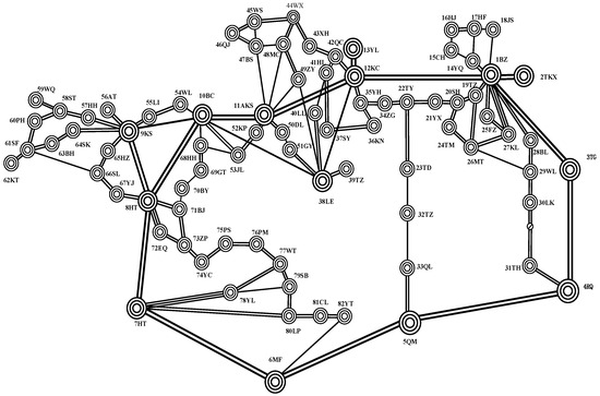
Figure 3.
Topology Diagram of the Regional Main Grid.
5.2. System Partition and Frequency Measurement Point Selection
According to the flowchart shown in Figure 1, the edge weights of the power system graph are set as the reciprocal of the electrical transmission line impedance values, thereby constructing an adjacency matrix W to represent the intrinsic connection strength between any two nodes in the system. The spectral clustering algorithm is then applied to cluster all nodes in the power system. When the system is divided into four zones, the CH index reaches its maximum value on the CH curve. The corresponding partitioning result is presented in Figure 4.
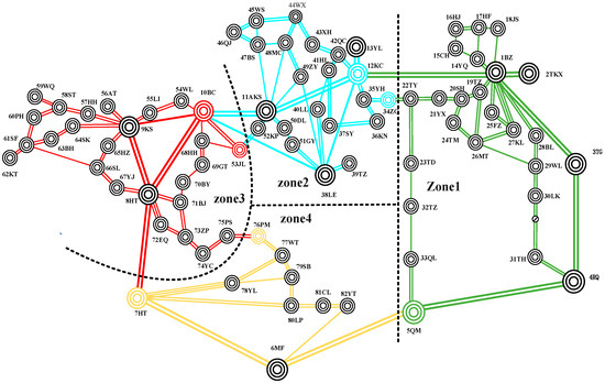
Figure 4.
Partition Topology Diagram.
Due to factors such as geographical location and topographical conditions, different types of generating units are installed in each zone. Table 2 lists the types of generating units and their power generation capacity within each zone. Based on the zoning results in Figure 4, there are eight interconnecting lines between the four zones, requiring the installation of parameter measurement equipment to calculate the power exchange between zones.
Table 2.
Installed Capacity by Partition.
After completing the system regional division via spectral clustering algorithms, the Pearson correlation coefficient matrix was employed to identify the characteristic nodes for each region. Following the methodology described in Section 2.2, the constructed model was subjected to three types of disturbances: generator tripping, load increase/decrease, and N-1 short circuits. A total of 22 disturbance scenarios were configured, with disturbance power ranging from a minimum of 100 MW to a maximum of 2000 MW. To enhance the reliability of node selection, a backup node selection mechanism has been introduced. After regional partitioning, the Pearson correlation coefficients of nodes within each region are calculated and ranked under various operating conditions and disturbance scenarios. The node with the highest correlation coefficient is selected as the primary node, while the node with the next highest coefficient serves as the backup node. When the primary node fails to accurately reflect regional frequency due to extreme disturbances or operational constraints, the backup mechanism is activated, and the backup node assumes responsibility for uploading frequency data. This design ensures that even if primary node selection fails, the backup node can still precisely reflect regional frequency changes. The final primary and backup nodes for each region, along with their corresponding selection probabilities, are summarized in Table 3.
Table 3.
Nodes and Their Selection Probability by Partition.
The results presented in Table 3 indicate that, under a fixed grid topology, different types of disturbances have a limited impact on node selection, which verifies the effectiveness and robustness of the proposed method. Based on these results, nodes BZ, AKS, KS, and HT are selected as the primary nodes for their respective regions, while nodes TG, LE, BC, and MF are designated as the corresponding backup nodes. These nodes are subsequently used to characterize the overall system frequency response of each region.
5.3. Cutting Zone Selection and Feasibility Verification
To validate the effectiveness of the proposed regional selection method for the cutting machine, a permanent N-1 fault occurred on the regional power transmission channel 12KC-13YL at 0.2 s. Figure 5 shows the frequency fluctuation curves at the nodes for each region.
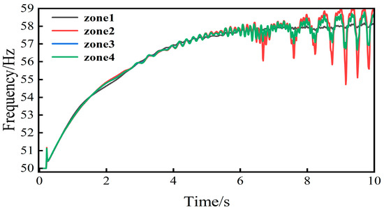
Figure 5.
Frequency Fluctuation Curves of Cmax Nodes in Each.
As shown in Figure 5, when an N-1 short-circuit fault occurs at 0.2 s, the frequency experiences a momentary surge exceeding 51 Hz. The system’s inherent frequency regulation capability rapidly responds to the high-frequency fault by adjusting the frequency. However, the severity of the high-frequency fault exceeds the system’s self-adjustment capacity, causing the frequency to rise too quickly and ultimately surpass the system’s tolerance threshold, leading to system collapse.
When an N-1 short-circuit fault occurs in the system at 0.2 s, the rapid protection device disconnects the permanently faulty line at 0.3 s. The resulting power redundancy from the interrupted power transmission channel prevents high-frequency faults from dissipating, causing the frequency to exceed the normal operating range. Figure 6 shows the frequency fluctuation after fault clearance.
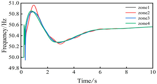
Figure 6.
Frequency Fluctuation Curve After Fault Clearing.
As shown in Figure 6, a brief frequency dip occurs after the 0.3 s fault clearance. However, due to power redundancy, the frequency promptly recovers to approximately 51 Hz. The system’s inherent frequency regulation capability then readjusts the frequency, ultimately stabilizing it around 50.5 Hz. The maximum frequency value at node AKS in Figure 5 exceeds that of the other three nodes, indicating that the fault’s impact on nodes within this region is greater than on nodes in other zones.
To address high-frequency issues following fault clearance, generator tripping operations are performed to achieve power balance. After 0.3 s of fault clearance, the system exhibits a power redundancy of 1495.7 MW. The priority generator tripping zones are selected and validated using the methodology provided in Section 3. Table 4 presents the indicator values, corresponding weights, and composite indicator scores for the four regions. To eliminate interference caused by differing units of measurement among indicators, all indicators were normalized using the range method.
Table 4.
Partition Indicators and Overall Indicator.
As shown in Table 4, the comprehensive indicator indicates that zone 2 has a significantly higher value than other regions. Therefore, zone 2 is selected as the priority zone for generator tripping, followed by zone 1 as the secondary shedding zone, then zone 4, and finally zone 3. Following the selection of unit-dismissal zones, the operation was executed. Ultimately, 860 MW of units were dismissed in zone 2 and 480 MW in zone 1, totaling 1340 MW. The system frequency recovered to 50.05 Hz. The capacity diagram of the generator tripping is shown in Figure 7 The frequency curve is shown in Figure 8, demonstrating compliance with the stable operating frequency range of 49.8 Hz to 50.2 Hz. This confirms the feasibility of the proposed method.
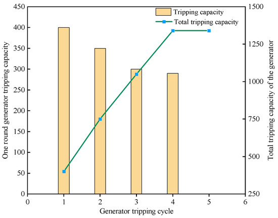
Figure 7.
The capacity diagram of the generator tripping.
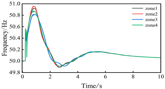
Figure 8.
Generator Tripping Frequency Recovery Curve.
5.4. Comparison of Different Solutions’ Effects
Section 5.1 presents a comprehensive scoring system under the proposed regional classification framework. By weighting regional power surplus ratios, equivalent inertia time constants, frequency deviations, and RoCoF, a composite score is derived. This score determines the sequence for selecting regions for generator tripping operations, arranged in descending order. Section 5.2 presents simulation verification of the proposed method. Results confirm that the method fully meets high-frequency shedding criteria, restoring system frequency to stable operating ranges. This section presents a comparative analysis of the proposed strategy, the grid’s current distributed control strategy, and an advanced centralized generator tripping strategy based on response information. The comparison is conducted by evaluating the maximum frequency, minimum frequency, steady-state frequency, and final amount of generator tripping following the implementation of each control method, leading to the corresponding conclusions.
As shown in Table 5, compared with existing decentralized control strategies for the power grid, the proposed method not only achieves better frequency recovery, but also reduces the generator trip capacity by 6.29%. Compared with advanced centralized strategies, it reduces recovery time by 10% while achieving good frequency recovery.
Table 5.
Frequency Variation and Tripped Generator Capacity under Different Control Strategies.
Figure 9 presents the voltage recovery curves at key nodes under the three control strategies. Compared with both the distributed and centralized control methods, the proposed strategy achieves a smoother recovery trajectory with less overshoot, demonstrating superior voltage support characteristics.
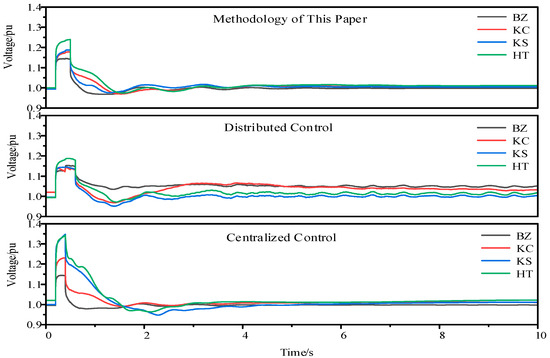
Figure 9.
Comparison of voltage recovery curves.
Figure 10 shows the frequency recovery curves after generator tripping for the proposed method, distributed control, and centralized control, as determined by the node frequency across four regions.
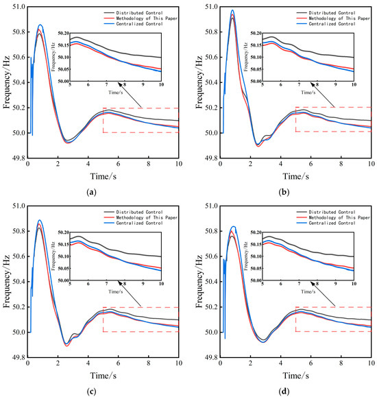
Figure 10.
Comparison Chart of Control Effects. (a) Frequency Comparison of Cmax Nodes in zone 1; (b) Frequency Comparison of Cmax Nodes in zone 2; (c) Frequency Comparison of Cmax Nodes in zone 3; (d) Frequency Comparison of Cmax Nodes in zone 4.
As shown in Figure 10, the proposed method significantly reduces data analysis time by shifting the central controller’s processing focus from raw massive data to key feature data aggregated regionally. Compared to centralized control methods, this approach delivers faster response times while achieving comparable frequency restoration performance. Simultaneously, this approach leverages distributed data acquisition to circumvent the massive data analysis and latency issues inherent in centralized architectures. It further overcomes the lack of coordination between regions in decentralized control through lightweight central intelligent decision-making, achieving global coordinated optimization under rapid response conditions. Although its action time lags slightly behind decentralized control methods, its frequency recovery performance is markedly superior.
6. Conclusions
Existing research on high-frequency generator tripping control predominantly relies on single or limited indicators for decision-making, often employing either centralized architectures with high computational burdens or decentralized schemes lacking global coordination. With the increasing integration of renewable energy, power systems now exhibit characteristics such as low inertia, strong power fluctuations, and spatially heterogeneous frequency dynamics. These developments render traditional control strategies inadequate in meeting the demands for rapid response, adaptability, and system-wide coordination. Consequently, there is a pressing need for generator tripping strategies capable of accurately locating disturbance sources and prioritizing generator tripping zones in real-time. To address these challenges, this study proposes a novel partition-based cooperative decision-making framework for high-frequency generator tripping. The main contributions are as follows:
- (1)
- Dynamic Zoning and Representative-Node Sensing Mechanism: A dynamic partitioning method integrating spectral clustering with Pearson correlation analysis is developed to adaptively divide the power system into electrically coherent zones. Each zone is represented by a characteristic monitoring node, which accurately captures regional frequency dynamics. This approach significantly reduces data transmission volume and central processing load.
- (2)
- Two-Layer Lightweight Cooperative Control Architecture: A hierarchical control architecture comprising “zone controllers + a central controller” is designed. Zone controllers are responsible for fast local sensing and data aggregation, while the central controller performs lightweight global optimization to generate coordinated generator tripping sequences. This architecture effectively balances responsiveness with global coordination, thereby overcoming the latency inherent in fully centralized control and the incoherence of purely decentralized schemes.
- (3)
- Multi-Indicator Integrated Prioritization Model: A comprehensive four-dimensional evaluation system is established, incorporating the regional power surplus ratio, equivalent inertia time constant, frequency deviation, and RoCoF. Utilizing an AHP with data-driven weight assignment, the model dynamically prioritizes generator tripping zones. This methodology effectively mitigates both over-tripping and under-tripping, particularly in scenarios characterized by low inertia and high penetration of renewable energy sources.
While the simulation results validate the effectiveness of the proposed strategy, several practical implementation challenges need to be considered for future real-world applications.
- (1)
- In practical implementations, the proposed coordinated generator tripping framework relies on communication among regional controllers and the central decision layer. Although limited information exchange is required, cybersecurity issues such as data integrity, communication reliability, and malicious attacks deserve further investigation. Future research will focus on integrating secure communication protocols, intrusion detection mechanisms, and cyber-resilient control strategies to enhance the robustness and practical applicability of the proposed method.
- (2)
- The current validation is primarily focused on a single typical regional power grid and specific fault scenarios. The generalizability of the proposed strategy under broader grid topologies, higher gradients of renewable energy penetration, and compound fault conditions requires further investigation. Future work will involve multi-scenario testing across various renewable energy penetration levels to verify the robustness and widespread applicability of the proposed strategy.
Author Contributions
Conceptualization, W.S. and H.W.; methodology, W.S.; software, W.S. and H.W.; validation, W.S., Z.L. and H.Z.; formal analysis, W.S. and H.W.; investigation, W.S., H.W. and X.W.; resources, H.W.; data curation, W.S.; writing—original draft preparation, W.S.; writing—review and editing, H.W.; visualization, W.S.; supervision, Z.L.; project administration, W.S. and X.W.; funding acquisition, H.W. All authors have read and agreed to the published version of the manuscript.
Funding
This research was funded by Science and Technology Project of State Grid Corporation of China, Research on the High-Frequency Switching Control Technology and Applications Considering Disturbance Resistance and New Energy Participation (Grant No. 5100-202440016A-1-1-ZN).
Data Availability Statement
The original contributions presented in this study are included in the article. Further inquiries can be directed to the corresponding author.
Conflicts of Interest
Authors Zhaowei Li, Hongli Zhang and Xuelian Wu are employed by the State Grid Electric Power Research Institute. The remaining authors declare that the research was conducted in the absence of any commercial or financial relationships that could be considered a potential conflict of interest.
Appendix A
Table A1.
List of Abbreviations.
Table A1.
List of Abbreviations.
| Full Name | Abbreviation |
|---|---|
| Analytic Hierarchy Process | AHP |
| Between-Group Sum of Squares | BGSS |
| Calinski–Harabasz | CH |
| Direct Current | DC |
| Doubly Fed Induction Generator | DFIG |
| Phasor Measurement Unit | PMU |
| Photovoltaic | PV |
| Voltage Source Converter | VSC |
| Rate of Change of Frequency | RoCoF |
| Wide Area Measurement System | WAMS |
| Within-Group Sum of Squares | WGSS |
Table A2.
Main equipment parameters of system.
Table A2.
Main equipment parameters of system.
| Generator Set Type | Parameter Type | Parameter Value |
|---|---|---|
| Doubly Fed Induction Generator | Rated voltage UN | 690 V |
| Rated Power PN | 1.5 MW | |
| Rated Wind Speed Vn | 11 m/s | |
| Cut-in wind speed Vcutin | 3 m/s | |
| Cut-out wind speed Vcutout | 20 m/s | |
| Rotor Radius R | 44.55 m | |
| Generator Moment of Inertia JGEN | 58 kg/m2 | |
| Gearbox Ratio Ngear | 106 | |
| Maximum Power Limit Pmax | 1.0 pu | |
| Minimum Power Limit Pmin | 0.04 pu | |
| Servo Time Constant TP | 0.3 s | |
| Maximum Pitch Angle Limit Dmax | 30° | |
| Minimum Pitch Angle Limit Dmin | 0° | |
| Steam Turbine | Rated voltage UN | 20 kV |
| Governor Droop Coefficient R | 0.05 | |
| Prime Mover Maximum Power Output Pmax | 1.0 pu | |
| Prime Mover Minimum Power Output Pmin | 0.8 pu | |
| Servomotor Time Constant T | 0.1 s | |
| Maximum Valve Opening Rate Vopen | 2 pu/s | |
| Maximum Valve Closing Rate Vclose | 2 pu/s | |
| Hydraulic Turbine | Rated voltage UN | 10.5 kV |
| Governor Droop Coefficient R | 0.04 | |
| Governor Response Time TG | 0.3 s | |
| Pilot Valve Time Constant TP | 0.04 | |
| Transient Droop Time Constant Td | 3 s | |
| Transient Droop Gain Dd | 0.4 | |
| PV Module | Rated voltage UN | 400 V |
| Grid-Connected PV System Topology | Two-Stage | |
| Open-Circuit Voltage of a Solar Cell under STC UOC | 44.8 V | |
| Short-Circuit Current of a Solar Cell under STC Isc | 8.33 A | |
| Maximum Power Point Voltage (Vmp) of a Solar Cell under STC Um | 35.2 V | |
| Maximum Power Point Current (Imp) of a Solar Cell under STC Im | 7.95 A |
References
- You, S.; Liu, Y.; Kou, G. Nonidentification of inertia distribution change in high renewable systems using distribution level PMU. IEEE Trans. Power Syst. 2017, 33, 1110–1112. [Google Scholar] [CrossRef]
- Li, D.; Dong, N.; Yao, Y. Equivalent inertia estimation of a power system containing wind power considering dispersion of frequency response and system partitioning. Power Syst. Prot. Control 2023, 51, 36–45. [Google Scholar] [CrossRef]
- Wang, H.; He, P.; Wen, B. Decentralized Under-frequency Load Shedding Scheme Based on Response Information. Power Syst. Technol. 2019, 43, 2976–2982. [Google Scholar]
- Xu, H.; Ding, Y.; Wang, R. Optimal Allocation of Shared Energy Storage Based on Transmission Network Zoning. Proc. CSEE 2025, 45, 7539–7551. [Google Scholar]
- Chen, J.; Wang, C.; Nan, D. Research on sub/super-synchronous oscillation detecting, alarming and control technology used in the new energy pooling area. Electr. Eng. 2018, 19, 72–76. [Google Scholar]
- You, W.; Zhou, Z.; Chen, L. Study on Mutual Influences between UHVDC and the Receiving-End AC System in Hunan Based on PSASP. Power Syst. Clean Energy 2016, 32, 18–24. [Google Scholar]
- Wang, T.; Liu, J.; Zhu, S. Transient Stability Assessment and Emergency Control Strategy Based on Random Forest in Power System. Power Syst. Technol. 2020, 44, 4694–4701. [Google Scholar]
- Li, Z.; Fang, Y.; Wu, X. Influence of action delay and amount on the control effectiveness of low inertia systems in frequency emergency control. Trans. China Electrotech. Soc. 2024, 39, 5394–5405. [Google Scholar]
- Wang, Z.; Wu, W.; Zhang, B. Fully Distributed Power Dispatch Method for Fast Frequency Recovery and Minimal Generation Cost in Autonomous Microgrids. IEEE Trans. Smart Grid 2016, 7, 19–31. [Google Scholar] [CrossRef]
- Li, Y.; He, Q.; Wang, H. Centralized Control Strategy for Hybrid Microgrid Based on Layered Event Triggering. Electr. Power 2024, 57, 73–82. [Google Scholar]
- Xiao, X.; Zheng, Z. New power systems dominated by renewable energy towards the goal of emission peak & carbon neutrality: Contribution, key techniques, and challenges & carbon neutrality: Contribution, key techniques, and challenges. Adv. Eng. Sci. 2022, 54, 47–59. [Google Scholar]
- Milano, F.; Ortega, A. Frequency divider. IEEE Trans. Power Syst. 2017, 32, 1493–1501. [Google Scholar]
- Barzegar-kalashani, M.; Seyedmahmoudian, M.; Mekhilef, S. Small scale wind turbine control in high speed wind conditions: A review. Sustain. Energy Technol. Assess. 2023, 60, 103577. [Google Scholar] [CrossRef]
- Bastiani, B.A.; Deoliveira, R.V. Adaptive MPPT control applied to virtual synchronous generator to extend the inertial response of type4 wind turbine generators. Sustain. Energy Grids Netw. 2021, 27, 100504. [Google Scholar] [CrossRef]
- Ma, K.; Yang, J.; Liu, P. Relaying-Assisted Communications for Demand Response in Smart Grid: Cost Modeling, Game Strategies, and Algorithms. IEEE J. Sel. Areas Commun. 2019, 38, 48–60. [Google Scholar] [CrossRef]
- Gao, W.; Liu, Y.; Li, Z. Transient Frequency-Voltage Support Strategy for VSC-MTDC Integrated Offshore Wind Farms Based on Perturbation Observer and Funnel Control. IEEE Trans. Sustain. Energy 2025, 16, 1931–1943. [Google Scholar] [CrossRef]
- Zografos, D.; Ghandhari, M.; Eriksson, R. Power system inertia estimation: Utilization of frequency and voltage response after a disturbance. Electr. Power Syst. Res. 2018, 161, 52–60. [Google Scholar] [CrossRef]
- Huang, Y.; Qing, S.; Xu, B. Graph Cut Method for Dynamic Zonal Reserve Allocation in Power Grid with Wind Power Integration. Proc. CSEE 2020, 40, 3765–3775. [Google Scholar]
- Li, J.; Wu, J.; Li, L. Review on Frequency Safety Assessment and Emergency Control of Power System. High Volt. Eng. 2025, 51, 1817–1833. [Google Scholar]
- Li, D.; Zhang, J.; Xu, B. Equivalent Inertia Assessment in Renewable Power System Considering Frequency Distribution Properties. Power Syst. Technol. 2020, 44, 2913–2921. [Google Scholar]
- Zhou, L.; Qu, G.; Liu, W. Methods and Practical Application of Power Supply Area Division for Distribution. Power Syst. Technol. 2016, 40, 242–248. [Google Scholar]
- Li, K.; Zhang, F.; Ding, L. Differentiation Mechanism Analysis and Coordinated Control Methods for Multi-Area Frequency Deviation in Power Grids. Autom. Electr. Power Syst. 2025, 1–18. Available online: https://link.cnki.net/urlid/32.1180.TP.20250826.2305.008 (accessed on 7 January 2026).
- Xu, Z.; Liu, M.; Wang, Y. Fault Set Progression High-Frequency Generator Tripping Optimization Method for HVDC Sending Grid Based on Multi-Dimensional Indicators. Proc. CSUEPSA 2025, 1–10. [Google Scholar] [CrossRef]
- Zhang, Y.; Zhang, J.; Peng, C. Generator Failure Dependent Adaptive Event-Triggered Load Frequency Control in Interconnected Power Systems. Proc. CSEE 2025, 1–13. Available online: https://link.cnki.net/urlid/11.2107.tm.20250821.1752.014 (accessed on 7 January 2026).
- Wen, Y.; Yang, W.; Wang, R. Review and prospect of toward 100% renewable energy power systems. Proc. CSEE 2020, 40, 1843–1856. [Google Scholar]
- Hang, L.; Liu, X.; Gu, X. Review and prospects of frequency security and stability res search in new type power systems. Zhejiang Electr. Power. 2024, 43, 12–26. [Google Scholar]
- Wang, B.; Yang, D.; Cai, G. Review of research on power system inertia related issues in the context of high penetration of renewable power generation. Power Syst. Technol. 2020, 44, 2998–3007. [Google Scholar]
- Sun, J.; Wang, J.; Du, X. Optimization strategy for energy storage configuration in high proportion wind power system considering frequency safety constraints. J. Electr. Power Sci. Technol. 2024, 39, 151–162. [Google Scholar]
- Qiao, Z.; Du, X.; Xue, Q. Review of large-scale wind power participating in system frequency regulation. Electr. Meas. Instrum. 2023, 60, 1–12. [Google Scholar]
- Xu, B.; Peng, Y.; Zhang, L. Research on primary frequency regulation of DFIG based on optimized load shedding and dynamic inertia control. Renew. Energy Resour. 2021, 39, 1217–1223. [Google Scholar]
- Wan, C.; Qin, H.; He, Z. Hierarchical Cluster Control of Large-Scale Distributed PV Inverters for Coordinated Frequency-Voltage Support. Proc. CSEE 2025, 1–15. Available online: https://link.cnki.net/urlid/11.2107.TM.20250911.1548.002 (accessed on 7 January 2026).


Disclaimer/Publisher’s Note: The statements, opinions and data contained in all publications are solely those of the individual author(s) and contributor(s) and not of MDPI and/or the editor(s). MDPI and/or the editor(s) disclaim responsibility for any injury to people or property resulting from any ideas, methods, instructions or products referred to in the content. |
© 2026 by the authors. Licensee MDPI, Basel, Switzerland. This article is an open access article distributed under the terms and conditions of the Creative Commons Attribution (CC BY) license.