Reciprocating Pump Fault Diagnosis Using Enhanced Deep Learning Model with Hybrid Attention Mechanism and Dynamic Temporal Convolutional Networks

Abstract

Fault diagnosis is critical for ensuring the reliability of reciprocating pumps in industrial settings. However, challenges such as strong noise interference and unbalanced conditions of existing methods persist. To address these issues, this paper proposes a novel fusion framework integrating a multiple-branch residual module and a hybrid attention module for reciprocating pump fault diagnosis. The framework introduces a multiple-branch residual module with parallel depth-wise separable convolution, dilated convolution, and direct mapping paths to capture complementary features across different scales. A hybrid attention module is designed to achieve adaptive fusion of channel and spatial attention information while reducing computational overhead through learnable gate mechanisms. Experimental validation on the reciprocating pump dataset demonstrates that the proposed framework outperforms existing methods, achieving an average diagnostic accuracy exceeding 98% even in low signal-to-noise ratio (SNR = −3 dB) environments. This research provides a new perspective for mechanical fault diagnosis, offering significant advantages in diagnostic accuracy, robustness, and industrial applicability.

1. Introduction

As a crucial fluid conveying equipment in industrial production, reciprocating pumps are widely used in important fields such as the petrochemical industry, power energy, and water supply and drainage systems [1,2]. The stability of their operating states is directly related to the safety and efficiency of the entire production process. Therefore, achieving early and accurate diagnosis of reciprocating pump faults is of great practical significance for reducing operation and maintenance costs and avoiding serious accidents [3].

Traditional fault diagnosis methods for reciprocating pumps mainly rely on manual experience analysis and simple signal processing techniques [4,5]. Although these methods have certain effects in specific scenarios, they have inherent defects such as low diagnostic efficiency, being greatly affected by subjective factors, and limited ability to recognize complex fault modes. With the rapid development of sensor technology and data acquisition systems, fault diagnosis methods based on vibration signals have gradually become a research hotspot. Vibration signals contain rich information about the mechanical state. Through in-depth analysis of these signals, the operating state and potential faults of the equipment can be effectively identified.

In recent years, deep learning technology has demonstrated significant advantages in the field of mechanical fault diagnosis, thanks to its powerful ability to automatically extract features [6,7,8,9]. Models such as Convolutional Neural Networks (CNN) [10], Deep Neural Networks (DNN) [11,12], Recurrent Neural Networks (RNN) [13], and Long Short-Term Memory Networks (LSTM) [14] have been widely applied to feature learning and pattern recognition of vibration signals. Yang et al. [15] developed an enhanced intelligent fault diagnosis approach to address the challenges of extracting discriminative features from vibration signals and improving classification accuracy for machine tool ball screw failures. This method integrates optimized variational mode decomposition with symmetrized dot pattern imaging techniques to handle complex fault characteristics. Song et al. [16] developed an optimized CNN-BiLSTM framework for bearing fault diagnosis. The proposed solution integrated convolutional neural networks with a bidirectional long short-term memory architecture to simultaneously extract high-dimensional spatial features and temporal dependencies from vibration data. However, existing deep learning methods still face numerous challenges when handling vibration signals. Firstly, the vibration signals of reciprocating pumps are characterized by non-stationarity, multi-scale properties, and strong noise interference. Single-scale feature extraction methods struggle to capture comprehensive fault information. Secondly, while traditional attention mechanisms enhance important features, they often lead to the loss of key information in the original signal, thus affecting the diagnostic accuracy. In addition, deep network structures are prone to problems such as gradient vanishing or overfitting. Especially in industrial scenarios with small samples and high noise, the generalization ability of the models is severely restricted.

Temporal Convolutional Networks (TCN) have emerged as a powerful deep learning architecture in recent years [17]. They are designed with causal convolutions and dilated structures. This design allows TCN to effectively capture long-term dependencies in time-series data. Due to these advantages, TCN has been increasingly applied in the field of mechanical fault diagnosis. For example, Huang et al. [18] proposed a fault diagnosis method based on an Attention Mechanism Wide-scale Multichannel Temporal Convolutional Network (AWM-TCN). The core innovation of this approach lies in integrating an attention mechanism with the TCN framework, ensuring the model effectively learns the spatiotemporal characteristics of fault signals while enhancing the importance weights of fault-related features. Li et al. [19] developed a novel fault diagnosis approach that combines a time convolutional neural network (TCN) with multiple-branch mixed attention residual networks (MBMAResNet). This method introduced TCN to capture dependencies in long time-series data and optimize the feature distribution of raw data. Despite their advantages, TCN-based fault diagnosis methods still face several challenges in practical applications. First, the standard TCN structure often uses fixed dilation rates. This can limit its ability to adapt to the multi-scale and non-stationary nature of reciprocating pump vibration signals. Second, TCN relies primarily on convolutional operations for feature extraction. This may lead to the loss of important local details in the original signal. Third, in high-noise environments, the deep network layers of TCN can amplify noise components. This reduces the signal-to-noise ratio of the extracted features. Moreover, the training process of TCN typically requires a large amount of labeled data. In industrial scenarios where labeled fault data is scarce, this requirement becomes a significant limitation. These challenges highlight the need for further improvements to TCN-based approaches for reciprocating pump fault diagnosis.

While TCN shows promise in capturing temporal dependencies, its ability to focus on critical features within vibration signals remains limited. To address this issue, attention mechanisms have been widely integrated into deep learning models for mechanical fault diagnosis. Attention mechanisms are designed to enable models to automatically allocate weights to different parts of input data. This allows the models to focus on important feature regions while ignoring irrelevant or noisy components [20]. In recent years, various attention-based approaches have been proposed and applied in the field. For example, Dong et al. [21] proposed a Dynamic Normalization Supervised Contrastive Network (DNSCN) integrated with a multiscale compound attention mechanism for identifying imbalanced gearbox faults. Han et al. [22] proposed a novel anti-noise deep residual multiscale convolutional neural network integrated with an attention mechanism, named Attention-MSCNN, to tackle the challenge of bearing fault detection in strong noise environments. These methods have been shown to improve the performance of fault diagnosis models by effectively highlighting discriminative features. Despite their success, traditional attention mechanisms still face several challenges when applied to reciprocating pump fault diagnosis. First, many attention mechanisms focus solely on either channel or spatial information. They fail to capture the complex interdependencies between these two domains in vibration signals. Second, conventional attention blocks often introduce significant computational overhead. This limits their applicability in real-time monitoring systems with limited computational resources. Third, in high-noise environments, attention mechanisms may inadvertently amplify noise components. This happens when the model incorrectly assigns high weights to noise-related features. Moreover, most attention mechanisms are designed based on global statistical information. They lack the ability to adaptively capture local fine-grained details that are crucial for identifying early-stage faults in reciprocating pumps. These limitations highlight the need for more advanced attention mechanisms that can address the specific characteristics of reciprocating pump vibration signals.

Therefore, to address the limitations of existing TCN and attention mechanism-based methods in reciprocating pump fault diagnosis, this paper proposes a novel fusion framework that integrates a multiple-branch residual module and a hybrid attention module. The proposed framework aims to effectively capture the multi-scale, non-stationary features of reciprocating pump vibration signals while enhancing the model’s robustness to noise and improving feature representation capabilities. The core design of the framework includes a multiple-branch residual module and a dynamic gate coordinate attention module. The multiple-branch residual module employs multiple parallel feature extraction paths. These paths include depth-wise separable convolutions, dilated convolutions, and direct mapping branches. This design enables the model to capture complementary features from different perspectives and scales. The hybrid attention module combines simplified channel attention with lightweight spatial attention. It introduces a learnable gate mechanism to adaptively fuse channel and spatial information, ensuring that the model focuses on critical fault-related features while suppressing noise interference.

The main contributions of this paper are as follows:

• A novel fusion framework based on a multiple-branch residual module and dynamic gate coordinate attention is proposed for reciprocating pump fault diagnosis. This framework effectively addresses the challenges of multi-scale feature extraction and noise robustness in vibration signals.
• The multiple-branch residual module is designed with parallel feature extraction paths. This module enhances the model’s ability to capture complementary features from different dimensions and scales, thereby improving the representation of complex fault patterns.
• The hybrid attention module is introduced to adaptively fuse channel and spatial information. This module enables the model to selectively focus on critical fault features while reducing computational overhead, making it more suitable for real-time monitoring applications.

The remainder of this paper is structured as follows. Section 2 is mainly about the basic theoretical model for fault diagnosis. Section 3 provides a detailed description of the proposed fusion framework, including the multiple-branch residual module and the hybrid attention module. Section 4 presents the experimental setup, including dataset descriptions, evaluation metrics, and implementation details. Section 5 analyzes the experimental results and compares the performance of the proposed method with other State-of-the-Art approaches. Finally, Section 6 concludes the paper and outlines directions for future research.

2. Theoretical Background

2.1. Convolutional Neural Network

CNN generally consists of several parts: convolutional layers, pooling layers, and fully connected layers. These parts are mainly used to reduce the complexity of the model and extract signal features. Figure 1 depicts the overall structure of a CNN architecture, as shown in Figure 1:

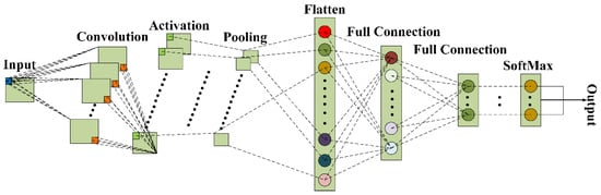
Figure 1. Schematic diagram of CNN framework.

In terms of the temporal characteristics exhibited by the vibration signal, the one-dimensional convolutional neural network (1D CNN) has the ability to extract multi-scale features. It accomplishes this extraction process through the utilization of a local receptive field. The calculation formula of the output is as follows:

$$y=ReLU\left(\sum _{w=1}^W{k}_w{x}_{t-w+1}+b_w\right)$$

(1)

where $k_w$ and $b_w$ are the weight and bias matrix, respectively. $x_{t-w+1}$ are input signals.

The pooling layer is responsible for carrying out feature selection on the input features.

$$y_i=\underset{j\in i}{max} x_j$$

(2)

where $y_i$ is the representation, and j is the neurons in the ith layer.

Activation functions play a crucial role in dealing with the features that are extracted by convolutional layers. After the activation functions have enhanced the feature expressiveness within the CNNs, the subsequent stage focuses on handling the processed features for classification purposes.

2.2. Time Convolutional Network (TCN)

To address the challenges of modeling sequential data in fault diagnosis applications, the Time Convolutional Network (TCN) has emerged as a powerful architecture that offers significant advantages over traditional recurrent neural networks. TCNs excel at capturing long-range dependencies in time series data while maintaining computational efficiency, making them well-suited for analyzing vibration signals from reciprocating pumps.

The fundamental innovation of TCN lies in its use of dilated causal convolutions, which ensure that the network processes data in a strictly temporal order without introducing look-ahead bias. The dilated convolution operation can be mathematically defined as:

$$y\left(t\right)=\sum _{k=0}^{K-1}x\left(t-d\cdot k\right)\cdot w\left(k\right)$$

(3)

where $y\left(t\right)$ represents the output at time $t$, $x\left(t\right)$ denotes the input sequence, $w\left(k\right)$ is the $k$th weight of the convolution kernel, $K$ is the kernel size, and$d$ is the dilation factor. By exponentially increasing the dilation factor with network depth, TCNs achieve a receptive field that expands exponentially while maintaining a linear number of parameters.

For a TCN architecture with multiple layers, the total receptive field $R$ can be calculated as:

$$R=1+\left(K-1\right)\times \sum _{i=0}^{L-1}{d}_i$$

(4)

where $L$ is the number of layers and $d_i$ is the dilation factor of the $i$ th layer. This efficient expansion of the receptive field enables TCNs to capture both short-term transients and long-term periodic patterns in vibration signals, which are crucial for effective fault diagnosis in reciprocating pumps.

2.3. Residual Module

Deep neural networks have demonstrated remarkable performance in various pattern recognition tasks, but training very deep networks remains challenging due to the vanishing gradient problem. To address this issue, He et al. [23] proposed the residual learning framework, which introduces skip connections to facilitate gradient flow during backpropagation. Figure 2 depicts the overall structure of a residual module architecture, as shown in Figure 2:

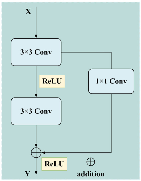
Figure 2. Schematic diagram of the residual module framework.

The residual module consists of a main path and a shortcut connection that bypasses one or more layers. Mathematically, the residual module can be expressed as:

$$x_{l+1}=f\left(x_l+F\left(x_l,W_l\right)\right)$$

(5)

where $x_l$ and $x_{l+1}$ are the input and output of the $l$-th residual block, respectively. $F\left(x_l,W_l\right)$ represents the residual mapping that the network aims to learn. $W_l$ denotes the set of trainable parameters in the block. and $f\left(\cdot \right)$ is the activation function (usually ReLU).

When the input and output dimensions differ, a projection shortcut is employed to match the dimensions:

$$x_{l+1}=f\left(x_l+W_p{x}_l+F\left(x_l,W_l\right)\right)$$

(6)

where $W_p$ is a learnable projection matrix.

2.4. Bidirectional Gated Recurrent Unit (BIGRU)

Bidirectional processing emerged as a critical enhancement to the original GRU architecture. This approach involves handling sequential data by processing it in two separate directions. Specifically, one processing stream operates in the forward temporal direction, moving from the start to the end of the sequence. A second, independent stream processes the data in the backward temporal direction, moving from the end to the start of the sequence. After processing the input sequence in both directions, the hidden states generated by each processing stream are combined through concatenation. This concatenation step produces a comprehensive representation that captures contextual information from both past and future time points relative to each position in the sequence.

As shown in Figure 3, the BiGRU processes an input sequence $X=\left[x_1,x_2,\dots ,x_T\right]$ through two parallel GRU layers. The forward layer computes hidden states by processing the sequence from the first time step to the last, as described by the equation:

$$\overrightarrow{h_t}=GRU\left(x_t,\overrightarrow{h_{t-1}}\right)$$

(7)

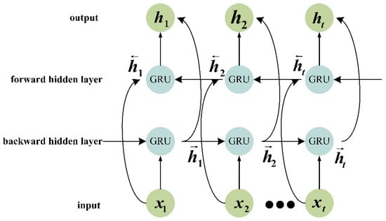
Figure 3. Schematic diagram of the BiGRU framework.

The backward layer computes hidden states by processing the sequence from the last time step to the first, as described by:

$$\overleftarrow{h_t}=GRU\left(x_t,\overleftarrow{h_{t-1}}\right)$$

(8)

The final hidden state at each time step is then derived by combining these forward and backward states through a linear transformation, as follows:

$$h_t=w_t\overrightarrow{h_t}+v_t\overleftarrow{h_t}+b_t$$

(9)

where $\overrightarrow{h_t}$ represents the hidden state at time t in the forward direction, while $\overleftarrow{h_t}$ denotes the hidden state in the backward direction. The parameters, $w_t$, $v_t$, and $b_t$, are learnable weights and biases that determine how the forward and backward states are combined to form the final representation at each time step.

2.5. Reciprocating Pump Signal Segment

As a typical positive displacement fluid machine, the vibration signal of the reciprocating pump has obvious periodicity, non-stationarity, and multi-scale characteristics. Figure 4 shows the time-domain waveforms of the reciprocating pump vibration signals under normal and faulty conditions. It can be observed from the figure that the signal under normal conditions exhibits a stable periodic pattern, and the amplitude range is relatively stable, mainly concentrated between −0.2 and 0.2. Under the fault condition, a relatively high peak appears at the 9000th point, but its shape is different from that under the normal condition, which may indicate a specific fault mode.

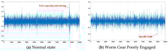
Figure 4. Time-domain vibration signal waveforms of reciprocating pumps under different conditions.

Figure 4 shows the time-domain vibration signal waveforms of the reciprocating pump under normal operating conditions and typical fault conditions. Under normal conditions (Figure 4a), the vibration signal exhibits obvious periodic characteristics, which are consistent with the piston movement frequency of the reciprocating pump. The peaks in the signal (such as the high amplitude at the 8000–9000 points) correspond to the valve opening and closing events, which are the unique operating characteristics of the reciprocating pump. In contrast, the vibration signal under fault conditions (Figure 4b) shows more complex spectral components, the periodic characteristics are weakened, and the high-frequency noise components increase significantly, indicating that there may be mechanical looseness or component wear.

3. Proposed Method

Figure 5 illustrates the architecture of our proposed fusion framework integrating a multiple-branch residual module and a Hybrid Attention module. This framework combines parallel feature extraction paths, adaptive attention mechanisms, and residual connections to enhance fault pattern representation. The input vibration signal first passes through a preliminary convolutional layer for dimensionality reduction and initial feature capture. The multiple-branch residual module then processes these features through three parallel paths: depth-wise separable convolution for efficient local feature extraction, multiple-branch residual module with varying dilation rates to capture multi-scale contextual information, and direct mapping to preserve low-level signal details. Each path operates independently before feature concatenation. The dynamic gate coordinate attention module follows, executing channel-wise and spatial-wise feature recalibration sequentially. Channel attention computes global statistics to prioritize informative frequency components. Spatial attention integrates coordinate information to focus on discriminative spatial regions. A learnable gate mechanism dynamically balances its contributions based on input characteristics. Multiple such module blocks stack to form the deep network backbone. Residual shortcuts connect these blocks to mitigate gradient vanishing and ensure information flow across layers. Finally, feature maps feed into BiGRU and fully connected layers for dimensionality reduction and classification. Softmax activation generates fault category probabilities. Dropout regularization during training prevents overfitting to limited fault samples.

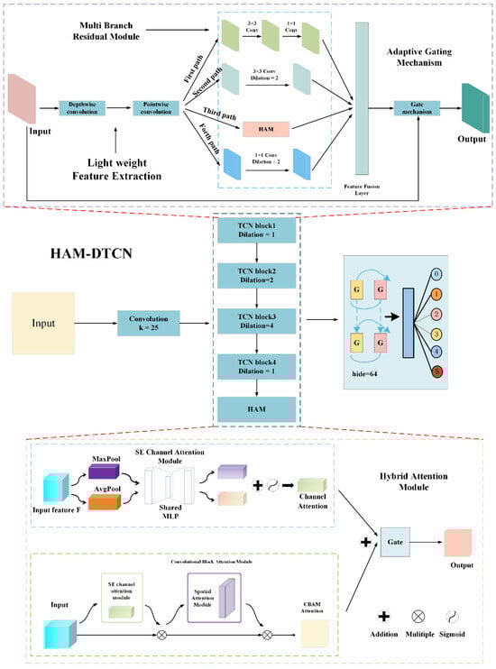
Figure 5. Schematic diagram of the HAM-DTCN framework.

As described in Section 2.5, Branch 1 (dilation rate of 1) of the multi-branch residual module is used to capture high-frequency noise features, corresponding to the irregular vibrations under fault conditions. Branch 2 (dilation rate of 2) is used to capture medium-frequency features, corresponding to the transition process of valve opening and closing events. Branch 3 (dilation rate of 4) is used to capture low-frequency pulsation features, corresponding to the periodicity in the normal state. Meanwhile, the channel attention branch of the hybrid attention module strengthens the key frequency channels, highlighting the valve event features in Figure 4a and the fault features in Figure 4b. The spatial attention branch is used to strengthen the key frequency channels, highlighting the valve event features in Figure 4a and the fault features in Figure 4b.

3.1. Hybrid Attention Module (HAM)

To effectively capture discriminative features from vibration signals with complex patterns and mitigate the information loss caused by over-attention, we propose a novel hybrid attention module (HAM). This module integrates two attention mechanisms: Squeeze-and-Excitation (SE) for channel-wise feature refinement and Convolutional Block Attention Module (CBAM) with a learnable gate to dynamically balance the contributions of attention-enhanced features and original input information.

The HAM, as illustrated in Figure 5, comprises three core components: SE-based channel attention, CBAM-inspired spatial attention, and a learnable gate mechanism. This architecture is designed to leverage the complementary strengths of channel and spatial attention while maintaining computational efficiency, making it particularly suitable for deployment in resource-constrained environments.

3.1.1. SE Channel Attention Branch

SE channel attention branch, as illustrated in Figure 5, is designed to capture interdependencies between feature channels and recalibrate channel-wise feature responses. Given an input feature map $x\in {\mathbb{R}}^{\left(B\times C\times T\right)}$, where B, C, and T respectively represent the batch size, the number of channels, and the sequence length (time steps), we first perform a global average pooling operation to aggregate spatial information across the entire sequence dimension:

$$x_{squeeze}=GAP\left(x\right)$$

(10)

The aggregated features are then reshaped to a 2D tensor and processed through a bottleneck structure to generate channel-wise attention weights. The bottleneck architecture consists of two fully connected layers with a reduction ratio r (set to 32 in this work) to control computational complexity. The number of hidden units in the first fully connected layer is calculated as max (4, C/r) to ensure sufficient representation capacity even for low-dimensional inputs. The channel attention weights are computed as:

$$w_{ch}=\sigma \left(W_2\cdot Swish\left(W_1\cdot x_s\right)\right)$$

(11)

where $x_s\in {\mathbb{R}}^{\left(B\times C\right)}$ is the reshaped version of $x_{squeeze}$, $W_1\in {\mathbb{R}}^{\left(C\times max\left(4,C/r\right)\right)}$ represents the weights of the first fully connected layer, $W_2\in {\mathbb{R}}^{\left(max\left(4,C/r\right)\times C\right)}$ represents the weights of the second fully connected layer, $Swish\left(\cdot \right)$ is the activation function, $\sigma \left(\cdot \right)$ denotes the sigmoid function, and $w_{ch}\in {\mathbb{R}}^{\left(B\times C\right)}$ is the computed channel attention weights.

The resulting attention weights are then reshaped back to match the input dimensions and applied to the input feature map through element-wise multiplication:

$$x_{c{h}_{a}tt}=x\odot w_{ch}$$

(12)

where $x_{ch\_att}\in {\mathbb{R}}^{\left(B\times C\times 1\right)}$ is the reshaped version of $w_{ch}$, and $\odot$ denotes element-wise multiplication.

3.1.2. CBAM

The CBAM branch focuses on capturing discriminative patterns across the time dimension of vibration signals. The framework diagram of CBAM is shown in Figure 6. Unlike the original CBAM, which operates on 2D spatial dimensions, this implementation is tailored for 1D time series data. It first computes the maximum and average values along the channel dimension:

$$x_{max}=max\left(x_{c{h}_{a}tt},dim=1\right)$$

(13)

$$x_{avg}=mean\left(x_{c{h}_{a}tt},dim=1\right)$$

(14)

where $x_{max}\in {\mathbb{R}}^{\left(B\times 1\times T\right)}$ is the maximum value of $x_{ch\_att}$ along the channel dimension, and $x_{avg}\in {\mathbb{R}}^{\left(B\times 1\times T\right)}$ is the average value of $x_{ch\_att}$ along the channel dimension.

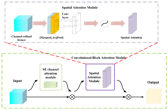
Figure 6. Schematic diagram of the CBAM framework.

These two descriptors are then concatenated to form a feature descriptor containing both intensity and distribution information:

$$x_{cat}=concat\left(x_{max},x_{avg}\right)$$

(15)

where $x_{cat}\in {\mathbb{R}}^{\left(B\times 2\times T\right)}$ is the concatenated feature map.

A 1D convolutional layer with a kernel size of 7 (optimized for capturing temporal dependencies), followed by batch normalization and sigmoid activation, is then applied to generate spatial attention weights:

$$w_{sp}=\sigma \left(BatchNorm\left(Conv1D_{k=7}\left(x_{cat}\right)\right)\right)$$

(16)

where $Conv1D_{k=7}$ denotes a 1D convolutional layer with kernel size 7, BatchNorm is batch normalization, and $w_{sp}\in {\mathbb{R}}^{\left(B\times 1\times T\right)}$ represents the computed spatial attention weights.

The spatial attention weights are then applied to the channel-attended features:

$$x_{s{p}_{att}}=x_{c{h}_{att}}\odot w_{sp}$$

(17)

3.1.3. Learnable Gate Mechanism

A learnable gate mechanism is embedded into HAM to dynamically balance the contributions of the attention-enhanced features and the original input. This gate mechanism is implemented as a scalar parameter initialized to 0.5, allowing the model to adaptively adjust the fusion ratio during training:

$$y=g\times x_{s{p}_{att}}+\left(1-g\right)\times x$$

(18)

where g ∈ [0, 1] represents the learnable gate parameter, and $y\in {\mathbb{R}}^{\left(B\times C\times T\right)}$ is the final output of the HAM. This design ensures that the module preserves critical information from the original input while still benefiting from the attention mechanisms, effectively preventing over-smoothing and information loss.

In summary, HAM effectively captures discriminative features from vibration signals with complex patterns and mitigates the information loss caused by over-attention. By integrating both channel and spatial attention, the module refines features along two orthogonal dimensions, capturing both frequency and temporal discriminative patterns. The learnable gate mechanism dynamically balances attention-enhanced features and original input, preventing over-smoothing and preserving critical information. With an efficient bottleneck design and optimized kernel sizes, the module achieves significant computational savings compared to more complex attention mechanisms.

3.2. Dynamic Temporal Convolutional Block (DTCN Block)

To deal with the problems of multi-scale characteristics and non-stationarity in vibration signals from reciprocating pumps, as well as the trade-off between receptive field and computational efficiency in traditional temporal convolutional networks (TCN), this study proposes a dynamic temporal convolutional block (DTCN block). As shown in Figure 7, the core of this block lies in three key technical schemes: depth-wise separable convolution, multiple-branch residual attention mechanism, and adaptive gating mechanism. These schemes work together to enhance the model’s ability to capture multi-scale features while reducing computational overhead.

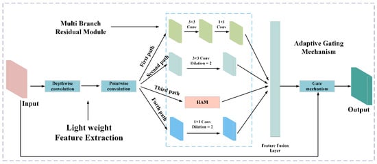
Figure 7. Schematic diagram of the DTCN framework.

3.2.1. Light Weight Feature Extraction

To address the high computational cost of traditional TCN in processing large-scale vibration datasets from reciprocating pumps, DTCN block employs depth-wise separable convolution (DSC) as the fundamental feature extraction unit. DSC decomposes the standard 1D convolution into two sequential operations: depth-wise convolution (DW) and pointwise convolution (PW), effectively reducing the number of parameters while maintaining feature extraction capability. The mathematical formulation of DSC is given by:

$$DW\left(X\right)=\sum _{i=1}^K{X}_i\times K_i$$

(19)

$$PW\left(Y\right)=\sum _{i=1}^K{Y}_i\times W_i$$

(20)

where $X\in R^{C\times L}$ denotes the input feature map with C channels and L sequence length; $K_i$ represents the i-th depth-wise convolution kernel of size $M\times 1$ with a dilation factor; $Y\in R^{C^{\prime }\times L}$ is the output of DW; $W_i$ denotes the i-th pointwise convolution kernel of size 1 × 1; and C′ is the number of output channels. Compared to standard convolution, DSC reduces the parameter count significantly, making it particularly suitable for resource-constrained industrial applications involving reciprocating pumps.

3.2.2. Multiple Branch Residual Module

The multiple-branch residual module’s structural framework originates from rigorous investigation of vibration signal properties in reciprocating pumps. This framework specifically addresses the fundamental multi-scale nature inherent in mechanical vibration patterns. The vibration signals generated during the operation of reciprocating pumps have a complex physical nature, which is specifically manifested in diverse components requiring different receptive field sizes and feature extraction strategies. Traditional single-path convolutional neural networks have obvious limitations in processing such composite features and cannot simultaneously take into account both local transient details and global periodic patterns.

To overcome these drawbacks, this module introduces two key technologies: the multiple-branch parallel architecture and the adaptive feature fusion mechanism. These technologies work together to enhance the model’s capability of capturing multi-scale fault features while maintaining computational efficiency. In terms of specific implementation, the multiple-branch residual module is mainly composed of two parts, namely, multiple-branch feature extraction and adaptive feature fusion. The architecture of multiple-branch feature extraction includes four independent processing paths, each designed to capture different aspects of vibration signals from reciprocating pumps.

Given the input feature map $X\in {\mathbb{R}}^{B\times C\times L}$ (where BC, and L denote batch size, number of input channels, and sequence length, respectively), four paths perform independent operations. The first path employs depth-wise separable convolution to capture local fault features while reducing computational complexity:

$$B_1\left(X\right)=Swish\left(BN\left(Con{v}_{1\times 1}\left(Con{v}_{3\times 3},groups=C(X)\right)\right)\right)$$

(21)

where $\mathrm{C}\mathrm{o}\mathrm{n}{\mathrm{v}}_{3\times 3}$, groups = C represents a depth-wise convolution operation with kernel size 3 × 1 and group count equal to the number of input channels, followed by a pointwise $\mathrm{C}\mathrm{o}\mathrm{n}{\mathrm{v}}_{1\times 1}$ to adjust the channel dimension.

The second path utilizes dilated convolution with a dilation rate of 2 to expand the receptive field without increasing parameters, enabling the capture of longer-range dependencies in signals:

$$B_2\left(X\right)=Swish\left(BN\left(Con{v}_{3\times 3},dilation=2\left(X\right)\right)\right)$$

(22)

where the padding is set to 2 to maintain the output size.

The third path incorporates a HAM mechanism to adaptively enhance important feature channels and spatial locations:

$$B_3\left(X\right)=HAM\left(Con{v}_{1\times 1}\left(X\right)\right)$$

(23)

The fourth path serves as a direct mapping branch to preserve the original information and ensure gradient flow.

$$B_4\left(X\right)=BN\left(Con{v}_{1\times 1}\left(X\right)\right)$$

(24)

where BN denotes batch normalization and Swish represents the activation function.

All four branches are designed to output branch_out = out_channels//4 channels, ensuring balanced feature extraction across different paths and efficient subsequent fusion.

The outputs of the four branches are concatenated into the tensor $F_{cat}$ = [B₁; B₂; B₃; B₄], which contains diverse feature representations from different perspectives. To effectively combine these features, an adaptive fusion mechanism is employed:

$$F_{fused}=\delta \left(BN\left(Con{v}_{1\times 1}\left(F_{c}at\right)\right)\right)$$

(25)

where $\mathrm{C}\mathrm{o}\mathrm{n}{\mathrm{v}}_{1\times 1}$ is used to fuse the concatenated features into the desired output channel dimension, BN denotes batch normalization, and $\delta$ is an activated function that adjusts its shape based on input features.

To address the gradient vanishing problem in deep networks and further enhance feature propagation, a residual connection is introduced:

$$Y=F_{fused}+shortcut\left(X\right)$$

(26)

where shortcut(X) is a projection operation that adjusts the input dimensions through a $\mathrm{C}\mathrm{o}\mathrm{n}{\mathrm{v}}_{1\times 1}$ when the numbers of input and output channels are inconsistent, ensuring the residual connection can be effectively applied.

This multiple-branch residual architecture with adaptive fusion enables the network to capture rich multi-scale features from vibration signals of reciprocating pumps, while maintaining computational efficiency and training stability.

3.2.3. Adaptive Gating Mechanism

To further optimize feature propagation and address the gradient vanishing problem in deep networks, the DTCN block incorporates an adaptive gating mechanism. This mechanism dynamically adjusts the contribution of the main path features and the residual connection, ensuring stable training and effective information flow.

The gating parameter g is a learnable parameter initialized to 0.7, giving higher priority to the processed features initially but able to adapt during training based on the specific characteristics of reciprocating pump vibration signals. The final output of the DTCN block is obtained by a weighted sum:

$$Y=g\times X_{processed}+\left(1-g\right)\times X_{residual}$$

(27)

where $X_{processed}$ represents the features processed through the main path (including depth-wise separable convolution and Multi-Branch Residual attention), and ${\mathrm{X}}_{\mathrm{r}\mathrm{e}\mathrm{s}\mathrm{i}\mathrm{d}\mathrm{u}\mathrm{a}\mathrm{l}}$ is the shortcut connection. This adaptive combination allows the network to dynamically balance between preserving the original information and incorporating the processed features, enhancing the model’s ability to capture complex patterns in vibration signals while maintaining computational efficiency.

4. Results and Discussion

4.1. Data Description

The reciprocating pump dataset, experimental setup, and sensor arrangement used in this experiment are mainly based on our previous research work [24]. This case study applies the proposed method to fault diagnosis in safe injection pumps. The pump model investigated is CDWL25-0.4, which has a rated power of 30 kW. Vibration signals were acquired using an INV3065N2 multi-function dynamic signal testing system together with a piezoelectric accelerometer, model INV982X. A sampling frequency of 10 kHz was set throughout the experiment. Data collection was carried out at Chongqing Water Pump Factory, Chongqing, China [25].

As illustrated in Figure 8, the target of diagnosis is a vertical reciprocating pump. This pump operates through a reciprocating motion along the vertical direction. Six vibration sensors are installed vertically both on the pump head and on the machine foot. The vibration data gathered from these sensors are used to assess the effectiveness and feasibility of the proposed method under cross-sensor domain migration. The labeling of each measurement point is provided in Table 1.

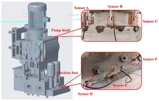
Figure 8. The experimental setup of the reciprocating pump [24].

Table 1. Introduction to measurement points [24].

Sensor Number	Sensor Location	Sensor Number	Sensor Location
A	Vertical direction of pump head 1	D	Vertical direction of machine foot 1
B	Vertical direction of pump head 2	E	Vertical direction of machine foot 2
C	Vertical direction of pump head 3	F	Vertical direction of machine foot 3

The fault samples employed in this investigation originated from natural degradation during operational cycles of the primary coolant injection pump. All failures reflect intrinsic mechanical wear rather than artificial defects. Vibration signals were acquired directly from malfunctioning pump components under real operating conditions. As outlined in Table 2, five fault categories were examined. These include turbine-worm gear misalignment, insufficient bearing lubrication, valve sealing surface fracture, valve sealing surface erosion, and valve sealing surface indentation.

Table 2. Dataset description.

Condition Label	Operating Conditions	Length of Samples
0	Normal state	1024
1	Worm Gear Poorly Engaged	1024
2	Bearing Poor Lubrication	1024
3	Valve Seat Compression Injury	1024
4	Valve Seat Erosion	1024
5	Gearbox Pitting	1024

Vibration data were gathered from predefined measurement points. High-precision accelerometers were used for this purpose. Each raw signal sample has a fixed length of 1024 data points. This length helps capture transient dynamic features effectively. Moreover, these samples are derived from the data collected by pumps of the same model during multiple independent working shifts. Meanwhile, non-overlapping sliding windows (with a window length of 1024 points and a step size of 1024 points) are used to extract samples from the continuous original vibration sequence, ensuring the independence of each sample.

For building the dataset, all vibration sequences belonging to the same operational state were grouped into unified data columns. Each state is associated with a categorical label from 0 to 5. Label 0 corresponds to the normal condition. Labels 1 to 5 represent the five fault types listed in Table 2. This labeling strategy supports supervised learning. It also helps maintain clear distinctions among different mechanical degradation patterns. Moreover, the number of samples for each type is 100. The training set and the test set of the entire dataset are divided in a ratio of 7:3. That is, the total number of samples in the training set is 420, and the total number of samples in the test set is 180.

4.2. Implementation Details

Let α represent the proportion of test samples relative to the total dataset. First, the hyperparameter selection is discussed. Then, the advantages of the newly proposed regularization training methods are evaluated. Performance across different models is assessed as α varies from 0.1 to 0.5, corresponding to approximately 10 to 50 test samples. This evaluation is conducted under a gradually decreasing training set ratio, providing a reference for determining the minimum data requirement in real-world fault diagnosis applications based on deep learning. Finally, model performance is examined under different noise conditions. All experiments are conducted using the same random seed. Detailed experimental configurations are provided in Table 3. In addition, we employed an early stopping mechanism, which uses the validation loss as the monitoring metric. When this metric fails to decrease for 10 consecutive training epochs, the training will automatically terminate. Meanwhile, we adopted a fixed learning rate strategy (Adam optimizer, lr = 0.001). This is because, in preliminary experiments, it was found that, in combination with the early stopping mechanism, a fixed learning rate can already enable the model to converge stably and avoid the additional hyperparameter tuning introduced by learning rate scheduling. To enhance the generalization ability of the model, we used label smoothing regularization (LSR). LSR softens the one-hot encoding of the true labels, thereby reducing the model’s overfitting to the training data. Moreover, we fixed the random seed (seed = 1) to ensure the determinacy and reproducibility of the experiments. To address class imbalance, we employ stratified sampling during dataset division, ensuring proportional representation of each fault category in both training and test sets. And we did not use any speed/rotational speed drift enhancement methods.

Table 3. Description of experimental parameters.

Settings	Value
Batch_size	64
Maximum epochs	100
Optimizer	AdamW
Learning rate	0.001
Weight decay (except bias)	0.0001
Early stopping(patience)	10
AdamW (Nesterov)	Ture

The experiments are implemented using PyTorch 2.1.0 and Python 3.8.7, executed on an AMD Ryzen 7 7840H CPU @ 3.8 GHz with 16 GB RAM. The mini-batch size is set to 8. The ALST framework is employed to supervise the training process of the HAM-DTCN model. To simulate noise interference typical of real industrial environments, Gaussian white noise is added to construct signals with varying signal-to-noise ratios (SNRs). The SNR in decibels is defined as:

$$SN{R}_{\mathrm{d}\mathrm{B}}=10\lg \left({\displaystyle \frac{P_{signal}}{P_{nosie}}}\right)$$

(28)

where $P_{signal}={\displaystyle \frac{1}{N}}\sum _{i=1}^N x_i^2$ denotes the power of the original signal, and $P_{nosie}$ is the power of the noise. Six State-of-the-Art methods are compared with HAM-DTCN: TCN, DRSN [26], WDCNN [27], VACNN [28], and DRCNN [29]. To ensure experimental fairness, the optimizers and loss functions of these six models are replaced with those proposed in this study, thereby validating the effectiveness of the proposed approaches.

The effectiveness of a diagnostic model is commonly evaluated using a confusion matrix, which provides two essential metrics. For multi-class classification tasks, the overall performance is frequently summarized by the macro F1-score. This score represents the harmonic mean of precision and recall, both of which are derived directly from the confusion matrix components as illustrated in Table 4.

$$precision={\displaystyle \frac{TP}{TP+FP}},sensitivity={\displaystyle \frac{TP}{TP+FN}}$$

(29)

$$F_{\beta }={\displaystyle \frac{\left(1+{\beta }^2\right)\left(precision+sensitivity\right)}{{\beta }^2\times precision+sensitivity}}\left(\beta =1\right)$$

(30)

Table 4. Confusion Matrix (TN: True Negative, FN: False Negative, FP: False Negative, TP: True Positive).

		Prediction Category
		True	False
Real Category	True	TN	FP
	False	FN	TP

In these formulations, a true positive (TP) indicates a correct prediction of a positive class instance. A false positive (FP) occurs when the model incorrectly assigns a positive class label. Conversely, a false negative (FN) represents a failure to detect an actual positive instance.

In addition, the label-smoothing training strategy is utilized to supervise the training of the HAM-DTCN model. The structure and main hyperparameters of the HAM-DTCN model are shown in Table 5.

Table 5. Model structure and main hyperparameters of the HAM-DTCN model.

No.	Layer Type	Kernel Number	Kernel Size	Activation	Output Shape
1	Input	-	-	-	(1, 1024)
2	Convolution1	32	25 $\times$ 1	Swish	(32, 512)
3	TCN Block1	64	3 $\times$ 1 (dilation = 1)	Swish	(64, 512)
4	TCN Block2	64	3 $\times$ 1 (dilation = 2)	Swish	(64, 512)
5	TCN Block3	128	3 $\times$ 1 (dilation = 4)	Swish	(128, 512)
6	Max-pooling	-	2 × 1	-	(128, 256)
7	TCN Block4	256	3 $\times$ 1 (dilation = 1)	Swish	(256, 256)
8	Hybrid Attention	-	-	-	(256, 256)
9	BiGRU	-	-	Tanh	(256, 128, 2)
10	AvgPool1d	-	-	-	(256, 1)
11	Flatten	-	-	-	(256)
12	Linear1	64	-	MetaAconC	(64)
13	Dropout	-	-	-	(64)
14	Linear2	6	-	Softmax	(6)

4.3. Robustness Against Noisy Scenarios

In the evaluation of the proposed model’s robustness under varying noise conditions, Gaussian white noise with signal-to-noise ratios (SNRs) spanning from −5 dB to 5 dB was deliberately added to the original vibration signals of the reciprocating pump. All other experimental parameters were kept consistent with the baseline setup. Table 6 presents the detailed performance metrics of the model across different SNR levels, including F1 scores and average accuracy values.

Table 6. Model performance under different SNRs.

SNR	F1 Score	Average Accuracy
−5	0.9386	0.9389
−3	0.9889	0.9889
−1	0.9889	0.9889
1	0.9944	0.9944
3	0.9944	0.9944
5	0.9944	0.9944

As observed from the data, the model achieves an F1 score of 0.9386 and an average accuracy of 0.9389 even at the lowest tested SNR of −5 dB. When the SNR is increased to −3 dB, both the F1 score and average accuracy rise significantly to 0.9889, demonstrating a notable improvement in performance. At an SNR of −1 dB, the model maintains this high level of performance with the same F1 score and average accuracy of 0.9889.

Further increasing the SNR to 1 dB, 3 dB, and 5 dB results in a consistent and optimal performance, with the model achieving the highest recorded F1 score and average accuracy of 0.9944 across all these higher SNR conditions. This trend indicates that the model exhibits remarkable resilience to noise interference, even at very low SNR levels, and maintains stable and high performance as the signal quality improves.

Figure 9 shows the accuracy and loss value curves of the model when SNR = −3. It can be seen from the figure that the loss value curve of the model can still tend to be stable in an extremely strong noise environment, and the accuracy is higher than 95%. Therefore, it can be seen that the model has extremely strong robustness in a noisy environment.

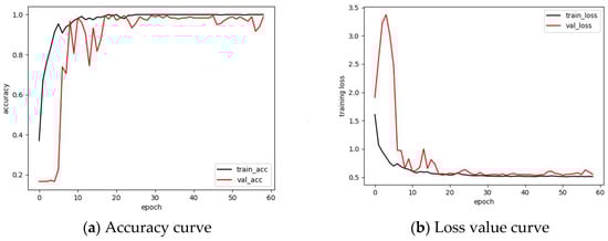
Figure 9. The accuracy and loss value curves of the model when SNR = −3.

To further evaluate the proposed HAM-DTCN model’s performance under noisy conditions, a comparative analysis was conducted with five existing models: DRSN, WDCNN, VACNN, DRCNN, and TCN. As shown in Figure 10 and Table 7, the models were tested on vibration signals corrupted with Gaussian white noise at SNR levels ranging from −5 dB to 5 dB. The performance metrics for all models across different SNRs are presented in the provided data.

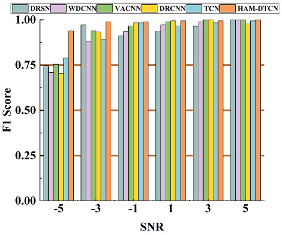
Figure 10. Comparison of six different algorithms under different SNRs.

Table 7. Performance comparison of different algorithms under different SNRs.

SNR	DRSN	WDCNN	VACNN	DRCNN	TCN	HAM-DTCN
−5	0.7468	0.7089	0.7552	0.7039	0.7888	0.9386
−3	0.9721	0.8784	0.9386	0.9333	0.892	0.9889
−1	0.9115	0.9343	0.9667	0.9833	0.9833	0.9889
1	0.9383	0.9723	0.9889	0.9944	0.9663	0.9944
3	0.9654	0.9889	1	1	0.9833	0.9944
5	1	1	1	0.9777	0.9944	1

At the lowest SNR of −5 dB, the HAM-DTCN model achieves an F1 score of 0.9386, which is significantly higher than the next best-performing model, TCN, with 0.7888, while the other models show substantially lower performance at this noise level, with DRSN, WDCNN, VACNN, and DRCNN achieving F1 scores of 0.7468, 0.7089, 0.7552, and 0.7039, respectively, indicating that the HAM-DTCN model exhibits superior noise robustness compared to the other models when the signal quality is very poor; as the SNR increases to −3 dB, the HAM-DTCN model maintains its leading position with an F1 score of 0.9889, while DRSN follows with 0.9721, and at an SNR of −1 dB, the performance of most models improves, but the HAM-DTCN still outperforms all others with an F1 score of 0.988, closely, closely followed by DRCNN and TCN, both at 0.9833; at higher SNR levels of 1 dB and 3 dB, the HAM-DTCN model continues to demonstrate excellent performance, achieving an F1 score of 0.9944, and although some models, such as VACNN and DRCNN, reach perfect scores (1.0000) at these higher SNRs, the HAM-DTCN maintains a consistently high performance across all tested conditions, with the HAM-DTCN achieving a perfect F1 score of 1.0000 at the highest SNR of 5 dB, matching the performance of DRSN, WDCNN, and VACNN.

4.4. Robustness Against Imbalanced Conditions

To investigate the robustness of seven algorithms under imbalanced data conditions, five distinct imbalanced datasets, labeled a, b, c, d, and e, were constructed using the safety injection pump dataset B as the foundation. Detailed information regarding the composition of these five datasets is presented in Table 8. In the experimental setup, each category within the test set contains a consistent 30 samples. However, within the training set, only the normal category is represented by 70 samples. Notably, in dataset e, the number of normal samples exceeds twice the combined number of samples from all faulty categories.

Table 8. Description of the database of five types of unbalanced reciprocating pumps.

Category	Training Samples					Test Samples
	Dataset a	Dataset b	Dataset c	Dataset d	Dataset e
0	70	70	70	70	70	30
1	70	60	50	40	30	30
2	70	60	50	40	30	30
3	70	60	50	40	30	30
4	70	60	50	40	30	30
5	70	60	50	40	30	30

Table 9 and Figure 11 present the comparative analysis of F1 scores among six models across five imbalanced datasets (a to e). The results reveal that the proposed HAM-DTCN model consistently outperforms other State-of-the-Art approaches under varying degrees of data imbalance. Specifically, on dataset a, HAM-DTCN achieves an F1 score of 0.9889, which is significantly higher than the second-ranked DRCNN (0.9662) and demonstrates a notable improvement of 10.86% over the TCN model (0.892). Similarly, on dataset b, HAM-DTCN maintains its superior performance with an F1 score of 0.9889, outperforming DRCNN (0.9333) by 5.96% and TCN (0.8873) by 11.45%. Even on Dataset c, where TCN reaches a relatively high F1 score of 0.9669, HAM-DTCN still exhibits a slight advantage with a score of 0.9778.

Table 9. Comparison of F1 scores of six models under five imbalanced databases.

Models	Dataset a	Dataset b	Dataset c	Dataset d	Dataset e
DRSN	0.8375	0.9157	0.9224	0.4850	0.7675
WDCNN	0.5512	0.5899	0.611	0.6789	0.6364
VACNN	0.8619	0.8385	0.8517	0.8444	0.7331
DRCNN	0.9662	0.9333	0.955	0.8438	0.8163
TCN	0.892	0.8873	0.9669	0.9064	0.7735
HAM-DTCN	0.9889	0.9889	0.9778	0.9833	0.9667

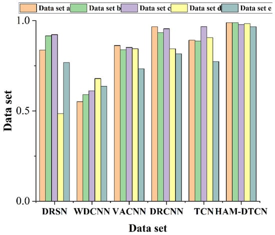
Figure 11. Comparison of F1 scores of six models under five imbalanced databases.

More importantly, the robustness of HAM-DTCN under extreme imbalance conditions is particularly evident in Datasets d and e. On Dataset d, HAM-DTCN achieves an F1 score of 0.9833, which is remarkably higher than DRCNN (0.8438), TCN (0.9064), and VACNN (0.8444), highlighting its ability to effectively handle severe class distribution skews. On Dataset e, which represents the most challenging scenario with the highest imbalance ratio, HAM-DTCN maintains a competitive F1 score of 0.9667, outperforming all other models by a significant margin—for instance, it surpasses DRCNN by 18.42% and TCN by 24.98%.

In the confusion matrix graph, the darker the color, the larger the corresponding number of samples. As shown in Figure 12, the recall rate of HAM-DTCN for each fault category is stably higher than that of the comparison models. Especially in fault category 4, which is the most difficult to identify, the advantage is the most obvious. This fully demonstrates that our model can effectively detect the most critical faults, rather than simply optimizing the overall F1 score. Meanwhile, the success of HAM-DTCN does not come at the expense of rare fault categories. On the contrary, it maintains a high and balanced accuracy rate for all minority classes.

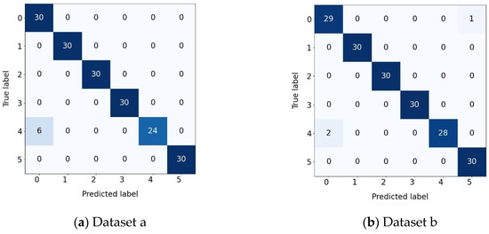
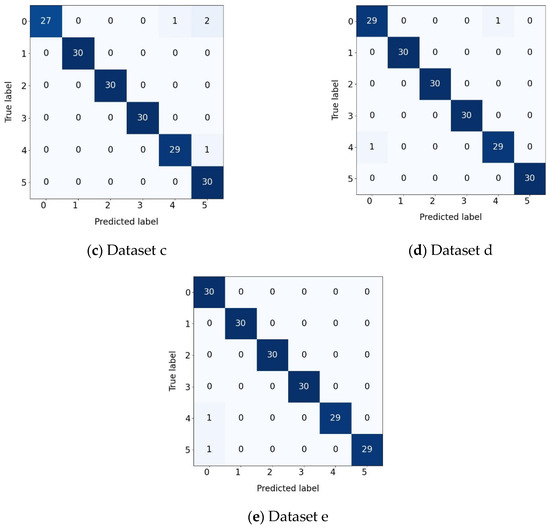
Figure 12. Confusion matrix of different datasets.

5. Ablation Study

In this section, we verify the importance of different modules in HAM-DTCN.

5.1. Effectiveness of the Multiple Branch Residual Module

In this section, we validate the effectiveness of the multiple-branch residual module within the HAM-DTCN model. To conduct ablation experiments, three variant models are designed: HAM-DTCN-RE replaces the multiple-branch residual module with a standard residual block, HAM-DTCN-CNN substitutes it with a simple CNN layer, and HAM-DTCN-SE employs an SE channel attention module instead, while the original HAM-DTCN serves as the baseline model.

In the confusion matrix graph, the darker the color, the larger the corresponding number of samples. As presented in Table 10 and Figure 13, the original HAM-DTCN model achieves the optimal performance with F1 score and average accuracy both reaching 0.9889. In comparison, the HAM-DTCN-RE model yields an F1 score of 0.9167 and an average accuracy of 0.9153, representing a performance decline of approximately 7.22%. The HAM-DTCN-CNN model exhibits a significant performance degradation, with an F1 score of only 0.2636 and an average accuracy of 0.3389. The HAM-DTCN-SE model achieves an F1 score of 0.9507 and an average accuracy of 0.95, which is slightly lower than the original model but superior to the other variants.

Table 10. Diagnostic results of the four models with SNR = −3 dB.

Indicator	HAM-DTCN-RE	HAM-DTCN-CNN	HAM-DTCN-SE	HAM-DTCN
F1 score	0.9167	0.2636	0.9507	0.9889
Ave-Acc	0.9153	0.3389	0.95	0.9889

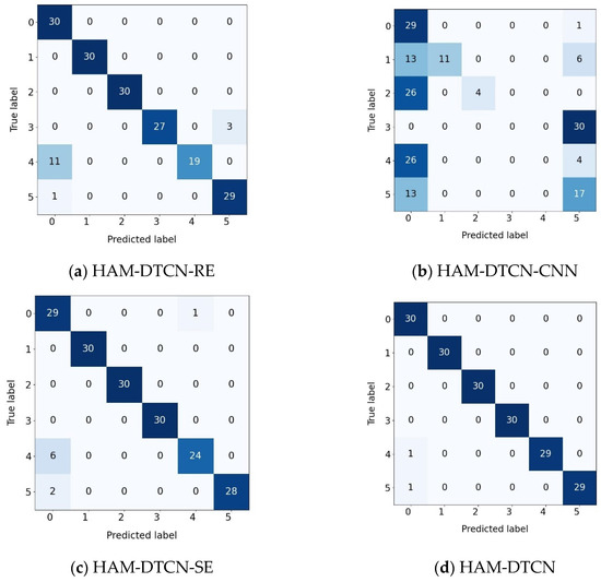
Figure 13. Confusion matrix of different models: (a) HAM-DTCN-RE; (b) HAM-DTCN-CNN; (c) HAM-DTCN-SE; (d) HAM-DTCN.

These results demonstrate that the multiple-branch residual module can effectively enhance the model’s noise robustness through its multi-path feature extraction mechanism. The design of this module, which integrates depth-wise separable convolution, dilated convolution, and lightweight gating mechanisms, enables it to capture complementary features of vibration signals from different dimensions. Particularly in low-SNR environments, the advantages of this multi-path structure become more pronounced, which also explains why the original HAM-DTCN model outperforms the other three variant models.

5.2. Effectiveness of the Hybrid Attention Mechanism (HAM)

In this section, we evaluate the effectiveness of the HAM within the HAM-DTCN model through ablation experiments. Four variant models are designed for comparison: HAM-DTCN-SEA replaces the HAM with an SE channel attention mechanism, HAM-DTCN-CBAM substitutes it with a CBAM attention module, HAM-DTCN-Self employs a self-attention mechanism, and HAM-DTCN-No removes the attention module entirely, while the original HAM-DTCN serves as the baseline. As shown in Figure 14, we employed the t-SNE [30] dimensionality reduction method to project high-dimensional features into a two-dimensional space, facilitating the visual inspection of cluster formations corresponding to different states through color-coding.

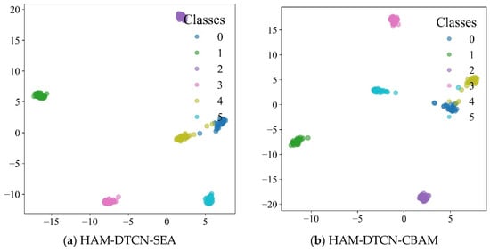
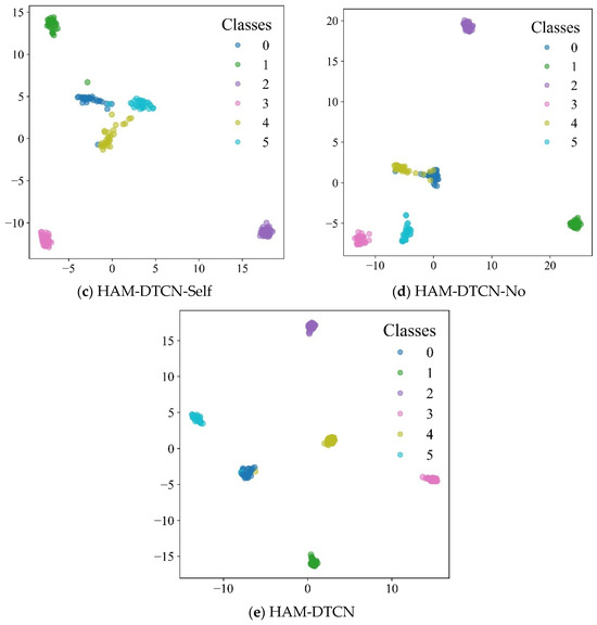
Figure 14. Feature visualization of different models: (a) HAM-DTCN-SEA; (b) HAM-DTCN-CBAM; (c) HAM-DTCN-Self; (d) HAM-DTCN-No; (e) HAM-DTCN.

The experimental results presented in Table 11 demonstrate the superior performance of the original HAM-DTCN model, which achieves the highest F1 score of 0.9889 and average accuracy of 0.9889. Among the variant models, HAM-DTCN-SEA performs the best after the baseline, yielding an F1 score of 0.967 and an average accuracy of 0.9667. The HAM-DTCN-CBAM model follows with an F1 score of 0.9508 and an average accuracy of 0.95. In contrast, the HAM-DTCN-Self model shows a more significant performance decline, achieving an F1 score of 0.8288 and an average accuracy of 0.8222. The HAM-DTCN-No model, which completely removes the attention mechanism, results in an F1 score of 0.8944 and an average accuracy of 0.8969.

Table 11. Diagnostic results of the five models with SNR = −3 dB.

Indicator	HAM-DTCN-SEA	HAM-DTCN-CBAM	HAM-DTCN-Self	HAM-DTCN-No	HAM-DTCN
F1 score	0.967	0.9508	0.8288	0.8944	0.9889
Ave-Acc	0.9667	0.95	0.8222	0.8969	0.9889

These results validate the effectiveness of the HAM in enhancing the model’s feature extraction capability and noise robustness. The module’s unique design, which integrates dynamic gating and coordinate attention mechanisms, enables it to adaptively focus on both channel-wise and spatial information of vibration signals. This multi-dimensional attention approach allows the model to effectively capture discriminative features even in low-SNR environments, outperforming traditional attention mechanisms such as SE, CBAM, and self-attention. The performance gap between HAM-DTCN and HAM-DTCN-No further confirms that the attention mechanism plays a crucial role in improving the model’s diagnostic accuracy and resilience to noise interference.

5.3. Effectiveness of Expansion Rate Schemes

To verify the rationality of the dilation rate scheme design in the Dynamic Temporal Convolutional Block (DTCN Block), the compared schemes include: (a) a [1, 1, 1], where the receptive field remains unchanged; (b) b linearly increasing dilation [1, 2, 3]; and (c) the exponentially increasing dilation [1, 2, 4] adopted in this study. All comparative experiments were conducted under exactly the same parameter budget and network depth, and evaluated in a noisy environment with a signal-to-noise ratio of −3 dB to ensure the fairness of the comparison.

The final experimental performance metrics (average accuracy and F1 score) are summarized in Table 12. The data shows that Scheme (a) achieved competitive results (average accuracy of 0.9833 and F1 score of 0.9835), indicating that even a basic model with a limited receptive field can achieve good performance on this task. However, the performance of Scheme (b) significantly declined (average accuracy of 0.9222 and F1 score of 0.9190). The linear expansion of its receptive field may not have effectively matched the inherent scale distribution of fault features in the vibration signals. Notably, the exponentially increasing configuration of Scheme (c) achieved the optimal performance, with both the average accuracy and F1 score reaching 0.9889, ranking first among all the schemes.

Table 12. Comparison of model performance under different expansion rate schemes.

Indicator	a	b	c
Ave-acc	0.9833	0.9222	0.9889
F1 score	0.9835	0.9190	0.9889

6. Conclusions

This paper addresses the critical challenges in reciprocating pump fault diagnosis under complex industrial conditions, such as strong noise interference and an unbalanced dataset. To tackle these issues, a novel fusion framework integrating a multiple-branch residual module and a hybrid attention module is proposed. The effectiveness and superiority of the proposed framework are systematically verified through extensive experiments on the reciprocating pump dataset. We believe that the core idea of the proposed HAM-DTCN architecture has general applicability for dealing with rotating machinery and reciprocating machinery with similar vibration characteristics. However, due to the dynamic characteristics of different devices, the performance of directly migrating the model across devices may decline. Therefore, in the future, we will combine transfer learning to expand the generalization ability of the model.

The key findings of this study can be summarized as follows. First, the proposed multiple-branch residual module effectively captures complementary features from different dimensions and scales. By incorporating depth-wise separable convolutions, dilated convolutions, and direct mapping branches, the module enhances the model’s ability to represent complex fault patterns. Experimental results show that the multiple-branch residual structure significantly improves the diagnostic accuracy compared to single-path feature extraction methods, with an average accuracy increase of 7.22% under low signal-to-noise ratio (SNR = −3 dB) conditions.

Second, the hybrid attention module demonstrates superior performance in adaptively fusing channel and spatial information. This module selectively focuses on critical fault-related features while suppressing noise interference, which is crucial for fault diagnosis in high-noise environments. Ablation experiments confirm that the dynamic gate mechanism outperforms traditional attention mechanisms such as SE and CBAM, with the proposed model achieving an F1-score of 0.9889 compared to 0.967 for SE-based and 0.9508 for CBAM-based variants under SNR = −3 dB.

Finally, the comprehensive evaluation under various noise levels and working conditions validates the robustness and generalization capability of the proposed framework. Even in extremely low SNR scenarios (SNR = −6 dB), the model maintains an average diagnostic accuracy above 90%, significantly outperforming State-of-the-Art methods.

Despite the promising results, there are still some limitations and future research directions to explore. First, the current framework focuses on single-sensor data. Future work could investigate multi-sensor fusion techniques to further enhance fault diagnosis accuracy by leveraging complementary information from multiple sensors. Second, while the model shows good performance under limited training samples, transfer learning approaches could be integrated to further improve its adaptability to new working conditions with scarce labeled data. Third, the interpretability of the deep learning model remains an open challenge. Developing visualization and interpretation methods to understand the decision-making process of the proposed framework would enhance its practical acceptance in industrial settings. Fourth, the focus of this study lies in verifying the diagnostic performance and robustness of the proposed architecture. A systematic evaluation of the inference latency and computational resource consumption of the model on embedded hardware platforms has not been conducted yet. This is the crucial next step towards actual industrial deployment. In future work, we plan to conduct detailed performance profiling on specific edge computing devices (such as the NVIDIA Jetson Nano 4 GB) using model optimization tools (such as TensorRT) to determine a feasible detection window (102.4 ms) and refresh rate (50 Hz). And then, the current framework only relies on the vibration signals of a single sensor. Although vibration analysis is very effective in capturing dynamic mechanical faults, integrating multi-sensor data is expected to further improve the diagnostic accuracy and robustness. Physical signals from other modalities, such as acoustic emission signals, temperature signals, and pressure signals, can provide complementary information for the health status of reciprocating pumps. Intelligently fusing these heterogeneous data streams is expected to identify early faults and complex faults that are difficult to detect from a single data source.

In conclusion, this study presents a novel and effective fusion framework for reciprocating pump fault diagnosis. The integration of a multiple-branch residual module and a hybrid attention module provides a new perspective for addressing the challenges of feature extraction and noise robustness in mechanical fault diagnosis. The proposed method not only achieves State-of-the-Art performance in diagnostic accuracy and robustness but also offers practical insights for the development of intelligent fault diagnosis systems in the industrial sector.

References

- Lai, Y.; Li, R.; Ye, Z.; He, Y. A new fault diagnosis method for reciprocating piston pump based on feature fusion of CNN and transformer encoder. Sci. Prog. 2025, 108, 368504251330003. [Google Scholar] [CrossRef]
- Pavlidou, A.; Mughal, M.W.; Ahmad, M.; Heidari, H. Hardware Modelling and Testing of a Rotating Neuron Reservoir. In Proceedings of the 19th Conference on Ph.D Research in Microelectronics and Electronics, (PRIME) Larnaca, Cyprus, 9–12 June 2024. [Google Scholar] [CrossRef]
- Medina, R.; Sanchez, R.-V.; Cabrera, D.; Cerrada, M.; Estupinan, E.; Ao, W.; Vasquez, R.E. Scale-Fractal Detrended Fluctuation Analysis for Fault Diagnosis of a Centrifugal Pump and a Reciprocating Compressor. Sensors 2024, 24, 461. [Google Scholar] [CrossRef]
- Cabrera, D.; Medina, R.; Cerrada, M.; Sanchez, R.-V.; Estupinan, E.; Li, C. Improved Mel Frequency Cepstral Coefficients for Compressors and Pumps Fault Diagnosis with Deep Learning Models. Appl. Sci. 2024, 14, 1710. [Google Scholar] [CrossRef]
- Yin, Y.; Liu, Z.; Qin, Y. A High-Fidelity Symbolization Method for Reciprocating Pump Vibration Monitoring Data. IEEE Sens. J. 2025, 25, 11613–11621. [Google Scholar] [CrossRef]
- Li, D.; Chen, Q.; Wang, H.; Shen, P.; Li, Z.; He, W. Deep learning-based acoustic emission data clustering for crack evaluation of welded joints in field bridges. Autom. Constr. 2024, 165, 105540. [Google Scholar] [CrossRef]
- Liu, D.; Cui, L.; Cheng, W. A review on deep learning in planetary gearbox health state recognition: Methods, applications, and dataset publication. Meas. Sci. Technol. 2024, 35, 012002. [Google Scholar] [CrossRef]
- Lv, J.; Kuang, J.; Yu, Z.; Sun, G.; Liu, J.; Leon, J.I. Diagnosis of PEM Fuel Cell System Based on Electrochemical Impedance Spectroscopy and Deep Learning Method. IEEE Trans. Ind. Electron. 2024, 71, 657–666. [Google Scholar] [CrossRef]
- Tang, Y.; Zhang, C.; Wu, J.; Xie, Y.; Shen, W.; Wu, J. Deep Learning-Based Bearing Fault Diagnosis Using a Trusted Multiscale Quadratic Attention-Embedded Convolutional Neural Network. IEEE Trans. Instrum. Meas. 2024, 73, 3513215. [Google Scholar] [CrossRef]
- Dao, F.; Zeng, Y.; Qian, J. Fault diagnosis of hydro-turbine via the incorporation of bayesian algorithm optimized CNN-LSTM neural network. Energy 2024, 290, 130326. [Google Scholar] [CrossRef]
- Pandey, R.; Uziel, S.; Hutschenreuther, T.; Krug, S. Towards Deploying DNN Models on Edge for Predictive Maintenance Applications. Electronics 2023, 12, 639. [Google Scholar] [CrossRef]
- Bekri, S.; Özmen, D.; Türkmenoğlu, A.; Özmen, A. Application of deep neural network (DNN) for experimental liquid-liquid equilibrium data of water + butyric acid + 5-methyl-2-hexanone ternary systems. Fluid Phase Equilibria. 2021, 544, 113094. [Google Scholar] [CrossRef]
- Chen, Y.; Zhang, R.; Gao, F. Fault diagnosis of industrial process using attention mechanism with 3DCNN-LSTM. Chem. Eng. Sci. 2024, 293, 120059. [Google Scholar] [CrossRef]
- You, K.; Wang, P.; Gu, Y. Toward Efficient and Interpretative Rolling Bearing Fault Diagnosis via Quadratic Neural Network with Bi-LSTM. IEEE Internet Things J. 2024, 11, 23002–23019. [Google Scholar] [CrossRef]
- Yang, F.; Tian, X.; Ma, L.; Shi, X. An optimized variational mode decomposition and symmetrized dot pattern image characteristic information fusion-Based enhanced CNN ball screw vibration intelligent fault diagnosis approach. Measurement 2024, 229, 114382. [Google Scholar] [CrossRef]
- Song, B.; Liu, Y.; Fang, J.; Liu, W.; Zhong, M.; Liu, X. An optimized CNN-BiLSTM network for bearing fault diagnosis under multiple working conditions with limited training samples. Neurocomputing 2024, 574, 127284. [Google Scholar] [CrossRef]
- Ding, L.; Li, Q. Fault diagnosis of rotating machinery using novel self-attention mechanism TCN with soft thresholding method. Meas. Sci. Technol. 2024, 35, 047001. [Google Scholar] [CrossRef]
- Huang, J.; Wu, G.; Liu, X.; Bu, M.; Qiao, W. Fault diagnosis of planetary gearboxes under variable operating conditions based on AWM-TCN. Comput. Electr. Eng. 2024, 119, 109520. [Google Scholar] [CrossRef]
- Li, Y.; Yang, Z.; Zhang, S.; Mao, R.; Ye, L.; Liu, Y. TCN-MBMAResNet: A novel fault diagnosis method for small marine rolling bearings based on time convolutional neural network in tandem with multi-branch residual network. Meas. Sci. Technol. 2025, 36, 026212. [Google Scholar] [CrossRef]
- Lin, L.; Wu, J.; Fu, S.; Zhang, S.; Tong, C.; Zu, L. Channel attention & temporal attention based temporal convolutional network: A dual attention framework for remaining useful life prediction of the aircraft engines. Adv. Eng. Inform. 2024, 60, 102372. [Google Scholar] [CrossRef]
- Dong, Y.; Jiang, H.; Jiang, W.; Xie, L. Dynamic normalization supervised contrastive network with multiscale compound attention mechanism for gearbox imbalanced fault diagnosis. Eng. Appl. Artif. Intell. 2024, 133, 108098. [Google Scholar] [CrossRef]
- Han, S.; Sun, S.; Zhao, Z.; Luan, Z.; Niu, P. Deep Residual Multiscale Convolutional Neural Network with Attention Mechanism for Bearing Fault Diagnosis Under Strong Noise Environment. IEEE Sens. J. 2024, 24, 9073–9081. [Google Scholar] [CrossRef]
- He, K.; Zhang, X.; Ren, S.; Sun, J. Deep Residual Learning for Image Recognition. arXiv 2015, arXiv:1512.03385. [Google Scholar] [CrossRef]
- Wang, C.; Chen, L.; Zhang, Y.; Zhang, L.; Tan, T. A Novel Cross-Sensor Transfer Diagnosis Method with Local Attention Mechanism: Applied in a Reciprocating Pump. Sensors 2023, 23, 7432. [Google Scholar] [CrossRef] [PubMed]
- Xu, Y.; Zhang, L.; Chen, L.; Tan, T.; Wang, X.; Xiao, H. Attention-Guided Residual Spatiotemporal Network with Label Regularization for Fault Diagnosis with Small Samples. Sensors 2025, 25, 4772. [Google Scholar] [CrossRef]
- Zhao, M.; Zhong, S.; Fu, X.; Tang, B.; Pecht, M. Deep Residual Shrinkage Networks for Fault Diagnosis. IEEE Trans. Ind. Inform. 2020, 16, 4681–4690. [Google Scholar] [CrossRef]
- Zhang, W.; Peng, G.; Li, C.; Chen, Y.; Zhang, Z. A New Deep Learning Model for Fault Diagnosis with Good Anti-Noise and Domain Adaptation Ability on Raw Vibration Signals. Sensors 2017, 17, 425. [Google Scholar] [CrossRef]
- Wang, X.; Mao, D.; Li, X. Bearing fault diagnosis based on vibro-acoustic data fusion and 1D-CNN network. Measurement 2021, 173, 108518. [Google Scholar] [CrossRef]
- Zhang, W.; Li, X.; Ding, Q. Deep residual learning-based fault diagnosis method for rotating machinery. ISA Trans. 2019, 95, 295–305. [Google Scholar] [CrossRef]
- Cieslak, M.C.; Castelfranco, A.M.; Roncalli, V.; Lenz, P.H.; Hartline, D.K. t-Distributed Stochastic Neighbor Embedding (t-SNE): A tool for eco-physiological transcriptomic analysis. Mar. Genom. 2020, 51, 100723. [Google Scholar] [CrossRef]
Disclaimer/Publisher’s Note: The statements, opinions and data contained in all publications are solely those of the individual author(s) and contributor(s) and not of MDPI and/or the editor(s). MDPI and/or the editor(s) disclaim responsibility for any injury to people or property resulting from any ideas, methods, instructions or products referred to in the content. |
© 2025 by the authors. Licensee MDPI, Basel, Switzerland. This article is an open access article distributed under the terms and conditions of the Creative Commons Attribution (CC BY) license (https://creativecommons.org/licenses/by/4.0/).