


Abstract
Tax evasion is a dynamic process reflecting continuous interaction between taxpayers and regulatory institutions rather than a static deviation from fiscal equilibrium. This study introduces a predator-prey model of tax evasion that translates the Lotka-Volterra framework from biology into budgetary dynamics. The model captures the feedback between the volume of tax evasion and the intensity of regulation, incorporating nonlinearity, implicit reactive lag, and adaptive response. Theoretical derivation and numerical simulation identify three dynamic regimes—stable equilibrium, limit-cycle oscillation, and instability—that arise through a Hopf bifurcation. Bifurcation maps in the (r, a), (r, b), and (r, c) parameter spaces reveal how control efficiency, institutional inertia, and behavioral feedback jointly determine fiscal stability. Results show that excessive enforcement may destabilize the system by inducing regulatory fatigue, while weak control enables exponential growth in evasion. The model provides a dynamic analytical tool for evaluating fiscal policy efficiency and identifying stability thresholds. Its findings suggest that adaptive, feedback-based regulation is essential for maintaining long-term tax discipline. The study contributes to closing the research gap by providing a unified dynamic framework linking micro-behavioral decision-making with macro-fiscal stability, offering a foundation for future empirical calibration and behavioral extensions of fiscal systems.
Keywords:
tax evasion; predator-prey model; fiscal dynamics; Hopf bifurcation; regulatory efficiency; nonlinear systems; economic stability MSC:
68U05; 68U20; 93A30
1. Introduction
Tax evasion is a persistent and complex phenomenon that significantly undermines public finance stability, fiscal equilibrium, and the legitimacy of the tax system. In modern economies, it does not manifest solely as individual decisions of taxpayers or firms but as the outcome of a broader network of interactions among taxpayers, control institutions, the state, and the social environment. This phenomenon must therefore be understood as a dynamic system of mutual interactions in which each component continuously responds to changes in others.
Traditional approaches to the analysis of tax evasion, such as the model of Allingham and Sandmo [1] and its later behavioral extensions, assume individual rational decision-making under given probabilities of audit and penalty. Although these models provide a valuable foundation for explaining microeconomic motivations, they are insufficient to capture the macrodynamic interdependencies and regulatory feedback between taxpayers and the state. The real tax system is characterized by nonlinearity, time delays, feedback mechanisms, and adaptive behavior—features typical of complex nonlinear systems analyzed within the framework of dynamical systems theory.
In this context, there emerges a space for interdisciplinary modeling that enables the transfer of insights from physics, biology, and complex systems theory into economics and public finance. The analogy with ecological predator–prey models by Lotka-Volterra [2] provides an intuitive, mathematically tractable representation of the interaction between tax evasion, as prey, and regulatory mechanisms, as the predator. When the state’s regulatory activity intensifies, the volume of tax evasion tends to decrease, thereby reducing the need for enforcement. Conversely, when oversight weakens, evasion begins to grow again. This feedback process generates oscillations or cyclical dynamics that can be formally described using Lotka-Volterra [2] differential equations.
Transferring the principle of ecological equilibrium into the fiscal domain enables capturing equilibrium states, instabilities, and bifurcation transitions in system behavior. The predator-prey model thus provides a framework for analyzing the conditions under which the tax system remains stable, enters cyclical fluctuations, or approaches collapse, the loss of regulatory control, and the exponential growth of evasion. From a fiscal policy perspective, this approach is particularly valuable because it allows identification of the system’s critical parameters (e.g., audit intensity, sanction effectiveness, and taxpayer adaptability) that determine the long-term dynamics of tax discipline.
The purpose of this study is therefore to present the fundamental principle of the predator–prey model applied to the problem of tax evasion, to derive its theoretical structure, to demonstrate its interpretive potential in an economic-regulatory context, and to illustrate its behavior through a simple numerical simulation. The study has an introductory and conceptual character. However, it aims to highlight the potential of this approach for future research in tax discipline, regulatory efficiency, and the dynamic stability of the fiscal system. The proposed model is first theoretically derived from the original Lotka-Volterra system [2], then adjusted for economic interpretation, and finally demonstrated through an example of the interaction between tax evasion volume and enforcement intensity. The conclusion outlines the model’s implications for fiscal policy and possible extensions, including links with empirical data and behavioral models of taxpayer behavior.
Existing studies also highlight that predator–prey-type regulatory cycles appear in the work of Zaklan, Westerhof, and Stauffer [3], who integrate enforcement dynamics into statistical-physics-inspired models of tax evasion. Similarly, Slemrod and Yitzhaki [4] emphasize the macro-level feedback effects between enforcement and compliance. At the same time, the dynamic-regulatory perspective resonates with the work of Bloomquist [5,6], who develops long-run simulation models of compliance cycles. These contributions provide an empirical and conceptual foundation for understanding endogenous oscillations, but do not formalize them as a tractable dynamical system as the Lotka–Volterra framework allows.
2. Literature Review
Mathematical modeling of tax evasion is a complex field of research that quantitatively analyzes taxpayers and regulatory behavior to understand the mechanisms of tax evasion and its propagation, and to design effective strategies to mitigate it. In this context, agent-based models are often employed to examine the interactions among individual actors and to predict emergent properties of the entire system, such as income distribution [7]. These models simulate dynamic processes in which interactions between pairs of individuals from different income classes and sectors of tax evasion led to changes in wealth distribution and the degree of tax compliance [7]. Such models typically implement behavioral rules of taxpayers and detection mechanisms while exploring how network topologies influence the diffusion of non-compliant behavior [8]. Research also indicates that the introduction of taxation and redistribution, combined with heterogeneous taxpayer behavior, strongly affects the shape and characteristics of the resulting income distribution profile [7]. These models often focus on fractions of individuals who exhibit similar tax behavior at a given time, even though their income-class membership may change, allowing a dynamic analysis of the evolution of tax evasion within a population [7].
Simulation approaches frequently employ techniques from artificial intelligence and machine learning, enabling the modeling of informal-economy formation and the testing of policy impacts on its scope and dynamics [9,10]. Some studies even apply variants of the Ising model, initially developed in magnetism theory, in which each “spin” represents a citizen in a compliant or evading state [7]. This approach allows researchers to analyze how changes in tax rates or audit probabilities affect collective behavior and the overall level of tax evasion, while accounting for social interactions and peer-group influence on individual decision-making [11]. Moreover, complex systems composed of a large number of heterogeneous agents, whose macroscopic behavior is not simply the sum of individual characteristics but rather depends on nonlinear interrelations, are increasingly studied in economic contexts [7]. In the field of tax evasion, this implies that individual compliance decisions are shaped not only by economic incentives but also by social norms, perceived fairness, and expectations regarding others’ behavior, producing emergent patterns of compliance at the macro level [12].
Dynamic models with stochastic elements further show that different audit and penalty probabilities can lead to tax evasion and so-called size traps, in which firms avoid growth to escape stricter monitoring [13]. These models highlight that individual personality traits, external narratives, enforcement probabilities, and perceived effectiveness of public goods provision significantly influence the timing and extent of informal economic activity [9]. Findings suggest that adequate public goods provision and robust enforcement mechanisms are complementary; neither is sufficient on its own to curb informal activity effectively [9]. Moreover, perceptions of public good quality, along with income levels and social impacts, significantly influence individual decisions about tax compliance [14].
Furthermore, tax compliance theory emphasizes that individuals’ tax compliance decisions are influenced not only by economic factors but also by psychological and social stimuli, such as perceptions of the fairness of the tax system, ease of compliance, and fears of detection and punishment [15]. This model also incorporates aspects of social influence and norms that can significantly alter individuals’ behavior, leading to tax compliance that goes beyond purely rational economic considerations [16,17,18]. In this context, tax compliance is often understood as a “wicked system,” in which traditional theories such as deterrence, behavioral, and game theories offer only partial insights into complex, interconnected processes [19]. Therefore, it is essential to integrate these diverse perspectives into a coherent mathematical framework that models the nonlinear interactions among economic incentives, social norms, and psychological factors that shape tax compliance decisions [20]. The concept of tax compliance thus shifts from a binary division into fully compliant and non-compliant taxpayers to a behavioral spectrum encompassing varying degrees of compliance [21]. This multidimensional perspective suggests that effective strategies for improving tax compliance must consider not only direct economic incentives and sanctions, but also perceptual and behavioral aspects, such as the perceived likelihood of audit and the amount of fines, that influence taxpayers’ decision-making [22]. Likewise, morality, monetary benefit, deterrence, and authority represent four key factors influencing attitudes toward tax compliance, with morality and deterrence being consistent determinants [22].
While agent-oriented and behavioral models allow for a precise analysis of the microdynamics of taxpayer decision-making and their interactions with the state, macrodynamic approaches based on predator-prey models broaden the view of the systemic behavior of the economy. These models describe mutual adaptation and cyclical oscillations among two or more economic entities, analogous to predator-prey dynamics in an ecosystem, and thus provide a tool for investigating endogenous fluctuations in fiscal stability, innovation, and redistribution processes.
Predator-prey models, initially developed in biomathematics to describe population dynamics, have found wide application in economic theory, where they are used to analyze complex interactions among economic variables [23]. These models allow us to study the oscillatory nature of various economic phenomena and provide a framework for understanding extreme events in a financial context [24,25]. Specifically, in economics, these models are often used to study the dynamics of market shares, innovation cycles, or interactions between legal and illegal firms, in which one group “eats” the resources of the other [26]. This approach allows modeling a scenario where the behavior of one economic entity directly affects the survival and growth of another, for example, in the context of a competitive struggle for resources or customers [26].
A notable application is the Goodwin model, which reworks the Lotka-Volterra framework [2] to illustrate business cycle fluctuations resulting from the conflict between profits and wages, thereby formalizing Marx’s concept of class struggle within capitalism [27]. In particular, the Goodwin model demonstrates that the distributional conflict between capital accumulation (the employment rate) and the wage share can generate endogenous cyclical patterns, leading to persistent oscillations rather than a stable equilibrium [27]. This framework captures the symbiotic relationship among income distribution, labor market forces, and technical change, especially in the context of increasing returns. Such models, which incorporate Kaldor-Verdoorn effects, reveal how sustained productivity growth and constant income shares result from endogenous sources of power, thereby allowing the examination of different economic regimes.
However, the original Goodwin model’s reliance on exogenous technical change and Say’s law limits its ability to fully capture the non-conservative, dissipative nature of socio-economic systems, where endogenous technical progress is a key driver of evolution and increasing returns [27]. As a result, more recent extensions of this basic model have sought to endogenize technological progress and include demand-supply feedback mechanisms, thereby enriching the model’s ability to explain long-term economic dynamics and structural change. Further research has also examined the implications of non-market clearing, supply constraints, and the impact of the quantity level on employment, wages, and consumption, providing a more comprehensive understanding of economic imbalances [28]. This ongoing refinement allows for a deeper analysis of how different degrees of learning regimes and wage sensitivity affect the stability of the monetary system, mimicking both competitive and Fordist accumulation features [27]. In this vein, extending the basic Goodwin model to account for increasing returns and economies of scale via the Kaldor-Verdoorn coefficient provides a more detailed understanding of how labor productivity growth responds to changes in employment rates. Specifically, integrating the learning coefficient, which quantifies the elasticity of labor productivity with respect to economies of scale, with the elasticity of wages with respect to employment provides insights into how transitions from informal to advanced capitalist systems affect overall labor productivity growth. This enriched framework reveals that regimes with low learning rates, characterized by insufficient generation of increasing returns, tend to lock macroeconomic dynamics into an oscillatory trap and exhibit a persistent weakly stable and cyclic loop. Conversely, the high elasticity of productivity growth to economies of scale, characteristic of advanced capitalism, can facilitate the system’s convergence towards a stable trajectory and remove it from oscillatory behavior. This means that government interventions, such as those that stabilize employment amidst wage differentials, become crucial for supporting economic growth and preventing poverty traps, especially in developing economies [29,30]. Furthermore, the interaction between wage rigidity and labor productivity, mediated by the Kaldor-Verdoorn law, significantly affects the oscillatory dynamics of employment and the wage share, thereby propagating feedback into long-term economic growth [27].
This contrast is also supported by existing literature. Classical static deterrence models, most notably those developed by Allingham and Sandmo [1] and later extended by Slemrod [4], explain incentive structures underlying tax behavior but fail to capture dynamic systemic feedback. Agent-based approaches, such as those proposed by Bloomquist [5,6] and Zaklan et al. [3], allow for the simulation of behavioral heterogeneity at the micro level but do not provide analytically tractable conditions for system stability. Goodwin-type macro-dynamic models [29] capture oscillatory economic behavior but are not explicitly designed to analyze interactions between regulation and tax compliance. In contrast, predator–prey economic applications, as discussed by Naimzada and Ricchiuti [31], highlight the suitability of Lotka–Volterra-type structures for modeling endogenous cycles and stability thresholds in socio-economic systems. This approach, therefore, represents a valuable complement to existing models in the analysis of tax evasion dynamics.
Previous research on tax evasion has primarily focused either on the behavioral and microeconomic determinants of tax compliance or on empirical models based on statistical correlations. Although these approaches have yielded valuable insights into individual decision-making and macroeconomic consequences, they lack a unified dynamical framework that captures the interaction between taxpayer behavior and the regulatory system over time. This research gap concerns the absence of a formalized model that simultaneously describes emergent oscillations in tax compliance, regulatory adaptation, and the conditions for fiscal system stability. The study fills this gap by introducing a predator-prey mathematical model that applies the principles of Lotka-Volterra dynamics from biology to budgetary economics. This model allows us to analyze endogenous cycles between the volume of tax evasion and the intensity of control, identify the bifurcation boundaries of fiscal stability, and formalize the relationships among regulatory efficiency, institutional inertia, and behavioral feedback. It thus provides a unified theoretical-dynamical framework that bridges the gap between micro behavioral and macroeconomic approaches to the analysis of tax evasion.
3. Theoretical Foundations of the Model
3.1. Literary Anchoring of Model Parameters
The chosen predator–prey model is conceived as a conceptual dynamical framework, aimed at analyzing qualitative regimes of interaction between tax evasion and regulatory mechanisms, rather than providing exact quantitative predictions of real developments. This approach aligns with the literature that uses dynamical systems to identify stable and oscillatory regimes in socio-economic processes, without the aim of directly predicting specific values [32].
For this reason, the model parameters were not calibrated to a specific national dataset. Still, their meaning, ranges, and interrelationships are anchored in the existing empirical and behavioral literature on tax discipline and fiscal regulation. Such “literature-based grounding” is a common practice in tax compliance and enforcement modelling, especially when the aim is to analyze mechanisms rather than estimate parameters for a specific country [33].
The parameter r, representing the propensity to evade taxes, is closely linked in the literature to the concepts of tax morality, opportunistic behavior, and perceived legitimacy of the tax system. Empirical studies consistently show that willingness to pay taxes depends not only on economic deterrence, but also on social norms, trust in institutions, and perceptions of the fairness of the tax system [33,34]. It has also been shown that taxpayers’ responses to environmental changes can be nonlinear and heterogeneous, with even small institutional changes leading to significant shifts in behavior [35]. In our model, these mechanisms are reflected in the parameter r, which is the internal growth pressure on tax evasion in situations of weakened regulatory action.
The parameters a and c, which capture the effectiveness of control interventions and the transformative effect of successful enforcement, are motivated by extensive empirical research on the effectiveness of tax audits. Experimental and quasi-experimental studies show that increasing the probability of an audit or explicit signals of increased supervision lead to measurable improvements in tax compliance, although with varying degrees of intensity across taxpayer groups [36,37]. Furthermore, detailed analyses of administrative data suggest that the effect of supervision is not only repressive, but also creates feedback loops through improved information and strengthening institutional capacity [38]. In the model, this mechanism is formalized through the interaction terms aNP and cNP, which capture the system’s nonlinear response to regulatory interventions.
The parameter b, representing the natural decay of regulatory capacity, is based on the literature pointing to limitations in public administrative capacity, organizational attrition, and political-budgetary cycles. Research in the area of fiscal capacity of the state documents that the ability to enforce tax rules is conditioned in the long term by available resources, the quality of institutions, and the stability of administration, while their weakening can lead to a decrease in the effectiveness of control even without formal changes in legislation [39]. This phenomenon is captured in the model by the damping term—bP, which represents the gradual decrease in regulatory activity over time. The empirical context for the dynamics of tax evasion and regulation is also the research on tax gaps, especially the value-added tax. The regular reports of the European Commission on the so-called VAT gap document that the extent of tax evasion changes over time and responds to a combination of macroeconomic shocks, administrative capacity, and enforcement policies. These findings support the interpretation of our model as a tool for analyzing stable and oscillatory regimes of the fiscal system. At the same time, the precise quantitative calibration of parameters represents a separate step suitable for the subsequent application phase of the research [40].
Based on the above literature, the model parameters were chosen within economically realistic ranges consistent with empirical knowledge of tax morale, enforcement, and institutional capacity. The aim of this approach is not to reproduce specific time series, but to identify general dynamic mechanisms that are transferable across different fiscal and institutional contexts.
3.2. Assumptions, Simplifications and Limitations of the Model
The literary anchoring of the model parameters in the previous subsection also allows for the explicit formulation of key assumptions and simplifications on which the proposed dynamic framework is based. These assumptions are not understood as a weakness of the model, but rather as a conscious choice that enables an analytically graspable analysis of the basic feedback mechanisms between tax evasion and regulatory activity.
The first significant simplification is the homogenization of state variables. The model works with an aggregated quantity of tax evasion volume N(t) and an aggregated intensity of regulatory activity P(t), thereby abstracting from the heterogeneity of taxpayers in terms of income levels, sector affiliation, compliance costs, or various forms of tax evasion (e.g., income concealment, fictitious costs, carousel fraud). Similarly, regulatory activity is modeled as a single “predatory” force, without an explicit distinction between instruments such as audits, sanctions, incentives, or reputation mechanisms. This aggregation is consistent with the macrodynamic nature of the model and its aim to capture systemic behavior rather than the detailed microstructure of the tax system.
The second important assumption is the consideration of constant parameters r, a, b, c. In reality, the propensity for tax evasion, the effectiveness of control and the regulatory capacity of the state change over time depending on the economic cycle, the political environment, technological progress or social norms. In the presented model, these factors are implicitly incorporated into the parameter values that represent the average or typical regimes of the system’s behavior. This simplification allows for analytical analysis of stability and bifurcation transitions, but limits the model’s ability to capture short-term shocks or regime changes triggered by exogenous events.
A third limitation is the absence of an explicit network or spatial dimension. Social interactions, the diffusion of tax compliance norms, and behavioral imitation play significant roles in reality, as emphasized in agent-oriented and network models of tax evasion. The proposed model captures these mechanisms only indirectly through nonlinear interaction terms that represent the aggregate effect of contacts between taxpayers and regulators.
The above assumptions also indicate natural directions for extending the model in future research. One possibility is to decompose the state variables N(t) and P(t) into multiple subpopulations, for example by income groups, sectors, or types of tax evasion, which would lead to multi-species dynamic systems. Another extension is to introduce time-varying or stochastic parameters that would allow modeling of business cycles, policy changes, or random shocks. Another promising direction is the integration of network structures that would explicitly capture social contagion through tax behavior and heterogeneous interaction patterns.
These possible extensions, however, do not change the fundamental interpretative value of the presented model. On the contrary, they show that a simple predator-prey framework provides a suitable starting point for a systematic analysis of the macrodynamics of tax evasion, which can be gradually extended to more complex models. In this sense, the simplified structure of the model is consistent with its goal—to identify the basic mechanisms of stability, cyclicality and threshold effects in the fiscal system.
3.3. Dynamical Systems and the Basic Principle of Interaction
The predator–prey model belongs to the broader class of second-order dynamical systems that describe the interaction between two mutually dependent entities. In its simplest form, it is an autonomous, nonlinear system of differential equations that defines how the magnitudes of the two populations—the prey N(t) and the predator P(t)—change over time. The first entity, the prey N(t), tends to grow over time according to its intrinsic growth rate, whereas the second entity, the predator P(t), conditions its growth on the existence of the prey. In the absence of prey, the predator population gradually declines. Mathematically, the system is expressed as:
where the functions f and g represent the rate of increase or decrease of a given entity, depending on its current size and on the size of the other entity. In the classical Lotka–Volterra formulation [2], these functions take the following form:
where N(t)—the amount of prey (in our context, the volume of tax evasion over time), P(t)—the amount of predators (the intensity of control and regulatory mechanisms), (r)—the natural growth rate of prey (tax evasion) in an environment without intervention, (a)—the interaction coefficient, which expresses the effect of controls on reducing evasion, (b)—the natural decrease in regulatory activities (e.g., due to costs, resource depletion, political priorities), (c)—the coefficient of transformational efficiency, i.e., how successful interventions strengthen the regulatory apparatus (resource acquisition, reputation effect, higher trust). These Equations (2) and (3) create a feedback system—if the intensity of controls increases (increase in parameter (P), the volume of evasion (N) decreases; but when (N) decreases, the “food” for the regulatory apparatus also decreases, which leads to a weakening of control activity. This creates a typical nonlinear oscillation that can proceed stably or enter a chaotic state depending on the system’s parameters. This system describes a situation where (i) the prey grows exponentially with a rate (r) as long as there is no regulatory (predatory) pressure on it. The model term (rN) therefore represents the “internal growth potential of the system”—in our economic context, this is the natural tendency towards tax evasion in the absence of control or social pressure; (ii) The interaction term (−aNP) means that the presence of the predator dampens the growth of the prey. The product (NP) represents the frequency of clashes between tax subjects and control authorities. The coefficient (a) expresses the effectiveness of control—i.e., to what extent can one “contact” (e.g., control, audit, sanction) reduce the volume of evasion; (iii) In the predator equation, the term (−bP) represents natural decline, in ecology mortality, in the economic environment a decline in regulatory activity, for example due to budgetary constraints, political reluctance, system fatigue or a reduction in the number of inspectors; (iv) The term (cNP) represents a positive feedback loop—if regulators successfully detect leaks, their funding, public trust and resources for further action improve. The coefficient (c), therefore, expresses the efficiency with which success is converted into regulatory capacity.
In an ecological interpretation, one could say that (r) determines “prey fecundity,” (a) “hunting success,” (b) “predator mortality,” and (c) “prey energetic return”. In an economic analogy, these terms take on the meanings of economic activity, regulatory intensity, cost-effectiveness, and institutional feedback effectiveness. The system is nonlinear because changes in (N) and (P) depend on their product (NP). This nonlinearity is crucial: the system’s response is not proportional; a slight change in the intensity of the controls can have a significant impact when the level of escapement is high, and vice versa.
3.4. Equilibrium and Cyclical Behavior of the System
To obtain a basic picture of the dynamics of the system, it is appropriate to determine the equilibrium points (values at which the system “stabilizes”), i.e., such values (N*) and (P*) for which the following holds:
If we apply condition (4) to relation (2):
This means that the equilibrium level of controls (P*) is directly proportional to the natural rate of growth of leakage (r) and inversely proportional to the effectiveness of control (a). If the company is more prone to leakage (higher (r)), a stable system requires a higher intensity of controls; if controls are more effective (higher (a)), a lower level of regulatory pressure is sufficient.
If we apply the same procedure to relation (3):
This result says that the equilibrium leakage level N* depends on the degree of “system fatigue” (b) and on the efficiency of converting successful interventions into institutional capacity (c). If the regulatory system is rapidly “weakening” (large b) or is inefficient (low c), the equilibrium leakage level will be higher.
Points earned:
represents the dynamic equilibrium of the system, a state in which tax evasion and regulatory activity exist in a stable cycle without further trends of growth or decline. However, if any of the parameters exceed a critical value (e.g., a sharp increase (r) or a decrease in the value of parameter (a)), the equilibrium is disturbed, and the system begins to exhibit cyclical fluctuations. The stability of this point, therefore, depends on the parameters (a), (b), (c), (r), and on the type of disturbances that affect the system. A mathematical analysis of the linearization of the system around the equilibrium shows that it is a center, i.e., that it has closed trajectories around the point (N*, P*). By linear approximation around the equilibrium, it can be deduced that the system exhibits cyclical behavior with a period:
which means that the greater the regulatory system’s natural “mortality” (b) or its effectiveness (c), the faster the regulatory cycles. In economic terms, intense but short-term sustained pressure creates fast but shallow cycles, while weaker but sustained pressure leads to slower, more pronounced waves of tax behavior.
3.5. Transferring the Model to the Economic-Regulatory Environment
If we transfer the above relationships to the economic system of tax evasion, then, analogously to the ecological environment, we can interpret the individual members of models (2) and (3) as follows (Table 1):
Table 1.
Economic-biological analogy of predator-prey model parameters.
Together, these parameters create an economic ecology, a model in which fiscal and institutional processes behave analogously to biological populations. However, in real conditions, the financial system is not unlimited—there are limits, saturation points, and thresholds. This means that, unlike a biological system, the monetary system is subject to institutional and behavioral modifications. Therefore, it is appropriate to extend the model to include the logistic growth of prey and the saturation of the regulatory apparatus:
This means that tax evasion cannot grow indefinitely; its growth is slowed by social resistance, legislative barriers, or the system’s economic capacity. The parameter (K) represents the carrying capacity of evasion, the maximum volume that is still realistically achievable. The new term in relation (11), namely (−dP2), represents diminishing returns in regulation; if control activity exceeds a certain level, the benefit of further controls decreases quadratically (system overload, duplication, cost growth).
The system thus extended is closer to real empirical situations, where excessive regulation can paradoxically reduce efficiency, and where tax evasion reaches a natural saturation due to social or technological limitations. This extended model allows for analyzing the system’s stability under more realistic conditions. If regulatory pressure is too low (P slight), the system tends to exhibit exponential increases in evasion. Conversely, if the control activity is exceptionally high (P large), efficiency decreases due to oversaturation and diminishing marginal returns from control. The equilibrium is located between these two extremes, and its nature depends on the elasticity of the parameters (r), (a), (b), (c), (d), (K).
The dynamics of this system are vibrant. Depending on the parameters, the system can be in one of three types of regimes:
- (1)
- Stable regime—damped equilibrium. If the parameters are set so that the regula-tory apparatus can respond flexibly to changes in leakage volume, the oscillation amplitude decreases and the system moves towards a stable state. This corre-sponds to a situation in which a dynamic consensus has been reached between taxpayers and regulators: the rules are sufficiently predictable, sanctions are effective, and the incentive to leak is low. Mathematically, this is a state where all eigenvalues of the Jacobi matrix have negative genuine parts.
- (2)
- Cyclic regime—limit oscillations. Here, the system oscillates around an equilib-rium point with a stable amplitude. Economically, this corresponds to recurring phases: increased control activity → reduced leakage → weakened supervision → increased leakage → increased controls. Such cycles are often observed in practice (e.g., periodic tightening and loosening of fiscal policy). Mathematically, this is a limit cycle, frequently arising through a Hopf bifurcation.
- (3)
- Unstable or chaotic regime. At extreme parameters (e.g., very high (r), low (a), or significant response delays), the system loses periodicity and enters nonlinear chaos. The volume of leakage and the intensity of controls fluctuate irregularly, often with lags that resemble “fiscal crises”—periods of sharp declines in confi-dence and the effectiveness of regulatory instruments. This state is essential from the perspective of regulatory policy: it shows that excessive or insufficient control can have a similarly destabilizing effect.
3.6. Mathematical Analysis of Stability and Bifurcation
3.6.1. Linearization of the System Around the Equilibrium
Every nonlinear dynamical system can be approximated by its linear form around an equilibrium point. If we consider the basic Lotka-Volterra system [2] according to relations (2) and (3) and the equilibrium point according to relation (8), then we can express minor deviations from equilibrium as:
Near equilibrium, the system can be written as:
where J is the Jacobi matrix, which captures the local derivatives of the system with respect to the variables (N) and (P).
3.6.2. Derivation of the Jacobi Matrix
To analyze the local stability of the system, we will use the Jacobi matrix J(N, P) of the dynamical system at the general point (N, P). The Jacobi matrix is defined as:
where:
The partial derivatives of the functions f1 and f2, which form the elements of the Jacobi matrix J(N, P), have the form:
Substituting the equilibrium values into (8), we then obtain:
The relation (17) above represents a pure oscillator matrix: the diagonal elements are zero, indicating the absence of independent damping within individual populations, while the off-diagonal terms represent nonlinear interactions.
3.6.3. Eigenvalues and the Nature of Equilibrium
We obtain the eigenvalues of the system by solving the characteristic equation:
After installation:
Solving Equation (19), we obtain:
The result shows that the system has purely imaginary eigenvalues, i.e., no real component. This means that the equilibrium point is neither stable nor unstable but represents the center—an ideal closed cycle in which N(t) and P(t) change periodically. In the real economic interpretation, this is a cyclical behavior of the tax system: periods of tightening control (growth of P) and subsequent decrease in evasion (decrease of N) alternate at regular intervals. The system thus never “calms down” completely but oscillates in a natural rhythm. If we were to add small damping or stimulating terms to the model (e.g., response delay, random noise, saturation), the eigenvalues would acquire a fundamental component:
where the sign of the real part (α) determines stability:
- if α < 0: the equilibrium is asymptotically stable (damped oscillations),
- if α > 0: the equilibrium is unstable (growing oscillations),
- if α = 0: the system is critically stable (pure cycle).
3.6.4. Extended Model and Jacobi Matrix with Damping
For the extended model with saturation and limitation (10) and (11), the analysis is more complex. First, determine the equilibria. From the first Equation (10):
From the second factor:
From the second Equation (11):
If P* > 0, then:
Substituting P* from the first equation into the second, we get the implicit equation for N*:
This expression defines the condition for the existence of equilibrium and depends on the parameters (a), (b), (c), (d), (r), and (K). Each term of relation (26) can be assigned a unique economic-ecological meaning (Table 2).
Table 2.
Economic interpretation of the terms of the regulatory equilibrium equation.
The equilibrium state occurs when the positive feedback (cN*) exactly balances the dissipation of the regulatory forces (−b) and the losses from the saturation of the system .
After determining the equilibrium values of N* and P*, we can obtain the Jacobi matrix:
The form of this matrix (27) allows us to calculate the route and determinant that determines the qualitative type of equilibrium:
The stability conditions are:
If Tr(J*) = 0 and Det(J*) > 0, the system is on the threshold of a Hopf bifurcation.
3.6.5. Hopf Bifurcation—Emergence of Cyclic Dynamics
In predator-prey dynamical systems, the Hopf bifurcation represents a fundamental mechanism for the transition from stable equilibrium to periodic behavior. When the essential part of the complex coupled pair of eigenvalues of the Jacobian changes from hostile to positive values, a closed trajectory, a limit cycle, is formed around the equilibrium point. This phenomenon corresponds to the transition from stationary tax behavior to cyclical waves of evasion and regulation.
Let us consider the basic model described by relations (10) and (11), where N(t) denotes the volume of tax evasion and P(t) the intensity of regulatory effort. The equilibrium point (N*, P*) for N* > 0, P* > 0 is given by the relations:
The linear approximation around this equilibrium has the form:
where J* is the Jacobian (27). The characteristic equation of the system can be defined as:
where T = Tr(J*) is the trace and Δ = det(J*) is the determinant. A Hopf bifurcation occurs when:
where µ is a bifurcation parameter (e.g., r, c, a, d, K). The first condition means that the fundamental part of the complex conjugate eigenvalues λ1,2 (µ) passes through zero. The second guarantees that the eigenvalues are purely imaginary at µ = µc, i.e.:
while
The third condition, the so-called transversality, ensures that the crossing of the imaginary axis is not tangential but transverse, thereby eliminating the degeneration of higher-order bifurcations. As a result, the equilibrium’s stability changes, and the system exhibits a local limit cycle.
Figure 1 shows the classification of local equilibrium states of a dynamic system according to the sign and the mutual ratio of the trace and determinant of the Jacobi matrix J.
Figure 1.
Stability map in the plane of the trace T and the determinant Δ.
For positive determinant (Δ > 0) and negative trace values (T < 0), the system is in a stable region—either as a stable node or a stable focus, depending on the magnitude of |T| relative to the . The transition through the vertical line T = 0 represents a Hopf bifurcation, in which the fundamental part of the complex-associated eigenvalues passes through zero, and a limit cycle arises in the system. In the region Δ < 0 (pink part), there is a saddle point, which corresponds to an unstable equilibrium with a loss of self-regulation. From an economic point of view, the map expresses the limits of fiscal stability: the left half (T < 0) corresponds to the damped behavior of the system (effective regulation), the right half (T > 0) represents an increase in instability and the emergence of cyclical fluctuations in tax discipline.
With a slight shift of the parameter µ, this pair intersects the imaginary axis, which causes a change in the stability of the equilibrium point and the emergence (or disappearance) of a periodic solution.
The character of the bifurcation is determined by the sign of the so-called first Lyapunov coefficient l1, which is calculated by transforming the system to standard form near the center:
where r is the amplitude, θ the phase variable, α = Re(λ(µ)) ≈ κ(µ − µc), and β is the nonlinear coefficient determining the type of bifurcation. The coefficient β arises from the system’s nonlinear second- and third-order terms and determines the nature of the emerging cycle. The sign of the coefficient β determines the type of bifurcation. We distinguish two basic kinds of Hopf bifurcation:
- If β < 0, a supercritical Hopf bifurcation occurs, in which a stable limit cycle of small amplitude appears when the threshold µc is exceeded, and the equilibrium becomes unstable. The system smoothly passes into an oscillating regime.
- If β > 0, a subcritical Hopf bifurcation occurs, in which an unstable limit cycle appears when the threshold is approached. At the same time, the stable equilibrium persists only until the moment of a sudden jump to large-amplitude oscillations. This type is characterized by hysteresis and nonlinear collapse of stability.
After substituting the equilibrium values, the trace of the Jacobian can be expressed as:
Each term in Equation (39) can be assigned an economic meaning:
- : Saturation of tax evasion—natural dampening of the growth of evasion,
- : attenuation of regulatory effort—reduces the dynamic reactivity of the system,
- : institutional feedback—a destabilizing element,
- : regulation saturation effect—stabilizing element.
The condition T = 0 represents the point at which the destabilizing effect of feedback (c) is exactly balanced by the damping mechanisms (b, d, K). Increasing the value of parameter (c) or decreasing the value of parameters (b), (d) can shift the system into oscillations—repeated phases of “relaxation and tightening” of tax discipline. Analytically and numerically, it is possible to observe:
- (r, c): higher escape motivation (r) shifts the threshold (c) upwards if saturation (d) is significant,
- (a, r): increasing control efficiency (a) reduces P*, weakens damping, and may bring the system closer to the cyclic region,
- (c, d): larger (d) increases the threshold (c), because saturation regulates the dynamics,
- (b, c): larger (b) damps the system, shifts the Hopf limit to higher (c).
Behind the bifurcation boundary, stable or unstable oscillations N(t) and P(t) arise. In the economic interpretation, this corresponds to cyclical phases:
- Growth of tax evasion, which provokes a reaction from the regulatory apparatus,
- Subsequent tightening of controls, reducing evasion,
- After the relaxation of regulation, a new growth of evasion follows—and the cycle repeats.
The intensity and period of the oscillations depend on ω0 and the model’s nonlinear terms. Politically and economically, the system should move on the stable side of the boundary or in a supercritical, slightly cyclical regime with low amplitude.
4. Model Application and Numerical Simulation
4.1. Objective of Numerical Illustration
This section aims to demonstrate the behavior of the predator-prey model at realistic parameter values that reflect the basic economic-regulatory relationships between the volume of tax evasion and the intensity of tax control. The simulation is illustrative; its task is not to calibrate specific data but to understand the qualitative regimes of the system’s behavior: stable equilibrium, cyclical dynamics, and possible bifurcation instability. This model allows us to observe how tax morality, control capacity, and institutional adaptation interact through nonlinear links.
4.2. Basic Simulation Model
The basic form of the model used for the simulation corresponds to the extended system (10) and (11):
where: N(t)—volume of tax evasion at time t, P(t)—intensity of the control system at time t, r—natural tendency to evasion (e.g., social tolerance, low detection), a—effectiveness of control interaction, b—natural decline in control activity, c—feedback of successful interventions (strengthening of the regulatory apparatus), d—saturation of control effectiveness, K—maximum potential for evasion in the system (economic “carrying capacity”).
4.3. Basic Simulation Parameters Used
For illustration purposes, we will use representative values (Table 3):
Table 3.
Representative values of basic parameters used in the simulation.
The initial conditions are set as N(0) = 30, P(0) = 5, which represents a situation of moderate leakage volume and moderate control intensity at the beginning of the period.
4.4. Numerical Simulation and Dynamic Behavior
To verify the model’s theoretical assumptions, a series of numerical simulations was performed to capture the temporal evolution of the interaction between the volume of tax evasion and the intensity of regulatory mechanisms. The model is based on the structure of an extended predator-prey system, in which the dynamics of both variables—tax evasion N(t) and regulatory activity P(t)—evolve through nonlinear linkages, feedback, and system saturation. Numerical solutions were obtained by the ode45 method in the MATLAB 2025b environment, using the implementation of the extended model defined by Equations (10) and (11): where the parameters (r), (a), (b), (c), (d), (K) represent the growth rate, control efficiency, natural decline of regulation, positive feedback of success, system saturation and maximum evasion capacity. The model captures typical phases of the regulatory cycle, transitions between stable and oscillatory states, and nonlinear dynamical phenomena, including the Hopf bifurcation.
The time evolution of the model shown in Figure 2 exhibits the typical cyclical behavior of a predator-prey system, with the volume of tax evasion N(t) and the intensity of regulation P(t) alternating in a periodic rhythm. It is clear from the graph that the system constantly oscillates around the equilibrium values N* and P*, with a phase shift of approximately π/2 between the two variables. This phenomenon can be divided into three basic phases, which together form the regulatory cycle. The time evolution on a normalized scale is shown in Figure 3.
Figure 2.
Time evolution of the volume of tax evasion N(t) and the intensity of control P(t).
Figure 3.
Normalized time course of the control cycle.
Phase 1—Initial growth and delayed regulatory response: At the beginning of the simulation (t ≈ 0–20), there is a sharp increase in leak volume. This growth is driven by the logistic component , which captures the system’s natural tendency to expand if regulatory forces have not yet intervened. The regulatory system responds with a noticeable delay because its dynamics are mediated by the interaction term (cNP). In Figure 2, this is evident in the first part of the graph, where the curve N(t) rises sharply, while P(t) remains at a low level. Mathematically, this is expressed by a positive value of the derivative:
since the positive term (cNP) exceeds the decrease expressed by the term (bP). In economic terms, this is a phase in which regulatory institutions are just beginning to adapt to the rising rate of leakage.
Phase 2—Peak and Back Damping: During the interval of approximately t ≈ 20–80, the regulatory system is activated and reaches its maximum intensity. In Figure 2, this corresponds to a sharp increase in P(t) that follows the culmination of N(t). The growth of the regulatory apparatus begins to exert a dominant effect on leakage through the term (−aNP), leading to a gradual decrease in N(t). At the same time, in this phase, the regulatory system’s efficiency decreases due to saturation, as reflected by the term (−dP2). This phenomenon can be interpreted as system fatigue: additional effort no longer yields proportional results. The peak of P(t) thus precedes the minimum of N(t), which creates a characteristic phase shift of approximately 90°, typical of all predator-prey models. This shift is clearly observable in Figure 2, where the red curve P(t) reaches its maximum shortly before the blue curve N(t).
Phase 3—Decline and relaxation of the system: After the decrease in leakage, the need for regulatory activity also decreases as the (cNP) term approaches zero. The intensity of regulation P(t) therefore begins to decline, and the system enters the relaxation phase. This decrease also allows leakage to grow again, thus closing the entire cycle. In Figure 2, this phase is evident as a simultaneous decrease in both variables, with the reduction of P(t) lagging that of N(t). The system thus returns to a development phase similar to the initial growth phase, creating a periodic structure for the entire cycle.
In the long term, the system tends to oscillate around the equilibrium state. The amplitude and cycle length depend on the ratio of parameters (a), (c), (d), and (r). With a smaller value of parameter (d) (lower saturation of the control), the oscillations are more pronounced and have a longer duration, while higher values of (d) or lower values of parameter (a) lead to the damping of the cycles and a gradual stabilization around the equilibrium. In terms of time, the amplitude and period of these oscillations can be approximated empirically:
where the relationship determines the phase between the variables:
where is the time shift between the peaks of N(t) and P(t), and Tc is the average period of the cycle. In numerical simulations (Figure 2), this shift is approximately π/2, confirming the classical dynamics of the predator-prey system, in which the maximum of control precedes the minimum of evasion. From an economic perspective, the amplitude of AN can be interpreted as the range of fluctuations in the volume of tax evasion. At the same time, AP represents the range of regulatory institutions’ responses. A high AP/AN ratio indicates a strong but delayed response of the state apparatus. In contrast, a decrease in this ratio suggests slow adaptation or an inability to maintain a stable regulatory rhythm.
While the time courses of N(t) and P(t) shown in Figure 2 and Figure 3 reveal periodic changes, the phase plane provides deeper insight into the mutual dynamics of the two variables. By plotting P(t) as a function of N(t), a curve is obtained in the space of state variables that describes the overall cyclical motion of the system in the (N, P) plane. This picture allows us to interpret not only the periodicity itself but also the dynamics’ stability, amplitude, and rotation direction. Figure 4 shows a typical trajectory of the system in the phase plane. The curve describes a closed loop rotating counterclockwise, which is the classic signature of predator-prey models, in which the growth of the “prey” (tax evasion) precedes the development of the “predator” (regulatory activities).
Figure 4.
Phase trajectory of the system in the (N, P) plane.
In the initial phase of the movement, the trajectory shifts upwards and to the right, which corresponds to the growth of N(t) at a still low level of P(t). Subsequently, as regulatory activity increases, the curve turns to the left—the system enters the phase of leakage damping. After reaching the maximum P(t), the trajectory decreases, expressing the attenuation of regulatory activity and the return of the system to the initial point of the cycle. This closed movement represents a limit cycle—a stable periodic trajectory in the (N, P) space.
Mathematically, the shape of the trajectory can be described implicitly from the system:
From the above relation (43), it follows that in the regions where the interaction terms aNP and cNP dominate, the motion approaches an elliptical shape. For small values of the parameter (d) (low saturation of the system), the loop is narrow and regular, which indicates a stable cycle. On the contrary, for larger values of the parameter (d), the loop expands—the amplitude of the oscillations grows, and the system moves further from equilibrium. Changes in the shape of the trajectory can be understood because of the transition between different dynamical regimes:
- Stable cycle: for lower values of parameter (d) and higher values of parameter (a); the trajectory is smooth, closed, and symmetrical, and the amplitude does not change in time.
- Azabicyclic behavior: for higher values of parameter (d) or lower values of parameter (a), the loop deforms, indicating nonlinear oscillations with a slight change in period.
- Chaotic regime: if parameter (c) exceeds a critical value, an irregular trajectory arises, the system no longer oscillates periodically but exhibits irregular loops and dispersion in the (N, P) plane.
The phase plane, therefore, functions as a geometric visualization of stability. Near the equilibrium point (N*, P*), the trajectory can be interpreted as an orbit whose distance from the center expresses the energy of oscillation. The greater the distance, the more pronounced the cycle and the slower it damps out. From an economic perspective, this plane represents the feedback between the extent of tax evasion and the strength of regulatory intervention. Each point on the trajectory represents an instantaneous combination of economic imbalance and state response. The shape of the loop determines whether the system achieves a stable regulatory rhythm or enters cycles of excessive control and subsequent deregulation.
At a low value of the parameter (a—ineffective intervention), the trajectory has a widened shape, and the cycle lasts longer—the state reacts with a delay. At a higher value of the parameter (a), the loop narrows and closes faster—regulation is more effective and the system reaches dynamic equilibrium.
The phase plane reveals the internal structure of the system’s cyclic dynamics, but to understand global changes in behavior as the parameters are varied, a bifurcation analysis is necessary. This method allows us to determine how the qualitative character of the solutions changes—stability, periodicity, or divergent behavior—depending on changes in the model parameters.
From a formal point of view, bifurcation occurs at the point where the stability of the equilibrium solution changes, that is, where one of the characteristic roots of the Jacobi matrix J passes through the real or imaginary axis. In the case of predator-prey models, the most important is the so-called Hopf bifurcation, where the trace of the matrix equals zero (Tr(J*) = 0) and the determinant remains positive (det(J*) > 0). At this point, the stable equilibrium transitions to a limit cycle, indicating a shift from stationary to oscillatory behavior.
The numerical implementation was carried out by systematically reviewing the parameters (r, a), (r, b), and (r, c), and for each pair of values, the system was integrated over a time horizon of T = 300. Subsequently, based on the variability of the solution, it was determined whether the system:
- (1)
- converges with a stable equilibrium,
- (2)
- oscillates around the equilibrium (limit cycle),
- (3)
- diverges into instability.
Each of these states was assigned to the appropriate category and visualized in a two-dimensional parameter map, known as the bifurcation or stability map. In Figure 5, Figure 6 and Figure 7, these areas are distinguished by color:
Figure 5.
Bifurcation map of the system in space (r, a).
Figure 6.
Bifurcation map of the system in space (r, b).
Figure 7.
Bifurcation map of the system in space (r, c).
- blue color indicates stable equilibrium,
- green area corresponds to cyclic behavior,
- red indicates divergent or chaotic regimes.
From an analytical point of view, these transitions can be approximated by equilibrium conditions (30), which define the boundaries of the Hopf bifurcation in the parameter space. By solving them numerically (e.g., by the method of gradual root search), a curve can be derived that, in Figure 5, Figure 6 and Figure 7, separates the region of stable equilibrium from the area of oscillations. From an economic perspective, these boundaries represent critical thresholds for fiscal stability. If the leakage rate (r) or the feedback from regulatory success (c) exceeds a given limit, the system passes from an equilibrium to a cyclical regime, i.e., from a period of stable tax collection to rhythmic fluctuations between tight and loose fiscal policy.
The display in Figure 5 shows the system’s stability regions as a function of the leakage tendency (r) and the control mechanism’s efficiency (a). Each point on the surface represents the result of long-term numerical integration of the model equations for a specific pair of values (r, a). The color scale indicates the system’s dynamic regime: blue indicates stable equilibrium, green corresponds to the limit cycle, and red represents divergent behavior.
Figure 5 shows that, for most parameter combinations, the system is in a stable regime (blue region). The equilibrium state (N*, P*) is asymptotically stable, which means that after a slight deviation, both variables N(t) and P(t) return to steady values without oscillations. Only in a narrow interval of high values of the parameter a (above 0.055) and low values of the parameter r (around 0.15–0.20) does a transition to the oscillation region appear (red zone). This region corresponds to the Hopf bifurcation, at which the trace of the Jacobi matrix Tr(J) changes sign and a small periodic trajectory around the original equilibrium is formed. Mathematically, this boundary is given by condition (30), which indicates the formation of a limit cycle.
From the above analysis and Figure 5, the system is very robust in changing the parameter (r), while the control efficiency (a) has a dominant influence on stability. A higher value of the parameter strengthens regulatory pressure but also increases the nonlinearity in the second term of the equation (−aNP), which creates conditions for oscillatory behavior. Thus, it is a paradox, too intensive control can destabilize the system.
From a practical standpoint, this map represents the fiscal stability space. The blue area indicates a situation in which regulatory interventions are appropriate to the intensity of the leakages—the system stabilizes itself. However, in the high-efficiency regime (a), the regulatory apparatus becomes “overturned”: it reacts too strongly to small changes in leakage volume, creating a regulatory cycle. This phenomenon corresponds to the economic effect of “fiscal control overload”, when frequent interventions generate secondary fluctuations in the tax behavior of entrepreneurs. The red area thus represents the critical zone of nonlinear system response, in which the regulatory mechanism shifts from a damping element to an oscillator. In practice, this is a situation in which fiscal policy becomes too aggressive and provokes unforeseen dynamic effects, for example, alternating periods of strict control with periods of leakage, without achieving long-term equilibrium.
Another bifurcation map (Figure 6) shows the dynamic behavior of the model in the space of two key parameters: (r) represents the inclination of subjects to evade taxes, and (b) the natural decay of regulation. This is a two-parameter projection of the system’s equilibrium and cyclical regimes, which allows us to analyze under what conditions the tax system is in a stable state, when it oscillates around equilibrium, and when it loses stability.
The blue area representing the stable equilibrium dominates the map. In this regime, the system converges into a stationary state, in which the relationship between the volume of tax evasion and the intensity of controls is in equilibrium. The regulatory mechanism is strong enough to dampen the growing impulse to evade, while the feedback between the two entities maintains long-term stability. This state corresponds to the region of low entropy, where both information and sanction flows are efficient and the fiscal system exhibits a high degree of predictability.
As the value of the parameter (b) increases, regulatory activity naturally weakens. However, the stability of the system persists until the parameter (r), i.e., the degree of willingness to evade, exceeds the critical limit of approximately 0.75–0.8. In this area, a transition to the limit-cycle dynamic regime occurs, shown in red. Regular oscillations between increased evasion and subsequent regulatory response characterize this regime. From a mathematical point of view, this is a Hopf bifurcation: an initially stable fixed point becomes unstable, and a stable cycle emerges.
From an economic perspective, this phenomenon signals a transition from a stable state of tax discipline to cyclical behavior. In these periods of increased tax evasion, they are followed by phases of stricter control and sanctions. The system thus enters an oscillatory dynamic in which the regulatory apparatus responds with a delay and with varying intensity. The combination of a low value of parameter (b) and a low value of parameter (r) leads to a situation in which the control mechanism is not sufficiently adaptive, yet the motivation for evasion remains high. As a result, periodic fluctuations in the intensity of controls and the extent of tax evasion arise. On the contrary, the combination of a high value of (b) and a low value of the parameter (r) represents an environment with a low tendency for evasion, but with weakening regulatory activity. In such a case, the system remains stable but exhibits lower dynamic flexibility.
With a further increase in the value of (r) and a simultaneous decrease in the value of (b), the system could theoretically enter a chaotic regime in which the predictability of tax behavior would be disrupted, and the feedback between regulatory institutions and tax subjects would fail. This state can be described as a fiscal collapse, a phase in which trust in the tax system erodes and regulatory mechanisms cease to act in concert.
From a fiscal policy perspective, the bifurcation map (r, b) provides a qualitative tool for identifying the limits of the tax system’s stability. It allows determining the parameters at which regulatory activity must be strengthened to prevent oscillations. The stability of the system can be maintained mainly through measures that reduce the parameter (r), i.e., the motivation for tax evasion through education, increasing reputational costs, and strengthening moral responsibility. At the same time, it is necessary to reduce the parameter (b), i.e., to slow down the loss of regulatory capacity, by supporting institutional continuity, stable financing, and technological modernization of control mechanisms. By maintaining these parameters in a stable area, the fiscal system is in a zone of equilibrium that minimizes fluctuations, optimizes tax collection, and strengthens trust between tax subjects and regulatory authorities.
The third bifurcation map (Figure 7) depicts the model’s dynamic behavior in the parameter space (r—inclination to evade) and (c—feedback from success). This space describes the interaction between the individual’s motivation to avoid taxes and the input the taxpayer receives from successful tax avoidance, the reinforcing mechanism that increases future risk appetite.
The blue zone, which covers most of the map, represents a stable equilibrium. In this regime, the feedback from the success of the escape (c) is low or medium, and therefore not sufficient to trigger a positive reinforcement cycle. The system behaves in a damped manner: initial deviations in escape level naturally return to equilibrium through the regulatory response. This state corresponds to a tax environment in which escape attempts exist but are not socially or behaviorally attractive—economic agents do not perceive them as a reproducible pattern of success.
For very low values of the parameter (r) and extremely small or large values of the parameter (c), regions of the limit cycle appear (red edges of the graph). From a physical and dynamical point of view, this is the emergence of oscillations caused by positive feedback: a successful escape increases the propensity for further escapes until the regulatory mechanism intervenes with a delay. This delayed intervention generates a cyclical behavior of the system, analogous to a Hopf bifurcation. Economically, this is a cycle of moral relaxation and repressive tightening: during periods of tolerance or failure of controls, a latent culture of evasion develops, followed by a phase of intensified repression, which, however, weakens again over time.
The green zone, which appears in the transition region between stable equilibrium and cyclical behavior, signals the system’s nonlinear sensitivity. This state represents a dynamic compromise between stability and adaptability—the system still maintains equilibrium but reacts to small parameter changes with sharp amplitude fluctuations. This is the so-called “soft” bifurcation zone, where quasi-cycles with non-periodic, but recurring oscillations can form. In an economic context, this zone means that success in tax evasion becomes a behavioral signal—subjects notice and imitate the behavior of those who have escaped punishment, thereby creating an environment of increased entropy and information instability.
Parameters (r) and (c) are thus of fundamental importance in the dynamics of the moral and psychological core of the tax system. While parameter (r) expresses an innate or situational propensity to evade, parameter (c) represents a socio-psychological amplification mechanism. A low value of parameter c corresponds to an environment where the feedback from the “gain of evasion” is weak, for example, due to a high risk of detection or the absence of social recognition. Conversely, a higher value of parameter (c) indicates an environment where evasion becomes not only economically advantageous but also behaviorally reinforcing, which can lead to collective patterns of opportunism.
From the perspective of the synergetic-application framework, this map reveals emergent dynamics in which the interaction between individual learning (through feedback) and regulatory response leads to self-organization of the system. The stable equilibrium represents a low-entropy regime characterized by high predictability and trust. The limit cycle represents a medium-entropy regime in which the system oscillates between two extremes—regulatory passivity and moral resignation. With further strengthening of (c), the system could transition to chaotic behavior, in which tax morality would fragment, and the regulatory apparatus would respond incoherently.
From a regulatory and political-economic perspective, the bifurcation map (r, c) highlights the importance of the psychological and reputational component of tax discipline. Reducing parameter (c), for example, through transparent disclosure of evasion cases, reducing social acceptance of non-payers, or positive motivation, helps dampen oscillations and maintain the system in a stable blue area. Conversely, tolerating successful evasion or weak feedback from detection can shift the system into an oscillatory regime, in which morality and regulation enter a state of permanent fluctuation.
A comprehensive analysis of the three bifurcation maps (r, a), (r, b), and (r, c) reveals deep systemic connections between individual motivation for tax evasion, the effectiveness of regulatory interventions, and feedback from success or failure of control. Each of these maps represents a different slice of the model’s parameter space and, together, creates a dynamic economic portrait of the tax system’s stability.
The (r, a) map captures the interaction between the propensity to escape (r) and the effectiveness of the control mechanism (a). The dominant blue area again represents a stable equilibrium in which the regulatory intervention effectively dampens fluctuations caused by the increasing propensity to escape. At higher values of the parameter (a), the system has sufficient regulatory energy and feedback to maintain itself in a stationary state. Only at extremely low values of the parameter (a) (weak control effectiveness) and at the same time a low value of the parameter (r) do limit cycles appear, indicating that insufficiently coordinated interventions can generate oscillations even in an environment with relatively low motivation to escape. This is a dynamic phenomenon in which the regulatory system behaves with a delay, overreacting after the accumulation of escapes, thereby creating oscillations of repressive and relief phases. In the context of tax dynamics, parameter (a) expresses the active power of the regulatory system, i.e., the ability of the control mechanism to convert regulatory energy into an effective reduction of leakage. Increasing the parameter moves the system towards stability, but excessive increases may reduce its adaptability, leading to “oversaturation” of regulatory responses and a loss of flexibility. From the point of view of system dynamics, this is a process in which the control loop’s transfer function becomes too rigid, reducing sensitivity to fine signals.
The (r, b) map complements the previous view with the temporal decay of regulatory effectiveness. Parameter (b) represents the natural attenuation of the effect of regulation, i.e., the rate at which control structures and institutional memory fade over time. At higher values of parameter (b), the regulatory apparatus weakens, but the system remains stable due to a damped response—behavior is slow, but without oscillations. Conversely, at low values of parameter (b) and high values of parameter (r), cycles appear in the system: an effective but overloaded regulatory mechanism reacts with a delay, generating periodic waves of repression and relaxation. This combination illustrates the institutional paradox: strong control without sufficient inertia can lead to fluctuations rather than stability in the long run.
The third map (r, c) represents the behavioral dimension of the system, where parameter (c) acts as a reinforcing factor of feedback from successful escape. At low values of parameter (c), the system remains stable, and escape success has no significant reproductive effect. However, as the value of parameter c increases, the success of the individual begins to be transmitted to other participants in the system, creating positive feedback and a collective tendency towards opportunism. This mechanism leads to the emergence of limit cycles, periodic fluctuations between phases of high escape and subsequent regulatory tightening. This is a socio-psychological bifurcation in which individual experiences are transformed into systemic behavior through imitation, reputation, and adaptive learning.
A comparison of the three maps shows that the stability of the system is the result of the synergy of three regulatory dimensions:
- (a)—the current effectiveness of regulatory interventions (control energy),
- (b)—the inertia and memory of regulatory institutions (temporal stability),
- (c)—feedback from the success of escape (behavioral amplification).
These three parameters create a three-dimensional space of regulatory dynamics in which three basic regimes can be identified:
- Low-entropic stable regime: high (a), medium (b), low (c): the system is robust, disciplined, with minimal fluctuations.
- Medium-entropic oscillating regime: low (a), low (b), medium to high (c): the system generates cycles of moral relaxation and regulatory repression.
- High-entropic chaotic regime (theoretical limit): low (a), high (b), high (c): control is weak, regulation degraded, feedback from success strong—regulatory predictability collapses.
In a synergetic sense, these regimes represent different forms of self-organization of the tax system. The stable regime corresponds to the coherence regime; the regulator and the subjects converge on the same goals. The oscillating regime corresponds to the emergent adaptation regime: the system adapts to nonlinear changes and regulates the periodicity of its dynamics. The chaotic regime (only marginally indicated in the simulations) corresponds to a state of disintegration, in which the links between the regulator and the subjects break down, and the system loses its ability to feed back.
From the perspective of public finance management, these results suggest that the stability of the tax system is achievable only if all three dimensions of regulation are synergistically coordinated: maintaining sufficient efficiency (a), controlling inertia (b), and limiting behavioral amplification (c). Reducing just one of these factors shifts the system towards oscillations, which in practice means an increase in the volatility of tax collection, a decrease in trust, and an increase in entropy in the interaction between the state and subjects.
Such bifurcation maps are of fundamental importance for economic policy: they allow identifying the parameter combinations at which the system remains capable of self-regulation and those at which oscillations or a breakdown of the regulatory cycle occur. From a practical point of view, they define the boundaries of effective tax discipline management, which can be considered the analytical equivalent of the concept of “fiscal stability of the system”.
4.5. Sensitivity Analysis and Regulatory Mechanism Around the Bifurcation Point
To extend the theoretical analysis of the system’s bifurcation behavior, numerical sensitivity analyses and simulation experiments focusing on dynamics in the immediate vicinity of the Hopf bifurcation were performed. This section aims to investigate the system’s stability under small changes in key parameters and to demonstrate the effectiveness of the control intervention in the critical regime.
First, simulations were performed for several values of the parameter r near the bifurcation boundary, while the other model parameters were kept constant. The phase trajectories (Figure 8) show that for values of the parameter r below the critical boundary, the system converges to a stable equilibrium point. However, when this boundary is slightly exceeded, the stability of the fixed point is lost, and a stable limit cycle appears. This transition confirms the existence of a Hopf bifurcation and indicates a significant sensitivity of the system dynamics to small changes in the parameter r.
Figure 8.
Phase trajectories of the system for different values of the parameter r around the Hopf bifurcation, illustrating the transition from a stable equilibrium to a limit cycle.
The system’s sensitivity was further analyzed by numerically perturbing the parameter r. Figure 9 shows the time course of the tax evasion volume for the reference value of the parameter and for its slightly increased value. The results show that even a minimal change in the parameter leads to a gradual divergence of trajectories over time and to a fundamental shift in the system’s long-term behavior. This phenomenon reflects the rapid transition of the dominant eigenvalues to zero. It confirms that the system operates near the bifurcation point in a regime of high local instability.
Figure 9.
Time course of the volume of tax evasion demonstrating the sensitivity of the system to small perturbations of the parameter r near the bifurcation boundary.
In the last phase, the control mechanism was analyzed by means of a time-dependent change in the parameter r. The system was first simulated in an oscillatory regime characterized by a stable limit cycle, followed by a moderate control intervention that decreased the value of the parameter r. As shown in Figure 10, this intervention led to a gradual suppression of the oscillations and a return of the system to a stable equilibrium state. The result demonstrates the existence of an effective control mechanism near the bifurcation point, where even relatively small interventions can have a disproportionately large stabilizing effect.
Figure 10.
Simulation of regulatory intervention by reducing the parameter r, leading to the suppression of the limit cycle and the return of the system to a stable equilibrium state.
From an economic perspective, these simulation results suggest that fiscal systems operating close to the stability limits are susceptible to regulatory interventions. Targeted and timely measures aimed at reducing incentives for tax evasion or strengthening regulatory capacity can effectively prevent the emergence of persistent cyclical fluctuations and help maintain the long-term stability of the tax system.
5. Economic Interpretations of Simulation
The results of the predator-prey model simulation provide deep insights into the dynamics of the fiscal system and the interaction between tax evasion and regulatory institutions. Each model parameter has a clear economic meaning and affects the qualitative behavior of the system, ranging from stable equilibrium to oscillations and chaos. This model allows us to observe how tax morale, control capacity, and institutional adaptation interact through nonlinear linkages.
- Dynamic equilibrium between evasion and control
The basic result of the simulation is that the system of tax evasion and control activity does not develop linearly or monotonically. Even with constant parameters, endogenous oscillation arises from the system’s internal structure, not from external shocks. This means that periods of increased control activity automatically alternate with phases of attenuation and growth of evasion, because the feedback mechanism acts with a delay:
- When evasion is high (N), regulatory activity (P) also increases, but reduces evasion with a delay.
- After evasion decreases, the regulator “exhausts”; its activity decreases, which in turn allows evasion to grow again.
This oscillation is analogous to fiscal cycles, with periods of reform measures (tightening controls, introduction of new sanction mechanisms, campaigns focused on morality) followed by a phase of relaxation and increased tax laxity.
In the stable case (small oscillation amplitude), the system stabilizes near equilibrium. This point (8) has an economic interpretation as a long-term fiscal trade-off between the extent of leakage and the level of control that society implicitly “tolerates”. For example, if the social tolerance for leakage (parametrically r) decreases, the equilibrium shifts downwards, i.e., (N*) decreases, because increasing morality reduces the “food base” for the regulatory apparatus.
- 2.
- Effectiveness of regulatory interventions and return on control
The key parameters from the perspective of political practice are parameters (a) and (c):
- Parameter (a) expresses the immediate effectiveness of control—that is, to what extent an increase in regulatory activity can immediately reduce leakages.
- ○
- If the value of parameter (a) is low, the system becomes “resistant”—despite a high (P), leakages are reduced only slowly. This corresponds to a situation where controls are formally frequent but not very practical (e.g., weak sanctions, low law enforcement).
- ○
- On the contrary, a high value parameter (a) leads to a rapid suppression of leakages. However, at the same time, due to a weakening of the regulatory apparatus’s motivation, after a decrease in leakages, the “goal” is lost, leading to a reduction in (P).
- Parameter (c) captures institutional feedback—how well can a successful fight against leakages strengthen the regulatory capacity itself.
- ○
- If the value of parameter (c) is low, regulatory successes do not translate into improvements in the system (e.g., there is no reinvestment of fine revenues, there is no incentive mechanism for controllers). The system is then prone to weakening and instability.
- ○
- If, on the other hand, the value of parameter (c) is high, a positive feedback loop arises, success leads to a higher budget, which leads to better control, and this again leads to success. In simulations, this is reflected in either cycle stabilization or its reduction.
From a macroeconomic perspective, this is the effectiveness of the return on control, an indicator of how successfully regulatory pressure is translated into long-term discipline.
- 3.
- Regulatory fatigue and system saturation
The term (−dP2) in the model represents the regulatory system’s internal saturation, a phenomenon with real institutional parallels. At low levels of tax control intensity (P), the growth of the regulatory apparatus brings high returns; however, when a certain threshold is exceeded, the effectiveness of control decreases:
- administrative costs increase,
- the marginal utility from further controls decreases,
- bureaucratic overload increases,
- and a negative social response may appear (resistance, corruption, circumvention of the system).
Mathematically, this is a quadratic damping term that reduces the growth of P(t). Economically, this means that the system has an optimal level of regulatory intensity, beyond which the increase in efficiency decreases and may even lead to destabilization. From a practical point of view, this shows that “more control” does not always mean “better control”. Fiscal surveillance must be designed to maintain a balance between punitive and preventive effects, that is, between pressure and trust.
- 4.
- Fiscal cycles and moral dynamics
The oscillations observed in the simulation can be interpreted as cycles of tax morale and trust. In practice, tax systems generally move in recurring phases:
- Growth of evasion and passivity (expansion phase (N)): Evasion grows in an environment of low supervision, which reduces the trust of honest taxpayers. The system moves away from equilibrium; the intensity of tax controls (P) remains low.
- Activation of control (growth phase (P)): Regulators react, the value of the parameter (P) increases, for example, through tightening legislation, digitalization, or an increase in the number of controls. This intervention initially has a delayed effect, but then sharply reduces N(t).
- Stabilization and fatigue (decline phase (P)): After success, control is attenuated. Institutions become satisfied, and society no longer feels the need for pressure. This effect is amplified by parameter (b), the natural loss of regulatory energy.
- New expansion of leakage: Weakened control creates space for the return of leakage behavior. The cycle repeats itself.
This process is not the result of irrationality but of the system’s endogenous dynamics, which can only be understood through a model of this type.
- 5.
- Bifurcation behavior and fiscal stability
Simulations show that the system is susceptible to changes in parameters (r), (a), and (b). Their combinations define bifurcation thresholds, the boundaries at which the system changes qualitatively:
- At a low value of parameter (r) and an appropriate value of parameter (a), the system is stable: evasion and controls quickly stabilize.
- If the value of parameter (r) exceeds a specific limit (e.g., growth of social tolerance), the equilibrium breaks down and cycles arise.
- If the value of parameter (r) increases further or the value of parameter (a) decreases, the cycle expands, and the amplitudes of oscillations grow.
- At extreme parameters, the system enters a chaotic regime, when tax evasion and regulatory activity become unpredictable, with high amplitudes and irregular periods.
From a fiscal policy perspective, this means there is a critical threshold of social tolerance. If the state crosses it (e.g., through insufficient supervision or loss of trust), regulation ceases to function linearly. Restoring stability then requires structural intervention, not just “increasing controls”.
- 6.
- Implications for Fiscal Policy and Institutional Design
From an economic policy perspective, the model shows three key lessons:
- (a)
- Regulation is a dynamic process, not a static equilibrium. Policies must be adaptive, that is, responsive to changing levels of leakage, accounting for lags and feedback loops. Static, “fixed” control levels can lead to inefficient oscillations.
- (b)
- The key stabilizer is parameter (c)—institutional adaptability. Countries that can transform successful regulatory interventions into permanent institutional strengthening (e.g., improved analytics, technology, expertise) tend to have more stable trajectories.
- (c)
- There is an optimal level of regulatory intensity. Too little activity leads to increased leakage, and too much causes nonlinear instability and social tension. The model thus provides a theoretical framework for determining the regulatory optimum, the state in which the marginal benefit of additional control equals the marginal cost of maintaining it.
- 7.
- Synthetic view
The predator-prey model thus shows that fiscal equilibrium is not the result of static optimization but the product of a dynamic interaction between taxpayer behavior and the state’s adaptive response. Mathematically, it is a nonlinear system with both positive and negative feedback; economically, it is a regulatory ecosystem that oscillates between trust and coercion, between efficiency and fatigue. In this light, it is possible to interpret tax discipline as an emergent phenomenon, the result of constant evolution between the “prey” (economic entities seeking advantage) and the “predator” (the regulatory apparatus striving for justice and balance). The system conceived in this way provides not only a theoretical explanation of the dynamics of evasion but also a practical tool for modeling and optimizing regulatory strategies, which can be further expanded to include behavioral, temporal, or network effects.
Political Implications Based on the Bifurcated Structure of the System
The bifurcation analysis presented in the previous sections allows us to interpret the behavior of the tax system not as a linear response to individual policy interventions, but as the result of a nonlinear interaction between tax evasion and regulatory activity. From this perspective, it is essential to distinguish regions of the parameter space that correspond to distinct dynamic regimes: stable equilibrium, cyclical oscillations, and potential instability.
In the stable equilibrium region of bifurcation maps, the tax system exhibits damped dynamics, in which regulatory interventions return the system to equilibrium values without significant oscillations. In this regime, preventive policies, such as stable legislation, consistent enforcement of rules, and building trust between tax subjects and the state, are more effective than short-term repressive interventions. Increasing regulatory efficiency by strengthening behavioral feedback (parameter c) expands the stability region and reduces the system’s sensitivity to shocks.
On the contrary, in the area of cyclical behavior that arises after the Hopf bifurcation boundary is crossed, the system exhibits regular oscillations between phases of increased tax evasion and subsequent tightening of control. From a fiscal policy perspective, this regime signals that regulatory measures are reactive and time-lagged. In this situation, it turns out that fine-tuning institutional feedback and reducing regulatory inertia (parameters c and b) can be more effective than sharply increasing the intensity of controls (parameter a), which tends to amplify cycles without achieving long-term stability.
Near bifurcation boundaries, the tax system is susceptible to small parameter changes, with fundamental implications for the design of regulatory policy. The model suggests that policies aimed at strengthening institutional memory, the continuity of enforcement, and the social legitimacy of the tax system can serve as stabilization mechanisms that prevent the system from entering a cyclical or unstable regime. In this context, it is essential to favor adaptive regulatory strategies over rigid rules that may inadvertently push the system past critical stability thresholds.
From an application perspective, the model’s bifurcation structure provides a basis for constructing dynamic early warning indicators. Monitoring empirical proxy variables related to the model parameters—for example, trends in control effectiveness, administrative attrition rates, or indicators of tax morale—could help identify whether a tax system is approaching the area of cyclical behavior. Such indicators could serve as a tool for assessing fiscal policy ex ante, before instability manifests as significant fluctuations in tax revenues.
These findings suggest that optimal tax policy is not about maximizing individual instruments, but rather about coordinating the regulatory system as a whole. Bifurcation analysis thus provides not only a theoretical perspective on the dynamics of tax evasion, but also a practical framework for differentiated policy design depending on the current dynamic regime of the fiscal system.
6. Conclusions
The predator-prey model applied to tax evasion represents a new theoretical and methodological framework for analyzing the dynamic equilibrium between regulatory institutions and the economic behavior of entities. It shows that fiscal stability is not a static state but the result of the constant interaction between two opposing forces: the tendency of entities to maximize their own benefits and the state’s efforts to maintain equilibrium through regulatory pressure. In this dynamic equilibrium, oscillations arise that can be interpreted as fiscal cycles: alternating periods of tightening and loosening of control, and growth and decline in tax discipline.
From a methodological perspective, the model confirms that the key to the long-term stability of a tax system is a balanced synergy between three regulatory dimensions: intervention effectiveness (a), institutional inertia (b), and behavioral feedback (c). Their mutual combination determines whether the system remains in a stable equilibrium, enters cyclical behavior, or moves towards nonlinear instability. From a fiscal policy perspective, this means that regulatory measures must be adaptive and dynamically coordinated; increasing repression without strengthening institutional memory or social trust leads to oscillations and loss of predictability.
From a practical perspective, the study suggests that the predator-prey model can serve as an analytical tool for assessing the effectiveness of tax policy. It allows simulating the impacts of parameter changes (e.g., control intensity, penalty rates, investment in institutions) on the system’s stability and identifying critical thresholds beyond which stability becomes cyclical or chaotic. This provides the basis for constructing a fiscal stability indicator based on the model’s dynamic parameters.
The next step in the research is the empirical verification of the model and its calibration to real-time series of tax revenues, evasion, the number of inspections, or the amount of sanctions. Combining the model with behavioral approaches (e.g., through agent-based simulations or experimental economics) would allow for a more accurate capture of the heterogeneity of subjects, their moral motivations, and reactions to the regulatory environment. The model thus extended would become a comprehensive tool for analyzing fiscal dynamics, capable of combining theoretical accuracy with the strategic needs of economic policy.
Although the predator-prey model provides a strong theoretical framework for understanding the dynamic interaction between tax evasion and regulatory response, its application has certain limitations. First, the model assumes homogeneous parameters and aggregated entity behavior, thereby abstracting from the heterogeneity of taxpayers, sectoral structures, and behavioral deviations in real economies. It also does not account for endogenous legislative changes, macroeconomic shocks, or political-institutional interventions that can alter the system’s dynamics over time. Empirical calibration of the model parameters remains an open task; its implementation would allow linking theoretical dynamic regimes with observed data on tax discipline, control activities, and fiscal cycles. However, these limitations do not weaken the heuristic value of the model but rather indicate the direction of its future extension into heterogeneous-agent environments, behavioral microfoundations, and empirically based feedback loops, which would strengthen its predictive and applied relevance for fiscal policy.
The natural next step in the research is to empirically verify and calibrate the proposed model using real macroeconomic and administrative time series. Potential empirical proxy variables are mainly estimates of the tax gap (e.g., VAT gap), the number and efficiency of tax audits, the share of sanctions and additional taxes levied on tax revenues, or indicators of the administrative capacity of tax authorities. From a methodological perspective, one can consider maximum likelihood methods, moment adjustment, or Bayesian approaches. At the same time, the main challenge remains the indirect observability of tax evasion and the limited availability of consistent time series. The aim of empirical calibration would not be accurate prediction, but rather the identification of realistic parameter ranges and the verification of the model’s dynamic regimes in specific fiscal contexts.
Author Contributions
Conceptualization, M.G.; methodology, M.G.; software, M.G.; validation, M.G. and N.S.; formal analysis, M.G., N.S. and Š.T.; investigation, Š.T.; resources, M.G.; data curation, M.G.; writing—original draft preparation, M.G. and N.S.; writing—review and editing, Š.T.; visualization, Š.T.; supervision, M.G.; project administration, M.G.; funding acquisition, M.G. All authors have read and agreed to the published version of the manuscript.
Funding
This research is funded by a grant from the Research Grant Agency within the Ministry of Education, Science, Research and Sport of the Slovak Republic and the Slovak Academy of Sciences, VEGA 1/0558/23: “Research on the topic of process-oriented management of tax evasion and money laundering in the context of protection of the legitimate interests of society and the views of the population in chosen EU countries”.
Institutional Review Board Statement
Not applicable.
Informed Consent Statement
Not applicable.
Data Availability Statement
No new data were created or analyzed in this study. Data sharing is not applicable to this article.
Acknowledgments
The authors would like to thank the grant agency for supporting this research work through the project VEGA 1/0558/23: “Research on the topic of process-oriented management of tax evasion and money laundering in the context of protection of the legitimate interests of society and the views of the population in chosen EU countries”.
Conflicts of Interest
The authors declare no conflict of interest.
References
- Allingham, M.G.; Sandmo, A. Income Tax Evasion: A Theoretical Analysis. J. Public Econ. 1972, 1, 323–338. [Google Scholar] [CrossRef] [Scilit]
- Shim, H.; Fishwick, P.A. Visualization and Interaction Design for Ecosystem Modeling. Encycl. Ecology 2025, 5, 3685–3693. [Google Scholar] [CrossRef] [Scilit]
- Zaklan, G.; Westerhoff, F.; Stauffer, D. Analysing tax evasion dynamics via the Ising model. J. Econ. Interact. Coord. 2009, 4, 1–14. [Google Scholar] [CrossRef] [Scilit]
- Slemrod, J.; Yitzhaki, S. Tax Avoidance, Evasion, and Administration. In Handbook of Public Economics; Auerbach, A., Feldstein, M., Eds.; Elsevier: Amsterdam, The Netherlands, 2002; Volume 3, pp. 1423–1470. [Google Scholar]
- Bloomquist, K.M. Tax Compliance as an Evolutionary Coordination Game: An Agent-Based Approach. Public Finance Rev. 2011, 39, 25–49. [Google Scholar] [CrossRef] [Scilit]
- Bloomquist, K.M. A Comparison of Agent-Based Models of Income Tax Evasion. Soc. Sci. Comput. Rev. 2006, 24, 411–425. [Google Scholar] [CrossRef] [Scilit]
- Bertotti, M.L.; Modanese, G. Mathematical Models Describing the Effects of Different Tax Evasion Behaviors. J. Econ. Interact. Coord. 2016, 13, 351–368. [Google Scholar] [CrossRef] [Scilit]
- Andrei, A.; Comer, K.; Koehler, M. An Agent-Based Model of Network Effects on Tax Compliance and Evasion. J. Econ. Psychol. 2013, 40, 119–133. [Google Scholar] [CrossRef] [Scilit]
- Lazebnik, T.; Shami, L. Investigating Tax Evasion Emergence Using Dual Large Language Model and Deep Reinforcement Learning Powered Agent-Based Simulation. arXiv 2025, arXiv:2501.18177. [Google Scholar] [CrossRef] [Scilit]
- Zhang, X.; Sun, Y.; Zhou, X. Dual-Channel Heterogeneous Graph Neural Network for Automatic Algorithm Recommendation. Mathematics 2025, 13, 3674. [Google Scholar] [CrossRef] [Scilit]
- Chica, M.; Hernández, J.M.; Manrique-de-Lara-Peñate, C.; Chiong, R. An Evolutionary Game Model for Understanding Fraud in Consumption Taxes. IEEE Comput. Intell. Mag. 2021, 16, 62–75. [Google Scholar] [CrossRef] [Scilit]
- Sano, H. Impacts of Public Disclosure on Tax Compliance Using Agent-Based Modeling. J. Econ. Interact. Coord. 2024, 20, 273–305. [Google Scholar] [CrossRef] [Scilit]
- Caravaggio, A.; Iannucci, G.; Sodini, M.; Tramontana, F. Introduction to the Special Issue on Nonlinear Dynamics and Complex Systems. Comput. Econ. 2025, 65, 579–583. [Google Scholar] [CrossRef] [Scilit]
- Biondo, A.E.; Burgio, G.; Pluchino, A.; Puglisi, D. Taxation and Evasion: A Dynamic Model. J. Evol. Econ. 2022, 32, 797–823. [Google Scholar] [CrossRef] [Scilit]
- Hammond, P.; Kwakwa, P.A.; Berko, D.; Amissah, E. Taxing Informal Sector through Modified Taxation: Implementation Challenges and Overcoming Strategies. Cogent Bus. Manag. 2023, 10, 2274172. [Google Scholar] [CrossRef] [Scilit]
- Noguera, J.A.; Quesada, F.J.; Tapia, E.; Llàcer, T. Tax Compliance, Rational Choice, and Social Influence: An Agent-Based Model. Rev. Fr. Sociol. 2014, 55, 765–792. [Google Scholar] [CrossRef] [Scilit]
- Alfano, M.R.; Capasso, S.; Ciucci, S.; Spagnolo, N. The Non-Linear Effect of Income on the Shadow Economy. Socio-Econ. Plan. Sci. 2024, 95, 102041. [Google Scholar] [CrossRef] [Scilit]
- Demin, A.V. Conformity, Social Norms and Tax Compliance. Psychol. Law 2023, 13, 227–245. [Google Scholar] [CrossRef] [Scilit]
- Manhire, J. Tax Compliance as a Wicked System. SSRN Electron. J. 2015, 18, 235. [Google Scholar] [CrossRef] [Scilit]
- Supriyati, S.; Hapsari, I.; Nahumury, J. The Influence of Trust in the Government, Perceived Fairness, and Tax Morale on Taxpayer Compliance: Implications for Budget Formation. Public Munic. Finance 2024, 13, 129–139. [Google Scholar] [CrossRef] [Scilit]
- Wan Mohd Azmi, D.A.; Masuri Md Daud, S.A. Reconceptualizing Tax Compliance Behavior: A Theoretical Matrix Approach. Account. Finance Res. 2024, 13, 67–78. [Google Scholar] [CrossRef] [Scilit]
- Bruns, C.; Fochmann, M.; Mohr, P.N.; Torgler, B. Multidimensional Tax Compliance Attitude. SSRN Electron. J. 2023, 110, 102848. [Google Scholar] [CrossRef] [Scilit]
- Gao, D. Analysis of 3D Cobweb Economic Differential Dynamic System Based on Supply-Demand and Price Relationships. Discret. Dyn. Nat. Soc. 2022, 2022, 2742485. [Google Scholar] [CrossRef] [Scilit]
- Chaurasia, S.S.; Verma, U.K.; Sinha, S. Advent of Extreme Events in Predator Populations. Sci. Rep. 2020, 10, 10613. [Google Scholar] [CrossRef] [Scilit]
- Almasri, A.; Tsybulin, V.G. A Dynamic Analysis of a Prey–Predator–Superpredator System: A Family of Equilibria and Its Destruction. Comput. Res. Model. 2023, 15, 1601–1615. [Google Scholar] [CrossRef] [Scilit]
- Marino, D.; Timpano, F.; Gil-Lafuente, J. The Competition between Legal and Illegal Firms in the Market: Theoretical Models and Empirical Evidence. Eur. Res. Manag. Bus. Econ. 2023, 29, 100228. [Google Scholar] [CrossRef] [Scilit]
- Dosi, G.; Usula, D.; Virgillito, M.E. Increasing Returns and Labor Markets in a Predator–Prey Model. J. Evol. Econ. 2024, 34, 375–403. [Google Scholar] [CrossRef] [Scilit]
- Codina, O.V. Business Cycles, Sectoral Price Stabilization, and Climate Change Mitigation: A Model of Multi-Sector Growth in the Tradition of the Bielefeld Disequilibrium Approach. J. Econ. Behav. Organ. 2023, 216, 636–653. [Google Scholar] [CrossRef] [Scilit]
- Chikore, T.; Makobe, M.T.; Nyabadza, F. The Extended Goodwin Model and Wage–Labor Paradoxes Metric in South Africa. Math. Comput. Appl. 2025, 30, 98. [Google Scholar] [CrossRef] [Scilit]
- Giombini, G.; Grassetti, F.; Carrera, E.J.S. Economic Growth, Poverty Traps and Cycles: Productive Capacities Versus Inefficiencies. J. Econ. Stud. 2022, 50, 1375–1395. [Google Scholar] [CrossRef] [Scilit]
- Naimzada, A.K.; Ricchiuti, G. Complex Dynamics in a Monopoly with a Rule of Thumb. Appl. Math. Comput. 2008, 203, 921–925. [Google Scholar] [CrossRef] [Scilit]
- Besley, T.; Persson, T. Taxation and Development. In Handbook of Public Economics; Elsevier: Amsterdam, The Netherlands, 2013; Volume 5, pp. 51–110. [Google Scholar] [CrossRef] [Scilit]
- Kirchler, E. The Economic Psychology of Tax Behaviour; Cambridge University Press: Cambridge, UK, 2007. [Google Scholar] [CrossRef] [Scilit]
- Torgler, B. Tax morale and institutions. Econ. Anal. Policy 2003, 33, 201–215. [Google Scholar] [CrossRef] [Scilit]
- Torgler, B.; Schneider, F. Shadow Economy, Tax Morale, Governance and Institutional Quality: A Panel Analysis; IZA Discussion Paper No. 2563; Institute of Labor Economics (IZA): Bonn, Germany, 2007; Available online: https://docs.iza.org/dp2563.pdf (accessed on 17 November 2025).
- Slemrod, J.; Blumenthal, M.; Christian, C. Taxpayer response to an increased probability of audit: Evidence from a controlled experiment in Minnesota. J. Public Econ. 2001, 79, 455–483. [Google Scholar] [CrossRef] [Scilit]
- Alm, J.; Jackson, B.R.; McKee, M. Estimating the determinants of taxpayer compliance with experimental data. Natl. Tax J. 1992, 45, 107–114. [Google Scholar] [CrossRef] [Scilit]
- Kleven, H.J.; Knudsen, M.B.; Kreiner, C.T.; Pedersen, S.; Saez, E. Unwilling or unable to cheat? Evidence from a tax audit experiment in Denmark. Econometrica 2011, 79, 651–692. [Google Scholar] [CrossRef] [Scilit]
- Gaspar, V.; Jaramillo, L.; Wingender, P. Tax Capacity and Growth: Is There a Tipping Point? IMF Working Paper WP/16/234; International Monetary Fund: Washington, DC, USA, 2016. [Google Scholar] [CrossRef] [Scilit]
- Schneider, F.; Buehn, A.; Montenegro, C.E. Shadow Economies All over the World: New Estimates for 162 Countries from 1999 to 2007; World Bank Policy Research Working Paper No. 5356; World Bank: Washington, DC, USA, 2010. [Google Scholar] [CrossRef] [Scilit]
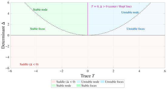
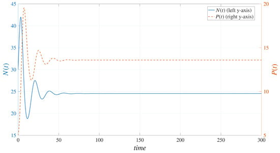
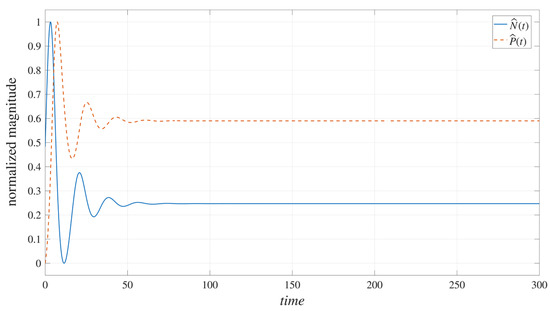
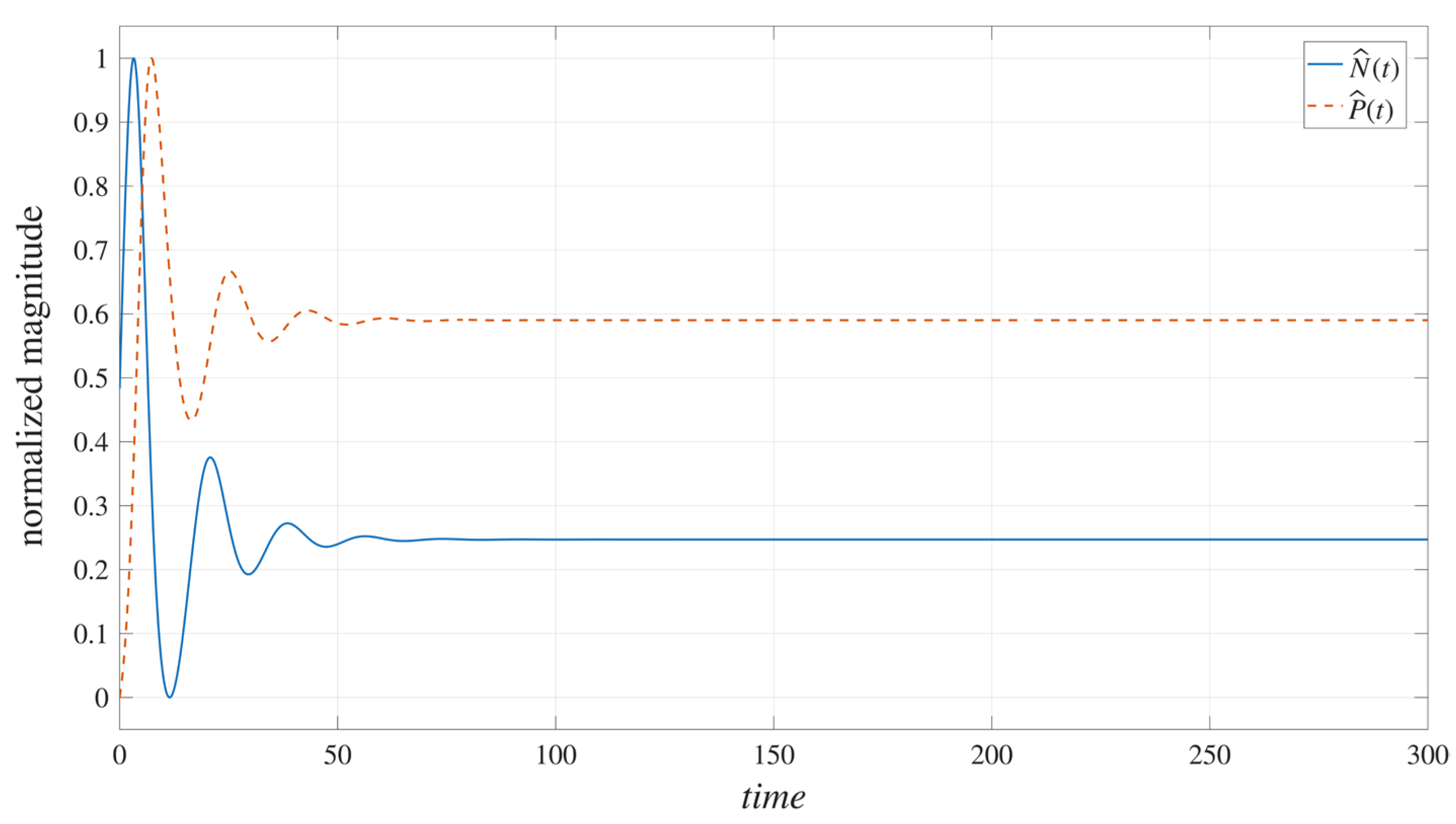
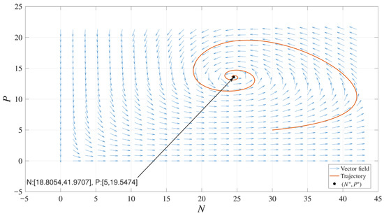
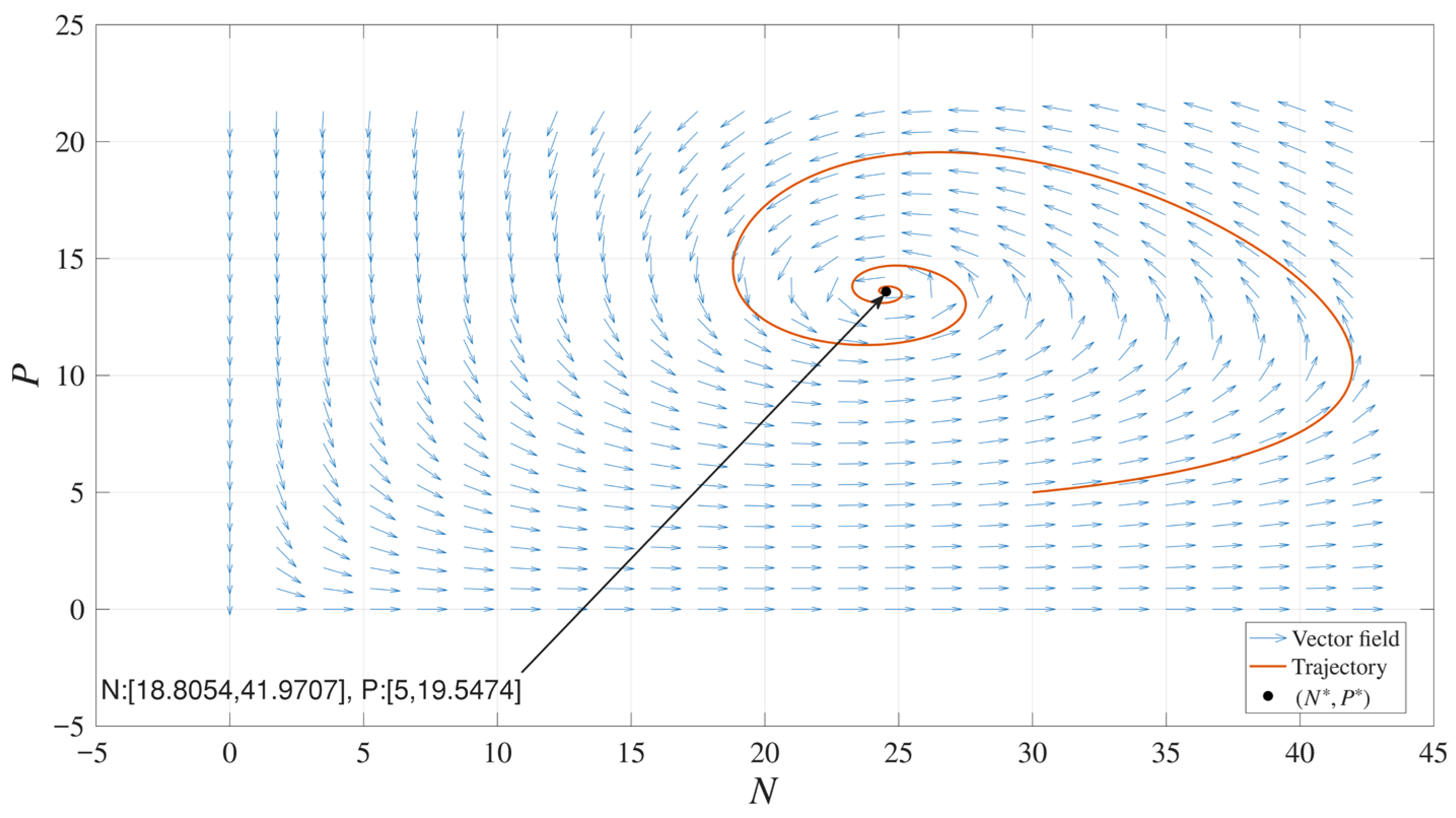
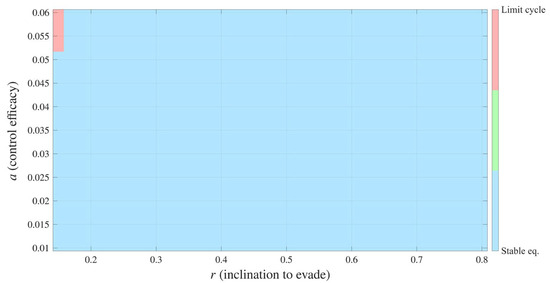
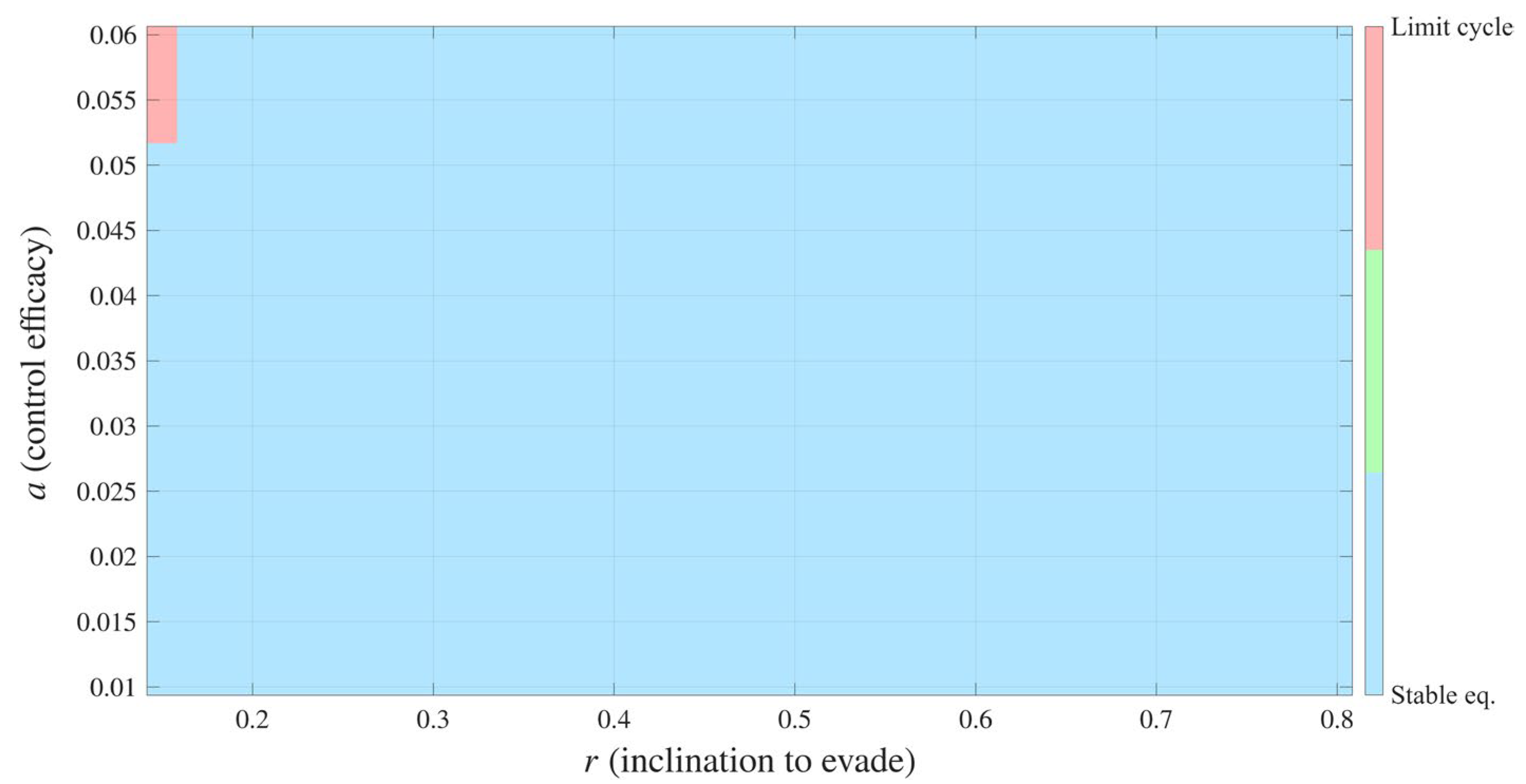
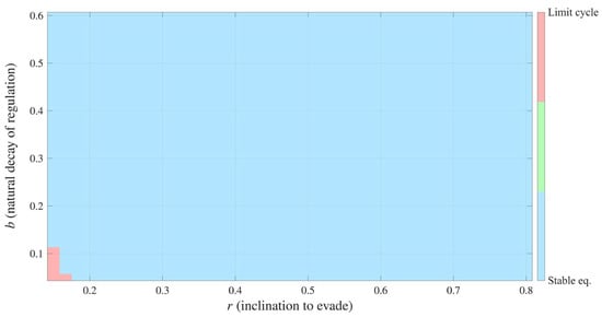
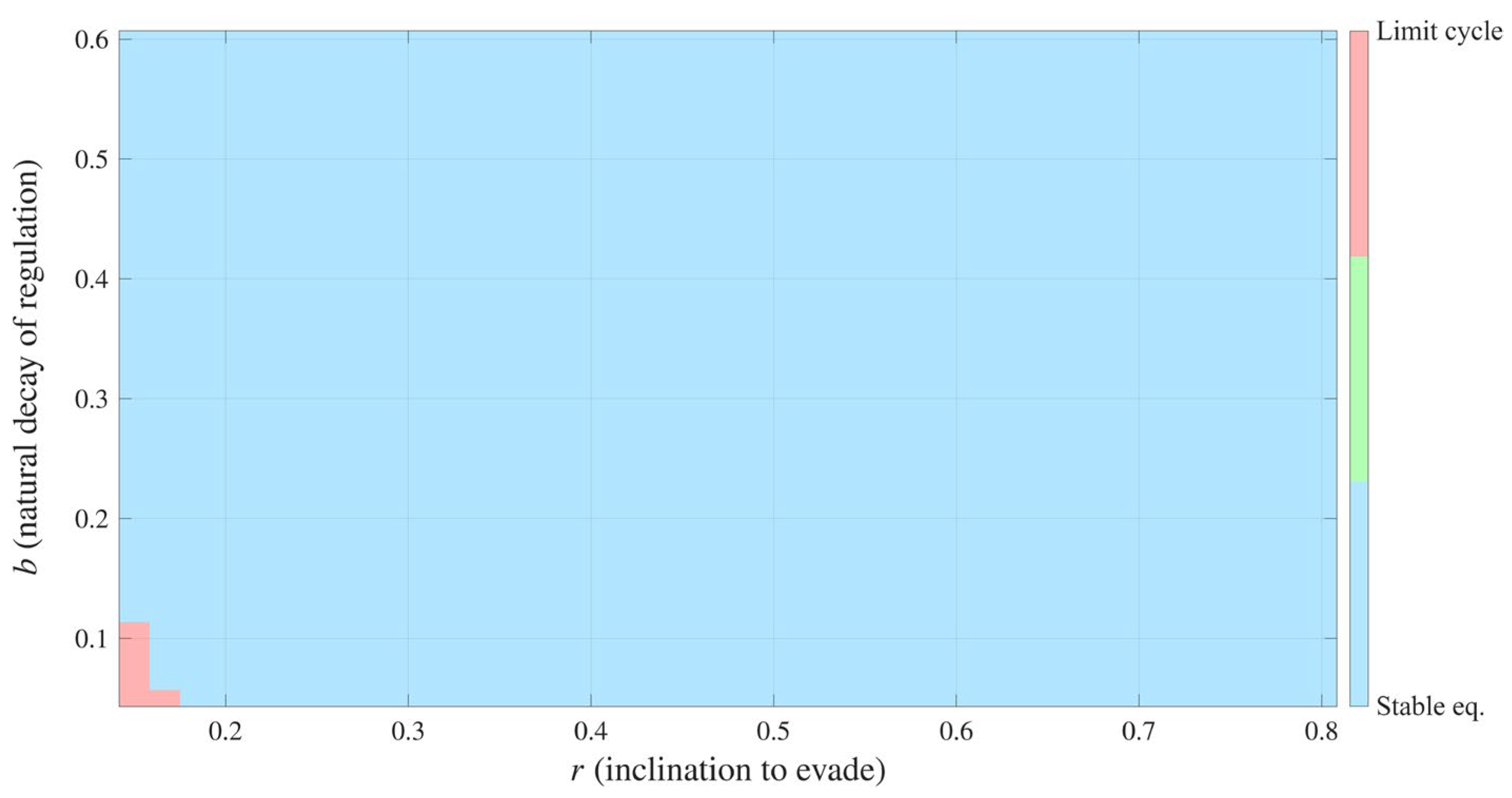
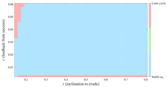
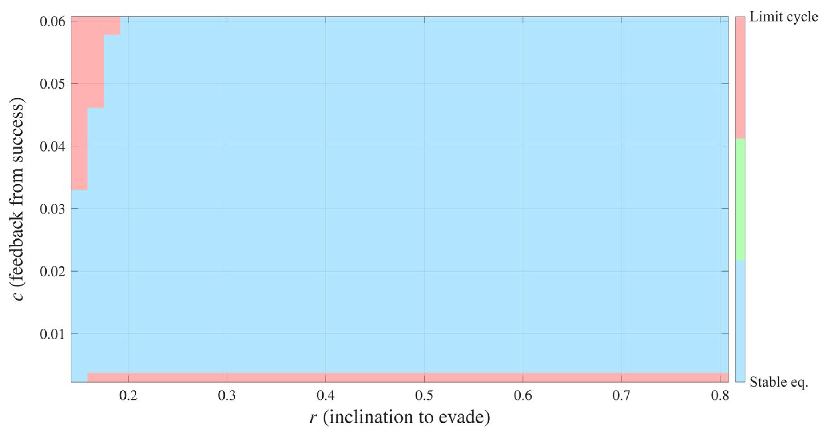
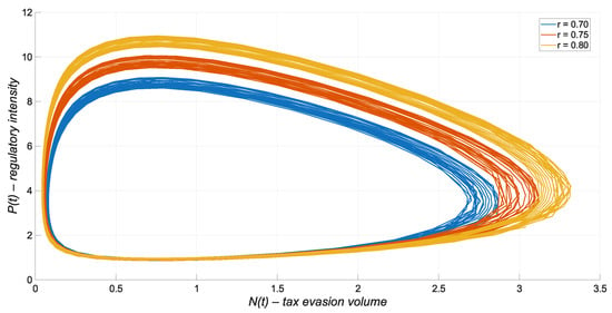
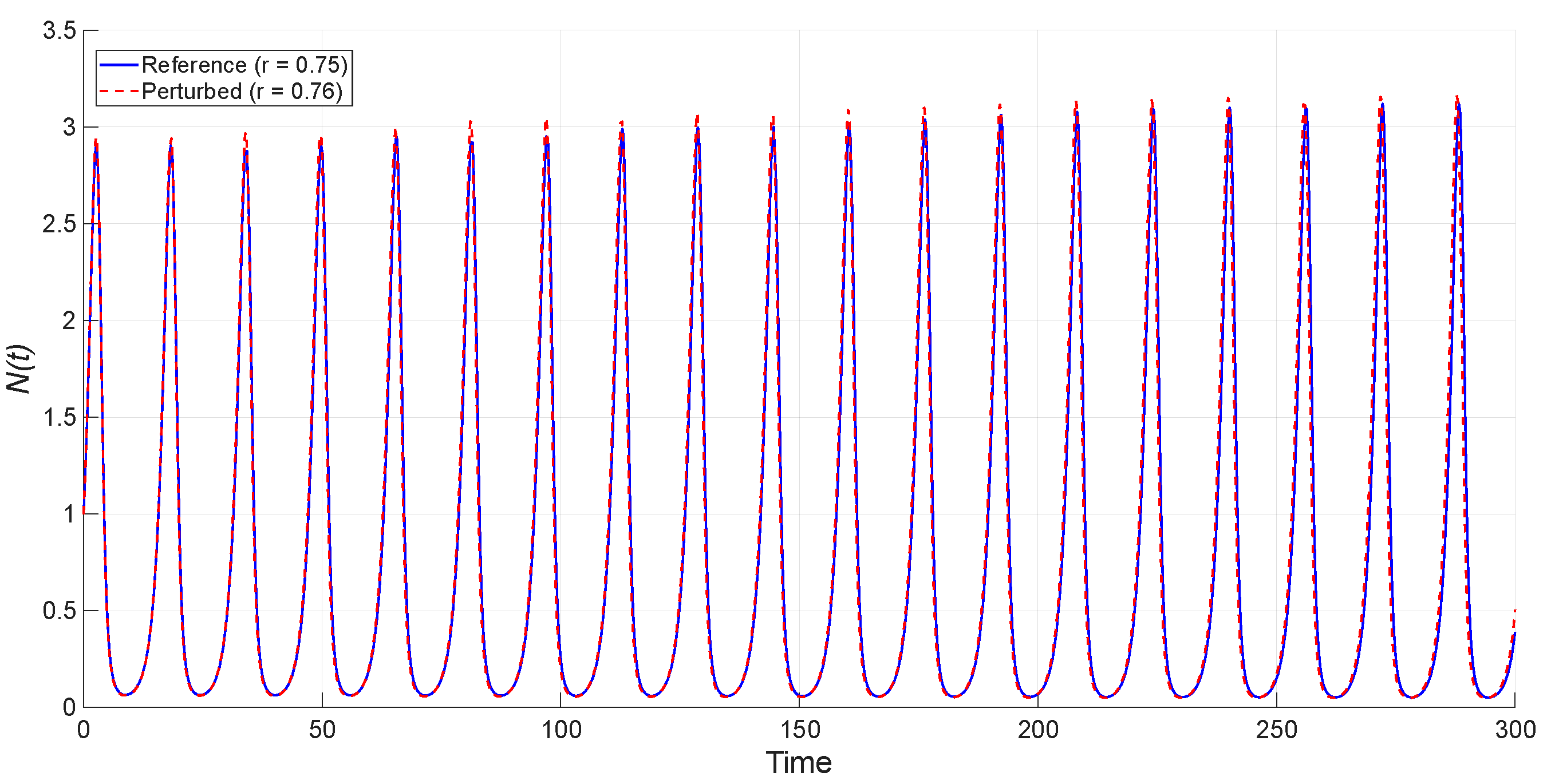
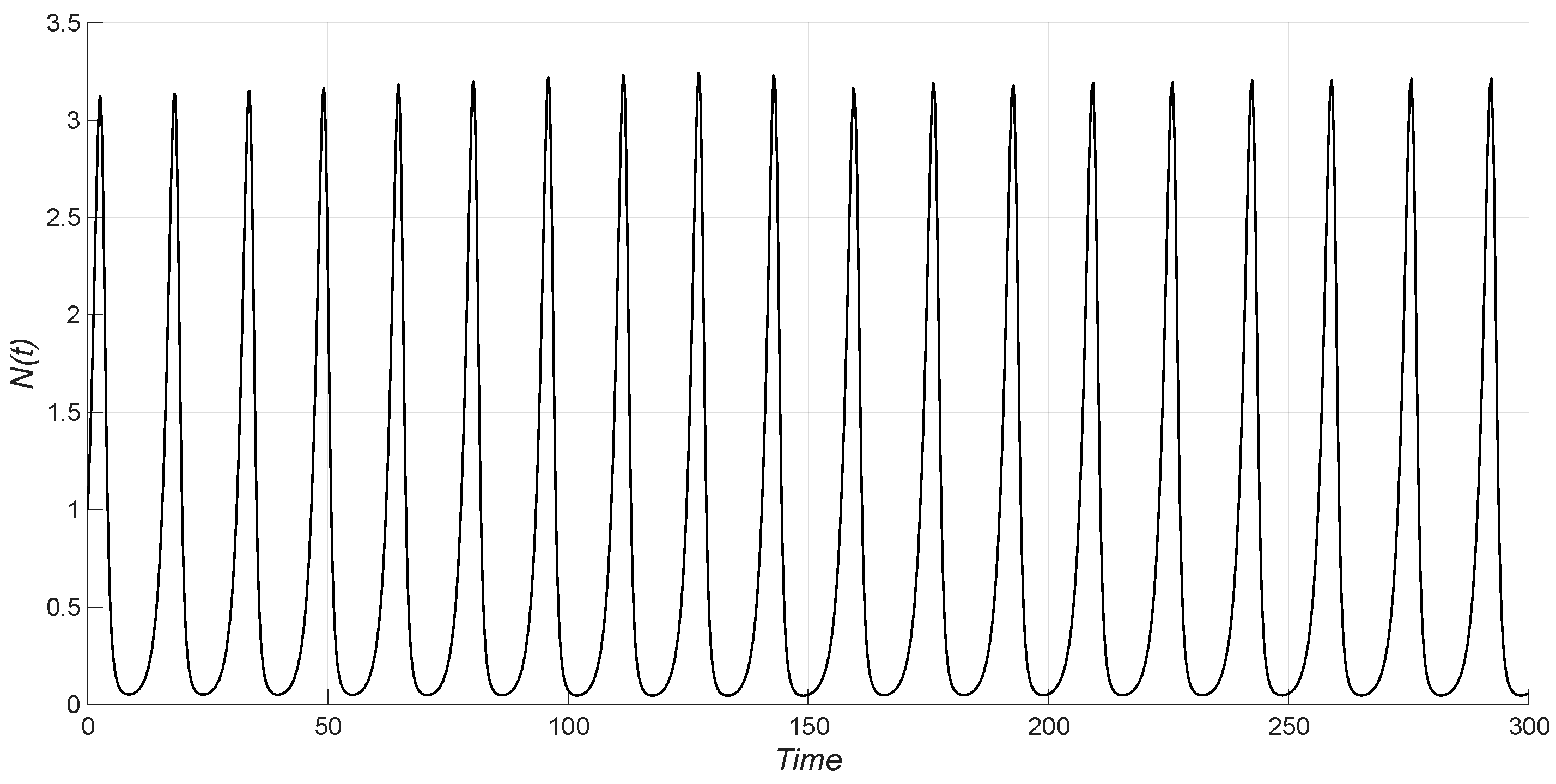

Disclaimer/Publisher’s Note: The statements, opinions and data contained in all publications are solely those of the individual author(s) and contributor(s) and not of MDPI and/or the editor(s). MDPI and/or the editor(s) disclaim responsibility for any injury to people or property resulting from any ideas, methods, instructions or products referred to in the content. |
© 2026 by the authors. Licensee MDPI, Basel, Switzerland. This article is an open access article distributed under the terms and conditions of the Creative Commons Attribution (CC BY) license.