


Abstract
Rotation-invariant (RI) point cloud models aim to reduce sensitivity to viewpoint changes, but their performance still drops noticeably in real-world settings when local geometry is degraded by noise, occlusion, and uneven sampling. Once these disturbances propagate through deeper layers, they can lead to significant robustness degradation, especially for high-capacity RI backbones. To address this problem, we propose AGSM-CPA (Adaptive Geometric Signal Modulation with Cross-Perturbation Alignment), a lightweight and plug-and-play framework that enhances the robustness of RI models without altering their core convolutional operators. It integrates two complementary modules: the Geometric Signal-to-Noise Ratio (G-SNR) modulation mechanism, which adaptively suppresses unreliable neighborhoods based on local coordinate variance, and the Cross-Perturbation Semantic Consistency Alignment (CP-SCL) module, which enforces prediction consistency between weakly augmented inputs and strongly corrupted ones. We evaluate AGSM-CPA on ModelNet40, ScanObjectNN, and ShapeNetPart. Across standard corruption protocols, AGSM-CPA consistently improves robustness while maintaining competitive clean accuracy with negligible computational overhead. These results indicate that AGSM-CPA offers a practical, reliability-aware adapter for robust rotation-invariant point cloud learning.
Keywords:
rotation-invariant point cloud learning; robust feature extraction; geometric reliability modeling; consistency learning; noise perturbation; 3D classification MSC:
93D20
1. Introduction
Three-dimensional point clouds are now a standard data format in many applications, including autonomous driving, robotics. and remote sensing [1,2]. Unlike volumetric grids or multi-view images, point clouds store spatial distributions directly. This avoids voxelization artifacts and reduces memory usage. However, this advantage comes with a cost. Point clouds are unordered, sparse, and irregular. Deep learning models therefore find it hard to learn stable features, especially when the data contains sensor noise, occlusion, or uneven sampling [3].
Point cloud learning has progressed rapidly in recent years. Early architectures such as PointNet and PointNet++ [4,5] use symmetric functions and hierarchical feature extraction to process unordered points. Later, models like DGCNN [6] and KPConv [7] introduce local graph connectivity and flexible convolution kernels to better capture neighborhood geometry. More recently, transformer-based models and large-scale pre-training have further pushed performance. Representative works include PCT [8], Point Transformer V3 [9], and Point-Mamba [10]. These models achieve strong results on benchmarks such as ModelNet40 [11]. However, these benchmarks typically use well-aligned shapes with relatively clean geometry. In practice, this ideal setting is rarely satisfied.
In real-world scenarios, data acquisition is often uncontrolled. LiDAR scans, in-the-wild 3D scans, and robotic sensing generate point clouds with two coupled challenges. First, objects can appear under arbitrary 3D rotations, and their poses are often unknown at test time. Second, the geometry itself is frequently degraded by measurement noise, background clutter, missing regions due to occlusion, non-uniform density, and quantization effects. The former calls for rotation-invariant representations; the latter requires robustness to geometric distortions. Both aspects need to be considered together in realistic systems.
In this paper, we adopt the standard definition of rotation invariance: a network’s prediction, such as a classification label or segmentation mask, should remain unchanged when the input point cloud is rotated rigidly in 3D space. This property reduces the need for heavy rotation augmentation during training and makes models more reliable when object poses are unknown or difficult to calibrate. To achieve rotation invariance, many specialized backbones have been proposed. Some methods use spherical projections or kernels [12,13]. Others build local reference frames, such as RIConv and RIConv++ [14,15] and CRIN [16]. RISurConv [17] further introduces surface-aware attention on top of rotation-invariant convolutions, and RI-MAE [18] studies self-supervised rotation-invariant pre-training.
These methods are effective in handling global pose changes on clean datasets. However, they still rely on a strong implicit assumption: the local neighborhoods used to build invariant descriptors or local reference frames are geometrically stable. When this assumption is violated, the “invariant” features can become numerically unstable. For example, PCA-based local frames may flip direction when the covariance matrix is nearly degenerate, and distance- or angle-based descriptors can vary strongly when points are missing or heavily clustered. In other words, mathematical rotation invariance does not automatically guarantee numerical stability under geometric degradation. On corrupted benchmarks such as ScanObjectNN [19], this mismatch between theory and practice often leads to significant accuracy drops for RI backbones.
In parallel, there is a growing body of work that focuses directly on robustness. PNAL [20] and DcTr [21] aim to handle noisy labels and incomplete shapes. PointDifformer [22] and SphereNet [23] learn descriptors and registration models that remain reliable under strong noise and outliers. More recent methods such as PointCVaR [24] and CausalPC [25] use risk-aware objectives and causal analysis to reweight hard or corrupted samples and improve classification robustness. However, these approaches are generally developed on top of rotation-sensitive backbones. When applied to rotation-invariant architectures, their coordinate-dependent operations may reintroduce orientation bias, thus undermining the strict invariance that such backbones aim to preserve.
This exposes a critical gap: existing rotation-invariant networks focus on handling pose variations, while robustness-oriented methods focus on mitigating noise and outliers, yet few approaches explicitly address geometric reliability under the constraint of strict rotation invariance.
To address this gap, we propose AGSM-CPA (Adaptive Geometric Signal Modulation with Cross-Perturbation Alignment), a lightweight adapter that improves the robustness of rotation-invariant backbones. Instead of redesigning the core invariant operators, which is often complex and computationally expensive, we attach two small components to existing RI networks. Our framework treats real-world distortions as a family of geometric perturbations, including Gaussian noise, background clutter, point dropout, and spatial block erasing, and explicitly trains the model to remain stable under these conditions.
The key idea is to decouple robustness into two complementary and RI-safe components: (1) local geometric reliability modeling at the feature level, and (2) cross-perturbation consistency at the prediction level.
The first component is the Geometric Signal-to-Noise Ratio (G-SNR) module. It acts as a feature-level reliability filter. For each local neighborhood, it measures the variance of relative coordinates to estimate how stable that region is. Based on this measure, it produces gating weights that down-weight unstable or noisy neighborhoods. This design is inspired by classical local geometric analysis, where PCA/covariance statistics are used to estimate surface properties and characterize stability under noise [26,27]. It is also consistent with point cloud denoising and local smoothing paradigms that rely on neighborhood statistics to suppress unreliable samples [28], as well as learning-based local geometry estimation that still implicitly depends on stable neighborhoods [29]. G-SNR is computed only from Euclidean distances, so it preserves the rotation invariance of the backbone while providing a learned, per-neighborhood confidence score. Conceptually, it plays a similar role to risk-aware reweighting in methods like PointCVaR and CausalPC, but it operates at the level of RI neighborhoods rather than whole samples.
The second component is the Cross-Perturbation Self-Consistency Alignment (CP-SCL) mechanism. It works as a prediction-level regularizer during training. The network receives two views of the same point cloud: a weakly perturbed view and a strongly perturbed view, both without extra global rotations. CP-SCL encourages the predictions for these two views to be consistent by aligning the strong-view prediction to a stop-gradient copy of the weak-view prediction. This formulation follows the established consistency learning paradigm, including teacher-student style consistency targets [30] and consistency under strong data augmentation [31]. It is also related to modern semi-supervised consistency frameworks such as MixMatch [32], but we adopt it here as a supervised robustness regularizer tailored to geometric corruptions in rotation-invariant backbones. In this way, the model learns features that remain reliable under geometric corruptions without requiring additional annotations. Unlike generic consistency pipelines designed for natural images, CP-SCL is built around a weak/strong geometric corruption gap that preserves rigid-motion assumptions while stressing local neighborhood reliability.
In summary, our contributions are as follows:
- We analyze why existing rotation-invariant networks become fragile under noise, occlusion, and uneven sampling, and identify geometric reliability as a missing factor in current RI designs.
- We propose the Geometric Signal-to-Noise Ratio (G-SNR), which estimates neighborhood stability from rotation-invariant distance statistics and modulates features accordingly, without breaking invariance.
- We integrate G-SNR with a cross-perturbation self-consistency objective (CP-SCL), forming a plug-and-play adapter for rotation-invariant backbones (e.g., RISurConv [17]). Extensive experiments validate the effectiveness of our method: on ModelNet40, it improves robustness by +2.72% under Gaussian noise () and +7.66% under 10% point dropout; on the real-scanned ScanObjectNN (PB_T50_RS), it boosts test accuracy from 93.0% to 94.65%, while adding almost no inference-time latency.
2. Related Work
Our work is related to three main research lines: deep learning on 3D point clouds, rotation-invariant representation learning, and robustness under geometric distortions. We also highlight applications in remote sensing and control, where both rotation invariance and robustness are practically required.
2.1. Deep Learning on 3D Point Clouds
Early deep models for point clouds focused on handling the unordered nature of point sets. PointNet and PointNet++ [4,5] process points independently and then aggregate them with symmetric functions, optionally in a hierarchical way. Later, graph-based and kernel-based methods such as DGCNN [6] and KPConv [7] improved local geometric modeling by building explicit neighborhoods and learning continuous filters over them.
More recent architectures adopt attention and transformer-style designs. Works like PCT [8], Point Transformer [33], and Point-BERT [34] show that self-attention can capture long-range interactions and benefit from large-scale pretraining. Very recent models such as Point Transformer V3 [9] and Point-Mamba [10] further push performance on standard benchmarks like ModelNet40 [11].
However, most of these architectures treat coordinates directly and are therefore rotation-sensitive by design. They typically rely on data augmentation to cover different poses. In addition, they often assume that local geometry is reasonably clean. When the input is heavily rotated, noisy, or sparsely sampled, early features can become unstable and difficult to interpret.
2.2. Rotation-Invariant Point Cloud Learning
Rotation-invariant (RI) methods aim to remove the dependence on global orientation. One family of approaches maps local neighborhoods onto the sphere or uses spherical harmonics, as in spherical convolutions [12,13]. Another family works directly in Euclidean space but builds features from rotation-invariant quantities such as distances and angles. RIConv and RIConv++ [14,15] are representative examples that design convolutional kernels using such invariants. CRIN [16] introduces a centrifugal reference frame to stabilize local coordinate systems, and RITR [35] extends rotation invariance to transformer-based matching. RISurConv [17] further combines RI convolutions with surface-aware attention, and RI-MAE [18] explores self-supervised rotation-invariant pretraining.
These methods focus on the pose dimension: when an object is rotated rigidly, the feature representation and prediction should not change. In theory, this is achieved by designing descriptors that depend only on rotation-invariant quantities or on local reference frames that transform consistently with the input.
In practice, however, these designs still assume that local neighborhoods are geometrically stable. When point clouds are affected by sensor noise, occlusion, or non-uniform sampling, the neighborhoods used to build local reference frames or invariant descriptors can become ill-conditioned. For example, PCA-based frames may flip direction when the local covariance matrix is close to degenerate, and distance- or angle-based descriptors can vary strongly when points are missing or clustered. As a result, even though the descriptors are formally rotation-invariant, their numerical values can become unstable under geometric degradation. This tension motivates the need to explicitly model the reliability of local neighborhoods when using RI backbones.
2.3. Robust and Reliability-Aware Point Cloud Learning
Robustness in point cloud learning has been studied from multiple, often orthogonal, perspectives, depending on the source of uncertainty. A first line of work focuses on noisy supervision, where the input geometry is assumed to be reliable but the labels are corrupted. PNAL [20] is a representative example in this category. It studies learning with noisy labels (LNL) for point cloud segmentation and proposes a two-stage framework that identifies reliable point-label pairs based on prediction consistency, followed by cluster-level label correction. In this setting, consistency is used to estimate the trustworthiness of labels, rather than the stability of geometric features. This supervision-level robustness is complementary to our work, which assumes reliable labels and instead addresses unreliability in geometric evidence.
A second line of work targets robustness to corrupted or biased inputs. Some methods focus on specific corruption types or tasks. For instance, DcTr [21] improves completion under severe corruption via a dual-channel transformer, while PointDifformer [22] and SphereNet [23] enhance robustness in registration and matching by learning noise-tolerant descriptors. These approaches typically operate on standard, rotation-sensitive backbones and do not aim to preserve strict invariance.
More recently, reliability-aware training strategies have been proposed for point cloud classification. PointCVaR [24] formulates robustness as a risk-sensitive optimization problem, emphasizing samples that dominate the tail of the loss distribution. CausalPC [25] models causal relationships between geometric features and labels to suppress spurious correlations. Both methods improve robustness by adaptive sample reweighting or causal intervention, and demonstrate strong performance under their respective evaluation settings. However, these mechanisms are defined at the sample or feature-importance level and typically rely on global statistics or absolute-coordinate attention, which makes them difficult to integrate into strictly rotation-invariant pipelines without breaking invariance.
In contrast to the above approaches, our work focuses on geometric reliability under real-world degradation. We assume that labels are reliable and that objects may undergo rotation, occlusion, and non-uniform sampling. We preserve the rotation-invariant structure of the backbone and derive reliability signals (G-SNR) exclusively from rotation-invariant statistics, such as the variance of relative distances. Furthermore, while inspired by consistency-based learning, our CP-SCL objective enforces prediction consistency under geometric perturbations to stabilize representations, rather than to filter noisy labels. As such, AGSM-CPA addresses a distinct robustness dimension that complements existing methods rather than overlapping with them.
2.4. Point Clouds in Remote Sensing and Control
The need to combine rotation invariance with robustness is especially clear in remote sensing and robotics. Road-scene LiDAR segmentation networks such as RWAFormer [1] and power line inspection methods based on UAV-mounted laser scanning [2] must handle large viewpoint changes, sensor noise, and irregular sampling all at once. Similarly, secure tracking and control systems [36,37,38] also demand robustness under dynamic disturbances and partial observability. In particular, ref. [37] investigates observer-based fault-tolerant control for nonlinear systems with actuator saturation and state constraints, highlighting the importance of stable state estimation under uncertainty, while ref. [38] surveys reinforcement learning frameworks from single-agent to multi-agent settings, emphasizing scalability and robustness in complex, real-world control environments.
Existing solutions in these domains often rely on heavy data augmentation, careful preprocessing, or task-specific heuristics to cope with both pose variation and noise. In contrast, our AGSM-CPA framework provides a generic, learning-based adapter for RI backbones: it modulates features according to local geometric stability and enforces cross-perturbation consistency during training. This makes it a promising building block for applications where both rotation invariance and robustness to real-world geometric imperfections are required.
2.5. Geometric Reliability and Consistency Regularization
Geometric reliability from local statistics. Local neighborhood statistics have long been used to estimate surface properties and assess stability under noise. Classic surface reconstruction and normal estimation methods rely on PCA/covariance analysis to derive reliable local geometry from unorganized or noisy samples [26,27]. This idea also underpins point cloud denoising and filtering methods that suppress unreliable samples using neighborhood-aware weighting [28]. Even in learning-based pipelines, robust estimation of local shape properties often assumes that neighborhoods remain sufficiently stable for meaningful aggregation [29]. Different from these works, our G-SNR is not a standalone geometry processing operator; it is a lightweight reliability gate inserted into rotation-invariant backbones, computed purely from rotation-invariant distances to avoid breaking symmetry.
Consistency learning under weak/strong perturbations. Consistency regularization has become a standard tool to improve robustness and generalization, originally popularized in semi-supervised learning. Mean Teacher [30] introduces a teacher-student consistency target (often implemented via stop-gradient or EMA teachers), while UDA [31] emphasizes enforcing prediction consistency under strong augmentations. MixMatch [32] further unifies pseudo-labeling and consistency objectives. Our CP-SCL inherits this general principle but differs in purpose and instantiation: we use consistency as a supervised robustness regularizer tailored to geometric corruptions (jitter, dropout, block erasing) on rotation-invariant point cloud backbones, explicitly constructing a weak/strong geometric severity gap rather than generic image augmentations.
3. Method
Rotation-invariant (RI) point cloud networks typically follow a hierarchical feature extraction paradigm: local geometric neighborhoods are encoded into invariant descriptors and progressively aggregated into global semantic representations. While this formulation is robust to rigid rotations, its numerical stability still depends on the quality of local geometry. In practical scenarios (e.g., real sensor data), noise, occlusion, non-uniform sampling, and missing regions may severely degrade early neighborhoods. Such imperfections distort invariant descriptors in shallow layers and can propagate through the hierarchy.
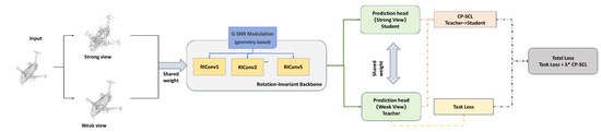
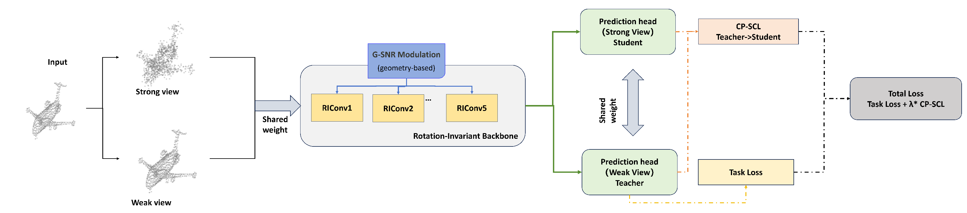
We propose AGSM-CPA, a reliability-aware enhancement framework that improves the robustness of RI backbones without modifying their rotation-invariant operators. It consists of two components: (i) Geometric Signal-to-Noise Ratio (G-SNR) feature modulation, which down-weights unreliable local neighborhoods using rotation-invariant geometric statistics; and (ii) Cross-Perturbation Semantic Consistency Alignment (CP-SCL), which enforces prediction consistency between weakly and strongly perturbed views of the same point cloud. Both components operate only on rotation-invariant quantities and introduce lightweight computation, making AGSM-CPA a plug-and-play adapter for existing RI backbones (see Figure 1).
Figure 1.
Overall pipeline of AGSM–CPA.Given an input point cloud, we construct a weakly perturbed view and a strongly perturbed view, which are processed by a shared rotation-invariant backbone augmented with G-SNR modulation. The weak view serves as a teacher branch supervised by the task loss, while the strong view acts as a student branch aligned to the teacher prediction via cross-perturbation semantic consistency learning (CP-SCL). G-SNR is applied at intermediate layers to modulate feature magnitudes based on local geometric reliability, while the backbone architecture and rotation-invariant operators remain unchanged.
3.1. Overview
Let be an input point cloud, where denotes the 3D coordinates of the i-th point (i.e., “xyz”). A rotation-invariant backbone produces per-point features , and a task head outputs class probabilities for C classes (with the probability simplex).
AGSM-CPA augments by attaching a point-wise reliability gate at intermediate layers (G-SNR) and adding a prediction-level consistency term during training (CP-SCL). Concretely, at an RI block ℓ, the backbone outputs per-point features , where is the number of points after possible downsampling. G-SNR computes a scalar reliability score from local geometric dispersion and modulates the feature magnitude. At the output level, CP-SCL constructs two perturbed views and aligns their predictions , using the weak-view prediction as a teacher signal.
3.2. Preliminaries: Rotation-Invariant Backbones
At layer ℓ, an RI backbone builds a -NN neighborhood for each point:
where typically increases with depth. Since Euclidean distances are preserved under rigid rotations, is rotation-invariant.
A generic RI block can be expressed as
where is constructed from rotation-invariant primitives (e.g., distances, angles, normalized offset norms) and is a permutation-invariant aggregator. Although (2) is formally rotation-invariant, its numerical stability depends on the quality of local neighborhoods, motivating explicit reliability modeling.
3.3. G-SNR: Feature-Level Reliability Modulation
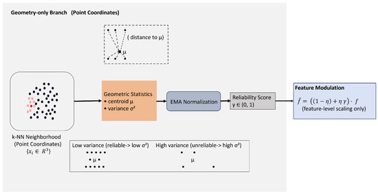
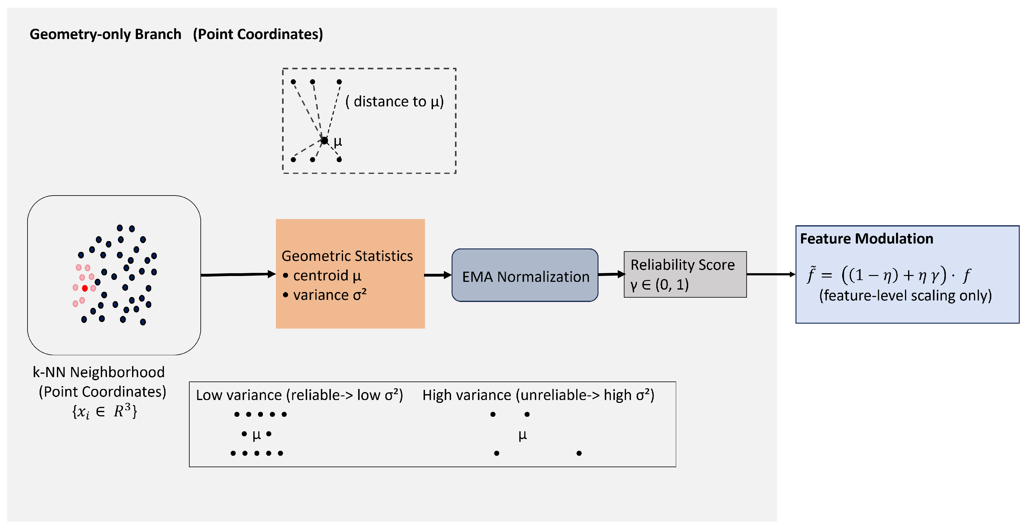
As illustrated in Figure 2, G-SNR estimates a geometry-only scalar reliability score from local neighborhood statistics and applies it as a lightweight feature-level modulation without modifying any rotation-invariant operators.
Figure 2.
Geometry-only reliability estimation in G-SNR. For each point, G-SNR computes local geometric statistics—namely the neighborhood centroid and variance —solely from point coordinates within a k-NN neighborhood. After EMA-based normalization, a scalar reliability score is obtained, reflecting the stability of local geometry. This reliability score is used only for feature-level scaling and does not alter neighborhood construction, aggregation, or any rotation-invariant operators in the backbone.
For each point , we compute the neighborhood centroid
and the neighborhood variance (dispersion)
where is the Euclidean norm.
To stabilize the scale across layers and datasets, we maintain an exponential moving average (EMA) baseline of batch-mean variance:
where is the EMA decay and is the mean of over the current mini-batch (and points at layer ℓ).
- EMA stability and the role of .
Equation (5) maintains an exponential moving average (EMA) baseline of the batch-mean variance. For a fixed layer ℓ, denote the observed batch statistic at step t as and the EMA baseline as . Unrolling the recurrence yields
showing that older batch statistics are exponentially down-weighted by . Under the standard assumption that has bounded variance and weak cross-batch correlation, the variance of the EMA estimator admits the asymptotic bound
which indicates that larger yields a smoother and more stable normalization baseline. We empirically validate the batch-wise stability and layer-wise consistency under different in Section 4.5.3, and provide a theoretical convergence analysis in Appendix A.
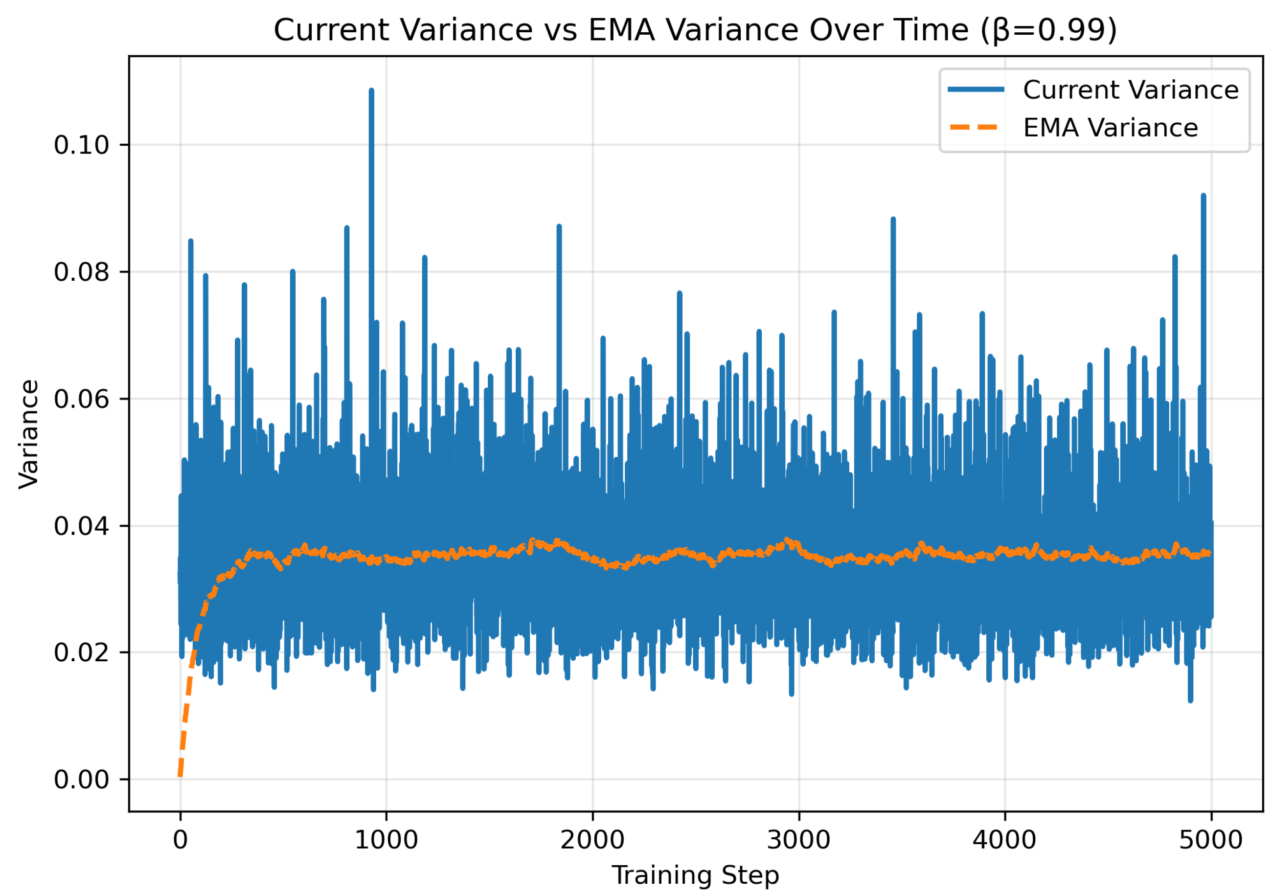
For clarity, in our implementation we log the instantaneous batch statistic as cur_var, the EMA baseline as ema_var, and the resulting residual gate values in Equation (10) as gate. These logs enable a direct empirical verification of the smoothing behavior implied by Equation (6) and the stability trend predicted by Equation (7).
We then define the normalized variance
and the geometric signal-to-noise ratio (G-SNR) reliability score
- Residual reliability gate.
Given the backbone feature , G-SNR applies a lightweight residual modulation:
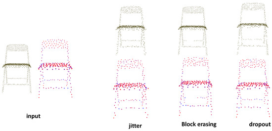
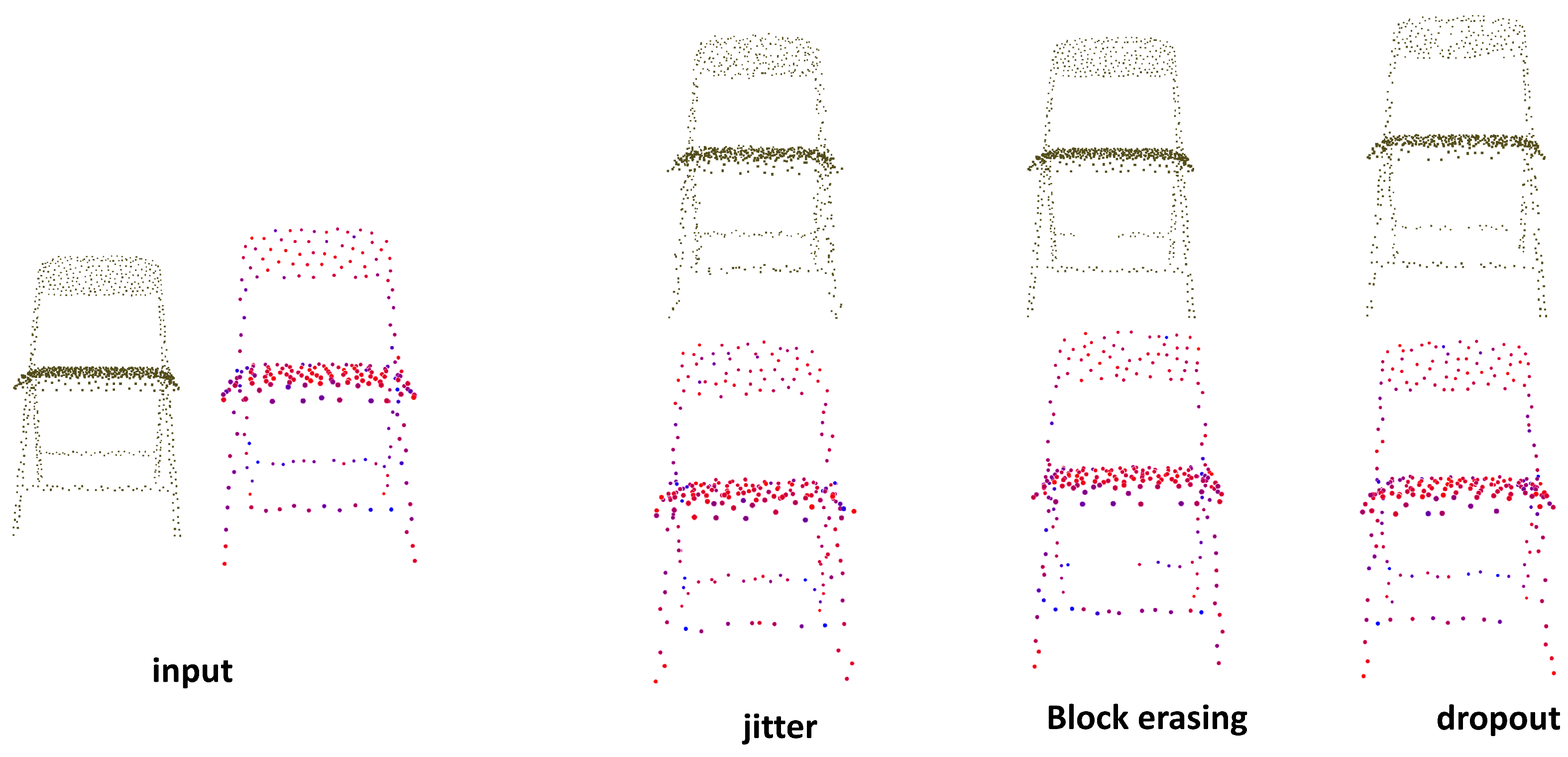
where controls the gate strength (default ). Figure 3 visualizes the behavior of G-SNR under increasing geometric degradation, showing that unreliable regions are consistently down-weighted while stable structures preserve higher reliability scores.
Figure 3.
Response of G-SNR gate under different geometric perturbations. Points are colored by the G-SNR gate scalar at a shallow layer (warmer colors indicate higher reliability weights). Under mild perturbations (jitter), most surface regions retain high confidence. As geometric degradation increases (random dropout and block erasing), G-SNR consistently assigns lower weights to sparse, irregular, or missing regions, while preserving stable structural parts. This behavior confirms that G-SNR acts as a geometry-only reliability estimator rather than a semantic or coordinate-dependent attention mechanism.
- Rotation invariance preservation.
Let be any rigid rotation. Under , Euclidean distances and hence k-NN sets (1) are unchanged; moreover, the centroid (3) rotates as , and implies the variance (4) is invariant. Therefore in (8) and in (9) are rotation-invariant scalars. Finally, (10) rescales by a scalar that does not depend on orientation, so G-SNR does not alter the backbone’s rotation-invariant mapping.
3.4. CP-SCL: Cross-Perturbation Semantic Consistency Alignment
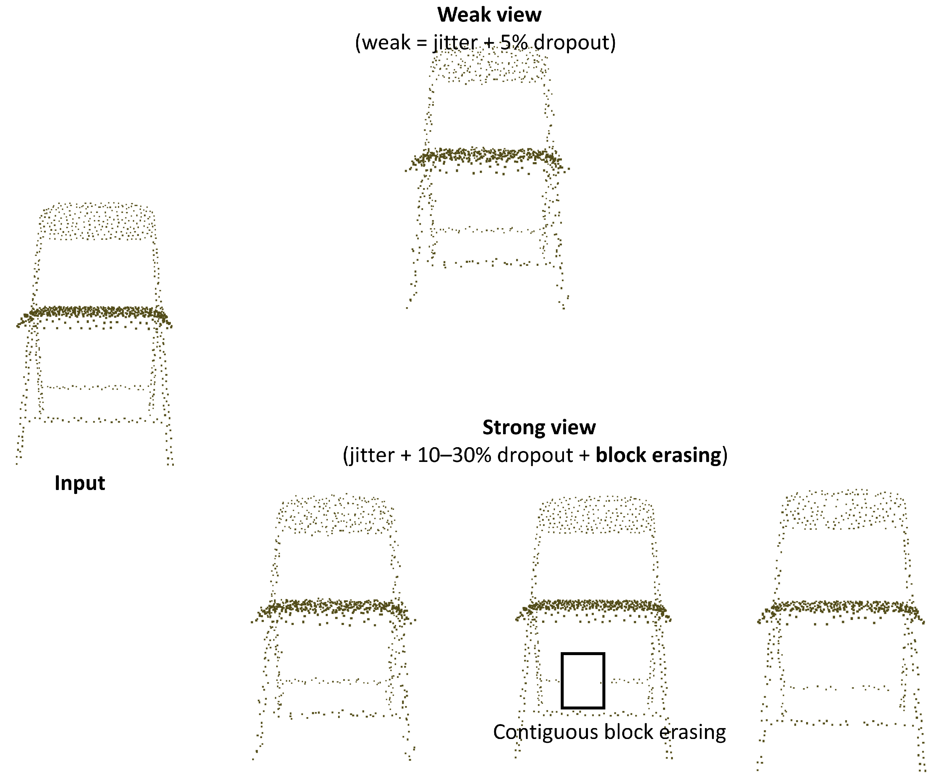
For each input P, we construct two perturbed views: a weak view (mild jitter and light dropout) and a strong view (heavier corruption, e.g., random point dropout, contiguous block erasing, and stronger jitter). Importantly, and are orientation-agnostic perturbations: they do not rely on any canonical alignment, nor do they inject extra user-defined rotation augmentation. Therefore, they do not introduce an orientation bias beyond the benchmark protocol, and the consistency term is evaluated on top of the rotation-invariant backbone.
Feeding both views into the same backbone and head yields probability vectors and . We treat the weak-view prediction as a teacher and align the strong-view prediction as a student by a KL divergence:
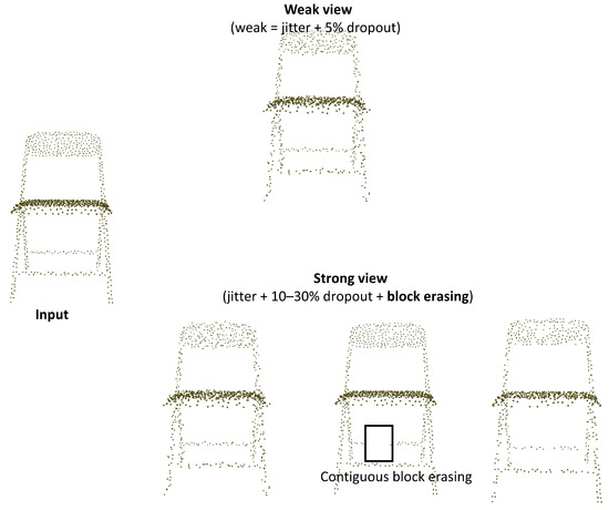
where stops gradients for the teacher branch in the consistency term. The weak branch still receives gradients from the supervised task loss. As illustrated in Figure 4, the weak and strong views differ mainly in the severity of geometric perturbations, with the strong view introducing spatially coherent block erasing in addition to random dropout and jitter.
Figure 4.
Illustration of weak and strong perturbations (). Starting from the same input point cloud (left), the weak view applies mild geometric noise (light jitter and low-rate random dropout), preserving most local structures. The strong view introduces heavier corruptions, including higher dropout rates and contiguous block erasing, which removes spatially coherent regions of points. These perturbations are orientation-agnostic and do not rely on any canonical alignment, making them compatible with rotation-invariant backbones.
- Rotation invariance of the objective.
Since the backbone is rotation-invariant and our perturbations are orientation-agnostic (i.e., not tied to a canonical frame), the consistency objective in (11) does not encourage any particular orientation and remains compatible with symmetry.
3.5. Training Objective and Procedure
We train with the standard supervised task loss on the weak view and add CP-SCL as a regularizer:
where is cross-entropy, y is the ground-truth label, and controls the consistency weight (default ). To avoid contaminating the variance baseline with heavy corruptions, we update the EMA statistic using the weak branch only (see Algorithm 1).
| Algorithm 1: Training procedure of AGSM-CPA (G-SNR enabled layers ) |
|
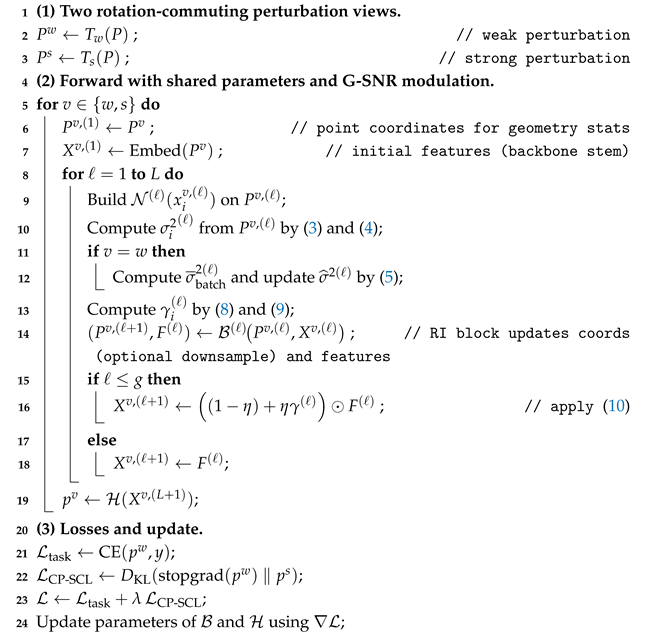 |
3.6. Complexity Discussion
G-SNR introduces only neighborhood statistics and a scalar gate. Since RI backbones already construct -NN neighborhoods, the additional cost is the computation of (3) and (4),which is per layer ℓ and negligible compared with typical feature MLP/attention operations. The gate (10) is an elementwise scaling. CP-SCL doubles the forward pass during training (two views) but does not change inference-time complexity.
- Parameter sensitivity.
Key hyperparameters include (EMA decay), (gate strength), and (consistency weight). We provide a sensitivity analysis over these parameters in Section 4.5.
4. Experiments
This section presents a comprehensive evaluation of the proposed AGSM-CPA framework. We study its effectiveness from three perspectives: (1) standard classification performance on clean datasets, (2) robustness to noise, point dropout, and structural corruption, and (3) generalization to part segmentation. Unless otherwise stated, all experiments are conducted on RISurConv-based backbones. Across all settings, AGSM-CPA consistently improves stability and generalization with almost negligible parameter overhead.
4.1. Datasets
ModelNet40 [11] contains 12,311 clean CAD models from 40 object categories. Following the standard protocol, we use 9843 models for training and 2468 for testing. All point clouds are normalized to the unit sphere and uniformly sampled to a fixed number of points.
ScanObjectNN [19] is a real-scanned dataset designed to evaluate robustness under noisy, cluttered, and occluded indoor scenes. We follow the most challenging PB_T50_RS variant for all comparisons, which introduces background points, random translations, and rotations.
ShapeNetPart [39] contains 16 object categories and 50 part labels with point-level annotations. It is used to evaluate whether the robustness improvements brought by AGSM-CPA on classification tasks can transfer to fine-grained part segmentation. We report category-wise part mIoU.
4.2. Implementation Details
All models are implemented in PyTorch (version 2.6.0) and trained on a single NVIDIA A100 GPU. Unless otherwise stated, we adopt RISurConv as the rotation-invariant (RI) backbone and integrate AGSM-CPA by (i) inserting G-SNR gates into the first RI blocks, and (ii) optimizing with the proposed CP-SCL objective using a weak/strong view pipeline. All hyperparameters not explicitly mentioned follow the default settings of the RISurConv codebase.
- Optimization.
We use a total batch size of 32 and the Adam optimizer with an initial learning rate of . The learning rate follows cosine decay without restarts. We train for 450 epochs on ModelNet40 and ScanObjectNN. For ShapeNetPart, we follow the default RISurConv training schedule and plug in AGSM-CPA without additional tuning.
- G-SNR and CP-SCL defaults (symbol consistency with Section 3).
Unless otherwise stated, the residual gate strength is set to in Equation (10), the EMA decay is in Equation (5), and the consistency weight is in Equation (12). G-SNR is enabled in the first RI blocks (Equation (10)); deeper blocks keep the original backbone features.
- Perturbation pipeline ().
During training, each input point cloud is transformed into a weak view and a strong view for CP-SCL (Equation (11)). The weak view uses light jitter (Gaussian noise with ) and low-rate random dropout (5%). The strong view combines: (i) random point dropout (default 10%, with a maximum of 30% in the strong-view sampling range), (ii) block erasing, and (iii) Gaussian jitter ().
For block erasing, we apply it with probability per sample. A cuboid occlusion is generated by sampling each side length independently from times the corresponding bounding-box extent, and all points inside the cuboid are removed. We then resample (with replacement) from the remaining points to keep the input size fixed; if fewer than points remain after erasing, the operation is skipped. This design produces spatially coherent occlusions while preserving batch consistency and matches common missing-region patterns in real-world scans.
Rationale. We choose the weak/strong ranges to create a clear structural-severity gap while avoiding degenerate inputs: remains close to the clean geometry to provide a stable teacher signal, whereas applies substantially stronger but still shape-preserving corruptions. The minimum-remaining-point check (skip if fewer than points remain) and the fixed-size resampling ensure that strong-view perturbations do not collapse the input and keep the optimization stable and reproducible.
- Rotation augmentation and invariance.
We do not apply additional user-defined rotation augmentation during training, since RISurConv is rotation-invariant by design and we aim to isolate the contribution of AGSM-CPA from explicit symmetry augmentation. Note that ScanObjectNN (PB_T50_RS) includes random translation/rotation as part of the dataset protocol; our statement “no rotation augmentation” refers to not injecting any extra rotation beyond the benchmark definition.
All augmentations in are jitter/occlusion-type perturbations that do not rely on any canonical orientation or extra rotation augmentation; thus the evaluation isolates the contribution of AGSM-CPA on top of the RI backbone.
- Efficiency and overhead.
To quantify overhead, we report parameter count, GFLOPs, relative training time per epoch, and single-sample inference latency (ms) measured on an NVIDIA A100 under the same batch size and input resolution. “Train time/epoch” includes the two-view forward pass required by CP-SCL during training, while “Inference” is measured with a single view and thus reflects deployment-time cost. “+G-SNR only” disables CP-SCL (), and“+CP-SCL only” removes G-SNR gating (i.e., the gate is an identity mapping with , and no reliability modulation is applied), “Full AGSM-CPA” enables both modules with the default settings above.
Table 1 shows that AGSM-CPA is lightweight in both parameters and computation. All variants have essentially identical parameter counts and GFLOPs because G-SNR introduces only scalar gating and neighborhood statistics (computed on top of existing k-NN neighborhoods), while CP-SCL does not change the backbone architecture. The main training-time overhead comes from the two-view pipeline required by CP-SCL, leading to ∼1.2–1.25× relative time per epoch. Importantly, inference latency remains almost unchanged (within ∼1 ms), since CP-SCL is applied only during training and G-SNR adds only a negligible per-point scaling at inference.
Table 1.
Efficiency and overhead of AGSM-CPA variants. All variants share the same RISurConv backbone and differ only in the attached modules. Training time is reported as relative time per epoch (Baseline = 1.0×).
4.3. ModelNet40 Evaluation
4.3.1. Clean Classification Performance
We first evaluate AGSM-CPA on clean ModelNet40 classification to verify that a robustness-oriented design does not compromise standard recognition accuracy. This experiment serves as a steady-state capability check rather than a state-of-the-art comparison.
Table 2 evaluates whether robustness-oriented design harms standard recognition. We compare RISurConv with and without AGSM-CPA under the same RI backbone and training schedule. AGSM-CPA slightly improves clean accuracy (+0.4%), suggesting that suppressing unreliable local geometry can benefit representation quality even under nominally clean conditions, without introducing a clean vs. robust trade-off.
Table 2.
Clean classification accuracy on ModelNet40. “xyz” denotes raw 3D coordinates and “nor” denotes per-point surface normals.
4.3.2. Robustness Under Controlled Corruptions
We next evaluate robustness on ModelNet40 under controlled synthetic corruptions, including Gaussian noise, random point dropout, and structured block dropout. These perturbations are applied only at test time. This setting isolates the model’s response to increasing geometric uncertainty and provides a controlled bridge from clean benchmark evaluation to real-world robustness.
As shown in Table 3, AGSM-CPA consistently outperforms the RISurConv baseline across all corruption types. Notably, the performance gap grows as the corruption becomes more severe, particularly under point dropout and block dropout, which simulate partial observations and occlusions. Rather than claiming that synthetic corruptions fully capture real-world scanning artifacts, this experiment establishes a clear trend: as geometric uncertainty increases, reliability-aware learning yields increasingly stable predictions. We next validate this effect on real-scanned point clouds.
Table 3.
Robustness evaluation on ModelNet40 under controlled test-time corruptions.
4.3.3. Complementary Robustness: A Scenario-Wise Analysis
Protocol for scenario-wise evaluation. For Scene A (tail risk), we report mean accuracy, worst-class accuracy, and CVaR@10% computed over per-sample classification losses on the test set. For Scene B (bias shift), we introduce a label-correlated geometric artifact during training and remove it at test time; the ID/OOD split follows the same classes with and without the artifact. For Scene C (geometric reliability degradation), we evaluate quantization (coordinate rounding to 10-bit resolution), mixed corruption (randomly sampling one corruption type per sample from a predefined set), and local dropout (structured removal within local neighborhoods). Full details are provided in Appendix A.
Robustness in point cloud learning is a multi-faceted challenge, where different failure modes demand specialized solutions. To precisely delineate the contribution of AGSM-CPA and address the question of novelty, we conduct a scenario-wise analysis that distinguishes three primary sources of uncertainty: (A) sample-level tail risk, (B) spurious causal bias, and (C) geometric reliability degradation. The key insight is that state-of-the-art methods excel in their designed scenarios but do not generalize across all. This analysis moves beyond claiming universal superiority and instead clarifies the complementary roles of different robustness paradigms. For fair comparison, all robustness objectives (PointCVaR, CausalPC, and AGSM-CPA) are implemented as plug-in training strategies on the same RISurConv backbone and evaluated under identical data and optimization protocols.
- Reliability note (Scenes A–C).
To reduce run-to-run randomness, we evaluate all methods using multiple random seeds under identical training and evaluation settings. For each metric, we report mean±std across runs and assess robustness trends based on consistent performance differences. Our goal in this scenario-wise analysis is to characterize complementary robustness behaviors rather than to claim universal statistical dominance; therefore, we interpret numerical gaps conservatively and avoid over-interpreting marginal differences.
- Scene A: Sample-level Tail Risk.
PointCVaR [24] is explicitly designed to handle scenarios where errors are dominated by a small fraction of high-loss samples, such as class imbalance or adversarially selected hard instances. We evaluate robustness under tail-risk-dominated settings using worst-case and CVaR-based metrics.
In Table 4, “Mean Acc.” denotes overall classification accuracy, while “Worst-class Acc.” reflects the minimum per-class accuracy across categories. “CVaR@10%” is computed by averaging the worst per-sample losses, emphasizing tail behavior. As expected, PointCVaR achieves the strongest robustness on tail-focused metrics due to its explicit risk-sensitive objective. AGSM-CPA maintains competitive mean accuracy but does not target tail minimization, which aligns with its design intent. Across multiple runs, the relative ordering of methods remains consistent, and PointCVaR exhibits the most pronounced advantage on worst-case metrics.
Table 4.
Scene A: Tail-risk robustness on ModelNet40.
- Scene B: Spurious Correlation and Bias Shift.
CausalPC targets robustness against shortcut learning induced by spurious correlations. We simulate a bias-shift scenario by injecting label-correlated artifacts during training and removing them at test time.
CausalPC substantially reduces the ID–OOD performance gap, confirming its effectiveness in mitigating spurious correlations. AGSM-CPA improves over the baseline but does not fully close the gap, reflecting its different design objective. Across multiple runs, the ID–OOD gap for CausalPC remains consistently smaller than that of AGSM-CPA and RISurConv, indicating robust causal generalization, please refer to Table 5.
Table 5.
Scene B: Robustness under spurious causal bias on ModelNet40.
- Scene C: Geometric Reliability Degradation.
We next evaluate robustness under localized geometric perturbations, including quantization, mixed corruption, and structured point removal, see as Table 6.
Table 6.
Scene C: Robustness under geometric reliability degradation on ModelNet40.
Under all three geometric corruption settings, AGSM-CPA consistently outperforms prior methods. The performance gap widens as the corruption becomes more structurally disruptive, highlighting the benefit of explicitly modeling geometric reliability. These results suggest that AGSM-CPA targets a distinct robustness dimension that is complementary to both tail-risk mitigation and causal debiasing.
This scenario-wise evaluation reveals a complementary robustness landscape: PointCVaR is most effective for tail-risk mitigation, CausalPC excels at suppressing spurious correlations, and AGSM-CPA uniquely addresses geometric reliability degradation. Together, these results clarify that AGSM-CPA is not a variant of existing approaches but instead targets a distinct and practically important failure mode in rotation-invariant point cloud learning.
4.4. Classification on ScanObjectNN
We next evaluate AGSM-CPA on ScanObjectNN (PB_T50_RS), a challenging real-world benchmark composed of object-level point clouds with clutter, occlusion, background points, and non-uniform sampling. Compared with ModelNet40, ScanObjectNN exhibits stronger geometric degradation and distribution shift between training and testing data.
- Overall performance and generalization gap.
Table 7 reports training accuracy, test accuracy, and the generalization gap (Train–Test). AGSM-CPA consistently improves test performance over the RISurConv backbone while reducing the generalization gap from to percentage points.
Table 7.
Classification performance on ScanObjectNN (PB_T50_RS).
The reduced generalization gap indicates that AGSM-CPA mitigates overfitting to dataset-specific geometric patterns. By enforcing consistency between weakly and strongly perturbed views during training, CP-SCL acts as an implicit structural regularizer, discouraging reliance on fragile local configurations that do not generalize to unseen scans.
- Robustness under varying geometric degradation.
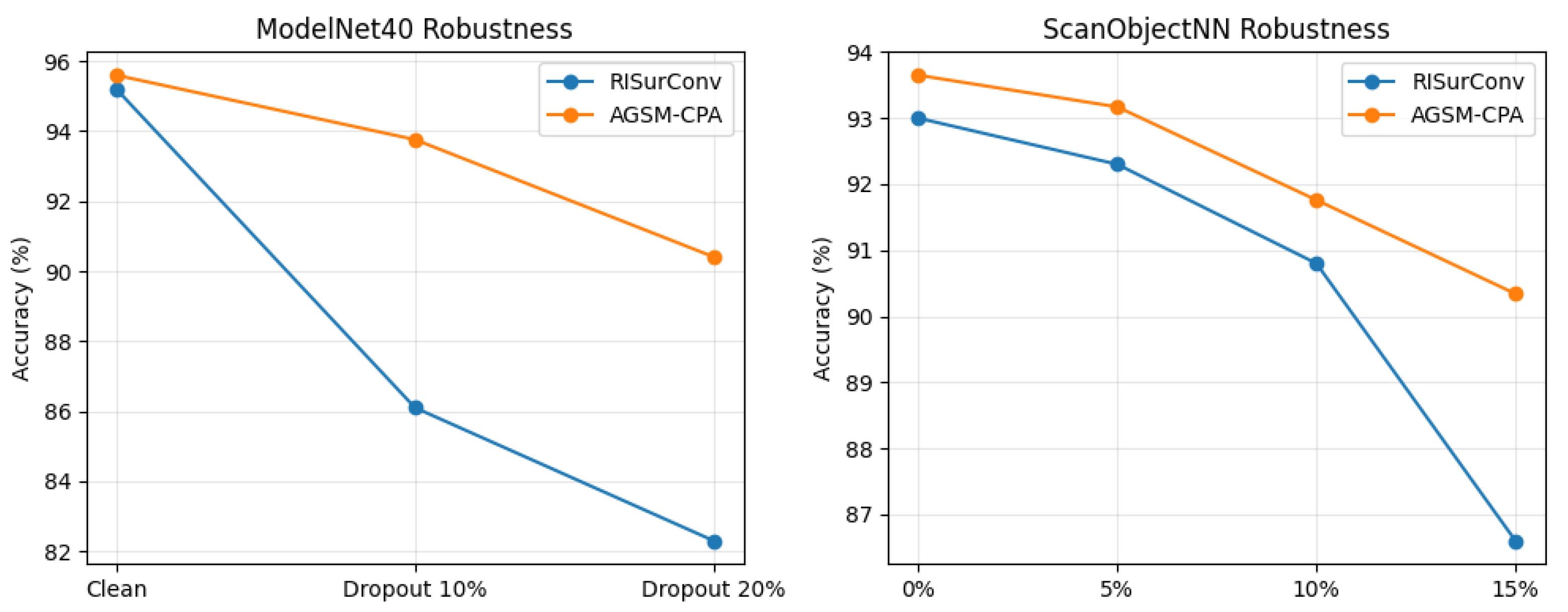
Table 8 shows that AGSM-CPA consistently outperforms the RISurConv baseline across all levels of geometric degradation. More importantly, the performance gap between the two methods widens substantially as corruption intensifies, indicating that AGSM-CPA degrades in a more controlled and progressive manner when local geometry is compromised. While the baseline model exhibits a rapid accuracy drop under increasing point removal and noise, AGSM-CPA maintains high recognition accuracy until severe structural damage occurs.
Table 8.
Robustness trends on ScanObjectNN under geometric degradation.
The robustness under mild degradation is particularly noteworthy. With only 5% random point dropout, AGSM-CPA preserves high accuracy (93.17%), showing no sign of performance collapse. We attribute this behavior not to test-time regularization, but to the training strategy of CP-SCL, which explicitly exposes the model to structurally incomplete views. As a result, the network becomes less sensitive to moderate point removal at inference time, treating such degradation as a familiar variation rather than a distribution shift. This observation supports the interpretation of CP-SCL as a form of structure-aware regularization, rather than aggressive or adversarial data augmentation.
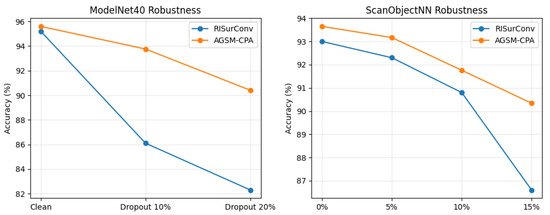
To better visualize the progressive degradation reported in Table 8, we plot the accuracy trends as corruption severity increases in Figure 5. AGSM-CPA exhibits a more gradual degradation curve than the RISurConv baseline on both ModelNet40 and ScanObjectNN, indicating improved robustness under increasing geometric perturbations.
Figure 5.
Robustness trends under increasing geometric degradation. (Left): ModelNet40 accuracy under increasing point dropout. (Right): ScanObjectNN accuracy under increasing corruption severity. AGSM-CPA degrades more gradually than the RISurConv baseline, demonstrating improved robustness under both synthetic and real-world perturbations.
- Hyperparameter settings and sensitivity.
Unless otherwise specified, AGSM-CPA follows the default RISurConv configuration. The neighborhood size is selected from the standard set across layers. For G-SNR, the EMA decay in Equation (5) is fixed to to maintain a stable variance baseline for normalization. For CP-SCL, we use the default consistency weight and the weak/strong perturbation pipeline described in Section 4.2. In the strong view, random point dropout is used as part of : we use a default dropout ratio of 10% during training (together with block erasing and jitter), and we additionally evaluate broader dropout levels at test time in Table 8.
We find that aggressively reducing k (to half of the default) destabilizes local statistics and severely hurts performance, as neighborhoods become too small to capture reliable geometric structure. Conversely, moderately increasing k (to twice the default) yields comparable accuracy on ScanObjectNN but does not provide consistent gains, indicating diminishing returns from excessively large neighborhoods that may dilute local geometric cues. Overall, AGSM-CPA exhibits stable behavior within a reasonable hyperparameter range and does not rely on careful tuning to achieve strong performance.
The ScanObjectNN benchmark primarily presents challenges of localized geometric degradation, including occlusion, background clutter, and incomplete observations, rather than global noise or systematic label bias. This setting aligns precisely with the geometric reliability scenario identified in our earlier analysis. The strong performance of AGSM-CPA on ScanObjectNN highlights the effectiveness of its two core mechanisms: local geometric reliability modeling via G-SNR and cross-perturbation consistency learning via CP-SCL.
Together, these results confirm that AGSM-CPA targets a critical and previously underexplored robustness dimension in point cloud learning. This dimension is complementary to tail-risk minimization approaches such as PointCVaR and causal debiasing methods such as CausalPC, and is particularly well suited for rotation-invariant recognition in real-world, geometrically imperfect scans.
4.5. Ablation Studies
4.5.1. Effect of Individual Components
We first examine the contribution of each component in AGSM-CPA through component-wise ablation. Specifically, we progressively enable geometric reliability modeling (G-SNR) and cross-perturbation consistency learning (CP-SCL) on top of the same RISurConv backbone. All variants are evaluated on ScanObjectNN (PB_T50_RS), a real-world benchmark characterized by occlusion, background clutter, and incomplete geometry.
Table 9 shows that both G-SNR and CP-SCL individually contribute to improved robustness on real-world scans. Enabling either component alone already yields higher test accuracy compared to the backbone, indicating that both reliability-aware feature modulation and consistency-based regularization are effective in isolation.
Table 9.
Component-wise ablation on ScanObjectNN (PB_T50_RS).
Importantly, combining G-SNR and CP-SCL achieves the best performance, demonstrating a clear complementary effect. G-SNR operates at the feature level by attenuating unreliable local neighborhoods, while CP-SCL regularizes predictions by enforcing consistency across structurally perturbed views. Together, they produce more stable representations and mitigate overfitting to fragile geometric patterns commonly observed in real-world point clouds. Having established the necessity and complementarity of the two components, we next investigate whether their effectiveness depends on careful hyperparameter tuning.
4.5.2. Hyperparameter Sensitivity (/)
Beyond absolute performance, we examine whether the gains of AGSM-CPA rely on sensitive hyperparameter tuning. We focus on two key parameters that directly appear in the Method: (i) the EMA decay in Equation (5), which maintains the G-SNR variance baseline used to normalize local dispersion across layers and batches, and (ii) the gate strength in Equation (10), which controls the residual modulation intensity of reliability-aware feature gating. A robust method should maintain stable performance across a reasonable range of values. Note that Table 10 reports instance/class accuracy under the ScanObjectNN evaluation script, which is not strictly identical to the single test-accuracy metric reported in Table 7.
EMA decay in G-SNR. Table 10 shows that performance remains stable when varying from 0.95 to 0.99, with performing best. This is consistent with Equation (5): a slower EMA update yields a more stable variance baseline for normalization, reducing fluctuations of and thus producing more consistent reliability weights under strong geometric perturbations.
Gate strength in G-SNR. The gate strength controls how strongly unreliable local features are attenuated in Equation (10). Performance remains high across , with a mild decline as increases. This trend reflects the residual (soft) nature of the modulation: moderate gating suppresses unstable neighborhoods while preserving informative geometry, whereas overly strong gating may also damp useful cues. Overall, the limited sensitivity to both and indicates that AGSM-CPA operates within a broad and stable parameter regime.
4.5.3. Stability of EMA-Based Variance Normalization (Batch-Wise and Layer-Wise)
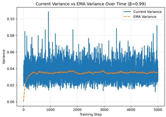
To explicitly analyze the stability of the EMA-based variance normalization in G-SNR, we connect the empirical measurements to the theoretical behavior described in Section 3.3 (Equation (5)–(7)). Specifically, we log: (i) the instantaneous batch-mean variance statistic in Equation (5) as cur_var, (ii) the EMA baseline as ema_var, and (iii) the resulting residual gate values in Equation (10) as gate. We verify three properties: (1) batch-wise smoothing: Equation (6) implies that high-frequency fluctuations in cur_var should be attenuated by EMA; (2) β-dependent stability: Equation (7) predicts that the estimator variance decreases as increases; and (3) layer-wise consistency and gating stability: a more stable baseline should yield more consistent reliability gates across layers.
Table 11 summarizes the mean and standard deviation of cur_var, ema_var, and gate under different EMA decays . While the means are nearly unchanged across , the dispersion of the EMA baseline (ema_var std) decreases as increases (from 0.040460 at to 0.040296 at ), which is consistent with the variance suppression trend implied by Equation (7). Moreover, the discrepancy monotonically decreases as increases, indicating a more consistent normalization baseline with slower EMA updates. In particular, the smallest discrepancy is achieved by (), followed by (), (), and ().
Table 11.
Stability statistics of variance normalization and gate activations under different EMA decays . We report the mean and standard deviation over training iterations (steps/batches) for the instantaneous batch statistic (cur_var), EMA baseline (ema_var), and the residual gate activation (gate).
- Batch-wise stability (temporal smoothing).
Figure 6 visualizes the temporal evolution of cur_var and ema_var during training for . The instantaneous statistic fluctuates substantially due to stochastic mini-batch sampling, while the EMA baseline converges rapidly and remains stable across iterations. This directly supports the smoothing behavior implied by Equation (6).
Figure 6.
Batch-wise stability of EMA variance normalization (). The instantaneous statistic (cur_var) fluctuates strongly due to mini-batch randomness, whereas the EMA baseline (ema_var) converges smoothly and remains stable across training iterations.
- Layer-wise consistency.
Beyond temporal stability, we further examine whether the EMA baseline behaves consistently across network depth. Figure 7 shows the evolution of layer-wise EMA variance under different values. Larger leads to smoother and more coherent layer-wise profiles, whereas smaller introduces noisier behavior across layers. This indicates that increasing stabilizes the baseline across depth, consistent with the variance suppression trend in Equation (7).
Figure 7.
Layer-wise consistency of EMA variance under different . Higher produces smoother and more consistent EMA baselines across layers, whereas smaller introduces higher temporal/layer-wise noise.
- Stability of reliability gating.
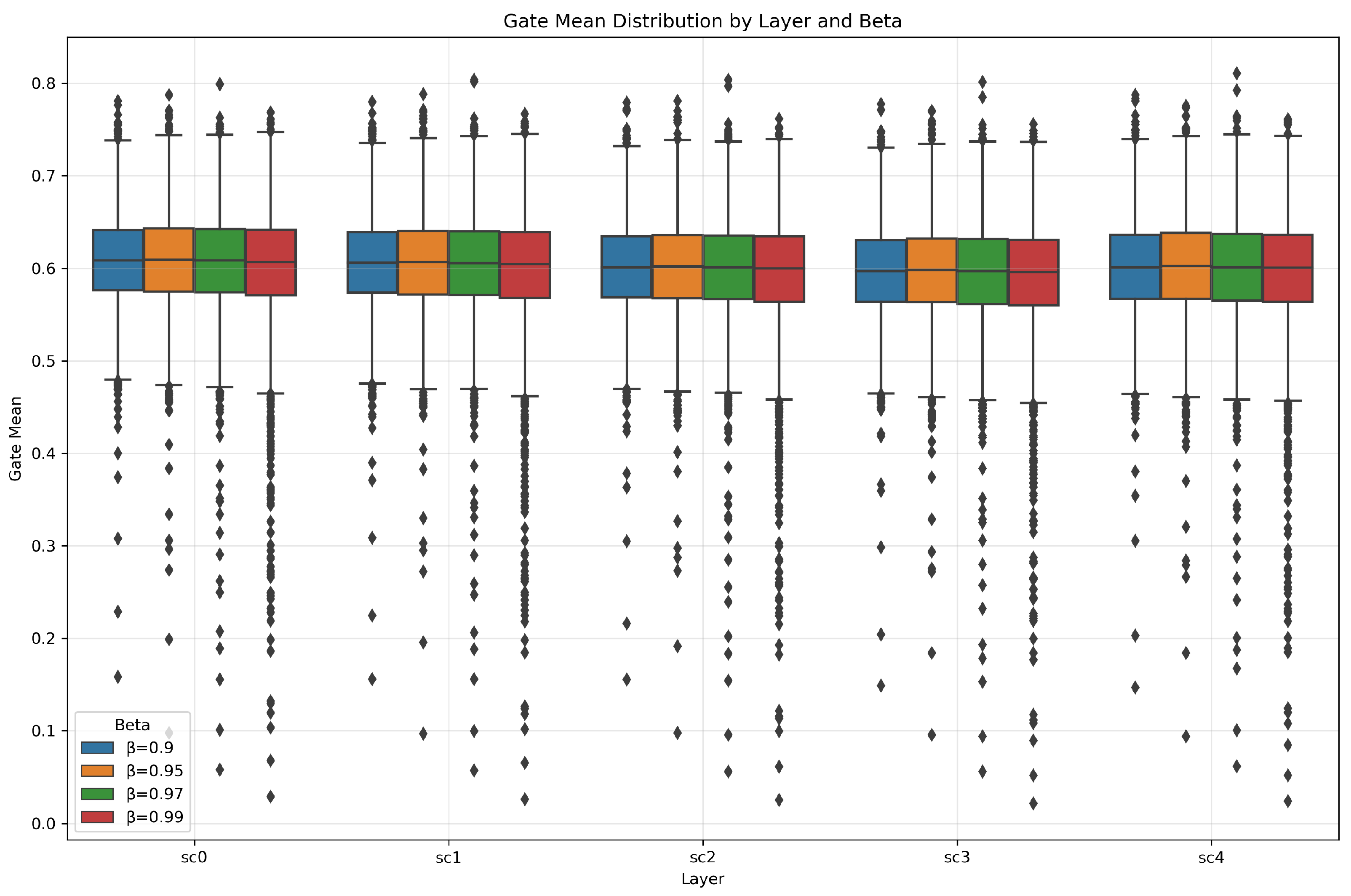
Finally, Figure 8 visualizes the distribution of the residual G-SNR gate values (Equation (10)) across layers for different . The gate values remain well-centered without collapsing to extreme values, indicating well-behaved reliability modulation. Larger yields tighter distributions with fewer outliers, suggesting that improved baseline stability translates into more consistent reliability scores across both batches and layers.
Figure 8.
Distribution of G-SNR gate activations across layers under different . Higher yields more concentrated gate distributions with fewer extreme responses, indicating more stable reliability estimation across layers.
For completeness, we further provide a formal convergence analysis of the EMA-based variance estimator in Appendix A, where we derive a closed-form bound on the asymptotic variance and theoretically justify the stabilizing effect of larger .
4.5.4. Effect of Neighborhood Size k
Finally, we examine the influence of the neighborhood size k in the backbone. Consistent with the analysis in Section 4.4, AGSM-CPA is not critically sensitive to k within the standard range used by RISurConv (). Aggressively reducing k leads to unstable local statistics and severely degraded performance, while moderately increasing k provides no consistent improvement. These observations confirm that AGSM-CPA does not rely on specialized neighborhood configurations and integrates naturally with standard backbone settings.
Overall, these ablation studies demonstrate that the robustness gains of AGSM-CPA are driven by principled architectural design rather than careful hyperparameter tuning. The consistent contributions of G-SNR and CP-SCL, together with their stability across reasonable parameter ranges, support our central claim: explicitly modeling local geometric reliability and enforcing cross-perturbation consistency provides a practical and effective path toward robust, rotation-invariant point cloud recognition.
4.6. Part Segmentation on ShapeNetPart
Finally, we examine whether the robustness learned in classification transfers to fine-grained part segmentation. We plug AGSM-CPA into the RISurConv segmentation backbone and evaluate on ShapeNetPart. Following common practice, we report per-category mIoU on clean inputs and under Gaussian noise with applied at test time (without retraining). Results are summarized in Table 12.
Table 12.
Part segmentation mIoU on ShapeNetPart under clean and noisy inputs ().
AGSM-CPA achieves competitive mIoU on most common categories (e.g., Mug, Chair, Guitar). Highly articulated or thin-structured objects (e.g., Rocket, Earphone, Motorbike) remain more challenging, where small geometric perturbations may alter part boundaries and local topology.
Under moderate Gaussian noise (), performance drops only slightly for most categories, indicating good stability of per-point predictions. We also observe that the noisy mIoU of Motorbike slightly increases (0.503→0.514), which we attribute to mild noise acting as a regularizer on ambiguous shapes; nevertheless, the overall trend remains that noise leads to small accuracy degradation. These results suggest that the reliability signal learned by G-SNR is not limited to global classification, but can also support robust local decisions in segmentation.
4.7. Qualitative Results and Failure Analysis
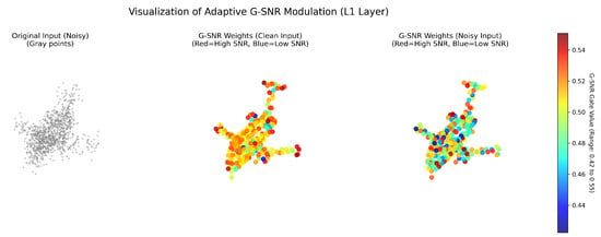
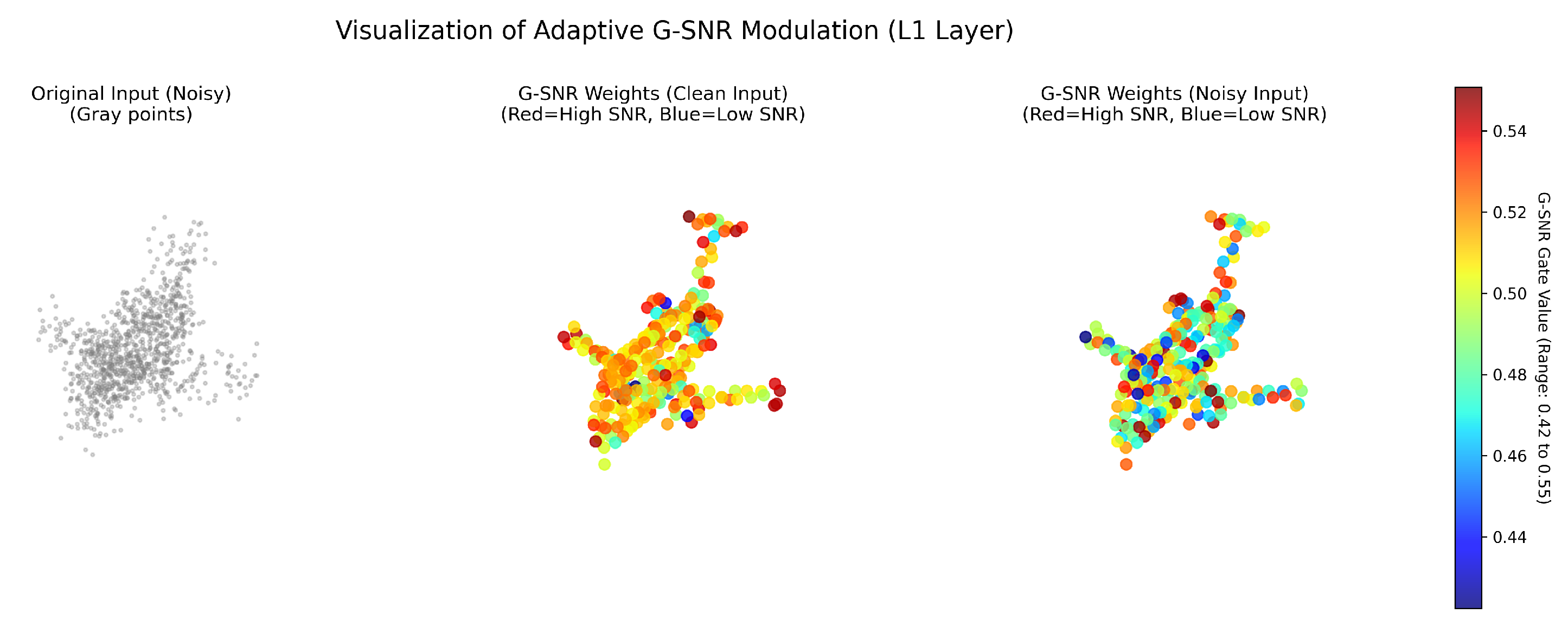
We provide qualitative evidence of how G-SNR responds to geometric corruption. Figure 9 visualizes the predicted G-SNR weights at shallow layers. Intuitively, regions that are sparse, irregular, or strongly perturbed tend to receive lower weights, while stable surfaces keep higher confidence.
Figure 9.
Visualization of G-SNR behavior under clean and noisy inputs. (Left): the noisy input point cloud (gray) as reference. (Middle): G-SNR weights predicted from the clean input. (Right): G-SNR weights predicted from the noisy input, where corrupted regions are down-weighted (blue).
As shown in Figure 9, G-SNR produces a spatially structured reliability map: low-weight regions often coincide with locally unstable geometry (e.g., perturbed or isolated points), reducing their influence on subsequent feature aggregation. In contrast, stable surface regions preserve higher weights, which helps the model retain consistent cues for recognition.
- Failure cases.
AGSM-CPA is not immune to extreme degradation. When the input becomes extremely sparse (e.g., very few points) or large portions of the shape are missing (e.g., severe occlusion), both the baseline and our method may fail due to insufficient geometric evidence. In such cases, we observe that AGSM-CPA tends to produce less overconfident predictions than the baseline, consistent with its explicit suppression of unreliable neighborhoods.
5. Conclusions
We proposed AGSM-CPA, a lightweight add-on framework that improves the robustness of rotation-invariant point cloud networks under realistic geometric imperfections. Our key observation is that formal rotation invariance does not guarantee numerical stability: when local neighborhoods become unreliable due to noise, occlusion, or irregular sampling, early-layer features can be ill-conditioned and degrade the downstream prediction.
To address this, AGSM-CPA introduces two simple mechanisms: (i) G-SNR, which estimates local geometric reliability from rotation-invariant statistics and modulates features accordingly; and (ii) CP-SCL, which enforces prediction consistency between weakly and strongly corrupted views during training. Both components preserve the rotation-invariant structure of the backbone and add negligible computational overhead at inference.
Experiments on ModelNet40 and ScanObjectNN demonstrate that AGSM-CPA improves clean accuracy while providing substantial gains under common corruptions such as noise and point dropout. We further verify transferability on ShapeNetPart, where mIoU degrades only mildly under test-time noise, suggesting that the learned reliability signal is useful for fine-grained per-point decisions. Qualitative visualizations confirm that G-SNR adaptively down-weights geometrically unstable regions, which aligns with the intended design.
Our current reliability estimate relies on simple neighborhood statistics and may not fully capture complex sensing artifacts or structured occlusions. In particular, we primarily target rigid-motion-preserving corruptions (e.g., noise, dropout, and block erasing), and do not explicitly model non-rigid deformations that may occur in articulated objects or dynamic scans. Future work includes incorporating richer geometric cues (e.g., density changes or surface smoothness), designing perturbations that better match real acquisition processes, extending the framework to non-rigid or time-varying point clouds, and scaling to larger tasks such as detection or scene understanding.
Author Contributions
Conceptualization, M.G.; methodology, M.G.; software, M.G.; validation, M.G. and S.W.; formal analysis, M.G.; investigation, M.G.; resources, M.G.; data curation, M.G.; writing—original draft preparation, M.G.; writing—review and editing, M.G., Y.Y. and J.Y.; visualization, M.G.; supervision, Y.Y. and J.Y.; project administration, J.Y. All authors have read and agreed to the published version of the manuscript.
Funding
This work was supported by the National Natural Science Foundation of China (No. 62072388), the Fujian Provincial Science and Technology Major Project (No. 2024HZ022003), the Jiangxi Provincial Natural Science Foundation Key Project (No. 20244BAB28039), the Xiamen Public Technology Service Platform (No. 3502Z20231043), and the Fujian Sunshine Charity Public Welfare Foundation. The APC was funded by the authors.
Data Availability Statement
The datasets used in this study are publicly available: ModelNet40 (https://modelnet.cs.princeton.edu/, accessed on 12 October 2025), ScanObjectNN (https://hkust-vgd.github.io/scanobjectnn/, accessed on 12 October 2025), and ShapeNetPart (https://shapenet.org/, accessed on 12 October 2025). No new data were generated in this work.
Acknowledgments
The authors would like to thank Xiamen University for providing computational resources and technical support that made this work possible.
Conflicts of Interest
The authors declare no conflicts of interest.
Appendix A. Stability Analysis of EMA Normalization
This appendix provides the theoretical analysis supporting the empirical observations reported in Section 4.5.3. In particular, we analyze the convergence behavior of the EMA-based variance estimator used in G-SNR and derive a closed-form bound on its variance.
Proposition A1
(Convergence of EMA variance). Let denote the observed batch-mean variance at optimization step t for a fixed layer ℓ. Assume that the sequence is (approximately) stationary with constant variance and negligible cross-batch correlation. Consider the EMA update (Equation (5))
with and fixed initialization . Then the variance of the estimator converges to
Proof.
For notational simplicity, we omit the layer index and write , . The EMA update is
Unrolling the recurrence yields
Since is constant and has constant variance with negligible cross-batch correlation, we have
The sum is a geometric series with ratio , hence
Taking gives
Reintroducing the layer index completes the proof. □
The proposition shows that EMA significantly suppresses the variance induced by mini-batch sampling. For the default , the reduction factor is
so the variance of the EMA baseline is only about of the raw batch variance. Consequently, the normalized quantities (Equation (8)) and the resulting G-SNR reliability scores (Equation (9)) remain highly stable across training iterations.
References
- Li, H. RWAFormer: A lightweight road LiDAR point cloud segmentation network based on transformer. ISPRS Open J. Photogramm. Remote Sens. 2024, 12, 100063. [Google Scholar] [CrossRef] [Scilit]
- Zhu, S.; Li, Q.; Zhao, J.; Zhang, C.; Zhao, G.; Li, L.; Chen, Z.; Chen, Y. A Deep-Learning-Based Method for Extracting an Arbitrary Number of Individual Power Lines from UAV-Mounted Laser Scanning Point Clouds. Remote Sens. 2024, 16, 393. [Google Scholar] [CrossRef] [Scilit]
- Guo, Y.; Wang, H.; Hu, Q.; Liu, J.; Liu, L.; Bennamoun, M. Deep Learning for 3D Point Clouds: A Survey. IEEE Trans. Pattern Anal. Mach. Intell. 2021, 43, 4338–4364. [Google Scholar] [CrossRef] [Scilit] [PubMed]
- Qi, C.R.; Su, H.; Mo, K.; Guibas, L.J. PointNet: Deep Learning on Point Sets for 3D Classification and Segmentation. In Proceedings of the IEEE Conference on Computer Vision and Pattern Recognition (CVPR), Honolulu, HI, USA, 21–26 July 2017; pp. 652–660. [Google Scholar]
- Qi, C.R.; Yi, L.; Su, H.; Guibas, L.J. PointNet++: Deep Hierarchical Feature Learning on Point Sets in a Metric Space. In Proceedings of the Advances in Neural Information Processing Systems (NeurIPS), Long Beach, CA, USA, 4–9 December 2017. [Google Scholar]
- Wang, Y.; Sun, Y.; Liu, Z.; Sarma, S.E.; Bronstein, M.M.; Solomon, J.M. Dynamic Graph CNN for Learning on Point Clouds. ACM Trans. Graph. 2019, 38, 1–12. [Google Scholar] [CrossRef] [Scilit]
- Thomas, H.; Qi, C.R.; Deschaud, J.E.; Marcotegui, B.; Goulette, F.; Guibas, L.J. KPConv: Flexible and Deformable Convolution for Point Clouds. In Proceedings of the IEEE/CVF International Conference on Computer Vision (ICCV), Seoul, Republic of Korea, 27 October–2 November 2019; pp. 6411–6420. [Google Scholar]
- Guo, M.H.; Cai, T.X.; Liu, Z.N.; Mu, T.; Martin, R.; Hu, S.M.; Lee, T.Y. PCT: Point Cloud Transformer. Comput. Graph. 2021, 99, 92–102. [Google Scholar] [CrossRef] [Scilit]
- Wu, X.; Jiang, L.; Wang, P.S. Point Transformer V3: Simpler, Faster, Stronger. In Proceedings of the IEEE/CVF Conference on Computer Vision and Pattern Recognition (CVPR), Seattle, WA, USA, 16–22 June 2024. [Google Scholar]
- Liang, D.; Zhou, X.; Wang, W. Point-Mamba: A Simple State Space Model for Point Cloud Analysis. arXiv 2024, arXiv:2402.10739. [Google Scholar]
- Wu, Z.; Song, S.; Khosla, A.; Yu, F.; Zhang, L.; Tang, X.; Xiao, J. 3D ShapeNets: A Deep Representation for Volumetric Shapes. In Proceedings of the IEEE Conference on Computer Vision and Pattern Recognition (CVPR), Boston, MA, USA, 7–12 June 2015; pp. 1912–1920. [Google Scholar]
- Rao, Y.; Lu, J.; Zhou, J. Spherical Fractal Convolutional Neural Networks for Point Cloud Recognition. In Proceedings of the IEEE/CVF Conference on Computer Vision and Pattern Recognition (CVPR), Long Beach, CA, USA, 15–20 June 2019. [Google Scholar]
- Poulenard, A.; Rakotosaona, M.J.; Ponty, Y.; Ovsjanikov, M. Effective Rotation-Invariant Point CNN with Spherical Harmonics Kernels. In Proceedings of the International Conference on 3D Vision (3DV), Québec City, QC, Canada, 16–19 September 2019. [Google Scholar]
- Zhang, Z.; Hua, B.S.; Rosen, D.W.; Yeung, S.K. Rotation Invariant Convolutions for 3D Point Clouds Deep Learning. In Proceedings of the International Conference on 3D Vision (3DV), Québec City, QC, Canada, 16–19 September 2019. [Google Scholar]
- Zhang, Z.; Hua, B.S.; Yeung, S.K. RIConv++: Effective Rotation-Invariant Convolutions for 3D Point Clouds. arXiv 2022, arXiv:2202.13094. [Google Scholar]
- Lou, Y.; Ye, Z.; You, Y.; Jiang, N.; Lu, J.; Wang, W.; Ma, L.; Lu, C. CRIN: Centrifugal Reference Frame for Rotation-Invariant Point Cloud Analysis. In Proceedings of the AAAI Conference on Artificial Intelligence (AAAI), Washington, DC, USA, 7–14 February 2023; Volume 37, pp. 1847–1855. [Google Scholar]
- Zhang, Z.; Yang, L.; Xiang, Z. RISurConv: Rotation Invariant Surface Attention-Augmented Convolutions for 3D Point Cloud Classification and Segmentation. arXiv 2024, arXiv:2408.06110. [Google Scholar]
- Pang, Y. RI-MAE: Rotation-Invariant Masked AutoEncoders for Self-Supervised Point Cloud Representation Learning. In Proceedings of the AAAI Conference on Artificial Intelligence (AAAI), Philadelphia, PA, USA, 25 February–4 March 2025. [Google Scholar]
- Uy, M.A.; Pham, Q.H.; Hua, B.S.; Nguyen, D.T.; Yeung, S.K. ScanObjectNN: A Real-World Point Cloud Dataset for Classification. In Proceedings of the IEEE/CVF International Conference on Computer Vision (ICCV), Seoul, Republic of Korea, 27 October–2 November 2019; pp. 1588–1597. [Google Scholar]
- Ye, S.; Chen, Z.; Han, X.; Liao, J. Learning with Noisy Labels for Robust Point Cloud Segmentation. In Proceedings of the IEEE/CVF International Conference on Computer Vision (ICCV), Montreal, QC, Canada, 11–17 October 2021; pp. 6443–6452. [Google Scholar]
- Fei, B.; Yang, W.; Ma, L.; Chen, W.M. DcTr: Noise-robust Point Cloud Completion by Dual-Channel Transformer with Cross-Attention. Pattern Recognit. 2023, 133, 109051. [Google Scholar] [CrossRef] [Scilit]
- She, R.; Kang, Q.; Wang, S.; Tay, W.P.; Zhao, K.; Song, Y. PointDifformer: Robust Point Cloud Registration With Neural Diffusion and Transformer. IEEE Trans. Geosci. Remote Sens. 2024, 62, 5701015. [Google Scholar] [CrossRef] [Scilit]
- Zhao, G.; Guo, Z.; Wang, X.; Ma, H. SphereNet: Learning a Noise-Robust and General Descriptor for Point Cloud Registration. IEEE Trans. Geosci. Remote Sens. 2024, 62, 5700516. [Google Scholar] [CrossRef] [Scilit]
- Li, X.; Lu, J.; Ding, H.; Sun, C.; Zhou, J.T. PointCVaR: Risk-Optimized Outlier Removal for Robust 3D Point Cloud Classification. In Proceedings of the AAAI Conference on Artificial Intelligence (AAAI), Vancouver, BC, Canada, 20–27 February 2024. [Google Scholar]
- Huang, Y.; Zhang, M.; Ding, D. CausalPC: Improving the Robustness of Point Cloud Classification by Causal Effect Identification. In Proceedings of the IEEE/CVF Conference on Computer Vision and Pattern Recognition (CVPR), Seattle, WA, USA, 16–22 June 2024. [Google Scholar]
- Hoppe, H.; DeRose, T.; Duchamp, T.; McDonald, J.; Stuetzle, W. Surface Reconstruction from Unorganized Points. In Proceedings of the 19th Annual Conference on Computer Graphics and Interactive Techniques (SIGGRAPH), Chicago, IL, USA, 27–31 July 1992; pp. 71–78. [Google Scholar] [CrossRef] [Scilit]
- Mitra, N.J.; Nguyen, A. Estimating Surface Normals in Noisy Point Cloud Data. In Proceedings of the Nineteenth Annual Symposium on Computational Geometry, San Diego, CA, USA, 8–10 June 2003; pp. 322–328. [Google Scholar]
- Digne, J.; de Franchis, C. The Bilateral Filter for Point Clouds. Image Process. Line 2017, 7, 278–287. [Google Scholar] [CrossRef] [Scilit]
- Guerrero, P.; Kleiman, Y.; Ovsjanikov, M.; Mitra, N.J. PCPNet: Learning Local Shape Properties from Raw Point Clouds. Comput. Graph. Forum 2018, 37, 75–85. [Google Scholar] [CrossRef] [Scilit]
- Tarvainen, A.; Valpola, H. Mean Teachers Are Better Role Models: Weight-Averaged Consistency Targets Improve Semi-Supervised Deep Learning Results. In Proceedings of the Advances in Neural Information Processing Systems, Long Beach, CA, USA, 4–9 December 2017. [Google Scholar]
- Xie, Q.; Dai, Z.; Hovy, E.; Luong, M.T.; Le, Q.V. Unsupervised Data Augmentation for Consistency Training. In Proceedings of the Advances in Neural Information Processing Systems, Virtual, 6–12 December 2020. [Google Scholar]
- Berthelot, D.; Carlini, N.; Cubuk, E.D.; Kurakin, A.; Sohn, K.; Zhang, H.; Raffel, C. MixMatch: A Holistic Approach to Semi-Supervised Learning. In Proceedings of the Advances in Neural Information Processing Systems, Vancouver, BC, Canada, 8–14 December 2019. [Google Scholar]
- Zhao, H.; Jiang, L.; Jia, J.; Torr, P.; Koltun, V. Point Transformer. In Proceedings of the IEEE/CVF International Conference on Computer Vision (ICCV), Montreal, QC, Canada, 10–17 October 2021; pp. 16259–16268. [Google Scholar]
- Yu, X.; Tang, L.; Rao, Y.; Huang, T.; Zhou, J.; Lu, J. Point-BERT: Pre-Training 3D Point Cloud Transformers with Masked Point Modeling. In Proceedings of the IEEE/CVF Conference on Computer Vision and Pattern Recognition (CVPR), New Orleans, LA, USA, 18–24 June 2022. [Google Scholar]
- Yu, H.; Qin, Z.; Hou, J.; Saleh, M.; Li, D.; Busam, B.; Ilic, S. Rotation-Invariant Transformer for Point Cloud Matching. In Proceedings of the IEEE/CVF Conference on Computer Vision and Pattern Recognition (CVPR), Vancouver, BC, Canada, 18–22 June 2023. [Google Scholar]
- Qin, C.; Hou, S.; Pang, M.; Wang, Z.; Zhang, D. Reinforcement learning-based secure tracking control for nonlinear interconnected systems: An event-triggered solution approach. Eng. Appl. Artif. Intell. 2025, 161, 112243. [Google Scholar] [CrossRef] [Scilit]
- Zhang, D.; Yuan, Q.; Meng, L.; Xia, R.; Liu, W.; Qin, C. Reinforcement learning for single-agent to multi-agent systems: From basic theory to industrial application progress, a survey. Artif. Intell. Rev. 2025, 59, 46. [Google Scholar] [CrossRef] [Scilit]
- Qin, C.; Pang, M.; Wang, Z.; Hou, S.; Zhang, D. Observer-Based Fault-Tolerant Control Design for Saturated Nonlinear Systems with Full State Constraints via a Novel Event-Triggered Mechanism. Eng. Appl. Artif. Intell. 2025, 161, 112221. [Google Scholar] [CrossRef] [Scilit]
- Yi, L.; Kim, V.; Ceylan, D.; Shen, I.; Su, H.; Lu, C.; Huang, Q.; Guibas, L.J. A Scalable Active Framework for Region Annotation in 3D Shape Collections. In Proceedings of the ACM SIGGRAPH Asia, Macao, China, 5–8 December 2016. [Google Scholar]
- Qian, G.; Li, Y.; Peng, H.; Mai, J.; Hammoud, H.; Elhoseiny, M.; Ghanem, B. PointNeXt: Revisiting PointNet++ with Improved Training and Scaling Strategies. In Proceedings of the Advances in Neural Information Processing Systems (NeurIPS), New Orleans, LA, USA, 10–16 December 2022. [Google Scholar]



Disclaimer/Publisher’s Note: The statements, opinions and data contained in all publications are solely those of the individual author(s) and contributor(s) and not of MDPI and/or the editor(s). MDPI and/or the editor(s) disclaim responsibility for any injury to people or property resulting from any ideas, methods, instructions or products referred to in the content. |
© 2026 by the authors. Licensee MDPI, Basel, Switzerland. This article is an open access article distributed under the terms and conditions of the Creative Commons Attribution (CC BY) license.