Classifying Consensus Sequences Using Point-Set Representations

Abstract

Consensus sequences at sites such as exon–intron boundaries or branch points are displayed with sequence logos. Implicit in this representation is a presumption of independence of nucleic acids at distinct sites; consequently, sequence logos fail to elicit higher-order statistical characteristics within nucleic acid sequences. We introduce a graphical approach to display such features. Probability distribution functions on these point-sets are used to highlight correlations at exon–intron boundaries and at branch points. Point-sets provide a more intuitive view of the differences than quantitative tests like the Kolmogorov–Smirnov test. Differences in density functions at normal exon–exon boundaries and cancer fusion junctions can be used to highlight the distinctions between the two classes of junctions. The fractal structure of point-sets for sites within exons and within introns emerges as the neighborhood used for its construction is enlarged. The two sets can be differentiated using their singularity spectra.

1. Motivation and Introduction

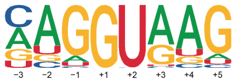
Our genome consists of two three-billion-long, pairwise-linked strands of the nucleic acids guanine (G), cytosine (C), adenine (A), and thymine (T), anchored by two sugar-phosphate backbones. In stable states, all complementary nucleic acid pairs between the two strands are Watson–Crick pairs G-C or A-T [1], although there can be transient non-Watson–Crick pairings. When pre-messenger RNAs (pre-mRNAs) are transcribed from the genome, thymine is replaced by uracil (U). Unlike in the genome, pairings between nucleic acids in RNA strings are non-unique [2]. This variability may originate from smaller energy differentials between pairs of nucleic acids in RNA than those in DNA, as found in ab initio quantum mechanical calculations [3,4,5,6,7,8,9,10]. The most likely collection of sub-sequences near a site of interest are known as consensus sequences and are displayed using sequence logos [11,12,13,14], such as that shown in Figure 1, which describes a boundary of interest for splicing. The site immediately to the right of the boundary ($+1$ site) is always a G, while the next ($+2$) is a U in over 99% of cases. However, the remaining sites in the neighborhood are not unique. Sequence logos presuppose independence between nucleic acids at distinct binding sites; consequently, they fail to elucidate facets such as correlations between neighboring sites or between short neighboring sequences. This paper introduces an approach that aids in visualizing such higher-order statistics and other structural properties of sub-sequences.

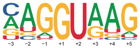
Figure 1. A sequence logo representing the probability of finding nucleic acids at sites neighboring an exon–intron boundary. The two left-most sites within the intron are nearly always $GU$. The likelihood at other sites is proportional to the heights of the symbols. The four colors are used to distinguish nucleic acid symbols.

Shortly after transcription, pre-mRNAs are spliced through a complex series of actions carried out in a ∼20 nm RNA–protein complex, known as the spliceosome [15,16,17,18,19]. Segments of non-coding RNA that are spliced out are referred to as introns, while those that are retained are called exons [15,20,21,22,23,24,25]. Typically, consecutive exons are fused to form messenger RNA (mRNA)—although sometimes exons are bypassed, yielding alternatively spliced mRNA [26,27,28,29]. In addition, occasionally, transcripts from different genes ligate via trans-splicing [30,31,32,33,34,35]. Some alternatively spliced and trans-spliced mRNAs are translated to proteins as well [26], thus enriching the proteome [36].

Parts of the machinery used in splicing are the small nuclear RNAs (snRNAs) $U1$, $U2$, $U4$, $U5$, and $U6$. $U1$ initiates splicing by binding to an exon–intron boundary, while $U2$ adheres to a downstream site, the branch point, which lies close to the $3^{\prime }$-end of the intron. These two appendages aid in identifying the intronic region to be spliced out. The recognition regions of $U1$ and $U2$, which play a crucial role in binding the pre-mRNA, are only ∼10 nucleotides long [37].

Unfortunately, sequence logos can only furnish frequencies of appearance of nucleic acids at sites of interest; higher-order statistics cannot be elicited from them. A well-known correlation is the compensation effect, which asserts that when the location five sites to the right of the exon–intron boundary (site $+5$) is not occupied by a G, the nucleotide immediately to the left of the boundary (site $-1$) is very likely a G [38,39,40]. Equivalently, if the nucleotide at the $-1$ site is not G, the $+5$ nucleotide is likely to be G. The ability to visualize and quantify such facets of nucleic acid sequences can aid in unraveling the principles underlying preferential selection of consensus sequences.

We introduce a new visual representation of nucleic acid neighborhoods, referred to as point-sets [41], that not only captures the probabilities at nucleic acid sites but also permits intuitive visualization of correlations between neighboring sites or sub-sequences. As applications, we highlight features that emerge from point-set representations at exon–intron boundaries and at branch points. In addition, we argue that point-sets of nucleic acid sequences within exons and within introns are fractals, and we show that fractal measures can be used to discern them. Furthermore, we use point-sets to highlight differences between normal exon–exon boundaries and cancer fusion junctions.

2. Point-Set Representation

Consider a $(2M+1)$-long segment of a genomic sequence ${\left\{S_n\right\}}_{n=-M}^M$, where $S_k$s are nucleic acids A, C, G, or U, and M is sufficiently large. We search for properties in the neighborhood of $S_1$ (we do not have $S_0$ in the sequence, for consistency with the notation used for sequence logos). The representation introduced below is predicated on the assumption that sites closer to $S_1$ play a more significant role in its fate, e.g., if it becomes an exon–intron boundary or a branch point. As an example, suppose we wish to characterize the nature of the neighborhood of the $GU$ dyad (hereafter expressed as $\left|GU\right|$) at the exon–intron boundary. Begin by assigning the integers $\{0,1,2,3\}$ to $\{A,G,U,C\}$ [41]. We can search N-long sub-sequences ($N+1\le M$) to the right (anterior) and to the left (posterior) of $\left|GU\right|$. The sub-sequences can be uniquely represented through a pair of numbers defined through quaternary expansions:

$$x={\displaystyle \sum _{i=1}^N}{\displaystyle \frac{1}{4^i}}{S}_{2+i};y={\displaystyle \sum _{i=1}^N}{\displaystyle \frac{1}{4^i}}{S}_{-i}.$$

(1)

Coordinates x and y bear a one-to-one relationship to the (length N) anterior and posterior sub-sequences of $\left|GU\right|$, with more proximal sites contributing a higher weight. For example, the sub-string $\dots GAC\left|GU\right|ACG\dots$ has coordinates $x={\displaystyle \frac{0}{4}}+{\displaystyle \frac{3}{16}}+{\displaystyle \frac{1}{64}}=0.203125;y={\displaystyle \frac{3}{4}}+{\displaystyle \frac{0}{16}}+{\displaystyle \frac{1}{64}}=0.765625$ (note that the posterior sequence is read backwards). The set of points $(x,y)$ for a collection of exon–intron boundaries is the associated point-set. Point-sets and kneading transformations that map a site to its successor were introduced in Ref. [41]. Here, we focus on probability density functions $\rho (x,y)$ on point-sets and highlight features that can be inferred.

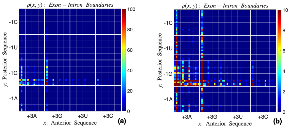
Equation (1) implies that $0\le x,y<1$. Figure 2 shows the probability density function of the point-set at exon–intron junctions in $[0,1]\times [0,1]$. With $N=3$, the domain is partitioned into $64\times 64$ squares. To aid with visualization, the x and y ranges are partitioned into quartiles by thick white lines. The four quartiles in the x direction correspond to sub-sequences with $S_3=0,1,2,\mathrm{and}3$, i.e., sub-sequences with $+3A$, $+3G$, $+3U$, and $+3C$, respectively. Each quartile, partitioned into sub-quartiles by thinner lines, corresponds to $+4A$, $+4G$, $+4U$, and $+4C$. These, in turn, are quartered according to the nucleic acid at the $+5$ site. Corresponding partitioning of the y axis yields primary quartiles $-1A$, $-1G$, $-1U$, and $-1C$, as well as sub-partitions defined by nucleic acids at sites $-2$ and $-3$. Note that we can increase $M_R$ and $M_L$ if a longer neighborhood of the $5^{\prime }$s needs to be analyzed. However, this will decrease the size of individual sectors; for example, if $N=4$, the unit square will be partitioned into $256\times 256$ blocks.

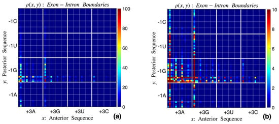
Figure 2. Probability density function at exon–intron junctions with (a) lower and (b) higher color gradation. The four quarters in the x-axis correspond to $+3A$, $+3G$, $+3U$, and $+3C$. The image on the left shows that the most frequent neighborhoods are $NNG\left|GU\right|AAG$, $NNG\left|GU\right|GAG$, and $CAG\left|GU\right|ANN$, where N can be any nucleotide. The higher-resolution image on the right shows the next most frequent nucleic acid neighborhoods, which include $AAG\left|GU\right|ANN$, $CAG\left|GU\right|GNN$, $NNN\left|GU\right|AAG$, and $NNN|GUGAG$.

Point-sets permit the representation of nucleic acid sequences as collections of points. As illustrated in the examples below, this alternate view of sequences aids us in eliciting previously unsuspected properties. Higher-order statistical features such as correlations and global features such as fractal characteristics within sequences are significantly easier to classify and quantify with point-sets.

2.1. Exon–Intron Junctions

Assignment of an exon–intron boundary is initiated by binding to the recognition region of $U1$ snRNA, whose nucleic acid sequence [40,42] is

$$U1:\dots GUC\left|CA\right|\mathrm{\Psi }\mathrm{\Psi }CAUA\dots ,$$

with $\mathrm{\Psi }$ being a pseudo-uridine, a modified version of U. Up to three nucleic acids to the left of $\left|GU\right|$ and six to its right may be used for binding [43]. Prior to hypothesizing on the rules governing this attachment, it is necessary to classify as many features of consensus sequences as possible. We thus evaluate the probability density function $\rho (x,y)$ of nucleic acid sequences in the immediate neighborhood of known exon–intron junctions.

Sequence data in chromosomes 1–22 was accessed via the ‘refGene’ track of the UCSC Genome Browser using the hg38 genome build (accessed on 19 November 2024) [“http://genome.ucsc.edu (genome hg38)”] [44]. Transcripts without coding sequence boundaries labeled ‘complete’ were discarded. The exon–intron boundaries for each remaining transcript were identified, and 15 nucleotides on each side of the boundaries were retained. Transcripts containing initial and terminal exons with less than 15 nucleotides were excluded from consideration to prevent sampling from intergenic regions. Altogether, there were ∼608,000 junctions, from which 100,000 samples were randomly selected for analysis. Coordinates x and y for each junction were evaluated using Equation (1), and the probability density function was computed, as shown in Figure 2. It should be noted that the density functions of the corresponding neighborhoods of arbitrary $GU$ dyads are significantly different.

Figure 2a shows the probability density in its entire range ∼[0, 100]. Two vertical high-density alleys $NNG\left|GU\right|AAG$ and $NNG\left|GU\right|GAG$, along with a horizontal alley $CAG\left|GU\right|ANN$, can be noted, where N represents any nucleic acid. Figure 2b refines the color range to ∼[0, 10], highlighting the next-most-dense sub-sequences, including $AAG\left|GU\right|ANN$, $CAG\left|GU\right|GNN$, $NNN\left|GU\right|AAG$, and $NNN\left|GU\right|GAG$.

Correlations between neighboring sites of consensus sequences are easily extracted from the point-set representation. For example, when the $-1$ site is not a G (i.e., first, third, and fourth quartiles in the vertical direction), the most frequent anterior sequences are $AAG$ and $GAG$. This not only reinforces the compensation effect (i.e., $+5G$) but also shows that the $+4$ site is primarily A. Similarly, when the $+5$ site is not G (in particular, outside the two dominant vertical alleys), the $-1$ site is almost exclusively G. Note also that the posterior sequences $AAG$ and $CAG$ are more prevalent than others. Furthermore, recent investigations [10,40,45] have proposed that there are two distinct classes of junction neighborhoods—one of type $NN\left|GU\right|RAG$ and the other $AG\left|GU\right|NNN$, where $R\in \{G,A\}$. The two high-density vertical alleys in Figure 2b correspond to the first group, and the horizontal dense region to the second. We reiterate that such subtleties are impossible to deduce from sequence logos.

2.2. Branch Points

The $U2$ snRNA with the recognition region

$$U2:\dots A\mathrm{\Psi }GA\mathrm{\Psi }GUG\dots$$

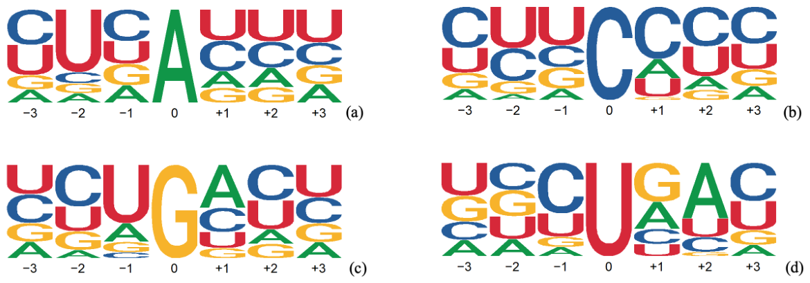
is used to select a branch point that precedes the polypyrimidine tract and sits ∼18–38 nucleotides from the end of the intron [46]. Its binding initiates a complex series of actions by several protein complexes to discard the intron. The branch point itself is not unique, being A in 79%, C in 9%, G in 4%, and U in 8% of the ∼56,000 unique experimental samples given in Ref. [47]. The sequence logos for the four cases differ significantly, as shown in Figure 3.

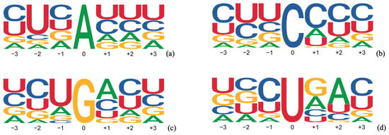
Figure 3. Sequence logos at neighborhoods of the branch point (a) when the branch point is A, (b) when the branch point is C, (c) when the branch point is G, and (d) when the branch point is U.

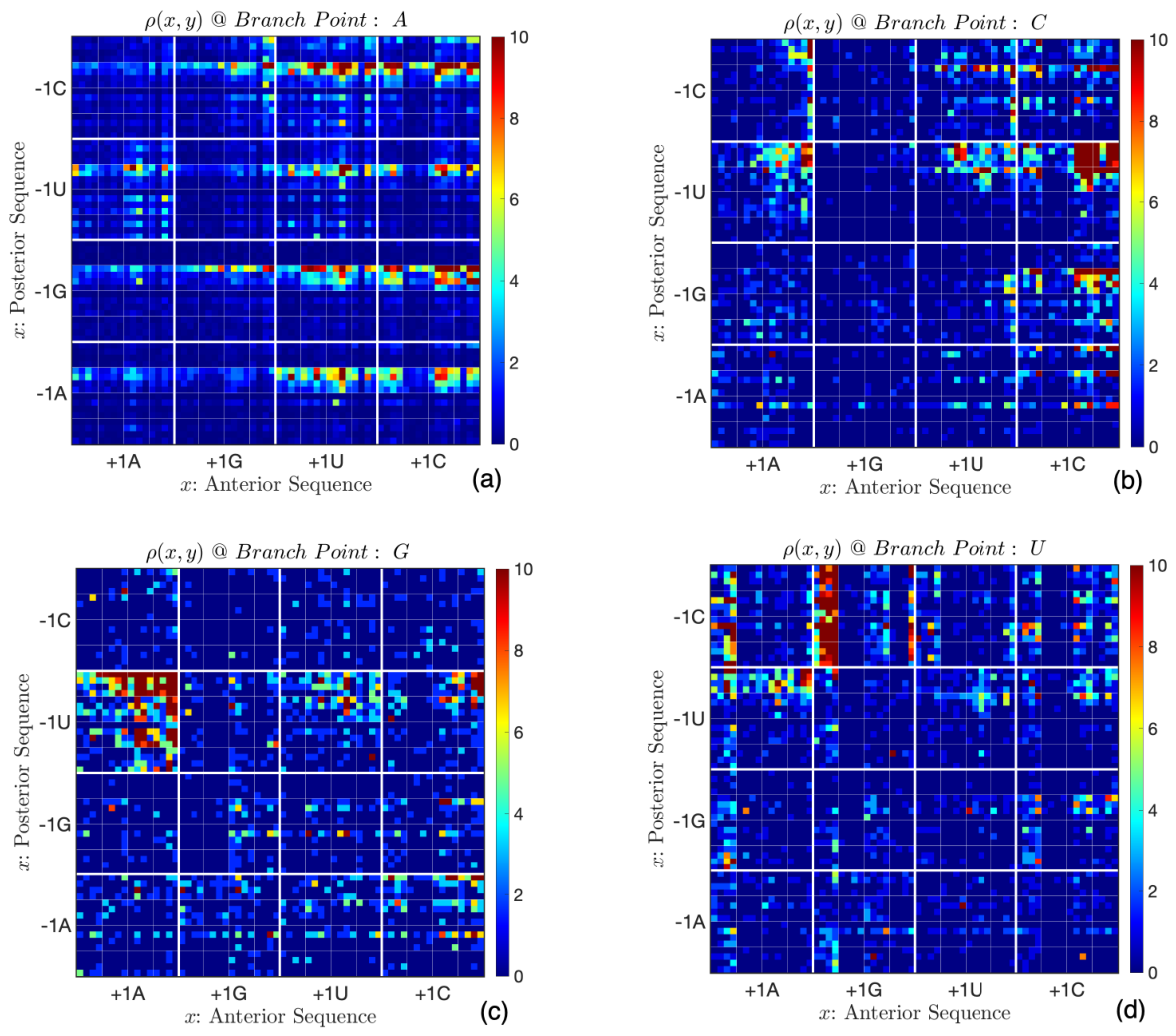
Figure 4 shows the probability density functions on point-sets for the four cases. Since the branch point is defined with a single nucleotide (in place of $\left|GU\right|$ for an exon–intron boundary), the computation of x starts with the site immediately to the right of the branch point, with appropriate modification of Equation (1). With a branch point A, the consensus sequences are $CUN\left|A\right|UNN$ and $CUN\left|A\right|CNN$, while the sequences $NCU\left|C\right|CCN$ and $NCU\left|C\right|CUN$ dominate when the branch point is C. The sequences $NCU\left|G\right|ANN$ (resp. $NNC\left|U\right|GAN$) are most frequent when the branch point is G (resp. U). Correlations are also manifest. In Figure 4a, the anterior sequences are primarily of type $ACU$ or $AUU$ when the $-2$ site is not U (i.e., outside the horizontal lines). When the branch point is U, i.e., Figure 4d, the $-1$ site is dominantly C when the first two posterior sites are $GA$ or $AA$, or when the first three sites are $GCC$.

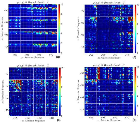
Figure 4. Consensus sequences depend on the nucleic acid at the branch point. (a) When it is A, the most frequent consensus sequences are $CUN\left|A\right|UNN$ and $CUN\left|A\right|CNN$. (b) With C as the branch point, the primary consensus sequences take the forms $NCU\left|C\right|CCN$ and $NCU\left|C\right|CUN$. (c) With G as the branch point, they take the form $NCU\left|G\right|ANN$, while (d) if it is U, the prevalent form is $NNC\left|U\right|GAN$.

The panels in Figure 4 are visually different. However, the differences depend on the scale; for example, on the scale defined by the first nucleotide on either side (i.e., the domains bounded by thick lines), the densities in Figure 4a–c are close, with the primary difference being in segments defined by $+1G$. However, the density functions are different on a smaller scale. Such assertions can be quantified using a two-dimensional extension of the Kolmogorov–Smirnov test [48]. The statistic d for univariate distributions is the maximum difference between cumulative distribution functions. The significance of the null hypothesis (that the distributions are not different) is independent of the shape of the distribution [48] and in comparing two datasets of N elements each:

$$\mathrm{Prob}\left[d<D\right]=Q_{KS}\left(\sqrt{{\displaystyle \frac{N}{2}}}D\right),$$

(2)

where $Q_{KS}$ is the monotonically decreasing Kolmogorov–Smirnov distribution

$$Q_{KS}\left(\lambda \right)=2{\displaystyle \sum _{j=1}^{\infty }}{(-1)}^{j-1}{e}^{-2j^2{\lambda }^2}.$$

(3)

At a 95% confidence level, the argument of $Q_{KS}$ in Equation (2) is 1.36.

The Kolmogorov–Smirnov test has been extended for comparison of two-dimensional probability distributions [49,50,51]. The cumulative distributions functions are not well defined for this case. It was shown, however, that a good surrogate is the maximum of the integrated probabilities in the four quadrants partitioned by axes running through the point [49]. In order to implement the computation, we divide each point-set into square subdomains (with symmetrically placed bounding rectangles), and we denote the upper-right vertices of the $k^{th}$ square by $(x_k,y_k)$. Following Ref. [51], we then calculate the probabilities $P_{++}\left(k\right)=\mathrm{Prob}[x>x_k;y>y_k]$, $P_{+-}\left(k\right)=\mathrm{Prob}[x>x_k;y<y_k]$, $P_{-+}\left(k\right)=\mathrm{Prob}[x<x_k;y>y_k]$, and $P_{--}\left(k\right)=\mathrm{Prob}[x<x_k;y<y_k]$ for the two point-sets, and we select the largest absolute difference $d_k$ among them. The bivariate Kolmogorov–Smirnov statistic is the maximum among them for all vertices, i.e., $d={\max }_k\left\{d_k\right\}$. Monte-Carlo simulations show that

$$\mathrm{Prob}[d<D]=Q_{KS}\left({\displaystyle \frac{D\sqrt{N/2}}{1+\sqrt{1-r^2}(0.25-0.75\sqrt{2/N})}}\right),$$

(4)

with N being the number of vertices [51]. As in the one-dimensional case, the result is (nearly) independent of the underlying distributions so long as the $x-y$ correlations $r_1$ and $r_2$ of the two distributions are “close.” This condition is valid for most (though not all) of the partitions discussed below. The parameter r is the root-mean-square of $r_1$ and $r_2$.

We compared the pairs of distributions shown in Figure 4 for block sizes of $16\times 16$, $12\times 12$, $10\times 10$, $8\times 8$, $6\times 6$, and $4\times 4$. Figure 4b,c show dissimilarity for block sizes of 12 or smaller, while Figure 4a,b differ only at scales of 6 or smaller. Figure 4a,c differ when the block size is less than 12. Pairwise comparisons of Figure 4a,d, Figure 4b,d, and Figure 4c,d show that they differ at scales smaller than 16. Many of these inferences can be made from visual inspection of Figure 4.

2.3. Normal Exon–Exon Junctions vs. Cancer Fusions

The splicing process terminates when successive exons (or in the case of alternative splicings, an exon and one that is further away) are fused. Errors in alternative or trans-splicing can initiate hereditary diseases like Parkinson’s, neurodegenerative diseases, cystic fibrosis, muscular dystrophy, and some classes of cancer [34,35,46,52,53,54,55,56,57]. Fusing of exons occurs through the binding of anterior and posterior ends to the $U5$ snRNA [45], whose recognition region is [40]

$$U5:\dots \mathrm{\Psi }{C}^{m}A\mathrm{\Psi }UUUCC{G}^{m}C\dots ,$$

where $G^m$ and $C^m$ are methylated forms of guanine and cytosine [58].

Figure 5 shows the sequence logos for junctions with successive exons and cancer-inducing fusion junctions. Although the order of frequencies at sites $-3$, $+2$, and $+3$ differs between the groups, the frequencies themselves are not significantly different. There is little that can be inferred in terms of differences between the two groups from sequence logos.

Figure 5. Sequence logos at (a) normal exon–exon junctions and (b) cancer fusion junctions. Although the order of some frequencies ($-3$, $+2$, and $+3$ sites) has changed, the frequencies themselves are not significantly different.

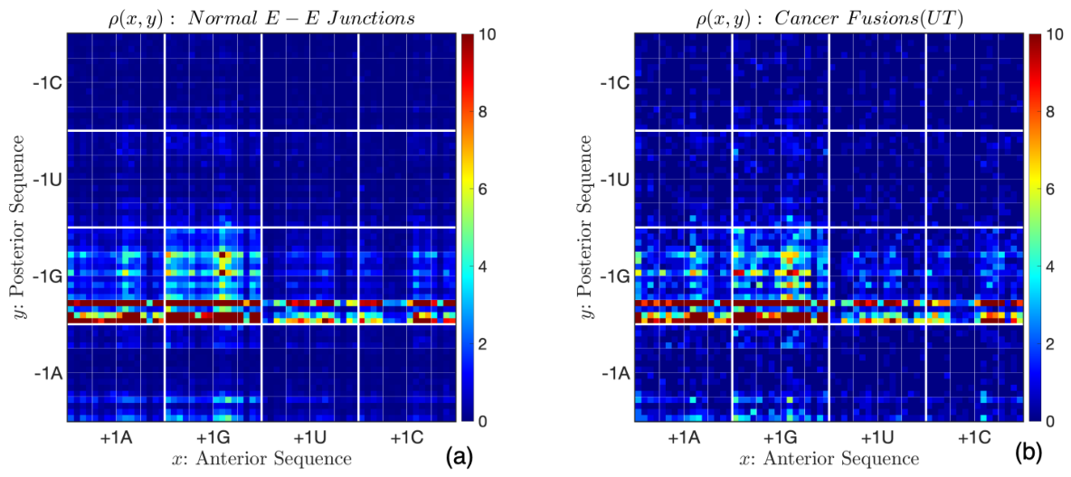
The corresponding point-sets are shown in Figure 6a,b. Once again, they are similar, containing dominant densities of junctions $NAG|NNN$, with the highest densities at $CAG|GNN$, $CAG|ANN$, $AAG|GNN$, and $GAG|GNN$. Point-sets for the exon–exon junctions were derived using the data from the UCSC Genome Browser [http://genome.ucsc.edu (genome hg38)] [44], while those for cancer junctions were extracted from the University of Texas, Houston Fusion Gene Annotation Database (accessed on 22 September 2025) [https://compbio.uth.edu/FusionGDB2/] [59,60,61]. There are ∼11,500 fusion junctions in the database. A similar probability density function was found for fusion junctions from the University of Houston Human Genome Sequencing Center. Neither the two-dimensional Kolmogorov–Smirnov test nor Kullback–Leibler divergence can differentiate between the probability density functions.

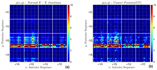
Figure 6. Point-sets at (a) normal exon–exon junctions and (b) cancer fusion junctions. In each case, the dominant forms of the junction are of type $NAG|NNN$, with the highest frequencies of $CAG|ANN$, $CAG|GNN$, $AAG|GNN$, etc.

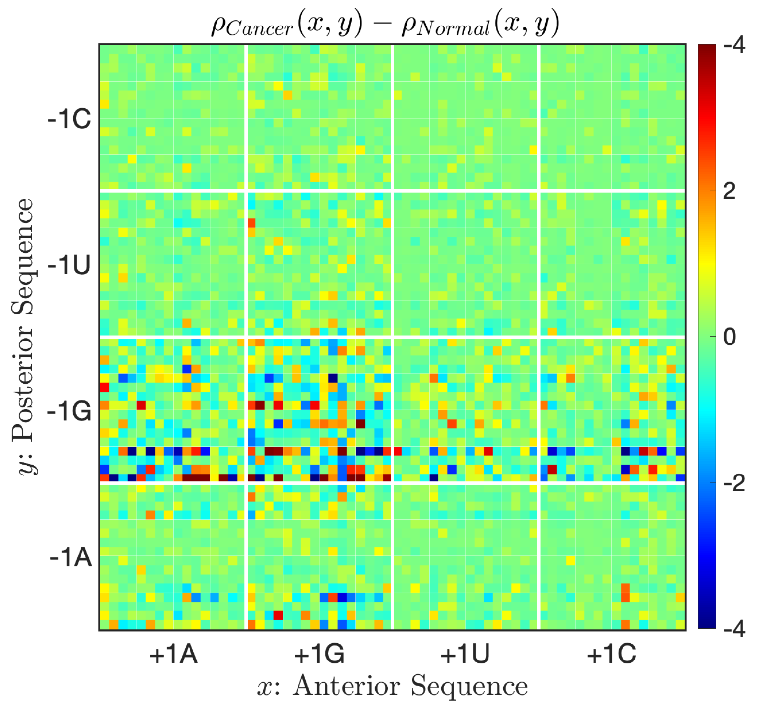
Point-sets permit us to plot differences between the two distribution functions, as shown in Figure 7, which highlights changes prevalent in cancer fusions. Large discords in types $NAG|NNN$ and especially $NAG|GNN$ can be noted. It is difficult to identify such differences using sequence logos or through direct sequence analyses.

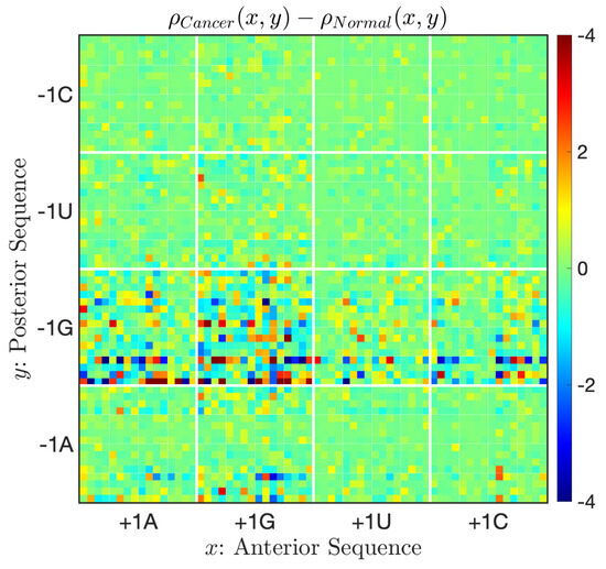
Figure 7. The difference in probability densities between successive exon–exon junctions and cancer fusion junctions. On average posterior sequences, $AAG$ (resp. $CAG$) occurs at a higher (resp. lower) frequency in cancer fusions.

2.4. Fractal Structure of Point-Sets in Sites Within Exons and Within Introns

In this section, we address whether nucleic acid sequences within exons and introns have different characteristics, and if so, how they can be discerned [62]. Exon sequences are highly conserved across species, while non-coding intron sequences can contain mutations and undergo frequent modifications. The density of nucleic acids and dinucleotides differs between sites in introns and in exons.

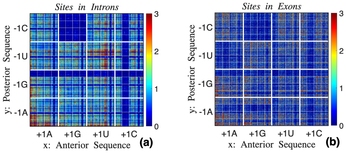
We employed point-sets to search for structural differences between the two groups, since direct analyses of longer sequences is unwieldy. Figure 8 shows point-sets within introns and within exons using $N=5$ long anterior and posterior sequences. The expansion for x starts with $S_0$, while the expansion of y starts with $S_{-1}$. Each set appears to be fractal, an assertion that can be justified as follows: As an example, consider the topmost left block bounded by thick white lines. Points within this domain correspond to sub-sequences of the form $\dots Y_3{Y}_2{Y}_1\left|CC\right|AA|X_1{X}_2{X}_3\dots$, where $X_k$s and $Y_k$s are nucleic acids anterior and posterior to $CC|AA$. Magnifying this subdomain is equivalent to computing points $\dots Y_3{Y}_2{Y}_1|X_1{X}_2{X}_3\dots$, but since the new sub-sequences are within introns as well, the expanded set has similar (not identical) characteristics to the original set. The point-sets of Figure 8 have scale-invariant features, i.e., they are fractal. The low-density square on top of Figure 8a corresponds to the well-known low occurrence of $CG$ islands in introns [63]. The low-density horizontal and vertical lines are points associated with shifting the site right or left [41].

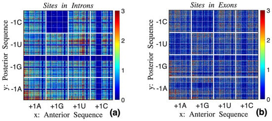
Figure 8. Point-sets for nucleic acid sites within (a) introns and (b) exons, both of which appear to be fractal. The two fractals appear to have distinct characteristics.

Visually, the two fractals appear to be different, with Figure 8b appearing more uniform than Figure 8a. It is extremely difficult to infer such features by direct analyses of nucleic acid sequences.

The objects shown in Figure 8 are multi-fractals, i.e., they are a collection of many fractal objects and can be characterized using multi-fractal spectra $f\left(\alpha \right)$ [64]. The computation requires partitioning the domain into (disjoint) squares and evaluating the set of probabilities $\left\{p_k\right\}$ of points within each square. The objects in Figure 8 are partitioned into squares of a fixed size, $\epsilon ={\left({\displaystyle \frac{1}{4}}\right)}^4$ and the probabilities $p_k$ were assessed in generating Figure 8. For each “moment” q, one computes the function $\tau \left(q\right)$ that satisfies

$$\sum _k{p}_k^q\sim {\epsilon }^{\tau \left(q\right)},$$

(5)

where the sum is taken over all members of the partition. The function $\tau \left(q\right)$ is monotonically increasing. The singularity spectrum is the Legendre transform of $\tau \left(q\right)$

$$\alpha ={\displaystyle \frac{d\tau \left(q\right)}{dq}};f\left(\alpha \right)=\alpha q-\tau \left(q\right).$$

(6)

Here, $\alpha$ distinguishes distinct fractals within the set, and $f\left(\alpha \right)$ is the fractal dimension of each set [64]. The fractal dimension of the full set is the maximum of the $f\left(\alpha \right)$ curve.

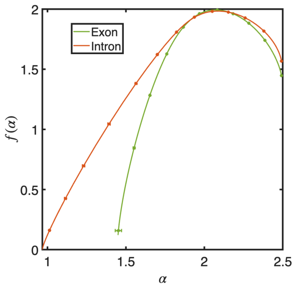
Points-sets within exons and introns were extracted from the UCSC Genome Browser [44], which contains approximately five million and a billion points, respectively. We used five randomly selected sub-groups of size 1,000,000 within each set for analysis, and we computed $\tau \left(q\right)$ for each group. The mean and standard errors for $\alpha$ and $f\left(\alpha \right)$ were evaluated for each q. The two $f\left(\alpha \right)$ curves shown in Figure 9 are different, especially for small values of $\alpha$. This difference quantifies the distinct features of high-density regions [64]. The overall fractal structures of nucleic acid sites within exons and introns are dissimilar.

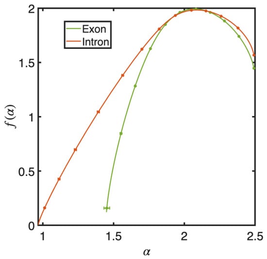
Figure 9. Singularity spectra for point-sets of nucleic acid sites in introns and exons. The error bars, except for the lowest $\alpha$ in the exon point-set, are too small to note. The spectra differ at small values of $\alpha$, signifying the enhanced presence of high-density regions within intron sequences, as can be observed from Figure 8.

3. Discussion

Although the splicing of pre-mRNA is a highly complex, multi-stage process involving a co-transcriptional synthesis of the dynamic ribonucleoprotein complex spliceosome [15,65,66,67,68,69,70], simpler facets—such as binding to the snRNAs $U1$, $U2$, and perhaps $U5$—may be amenable to in-depth analyses and yield important insights. The expectation is predicated on the recognition regions of snRNAs being small. However, even they can attach to multiple consensus sequences, as displayed via sequence logos [12,13,14].

Nucleic acid sequences in pre-mRNA are known to exhibit non-trivial statistical features, a well-known example being the low density of $CG$-dyads. A higher-order characteristic is the compensation effect, which asserts a strong correlation between the presence of guanine at $+5$ and $-1$ sites at exon–intron boundaries [38,39,40]. It is difficult to discover complex structural details through direct analyses of nucleic acid sequences. Point-sets were introduced as a visual display that can aid in such searches [41]. They are defined using sub-sequences on either side of a site of interest, under the assumption that, generally, nucleotides closer to the site will play a more significant role in its fate. In this paper, we focus on probability density functions in point-sets. These can be helpful in testing hypotheses on physical mechanisms that underlie (for example) the choice of consensus sequences. Addressing such queries requires not only comparisons of likelihoods of appearance, given by sequence logos, but of higher-order statistical measures as well.

Sequence neighborhoods of exon–intron boundaries extracted from databases were found to contain over a third of all possible sub-sequences. However, these sub-sequences are not random but highly structured. Their characteristics are succinctly displayed through point-sets. Point-sets and consensus sequences at branch points clearly depend on the nucleic acid at the branch point site (see Figure 4). Similar differences may be present in distinct classes of splicing, such as normal splicing and self-splicing [71,72,73], but it is difficult to find a sufficiently large dataset to implement a statistical analysis on the latter group. Although quantitative differences between branch point neighborhoods can be determined using the two-dimensional Kolmogorov–Smirnov test, the results provide little insight beyond what can be gleaned visually. Point-sets can also be helpful in highlighting differences between two classes of junctions, such as those between normal exon–exon junctions and cancer fusion junctions (see Figure 7). The ability to highlight such differences may aid in the search for the origins of diseases.

Machine learning algorithms such as SpliceAI [74,75,76] are highly effective at splice-site selection. However, they require several thousand nucleotides on either side of the site of interest for reliable identification, whereas such extensive information is unlikely to be accessible during splicing. One possibility is that machine learning algorithms can detect differences in the structural characteristics of nucleic acid sequences within exons and within introns. Our studies on the fractal nature of point-sets were motivated as a test of this possibility. Point-sets were indeed found to be fractal, and those associated with sites in introns and exons were dissimilar. The differences were quantified using singularity spectra [64].

We have presented several examples where probability density functions on point-sets permit us to gather information on the nature and characteristics of nucleic acid sub-sequences. These assertions and quantitative differentiations of nucleic acid sequences between different groups would be extremely difficult to infer without the use of point-sets.

References

- Goldberg, M.; Fischer, J.; Hood, L.; Hartwell, L.; Aquardro, C.; Silver, L.; Reynolds, A.E. Genetics: From Genes to Genomes, 7th ed.; McGraw-Hill Publishing: New York, NY, USA, 2021. [Google Scholar]
- Roca, X.; Krainer, A.R.; Eperon, I.C. Pick one, but be quick: 59 splice sites and the problems of too many choices. Genes Dev. 2013, 27, 129–144. [Google Scholar] [CrossRef]
- Sponer, J.; Leszczynski, J.; Hobza, P. Nature of nucleic acid-base stacking: Nonempirical ab initio and empirical potential characterization of 10 stacked base dimers. comparison of stacked and h-bonded base pairs. J. Chem. Phys. 1996, 100, 5590–5596. [Google Scholar] [CrossRef]
- Jurecka, P.; Sponer, J.; Cerny, J.; Hobza, P. Benchmark database of accurate (MP2 and CCSD(T) complete basis set limit) interaction energies of small model complexes, DNA base pairs, and amino acid pairs. Phys. Chem. Chem. Phys. 2006, 8, 1985–1993. [Google Scholar] [CrossRef]
- Olivia, R.; Cavallo, L.; Tramontano, A. Accurate energies of hydrogen bonded nucleic acid base pairs and triplets in tRNA tertiary interactions. Nucleic Acids Res. 2006, 34, 865–879. [Google Scholar] [CrossRef]
- Johnson, C.A.; Bloomingdale, R.J.; Ponnusamy, V.E.; Tillinghast, C.A.; Znosko, B.M.; Lewis, M. A computational model for predicting experimental RNA and DNA nearest-neighbor free energy rankings. J. Chem. Phys. 2011, 115, 9244–9251. [Google Scholar] [CrossRef]
- Jolley, E.A.; Lewis, M.; Znosko, B.M. A computational model for predicting experimental RNA nearest-neighbor free energy rankings: Inosine–Uridine pairs. Chem. Phys. Lett. 2015, 639, 157–160. [Google Scholar] [CrossRef] [PubMed]
- Leon, S.C.; Prentiss, M.; Fyta, M. Binding energies of nucleobase complexes: Relevance to homology recognition of DNA. Phys. Rev. E 2016, 93, 06210. [Google Scholar] [CrossRef]
- Hopfinger, M.C.; Kirkpatrick, C.C.; Znosko, B.M. Predictions and analyses of RNA nearest neighbor parameters for modified nucleotides. Nucleic Acids Res. 2020, 48, 8901–8913. [Google Scholar] [CrossRef] [PubMed]
- Parker, M.T.; Soanes, B.K.; Kusakina, J.; Larrieu, A.; Knop, K.; Joy, N.; Breidenbach, F.; Sherwood, A.V.; Barton, G.J.; Fica, S.M.; et al. m6A modification of U6 snRNA modulates usage of two major classes of pre-mRNA 5′ splice site. eLife 2022, 11, e78808. [Google Scholar] [CrossRef] [PubMed]
- Schneider, T.D.; Stephens, R.M. Sequence logos: A new way to display consensus sequences. Nucleic Acids Res. 1990, 18, 6097–6100. [Google Scholar] [CrossRef]
- Rogozin, I.B.; Milanesi, L. Analysis of donor splice sites in different eukaryotic organisms. J. Mol. Evol. 1997, 45, 50–59. [Google Scholar] [CrossRef]
- Sibley, C.R.; Blazquez, L.; Ule, J. Lessons from non-canonical splicing. Nat. Rev. Genet. 2016, 17, 407–421. [Google Scholar] [CrossRef] [PubMed]
- Hümmer, S.; Borao, S.; Guerra-Moreno, S.; Cozzuto, L.; Hidalgo, E.; Ayte, J. Cross talk between the upstream exon-intron junction and Prp2 facilitates splicing of non-consensus introns. Cell Rep. 2021, 37, 109893. [Google Scholar] [CrossRef]
- Wahl, M.C.; Will, C.L.; Lührmann, R. The spliceosome: Design principles of a dynamic RNP machine. Cell 2009, 136, 701–718. [Google Scholar] [CrossRef]
- Will, C.L.; Lührmann, R. Spliceosome structure and function. Cold Spring Harb. Perspect. Biol. 2011, 3, a003707. [Google Scholar] [CrossRef]
- Hertel, K.J. Spliceosomal Pre-mRNA Splicing Methods and Protocols, 1st ed.; Methods in Molecular Biology, 1126; Humana Press: Totowa, NJ, USA, 2014. [Google Scholar]
- Matera, A.G.; Wang, Z. A day in the life of the spliceosome. Nat. Rev. Mol. Cell Biol. 2014, 15, 108–121. [Google Scholar] [CrossRef] [PubMed]
- Merkhofer, E.C.; Hu, P.; Johnson, T.L. Introduction to co-transcriptional RNA splicing. In Spliceosomal Pre-mRNA Splicing: Methods and Protocols; Humana Press: Totowa, NJ, USA, 2014; pp. 83–96. [Google Scholar]
- Gilbert, W. Why genes in pieces? Nature 1978, 271, 501. [Google Scholar] [CrossRef]
- Kadri, N.K.; Mapel, X.M.; Pausch, H. The intronic branch point sequence is under strong evolutionary constraint in the bovine and human genome. Commun. Biol. 2021, 4, 1206. [Google Scholar] [CrossRef]
- Lasda, E.L.; Blumenthal, T. Trans-splicing. Wiley Interdiscip. Rev. RNA 2011, 2, 417–434. [Google Scholar] [CrossRef] [PubMed]
- Hiller, M.; Zhang, Z.; Backofen, R.; Stamm, S. Pre-mRNA secondary structures influence exon recognition. PLoS Genet. 2007, 3, e204. [Google Scholar] [CrossRef]
- Long, M.; Deutsch, M. Intron exon structures of eukaryotic model organisms. Nucleic Acids Res. 1999, 27, 3219–3228. [Google Scholar] [CrossRef]
- Zhu, L.; Zhang, Y.; Zhang, W.; Yang, S.; Chen, J.-Q.; Tian, D. Patterns of exon-intron architecture variation of genes in eukaryotic genomes. BMC Genom. 2009, 10, 47. [Google Scholar] [CrossRef]
- Wang, Y.; Liu, J.; Huang, B.O.; Xu, Y.-M.; Li, J.; Huang, L.-F.; Lin, J.; Zhang, J.; Min, Q.-H.; Yang, W.-M.; et al. Mechanism of alternative splicing and its regulation. Biomed. Rep. 2015, 3, 152–158. [Google Scholar] [CrossRef] [PubMed]
- Stepankiw, N.; Raghavan, M.; Fogarty, E.A.; Grimson, A.; Pleiss, J.A. Widespread alternative and aberrant splicing revealed by lariat sequencing. Nucleic Acids Res. 2015, 43, 8488–8501. [Google Scholar] [CrossRef] [PubMed]
- Ule, J.; Blencowe, B.J. Alternative splicing regulatory networks: Functions, mechanisms, and evolution. Mol. Cell 2019, 76, 329–345. [Google Scholar] [CrossRef] [PubMed]
- Marasco, L.E.; Kornblihtt, A.R. The physiology of alternative splicing. Nat. Rev. Mol. Cell Biol. 2023, 24, 242–254. [Google Scholar] [CrossRef]
- Walsh, C.E. New paradigm for gene transfer: RNA trans-splicing and small interfering RNA as therapeutic strategies. Semin. Hematol. 2004, 41, 297–302. [Google Scholar] [CrossRef]
- Yang, Y.; Walsh, C.E. Spliceosome-mediated RNA trans-splicing. Mol. Ther. 2005, 12, 1006–1012. [Google Scholar] [CrossRef]
- Cooper, T.A.; Wan, L.; Dreyfuss, G. RNA and disease. Cell 2009, 136, 777–793. [Google Scholar] [CrossRef]
- Mcmanus, C.J.; Duff, M.O.; Eipper-Mains, J.; Graveley, B.R. Global analysis of trans-splicing in Drosophila. Proc. Natl. Acad. Sci. USA 2010, 107, 12975–12979. [Google Scholar] [CrossRef]
- Scotti, M.M.; Swanson, M.S. RNA mis-splicing in disease. Nat. Rev. Genet. 2016, 17, 19–32. [Google Scholar] [CrossRef] [PubMed]
- Jiang, W.; Chen, L. Alternative splicing: Human disease and quantitative analysis from high-throughput sequencing. Comput. Struct. Biotechnol. J. 2021, 19, 183–195. [Google Scholar] [CrossRef]
- Aebersold, R.; Agar, J.N.; Amster, I.J.; Baker, M.S.; Bertozzi, C.R.; Boja, E.S.; Costello, C.E.; Cravatt, B.F.; Fenselau, C.; Garcia, B.A.; et al. How many human proteoforms are there? Nat. Chem. Biol. 2018, 14, 206–214. [Google Scholar] [CrossRef]
- van der Feltz, C.; Hoskins, A.A. Structural and functional modularity of the U2 snRNP in pre-mRNA splicing. Crit. Rev. Biochem. Mol. Biol. 2019, 54, 443–465. [Google Scholar] [CrossRef]
- Burge, C.; Karlin, S. Prediction of complete gene structures in human genomic DNA. J. Mol. Biol. 1997, 268, 78–94. [Google Scholar] [CrossRef]
- Carmel, I.; Tai, S.; Vig, I.; Ast, G. Comparative analysis detects dependencies among the 5′ splice-site positions. RNA 2004, 10, 828–840. [Google Scholar] [CrossRef]
- Artemyeva-Isman, O.V.; Porter, A.C.G. U5 snRNA interactions with exons ensure splicing precision. Front. Genet. 2021, 12, 676971. [Google Scholar] [CrossRef]
- Speakman, E.; Gunaratne, G.H. On a kneading theory for gene-splicing. CHAOS 2024, 34, 043125. [Google Scholar] [CrossRef]
- Iida, Y.; Sasaki, F. Recognition patterns for exon-intron junctions in higher organisms as revealed by a computer search. J. Biochem. 1983, 94, 1731–1738. [Google Scholar] [CrossRef] [PubMed]
- Kramárek, M.; Soucek, P.; Réblova, K.; Grodecká, L.K.; Freiberger, T. Splicing analysis of STAT3 tandem donor suggests non-canonical binding registers for U1 and U6 snRNAs. Nucleic Acids Res. 2024, 52, 5959–5974. [Google Scholar] [CrossRef] [PubMed]
- Perez, G.; Barber, G.P.; Benet-Pages, A.; Casper, J.; Clawson, H.; Diekhans, M.; Fischer, C.; Gonzalez, A.S.; Hinrichs, J.N.; Lee, C.M.; et al. The UCSC Genome Browser database: 2025 update. Nucleic Acids Res. 2025, 53, D1243–D1249. [Google Scholar] [CrossRef]
- Parker, M.T.; Fica, S.M.; Simpson, G.G. RNA splicing: A split consensus reveals two major 5’ splice site classes. Open Biol. 2025, 15, 240293. [Google Scholar] [CrossRef]
- Anna, A.; Monika, G. Splicing mutations in human genetic disorders: Examples, detection, and confirmation. J. Appl. Genet. 2018, 59, 253–268. [Google Scholar] [CrossRef]
- Mercer, T.R.; Clark, M.B.; Andersen, S.B.; Brunck, M.E.; Haerty, W.; Crawford, J.; Taft, R.J.; Nielsen, L.K.; Dinger, M.E.; Mattick, J.S. Genome-wide discovery of human splicing branchpoints. Genome Res. 2015, 25, 290–303. [Google Scholar] [CrossRef] [PubMed]
- Smirnov, N. Table for estimating the goodness of fit of empirical distributions. Ann. Math. Stat. 1948, 19, 279–281. [Google Scholar] [CrossRef]
- Peacock, J.A. Two-dimensional goodness-of-fit testing in astronomy. Mon. Not. R. Astron. Soc. 1983, 202, 615–627. [Google Scholar] [CrossRef]
- Fasano, G.; Franceschini, A. A multidimensional Kolmogorov-Smirnov test. Mon. Not. R. Astron. Soc. 1987, 225, 155–170. [Google Scholar] [CrossRef]
- Press, W.H.; Teukolsky, S.A. Kolmogorov-Smirnov test for two-dimensional data: How to tell whether a set of (x,y) data paints are consistent with a particular probability distribution, or with another data. Comput. Phys. 1988, 2, 74–77. [Google Scholar] [CrossRef]
- Faustino, N.A.; Cooper, T.A. Pre-mRNA splicing and human disease. Genes. Dev. 2003, 17, 419–437. [Google Scholar] [CrossRef] [PubMed]
- Graveley, B.R. The haplo-spliceo-transcriptome: Common variations in alternative splicing in the human population. Trends Genet. 2007, 24, 5–7. [Google Scholar] [CrossRef][Green Version]
- Fu, R.-H.; Liu, S.-P.; Huang, H.-J.; Chen, S.-J.; Chen, P.-R.; Lin, Y.-H.; Ho, Y.-C.; Chang, W.-L.; Tsai, C.-H.; Shyu, W.-C.; et al. Aberrant alternative splicing events in parkinson’s disease. Cell Transplant. 2013, 22, 653–661. [Google Scholar] [CrossRef]
- Chwalenia, K.; Facemire, L.; Li, H. Chimeric rnas in cancer and normal physiology. Wiley Interdiscip. Rev. RNA 2017, 8, e1427. [Google Scholar] [CrossRef] [PubMed]
- Montes, M.; Sanford, B.L.; Comiskey, D.F.; Chandler, D.S. Rna splicing and disease: Animal models to therapies. Trends Genet. 2018, 35, 68–87. [Google Scholar] [CrossRef]
- Zhang, Y.; Qian, J.; Gu, C.; Yang, Y. Alternative splicing and cancer: A systematic review. Signal Transduct. Target. Ther. 2021, 6, 78. [Google Scholar] [CrossRef] [PubMed]
- Sun, H.; Liu, K.; Yi, C. Regulation and functions of non-m6A mRNA modifications. Nat. Rev. Mol. Cell Biol. 2023, 24, 714–731. [Google Scholar] [CrossRef]
- Kim, P.; Yoon, S.; Kim, N.; Lee, S.; Ko, M.; Lee, H.; Kang, H.; Kim, J.; Lee, S. ChimerDB 2.0—A knowledge-base for fusion genes updated. Nucleic Acids Res. 2010, 38, D81–D85. [Google Scholar] [CrossRef] [PubMed]
- Kim, P.; Zhou, X. FusionGDB: Fusion gene annotation DataBase. Nucleic Acids Res. 2019, 47, D994–D1004. [Google Scholar] [CrossRef]
- Kim, P.; Tan, H.; Liu, J.; Lee, H.; Jung, H.; Kumar, H.; Zhou, H. FusionGDB 2.0: Fusion gene annotation updates aided by deep learning. Nucleic Acids Res. 2022, 50, D1221–D1230. [Google Scholar] [CrossRef]
- Woods, T.; Preeprem, T.; Lee, K.; Chang, W.; Vidakovic, B. Characterizing exons and introns by regularity of nucleotide strings. Biol. Direct 2016, 11, 6. [Google Scholar] [CrossRef][Green Version]
- Cain, J.A.; Montibus, B.; Oakey, R.J. Intragenic CpG islands and their impact on gene regulation. Front. Cell Dev. Biol. 2022, 10, 832348. [Google Scholar] [CrossRef]
- Halsey, T.C.; Jensen, M.H.; Kadanoff, L.P.; Procaccia, I.; Shraiman, B.I. Fractal measures and their singularities: The characterization of strange sets. Phys. Rev. A 1986, 33, 1141–1151. [Google Scholar] [CrossRef] [PubMed]
- Wan, R.; Bai, R.; Zhan, X.; Shi, Y. How is precursor messenger RNA spliced by the spliceosome? Annu. Rev. Biochem. 2020, 89, 333–358. [Google Scholar] [CrossRef]
- Gehring, N.H.; Roignant, J.-Y. Anything but ordinary—Emerging splicing mechanisms in eukaryotic gene regulation. Trends Genet. 2021, 37, 355–372. [Google Scholar] [CrossRef] [PubMed]
- Beusch, I.; Rao, B.; Studer, M.K.; Luhovska, T.; Sukyte, V.; Lei, S.; Oses-Prieto, J.; SeGraves, E.; Burlingame, A.; Jonas, S.; et al. Targeted high-throughput mutagenesis of the human spliceosome reveals its in vivo operating principles. Mol. Cell 2023, 83, 2578–2594. [Google Scholar] [CrossRef]
- Rogalska, M.E.; Vivor, C.; Valcárcel, J. Regulation of pre-mRNA splicing: Roles in physiology and disease, therapeutic prospects. Nat. Rev. Genet. 2023, 24, 251–269. [Google Scholar] [CrossRef]
- Shenasa, H.; Bentley, D.L. Pre-mRNA splicing and its co-transcriptional connections. Trends Genet. 2023, 39, 672–685. [Google Scholar] [CrossRef] [PubMed]
- Zhan, X.; Lu, Y.; Shi, Y. Molecular basis for the activation of human spliceosome. Nat. Commun. 2024, 15, 6348–6357. [Google Scholar] [CrossRef]
- Cech, T.R. The chemistry of self-splicing RNA and RNA enzymes. Science 1987, 236, 1532–1539. [Google Scholar] [CrossRef]
- Cech, T.R. Self-splicing and enzymatic activity of an intervening sequence RNA from Tetrahymena. Biosci. Rep. 1990, 10, 239–261. [Google Scholar] [CrossRef]
- Pyle, A.M. Group II intron self-splicing. Annu. Rev. Biophys. 2016, 45, 183–205. [Google Scholar] [CrossRef]
- Jaganathan, K.; Panagiotopoulou, S.K.; McRae, J.F.; Darbandi, S.F.; Knowles, D.; Li, Y.I.; Kosmicki, J.A.; Arbelaez, J.; Cui, W.; Schwartz, G.B.; et al. Predicting splicing from primary sequence with deep learning. Cell 2019, 176, 535–548. [Google Scholar] [CrossRef] [PubMed]
- de Sainte-Agathe, J.-M.; Filser, M.; Isidor, B.; Besnard, T.; Gueguen, P.; Perrin, A.; Van Goethem, C.; Verebi, C.; Masingue, M.; Rendu, J.; et al. Spliceai-visual: A free online tool to improve SpliceAI splicing variant interpretation. Hum. Genom. 2023, 17, 7. [Google Scholar] [CrossRef] [PubMed]
- Chao, K.-H.; Mao, A.; Liu, A.; Salzberg, S.L.; Pertea, M. OpenSpliceAI provides an efficient modular implementation of SpliceAI enabling easy retraining across nonhuman species. eLife 2025, 14, RP107454. [Google Scholar] [CrossRef] [PubMed]
Disclaimer/Publisher’s Note: The statements, opinions and data contained in all publications are solely those of the individual author(s) and contributor(s) and not of MDPI and/or the editor(s). MDPI and/or the editor(s) disclaim responsibility for any injury to people or property resulting from any ideas, methods, instructions or products referred to in the content. |
© 2026 by the authors. Licensee MDPI, Basel, Switzerland. This article is an open access article distributed under the terms and conditions of the Creative Commons Attribution (CC BY) license.