An Algorithm for Numerical Integration of ODE with Sampled Unknown Functional Factors

Abstract

The problem of having ordinary differential equations (ODE) whose coefficients are unknown functions is frequent in several fields. Sometimes, it is possible to obtain samples of the values of these functions in different instants or spatial points. The present paper presents a methodology for the numeric solving of these ODE. There are approximations to the problem for specific cases of equations, especially in the case where the parameters correspond to constants. Other studies focus on the case in which the functions under consideration are linear or meet a certain condition. There are two main advantages of the proposed algorithm. First, it does not impose any condition over the data or the subsequent function from where these sample data are derived. Additionally, the methodology used in the functions modeling can control the possibility of overfitting in the function modeling. This is a crucial point in order to limit the influence of model biases in the numerical solution of the ordinary differential equation under study.

1. Introduction

In the study and modeling of systems, differential equations can be obtained with parameters that depend on observations. That is, they are parameters that can vary throughout the domain of definition and for which experimental data are known. Differential equations can be either ordinary differential equations or partial differential equations. Problems modeled by this type of differential equations are, for example, (see [1,2,3,4,5]): (a) the heat equation with unknown specific heat and heat sources; (b) the diffusion equation of products with non-constant and unknown innovation and imitation coefficients; (c) the study of hydraulic transients; and (d) water flows such as groundwater seepage in anisotropic media. In this sense, it is important to obtain hybrid-modeling methodologies that allow combining parameter estimation methods with algorithms of numerical resolution of differential equations.

When the dynamics of the processes underlying the system under study are known, differential equations can model their behavior, especially in the case of complex dynamic processes. In many cases, these differential equations contain constant parameters or functional dependencies with the independent variable that determine the characteristics of the corresponding solutions. The exact knowledge of its parameters is crucial for predicting the behavior of the solutions. Some concrete examples of the study of the problem considered in specific fields could be, for example, in biology and ecology [6,7,8], chemistry [9,10], electronics [11] and engineering [12,13].

The problem of determining the constant coefficients present in a differential equation from the study of the solutions of the system has been the subject of different studies, presenting a variety of methods of resolution. First approaches were based on least squares techniques. However, due to the absence of an analytical solution, the need to solve the ODEs numerically makes this approach computationally expensive. An alternative is the generalized profiling estimation method, where the solution is approximated using a linear combination of basis functions and adjusting the coefficients of the corresponding expansion equation by comparing them with the differential equation (see [14,15]). This method is applied even in the case in which the model is stochastic [16]. A study on the properties of this type of algorithm can be found in [17]. Other investigations are based on the use of non-deterministic methods (for example genetic algorithms [18], particle swarm optimization [10]) or Machine Learning (ML) techniques. Some studies focus on methods applicable to specific types of equations. For example [19], where the problem corresponds to a differential equation associated with the time evolution of a system, and is solved by making a large number of observations of the evolution of the system over short intervals.

However, the application of the techniques discussed in real problems presents a series of difficulties due to the characteristics of the numerical data available in such cases, as discussed in [20]. In addition, the presence of outliers makes it necessary to design and use robust algorithms, see, for example, [21]. There are also some considerations that complicate the efficient use of some of the methods. For example, in stiff problems, the presence of nonlinearity in the solution space [10] or high dimensionality of the parameters space, in partial differential equations (PDE) [12].

The approach taken in the present investigation is in a certain way the inverse of that of the cases previously considered. It is proposed to obtain a solution of the differential equations by previously determining the values of the parameters that best fit the observations made. However, the approach used in [10] has a certain similarity in its first stages to the one presented in this paper.

When the function to model corresponds to a spatial-distributed variable, kriging is usually used as the best linear estimator of the function from a set of random measurements. This can be found in the work of [22,23] for the calculation of unknown coefficients in linear PDE [24,25].

The proposal presented in this research work performs a modeling of the parameters of the differential equation in the case of functional dependence, by means of a local regression method based on the finite element method. Therefore, a brief introduction to the modeling methods will be given below.

The number of techniques available to model a relationship between variables is large. Selecting one or another depends on a variety of factors, from the data itself to the knowledge of the underlying equation involving the variables. The toolbox goes from classical statistical methods as linear or multilinear regression to machine-learning oriented methods as neural networks and related techniques, random trees, support vector regression and others.

The problem under consideration consists of obtaining a model of the relationship between a set of variables that is assumed to be determined by a function $f:\Omega \subset {ℝ}^d\to ℝ$

$$y=f\left(x^1,\dots ,x^d\right).$$

(1)

All the considered methods start from an experimental dataset $\mathsf{{\rm Y}}$ of P tuples sampled from the relation (1):

$$\mathsf{{\rm Y}}={\left\{\left(x_{\left[k\right]}^1,x_{\left[k\right]}^2,x_{\left[k\right]}^3,\dots ..,x_{\left[k\right]}^d,y_{\left[k\right]}\right)\right\}}_{k=1,2,\dots .,P},$$

(2)

where, for every $k=1,2,\dots .,P$ is verified $\left(x_{\left[k\right]}^1,x_{\left[k\right]}^2,x_{\left[k\right]}^3,\dots ..,x_{\left[k\right]}^d,y_{\left[k\right]}\right)\in \Omega \times ℝ$.

The literature developing the different methods can be easily accessed and they are widely applied to a variety of problems. From these data, each methodology allows us to obtain estimates of the values of $f\left(x^1,\dots ,x^d\right)$ at each point of $\Omega$ using an algorithm:

$$\begin{array}{c}F:\Omega \subset {ℝ}^d\times {ℝ}^J\to ℝ\\ \left(x^1,\dots ,x^d;{\theta }^1,\dots ,{\theta }^J\right)⟼F\left(x^1,\dots ,x^d;{\theta }^1,\dots ,{\theta }^J\right)\end{array},$$

(3)

where $\left({\theta }^1,\dots ,{\theta }^J\right)$ represents a set of parameters specific to each methodology and which determines the output value of the model. These estimated values will be denoted by:

$$\widehat{y}=F\left(x^1,\dots ,x^d;{\theta }^1,\dots ,{\theta }^J\right).$$

(4)

The methods for numeric model estimation are usually stated as a minimization problem over some kind of global error $E$ obtained as a function $H:{ℝ}^P\to ℝ$ of individual errors ${\epsilon }_{\left[k\right]}$ defined over the sampled and estimated values:

$$E=H\left({\epsilon }_{\left[1\right]},{\epsilon }_{\left[2\right]},\dots .,{\epsilon }_{\left[P\right]}\right)$$

(5)

with ${\epsilon }_{\left[k\right]}=y_{\left[k\right]}-{\widehat{y}}_{\left[k\right]}=y_{\left[k\right]}-F\left(x_{\left[k\right]}^1,\dots ..,x_{\left[k\right]}^d;{\theta }^1,\dots ,{\theta }^J\right)$.

Thus considered, the function H allows the approach of an optimization problem (see Equation (6)). Then, the optimal values $\left({\theta }_{*}^1,\dots ,{\theta }_{*}^J\right)$ that minimize the value of H for the available dataset are sought.

$$H\left(y_{\left[1\right]}-F\left(x_{\left[1\right]}^1,\dots ,x_{\left[1\right]}^d;{\theta }^1,\dots ,{\theta }^J\right),\dots ,y_{\left[P\right]}-F\left(x_{\left[P\right]}^1,\dots ,x_{\left[P\right]}^d;{\theta }^1,\dots ,{\theta }^J\right)\right).$$

(6)

These optimum parameters define the final model $F_{*}$ as:

$$F_{*}\left(x^1,\dots ,x^d;{\theta }_{*}^1,\dots ,{\theta }_{*}^J\right).$$

(7)

The present work follows the previous line of research developed by the authors with methodologies based on the finite elements method (FEM), a method for finding numerical solutions to differential equations with boundary conditions, developed initially to be applied in civil and aeronautical engineering [26,27,28,29,30,31].

In the following, in order to simplify notation, the criterion of writing the d-dimension points as a single variable will be used. Let us consider a given differential equation defined by a differential operator $D$, acting on a domain $\Omega \subset {ℝ}^d$:

$$D\left(f\right)=v,$$

(8)

where $f,v \in V\left(\Omega \right)$, $V$ being a function space defined over $\Omega$.

The finite element method replaces the domain $\Omega$ of $V$ by a collection of $N_e$ closed sets $\left\{{\Omega }_1,\dots ,{\Omega }_{N_e}\right\}$ called elements, that verify:

$$\begin{array}{c}{{\displaystyle \mathrm{U}}}_{j=1}^{N_e}{\Omega }_j=\Omega \\ {\Omega }_{j_1}\cap {\Omega }_{j_2}=\partial {\Gamma }_{j_1}\cap \partial {\Gamma }_{j_2}\end{array},$$

(9)

where $\partial {\Gamma }_j$ is the frontier of the closed ${\Omega }_j$.

This process is called meshing and it is usually done using sets of specific geometries, for example, in two dimensional triangles or rectangles. The generated mesh has an associated number that is related to the size of the elements. This parameter is usually denoted by $h$ and relates to the order of the error in the interpolations that will be defined in the next paragraph:

$$h=\underset{\rho ϵℝ}{\min }\left\{B\left(x_j,\rho \right)\supset {\Omega }_j \left| x_j\in {\Omega }_j\right., j=1, \dots ,N_e\right\},$$

(10)

where $B\left(x_j,\rho \right)$ is the open ball centred in $x_j$ with radius $\rho$.

Meshing on a domain also defines a set of Q points called nodes $\left({\zeta }_1, {\zeta }_2,\dots \dots ,{\zeta }_Q\right)$ that are used as support for the interpolation of any function defined on $\Omega$ through a related set of functions called shape functions $\left({\phi }_1\left(x\right),{\phi }_2\left(x\right),\dots \dots ,{\phi }_Q\left(x\right)\right)$ verifying the following conditions at the nodes:

$${\phi }_i\left({\zeta }_j\right)={\delta }_{ij},$$

(11)

for every $i,j=1,\dots ,Q$.

The linear span defined from the set of functions $\left({\phi }_1\left(x\right),{\phi }_2\left(x\right),\dots \dots ,{\phi }_Q\left(x\right)\right)$ forms a finite dimensional subspace which is composed by continuous piecewise polynomial functions of degree K (Sobolev space). This vector space is associated with a given division of the domain where the problem is set in and it will be denoted by $V_h$. That is:

$$V_h=span\left({\phi }_1\left(x\right),{\phi }_2\left(x\right),\dots \dots ,{\phi }_Q\left(x\right)\right).$$

(12)

On the space $V_h$, a derivative operator $D_h$ that generalizes the usual derivative to the functions of $V_h$ that are not derivable at all points of $\Omega$ can be defined.

The original problem can now be posed by searching the function $f_h ϵ V_h$:

$$f_h\left(x\right)={\sum }_{i=1}^Q{u}_i·{\phi }_i\left(x\right)$$

(13)

that best approximates the equation:

$$D_h\left(f_h\right)=v_h,$$

(14)

where $v_h ϵ V_h$ is the function of $V_h$ that corresponds with the interpolation of $v\left(x\right)$ defined in Equation (8).

The application of the FEM to the modelling of systems developed by the authors is based on the principle of projection through interpolation of any function $f \in V\left(\Omega \right)$ in the space $V_h$ as:

$$f\left(x\right)={\sum }_{i=1}^Q{\alpha }_i·{\phi }_i\left(x\right)\begin{array}{c}F:\Omega \subset {ℝ}^d\times {ℝ}^J\to ℝ\\ \left(x^1,\dots ,x^d;{\theta }^1,\dots ,{\theta }^J\right)⟼F\left(x^1,\dots ,x^d;{\theta }^1,\dots ,{\theta }^J\right)\end{array},$$

(15)

where ${\alpha }_i=f\left({\zeta }_i\right)$.

The numerical regression model for the relation Equation (1) will consist of the determination of the values $\left\{{\alpha }_1,\dots ,{\alpha }_Q\right\}$ that minimize an error function defined in a similar way to that in Equation (5).

The authors have been developing regression techniques based on Equation (15) as a method of approximation [32,33,34,35]. The last proposal is given by the octahedric regression methodology that will be presented in the next section.

The rest of the paper is organized as follows: Section 2 presents the basics of the modelling technique used in the proposed methodology, the octahedric regression and a study on the overfitting control and the computational algorithm. Section 3 presents four application examples. The first three correspond to the static heat equation and the last one to the Bass equation. Finally, Section 4 presents an analysis of the results obtained and a description of the computational characteristics of the methodology, together with a reflection on future lines of research.

2. Materials and Methods

The problem under consideration can be divided into two different phases: first, a model for the coefficients of the equation is determined. After this model has been obtained, it can be used to solve the differential equation using a typical numerical method, as those based on Runge–Kutta or multistep approaches.

In this section, we will proceed to the explanation of the modeling method to be used to estimate the coefficient functions at the nodes where the approximate numerical function is calculated. The following section presents the proposed solution to deal with the problem of overfitting, which is common to the techniques of modeling from experimental data. The last subsection develops the algorithm in the form of pseudocode, commenting on its main features.

2.1. Octahedric Regression

The problem of obtaining a model for the functional coefficients will be solved using the technique developed by the authors, called octahedric regression, and is presented in the research paper [36]. This algorithm presents good properties with respect to the following points: easy detection and control of the overfitting problem, efficient parallelization based on its embarrassing parallelism and fast numerical estimation for out of sample points.

Octahedral regression is an evolution of the previous numerical methodologies developed by the authors and corresponds to the fastest and most efficient of them. The next paragraphs provide a brief presentation of the basis of this methodology.

The basis is the use of parameterized radial functions, defined in the following point.

Definition 1. 

A radial function is a function$\Phi :{ℝ}_{+}x{ℝ}_{+}\to {ℝ}_{+}$that accomplishes the conditions

$$\left.\begin{array}{c}\forall \omega \ne 0 \underset{r\to \infty }{\lim }\Phi \left(r,\omega \right)=0\\ \forall r\ne 0 \underset{\omega \to 0}{\lim }\Phi \left(r,\omega \right)=0\end{array}\right\}.$$

(16)

The next definition introduces the averaged value estimator for a function at any point. In the following points, it is assumed that a radial function $\Phi \left(r,\omega \right)$ is selected and that the conditions on the functions for the existence of the corresponding integrals are satisfied.

Definition 2. 

Given a function$f:\Omega \subset {ℝ}^d\to ℝ$, the weighted average regression$c^{*}\left(x_o\right)$of$f$at$x_o\in \Omega$is defined using the implicit definition:

$$c^{*}\left(x_o\right)·W^0\left(x_o\right)-{\int }_{\Omega }^{}f\left(x\right)·\Phi \left(\Vert x-x_o\Vert ,\omega \right) dx=0\left.\begin{array}{c}\forall \omega \ne 0 \underset{r\to \infty }{\lim }\Phi \left(r,\omega \right)=0\\ \forall r\ne 0 \underset{\omega \to 0}{\lim }\Phi \left(r,\omega \right)=0\end{array}\right\},$$

(17)

where$W^0\left(x_o\right)={\int }_{\Omega }^{}\Phi \left(\Vert x-x_o\Vert ,\omega \right) dx$and$\Phi \left(\Vert x-x_o\Vert ,\omega \right)$are a function as presented in Definition 1.

In order to reduce the bias that may exist when calculating the previous weighted average, a set of points is introduced that will be used in the final estimation of the model.

Definition 3. 

Given a point$x_oϵ \Omega$and a parameter$h$(in the model is called pseudocomplexity), the octahedric support of size$h$around$x_o$is the set of$2·d$points:

$$\left\{x_o+\frac{h}{2}·e_1,x_o+\frac{h}{2}·e_2,\dots ..,x_o+\frac{h}{2}·e_d,x_o-\frac{h}{2}·e_1,x_o-\frac{h}{2}·e_2,\dots ..,x_o-\frac{h}{2}·e_d\right\},$$

(18)

where${\left\{e_j\right\}}_{j=1}^d$are the vectors of the canonical basis of${ℝ}^d$.

Definition 4. 

The octahedric regression model of$f\left(x\right)$at$x_o$is defined as the average of the weighted average regressions$c^{*}\left(x_o\pm \frac{h}{2}\cdot e_j\right)$calculated at the points of the octahedric support introduced in Definition 3. This estimated value will be denoted by$\widehat{f}\left(x_o\right)$and is given by:

$$\widehat{f}\left(x_o\right)=\frac{1}{2d}·{\sum }_{j=1}^d \left[c^{*}\left(x_o+\frac{h}{2}·e_j\right)+c^{*}\left(x_o-\frac{h}{2}·e_j\right)\right].$$

(19)

The following proposition shows the nature of the proposed estimator.

Proposition 1. 

The octahedric estimation$\widehat{f}\left(x_o\right)$of$f\left(x\right)$at$x_o$is a correction of order two with respect to the weighted average regression$c^{*}\left(x_o\right)$at the same point.

Demonstration. Developing the $c^{*}\left(x_o\pm \frac{h}{2}·e_j\right)$ functions in Equation (19) and $\Phi \left(\Vert x-x_o\pm \frac{h}{2}·e_j\Vert ,\omega \right)$ through the implicit definition given in Equation (17) in powers of h, the first order term cancels and the following expression holds:

$$\widehat{f}\left(x_o\right)=c^{*}\left(x_o\right)+O\left(h^2\right).$$

(20)

Equation (20) shows that octahedric regression is a correction of order $h^2$ to the weigthed average for central objective points. Consequently, when $h\to 0$, both values tend to coincide $\widehat{f}\left(x_o\right)\to c^{*}\left(x_o\right)$, causing overfitting on the points of the sample with respect to the points nearest to $x_o$. The way to study the existence and importance of this effect is through a second estimation called restricted model, where in the calculation of the model at a point, the corresponding values are removed from the sample in the case of being part of it. The results will be discussed in the next subsection.

When the problem is modelling a function from a discrete sample of size P (see Equation (2)) of points and values of $f\left(x\right)$, the integrals must be calculated using finite sums, so:

$$W^0\left(x_o\right)={\int }_{\Omega }^{} \Phi \left(\Vert x-x_o\Vert ,\omega \right) dx\cong \frac{1}{P}·{\sum }_{k=1}^P\Phi \left(\Vert x_k-x_o\Vert ,\omega \right)$$

(21)

$${\int }_{\Omega } f\left(x\right)·\Phi \left(\Vert x-x_o\Vert ,\omega \right) dx\cong \frac{1}{P}·{\sum }_{k=1}^P{y}_k·\Phi \left(\Vert x_k-x_o\Vert ,\omega \right).$$

(22)

Then, the discrete version of Equation (17) is:

$${\sum }_{k=1}^P\left[c^{*}\left(x_o\right)-x_k\right]·\Phi \left(\Vert x_k-x_o\Vert ,\omega \right)=0.$$

(23)

2.2. Control of Model Overfitting

From the result of Proposition 1, the trend to overfitting has been discussed. In this point, the question will be considered further.

Let us study the problem of estimating the value of an objective function $f\left(x\right)$ at the first point of the sample $x_1\in {\rm Y}$, and suppose that the rest of the points on the sample are ordered depending on the distance to $x_1$. Taking Equation (21) at the support points $x_1\pm \frac{h}{2}·e_j$,

$$W^0\left(x_1\pm \frac{h}{2}·e_j\right)\approx \Phi \left(\frac{h}{2},\omega \right)·\left\{1+\frac{\Phi \left(\Vert x_2-x_1\mp \frac{h}{2}·e_j\Vert ,\omega \right)}{\Phi \left(\frac{h}{2},\omega \right)}+..+\frac{\Phi \left(\Vert x_P-x_1\mp \frac{h}{2}·e_j\Vert ,\omega \right)}{\Phi \left(\frac{h}{2},\omega \right)}\right\}$$

(24)

The term on brackets represents the relative weight of each sample point in the weighted average. Summing up the contributions on each support point, the result can be written as:

$$1+\Psi \left(x_2-x_1,\omega \right)+..+\Psi \left(x_P-x_1,\omega \right),$$

(25)

where

$$\Psi \left(x_k-x_l,\omega \right)=\frac{{\sum }_{j=1}^d\left\{\Phi \left(\Vert x_k-x_l-\frac{h}{2}·e_j\Vert ,\omega \right)+\Phi \left(\Vert x_k-x_l+\frac{h}{2}·e_j\Vert ,\omega \right)\right\}}{2·\mathrm{d}·\Phi \left(\frac{h}{2},\omega \right)}.$$

(26)

The value of

$$\Pi \left(x_r\right)=1+{\displaystyle \sum }_{k\ne r}^P\Psi \left(x_k-x_r,\omega \right)$$

(27)

represents the weight of all the points in the estimation of the model calculated at $x_r$. At zero order in h, Equation (27) is approximately:

$$\Pi \left(x_r\right)\cong 1+\frac{{\sum }_{k\ne r}^P\Phi \left(\Vert x_k-x_r\Vert ,\omega \right)}{\Phi \left(\frac{h}{2},\omega \right)}.$$

(28)

By Equation (16), the fractions converge very fast to zero as the distance to $x_r$ grows, and the only contribution depends on the points that are at a distance similar to the nearest point, that is, when $\Phi \left(\Vert x_k-x_r\Vert ,\omega \right)\approx \Phi \left(\frac{h}{2},\omega \right)$. The number $q\left(\omega \right)$ of points involved is determined by the value of the parameter $\omega$, and $c^{*}\left(x_r\right)$ is a weighted mean of the q-nearest points. Therefore, the octahedric regression presented in the present paper corresponds to a mean of a simpler estimator calculated on the support of size h defined around $x_r$. These simple estimators correspond to the weighted average of the $q\left(x_r,\omega \right)$-nearest neighbors. In the limit $\omega \to 0$, $c^{*}\left(x_r\pm h·e_j\right)$ are obtained from the nearest point. In the case of considering all the experimental points, the model is called full. In that case, when $h\ll 1$, the nearest to the support points will very frequently be $x_r$, and then: $c^{*}\left(x_r\pm h·e_j\right)\to y_r$, and according to Equation (20), $\widehat{f}\left(x_r\right)\to y_r$, confirming the trend to overfitting.

The overfitting is caused by the incorporation of noise to the model. If the point that is being calculated is not included in the estimation, the points that are used to obtain the values of $c_i^{*}\left(x_r\pm h·e_j\right)$ have a greater probability of presenting independent noise influence, diminishing the overfitting in that form. The new model calculated in this form is called restricted and corresponds to having a cross-validation for each experimental point where the test set is formed by itself.

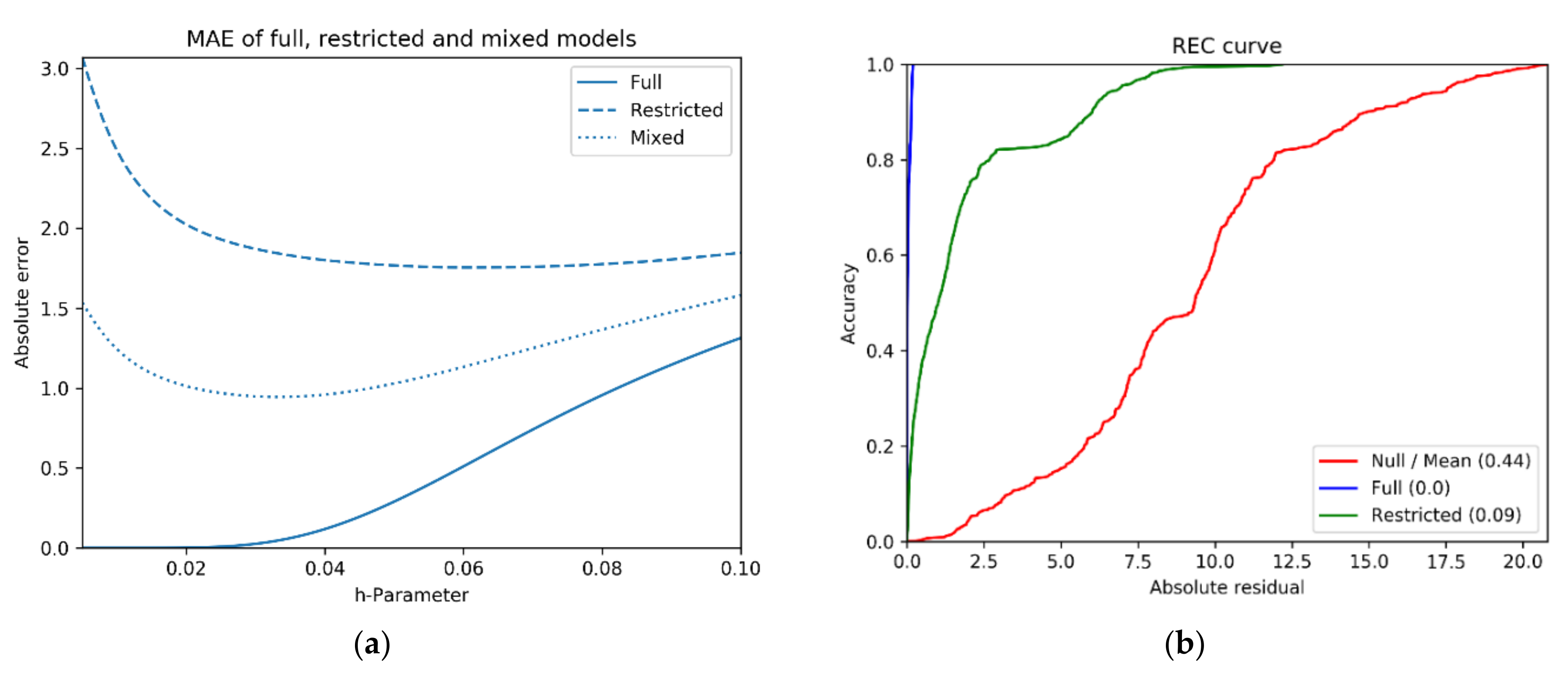
It has been commented previously that the methodology trends to overfitting when the size of the parameter h is small. Now, a real case of the application of octahedric regression will be shown in order to illustrate how this problem can be treated. Different statistical coefficients can be used to quantify the goodness of fit of a model. For example, the mean absolute error or REC curves. The example is a resume of the results presented in [36]. The first step is to calculate the so-called full and restricted models for different values of the parameter h.

As Figure 1a shows, the mixed model, calculated as the average of the errors of the restricted and full models, presents a minimum that can be used to fix the best value of the parameter h in the estimation process.

2.3. Computational Algorithm

The second step of the global algorithm corresponds with the numeric integration of the ordinary differential equation. As is well known, there is a variety of general algorithms and methods and, depending on the concrete ODE under study, some specific methodologies can be considered.

In the present research, the numerical method of integration used in the calculations corresponds to the predictor-corrector method based on the fourth-order multi-step Adams–Bashforth and Adams–Moulton algorithms. In these methods, it is necessary to calculate the unknown functional parameters at the nodes, so the regression model is used to estimate these values.

The exact form for the algorithm depends on the ODE under study. Algorithm 1 corresponds to the differential equation solved presented in Section 3.1:

$$\frac{d}{dx}\left(\alpha \left(x\right)·\frac{du}{dx}\right)=f\left(x\right).$$

(29)

Following Equations (21)–(23), the algorithm can be condensed in the next schema (Algorithm 1), where Euler’s method has been used in the numerical solution of the equation:

Algorithm 1. Sampled factors ODE numerical integrator

Input:

$N$: Number of intervals,  $a$: Left interval extreme,  $b$: Right interval extreme,  $w$: Parameter of radial function,  $x_1^{\left(s\right)},..,x_P^{\left(s\right)}$: Sample of independent variable,  ${\alpha }_1^{\left(s\right)},..,{\alpha }_P^{\left(s\right)}$: Sample of alpha function,  $f_1^{\left(s\right)},..,f_P^{\left(s\right)}$: Sample of f function,

Output:

$x_0,..,x_N$: Coordinates of nodes,  $u_0^{\left(0\right)},..,u_N^{\left(0\right)}$: Estimated numerical function,  $u_0^{\left(1\right)},..,u_N^{\left(1\right)}$: Estimated numerical derivative

Procedure IntegratingODE

$h\leftarrow \left(b-a\right)/N$

/* Modeling unknown functions at nodes*/

for $\mathrm{i}\leftarrow 0, N$ do

$x_i\leftarrow x_i+i·h$

$W^0\leftarrow 0$    See Equation (21)

$S_{\alpha }\leftarrow 0$    See Equation (22)

$S_f\leftarrow 0$    See Equation (22)

for $\mathrm{k}\leftarrow 0, P$ do

$\rho \leftarrow \Phi \left(x_i,x_k^{\left(s\right)},w\right)$

$W^0\leftarrow W^0+\rho$

$S_{\alpha }\leftarrow S_{\alpha }+\rho ·{\alpha }_k^{\left(s\right)}$

$S_f\leftarrow S_f+\rho ·f_k^{\left(s\right)}$

$\widehat{{\alpha }_i}\leftarrow S_{\alpha }/W^0$    See Equation (23)

$\widehat{f_i}\leftarrow S_f/W^0$    See Equation (23)

/* Initial conditions */

$u_0^{\left(1\right)}\leftarrow y_0^{\prime }·\widehat{{\alpha }_0}$

$u_0^{\left(0\right)}\leftarrow y_0$

/* Calculating numerical solution (Euler’s method)*/

for $\mathrm{i}\leftarrow 0, N-1$ do

$u_{i+1}^{\left(1\right)}\leftarrow u_i^{\left(1\right)}+\widehat{f_i}·h$

$u_{i+1}^{\left(0\right)}\leftarrow u_i^{\left(0\right)}+u_i^{\left(1\right)}·h/\widehat{{\alpha }_i}$

return $\left\{x_0,\dots ,x_N\right\},\left\{u_0^{\left(0\right)},\dots ,u_N^{\left(0\right)}\right\},\left\{u_0^{\left(1\right)},\dots ,u_N^{\left(1\right)}\right\}$

3. Results

To test the behavior of the proposed methodology, several examples are solved. First, two cases of the one-dimensional static inhomogeneous heat equation will be studied. Later, the Bass equation is analyzed to consider a different example.

Let us denote the solution to the differential equations on an interval $I=\left[a,b\right]$ by u(x).

For a given selection of standard deviation ($\sigma$) and sample size (P), the functional parameters are sampled and generate the corresponding numerical solutions for the equations. Denoting the set of samples by $S\left(P,\sigma \right)$ and each individual sample by $s\in S\left(P,\sigma \right)$, the solution can be represented as $u_s\left(x\right)$. In the examples, 200 iterations with different samples of the characteristic functions of the equation are run. From this set of solutions, the following statistical indexes are considered:

$$\overline{U}\left(x,P,\sigma \right)=\underset{s\in S\left(P,\sigma \right)}{\max }{u}_s\left(x\right)$$

(30)

$$\underset{\_}{U}\left(x,P,\sigma \right)=\underset{s\in S\left(P,\sigma \right)}{\min }{u}_s\left(x\right)$$

(31)

$$\langle U\left(P,\sigma \right)\rangle =u\left(b\right)-\langle u_s{\left(b\right)\rangle }_{s\in S\left(P,\sigma \right)}$$

(32)

$$U_M\left(P,\sigma \right)=u\left(b\right)-\underset{s\in S\left(P,\sigma \right)}{\mathrm{median}}{u}_s\left(b\right).$$

(33)

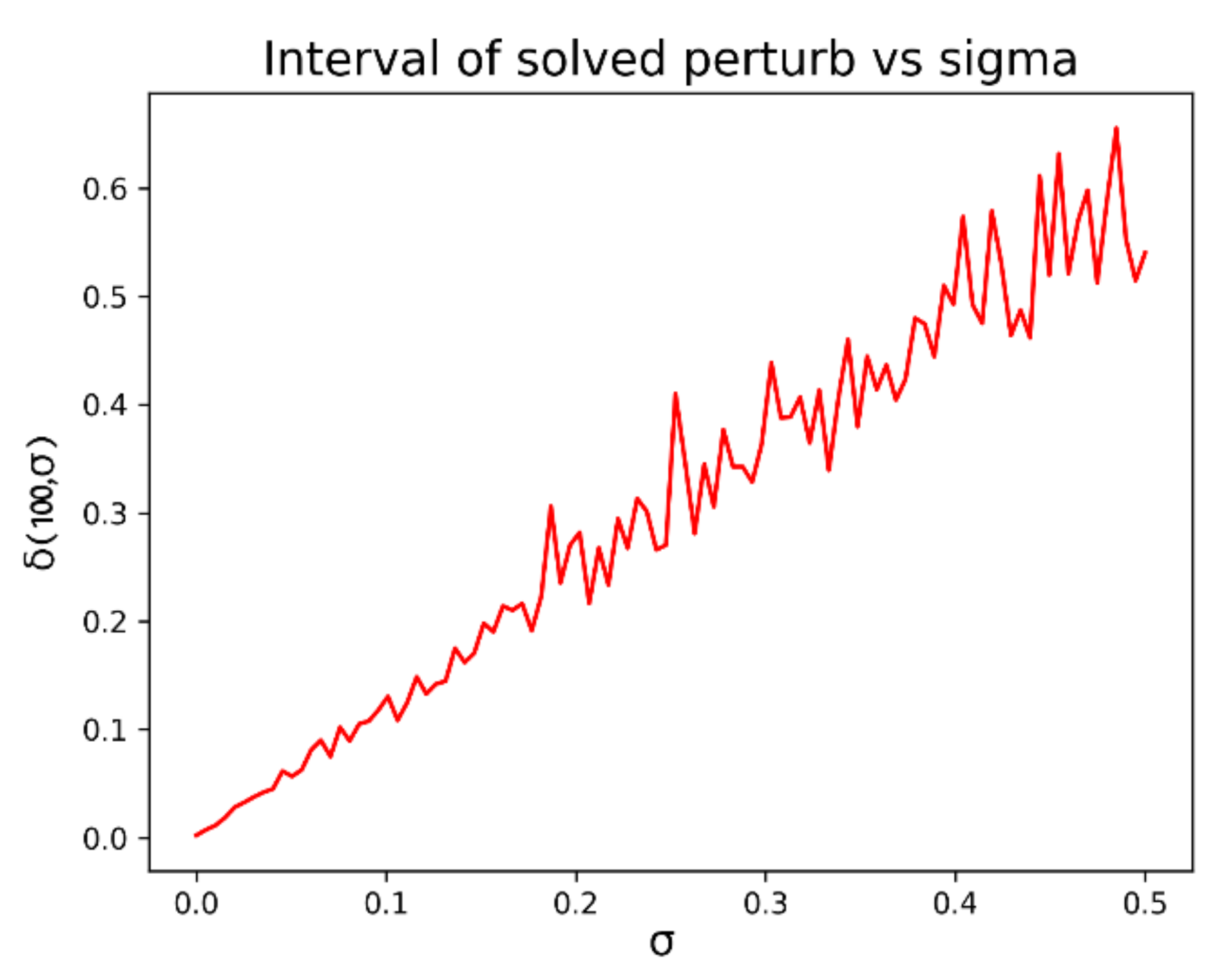
$\overline{U}\left(x,P,\sigma \right)$ and $\underset{\_}{U}\left(x,P,\sigma \right)$ represent the extreme values of the solutions at each point $x$ for a given sample size n and standard deviation $\sigma$. The amplitude of the difference $\delta \left(P,\sigma \right)=\underset{x\in \left[a,b\right]}{\max }\left\{\overline{U}\left(x,P,\sigma \right)-\underset{\_}{U}\left(x,P,\sigma \right)\right\},$ shows the size of variations in the solutions related to a given value of P and $\sigma$.

These indexes can be greatly influenced by low frequent extreme values, so additional parameters must be considered. For example, in the case that the exact solution is known, something frequent when studying the behavior of the algorithm, the average (Equation (32)) and median (Equation (33)) of the error calculated over the samples $s\in S\left(P,\sigma \right)$ can be a more convenient approach when studying the behavior of the solutions and their dependence on the magnitude of the perturbation.

The testing process followed these steps:

• Selection of the different standard deviation values ${\left\{{\sigma }_{\left[j\right]}\right\}}_{j=1}^{N_{\sigma }}$ for the perturbation (see next point) with which the study is to be carried out. The following steps should be performed once for each value of $\sigma \in {\left\{{\sigma }_{\left[j\right]}\right\}}_{j=1}^{N_{\sigma }}$ in the above set and as many times as indicated by the number of iterations (see Table 1, Table 2, Table 3 and Table 4);
• Generation of function samples from the uniform distribution $X\sim \mathcal{U}\left(a,b\right)$ for the points coordinates and a random normal distribution for the perturbation $ϵ\sim N\left(0,\sigma \right)$ as follows:

  $$Y^{\left(i\right)}=f^{\left(i\right)}\left(X\right)+ϵ,$$

  (34)

  where $f^{\left(i\right)}\left(x\right)$ represents the i-th functional parameter of the ODE under study and $Y^{\left(i\right)}$ is the corresponding sample. The size of each sample is specified in Table 1, Table 2, Table 3 and Table 4;
• Once the number of intervals $N$ has been selected, the model is obtained at the $N$+1 nodes obtained by dividing the interval $I=\left[a,b\right]$ into $N$ sub-intervals;
• Numerical resolution of the equation using the values of the functional parameters at the nodes obtained in the previous step, by means of an ordinary ODE resolution method, in the present case predictor-corrector;
• Calculation of statistical values $\overline{U}\left(x,P,\sigma \right)$, $\underset{\_}{U}\left(x,P,\sigma \right)$, $U\left(P,\sigma \right)$ and $U_M\left(P,\sigma \right)$ from the results obtained in each iteration and their use (in the form of tables or graphs).

3.1. Static Heat Equation for Inhomogeneous Media

The application is based on the one-dimensional case of the second order heat equation, given by:

$$c·\rho ·\frac{\partial u}{\partial t}-\frac{\partial }{\partial x}\left(\alpha \left(x\right)·\frac{\partial u}{\partial x}\right)=f\left(x\right).$$

(35)

In steady state, the dependence with time vanishes, obtaining the static heat equation in the form:

$$\frac{d}{dx}\left(\alpha \left(x\right)·\frac{du}{dx}\right)=f\left(x\right).$$

(36)

3.1.1. Example 1

The first example corresponds to the equation:

$$\frac{d}{dx}\left(cos\left(x\right)·\frac{du}{dx}\right)=cos\left(2x\right),$$

(37)

with $u\left(x\right)$ defined over the interval $x\in \left[0,\frac{\pi }{4}\right]$ and constrained by the initial conditions $u\left(0\right)=1$ and $u^{\prime }\left(0\right)=0$.

The functions $\alpha \left(x\right)$ and $f\left(x\right)$ are perturbed using a random variable following a normal distribution with average zero and standard deviation $\sigma$ ranging from zero to 0.5. Different samples of these perturbed functions are considered with sizes between 5 and 100.

The equation is solved numerically using a predictor–corrector method (fourth order Adams–Bashforth and Adams–Moulton) in the interval $\left[0,\frac{\pi }{4}\right]$ using a step size of $h=\frac{\pi }{400}$.

The analytical solution for the Equation (37) is $u\left(x\right)=2-cos\left(x\right)$, and is used to compare with the numerical solution $u_s\left(x\right)$.

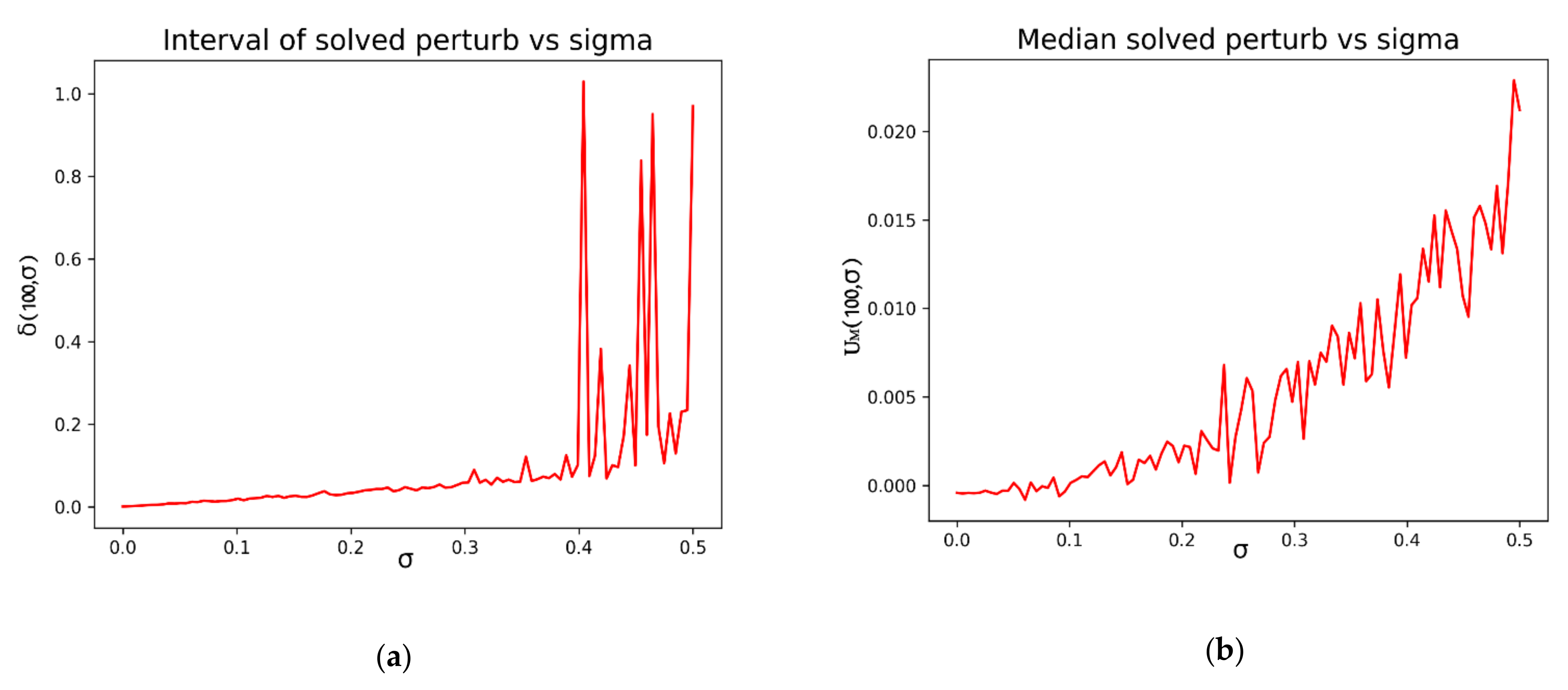
First, we can study the influence of the standard deviation parameter of the perturbation with respect to the differences between the extreme values $\delta \left(100,\sigma \right)$. It is also interesting to compare the evolution of $U_M\left(100,\sigma \right)$ with respect to the standard deviation. Those results can be seen in Figure 2a,b:

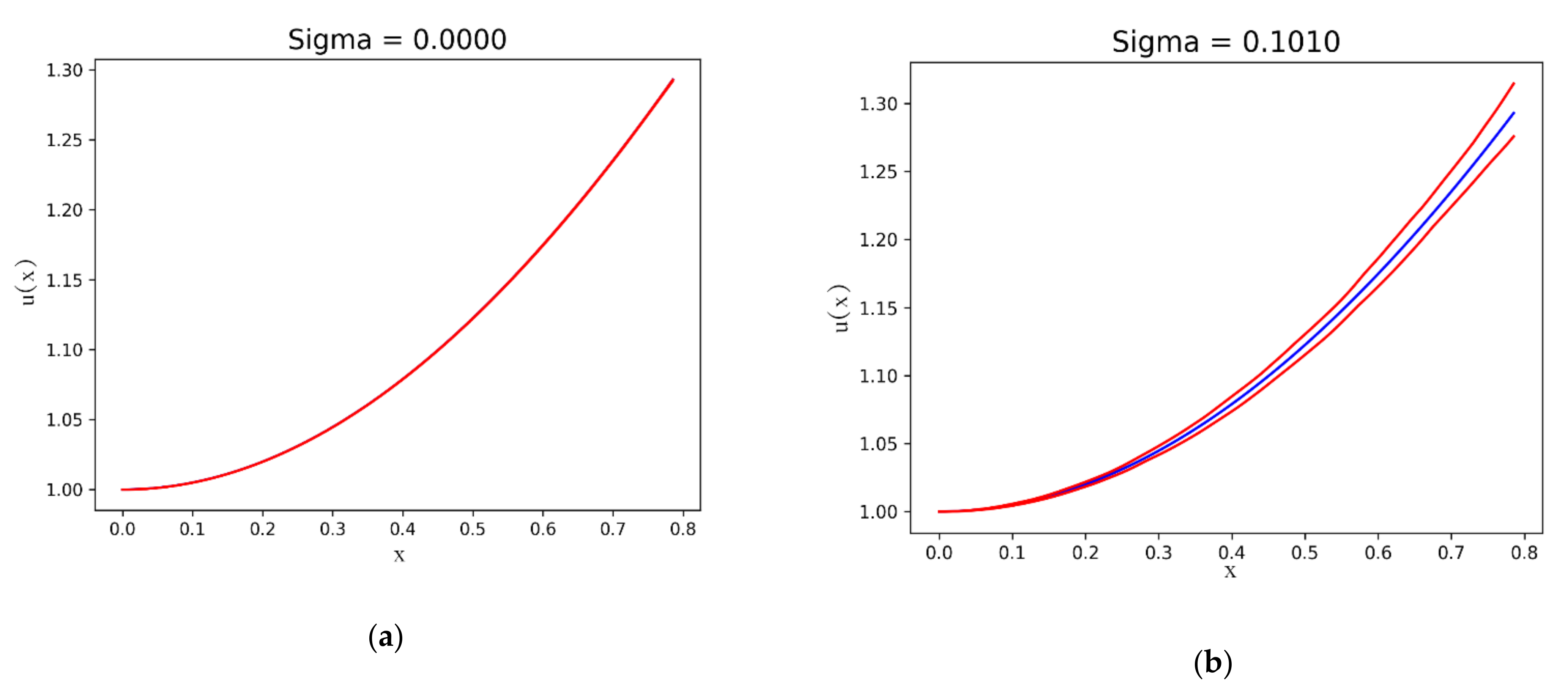
Figure 3 shows the exact $u\left(x\right)$ and the maximum $\overline{U}\left(x,n,\sigma \right)$ and minimum $\underset{\_}{U}\left(x,n,\sigma \right)$ of the numerical solutions at each point on for the iterations corresponding to different values of the standard deviation on the normal perturbation term:

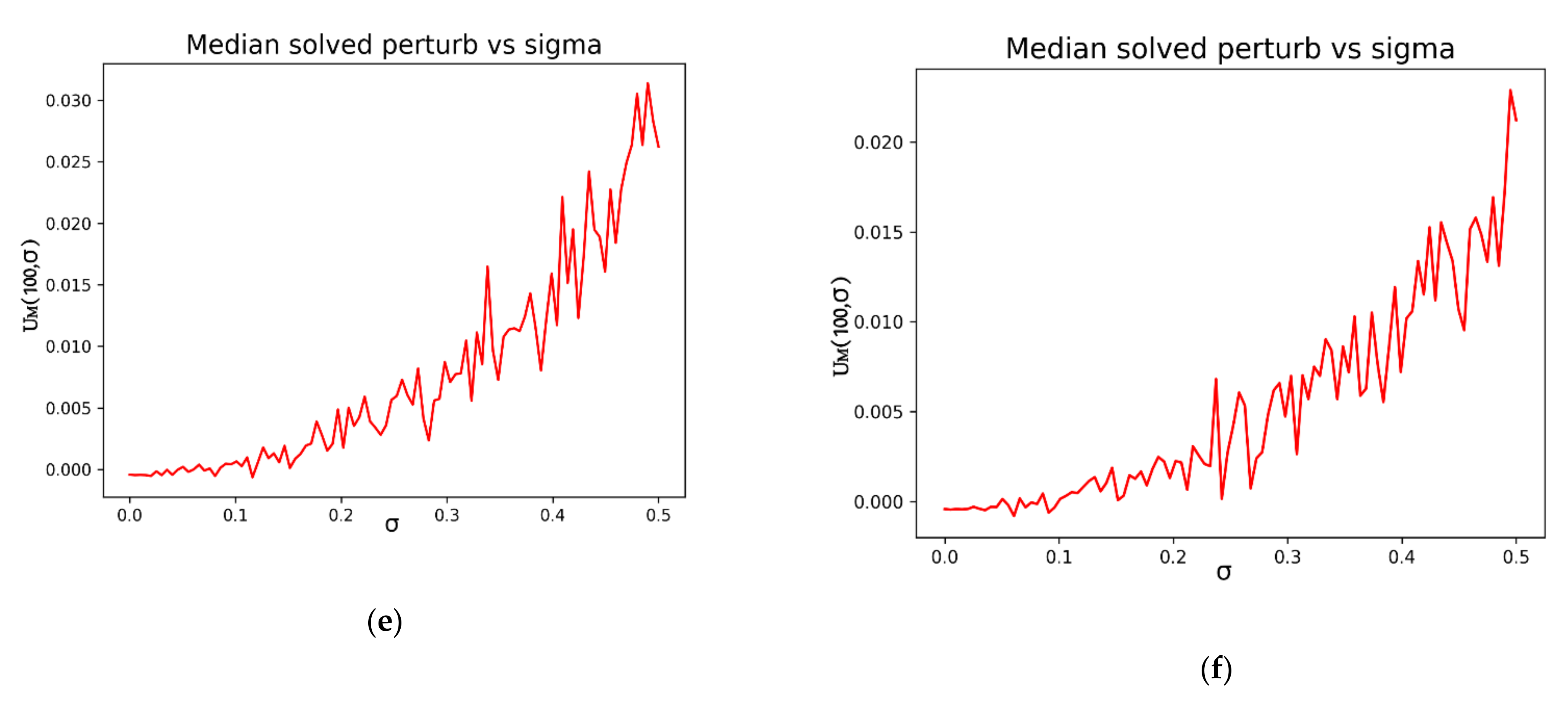
The dependence of the numerical solutions on the sample size can also be considered in order to study the algorithm efficiency. Figure 4 shows the same information that has been presented in Figure 2b for different sample sizes, from 5 to 100.

Table 1. Model parameters for the Example 1.

Sample Size	Std. Dev.	Iterations
100	0–0.5	200
5–100 1	0–0.5	200

¹ Results in Figure 4.

Table 1. Model parameters for the Example 1.

Sample Size	Std. Dev.	Iterations
100	0–0.5	200
5–100 1	0–0.5	200

¹ Results in Figure 4.

In general, the behavior is as expected, obtaining better accuracies as the number of points in the sample increases. However, it can be seen in Figure 4 how, for very small values of P, the result does not present a completely determinate behavior.

3.1.2. Example 2a

Another case of Equation (36) is:

$$\frac{d}{dx}\left(J_n\left(x\right)·\frac{du}{dx}\right)=J_m\left(x\right),$$

(38)

where:

$$J_m\left(x\right)=x^m·e^x.$$

(39)

The exact solution of this ODE can be obtained as:

$$u\left(x\right)=\int \frac{I_m\left(x\right)}{J_n\left(x\right)}dx=x^{m-n}-m·\int \frac{I_{m-1}\left(x\right)}{J_n\left(x\right)}dx,$$

(40)

where:

$$I_m\left(x\right)=\int J_m\left(x\right) dx.$$

(41)

The next two examples will allow comparing the results corresponding to the solutions of the different members of the family of parametric functions $J_n\left(x\right)$.

The first case corresponds with the values of the parameters given by $m=2$ and $n=4$. Let us study the solution $u\left(x\right)$ on the interval $\left[1,2\right]$ for the initial conditions $u\left(1\right)=-2/3$ and $u^{\prime }\left(1\right)=1$. The exact solution for the last equation is $u\left(x\right)=-\frac{1}{x}+\frac{1}{x^2}-\frac{2}{3}·\frac{1}{x^3}$.

Table 2. Model parameters for the Example 2a.

Sample Size	Std. Dev.	Iterations
100	0–0.5	200

Table 2. Model parameters for the Example 2a.

Sample Size	Std. Dev.	Iterations
100	0–0.5	200

Figure 5 shows the result for the equation given by $m=2$ and $n=4$.

In Figure 6 $\left(x\right)$, $\overline{U}\left(x,100,\sigma \right)$ and $\underset{\_}{U}\left(x,100,\sigma \right)$ are shown.

3.1.3. Example 2b

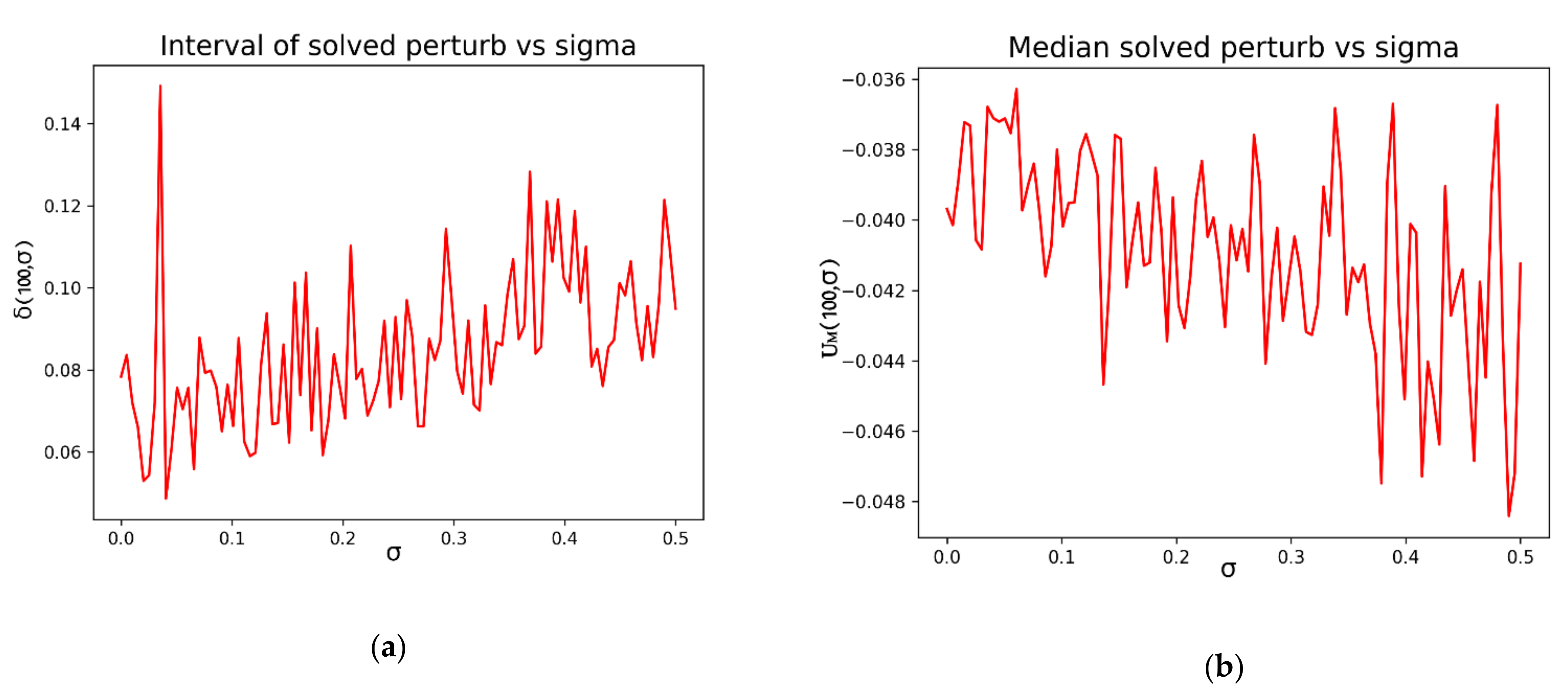
Example 2b corresponds to $m=3$ and $n=6$ on the interval $\left[1,2\right]$, with initial conditions $u\left(1\right)=1/5$ and $u^{\prime }\left(1\right)=-2$. In this case, the exact solution is given by the function $u\left(x\right)=-\frac{1}{2x^2}+\frac{1}{x^3}-\frac{3}{2x^4}+\frac{6}{5x^5}$. Figure 7 shows the difference $\delta \left(100,\sigma \right)$ and the median $U_M\left(100,\sigma \right)$.

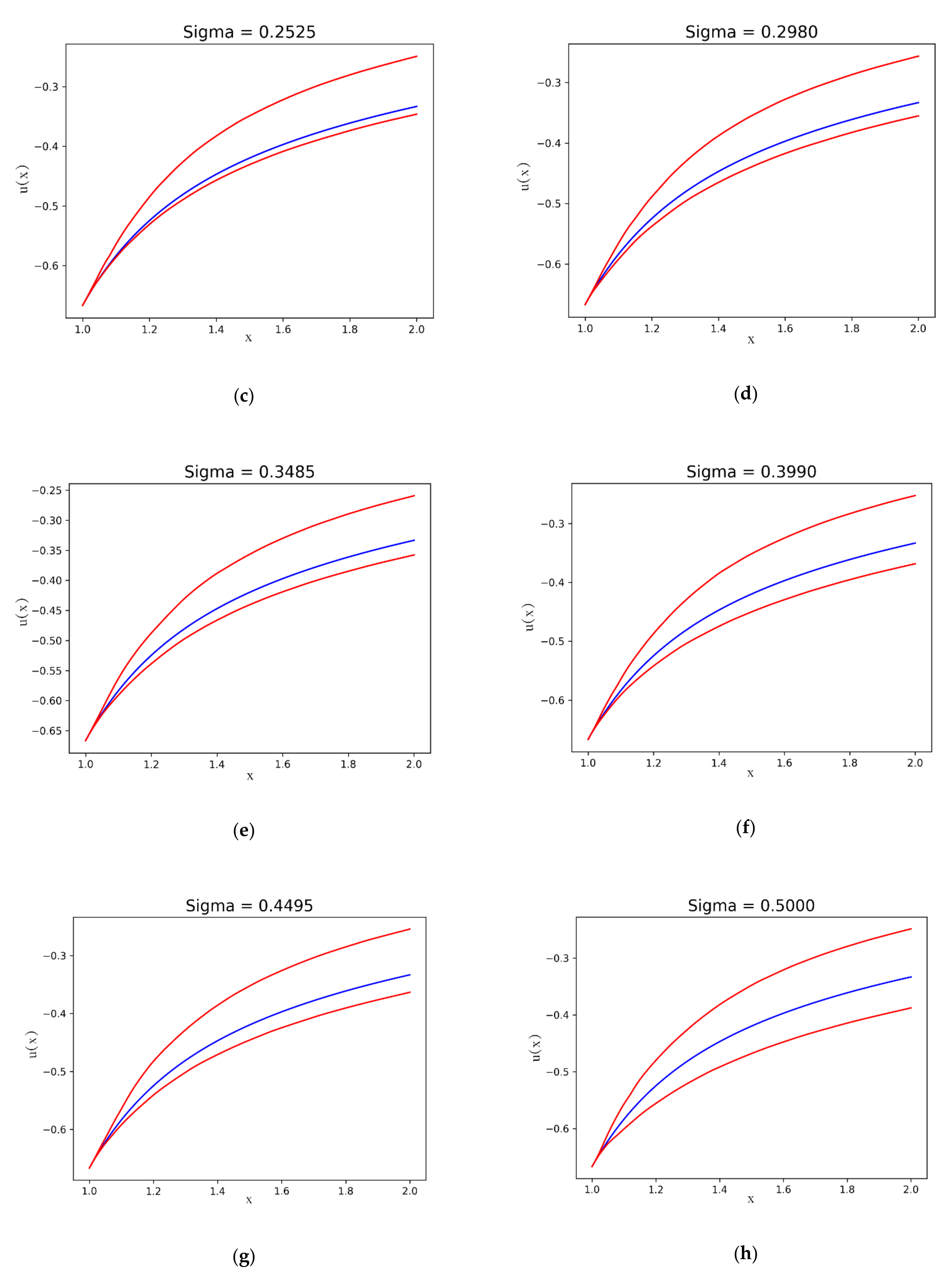
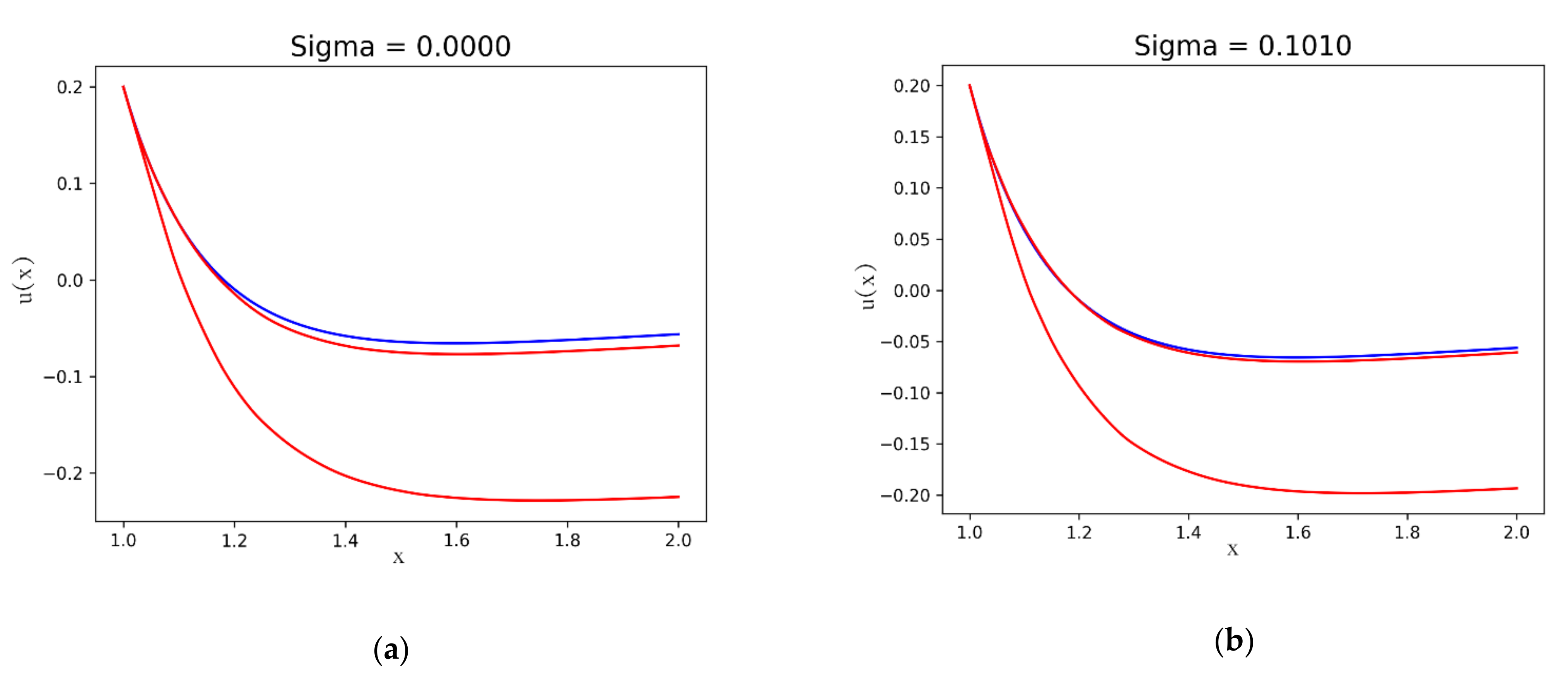
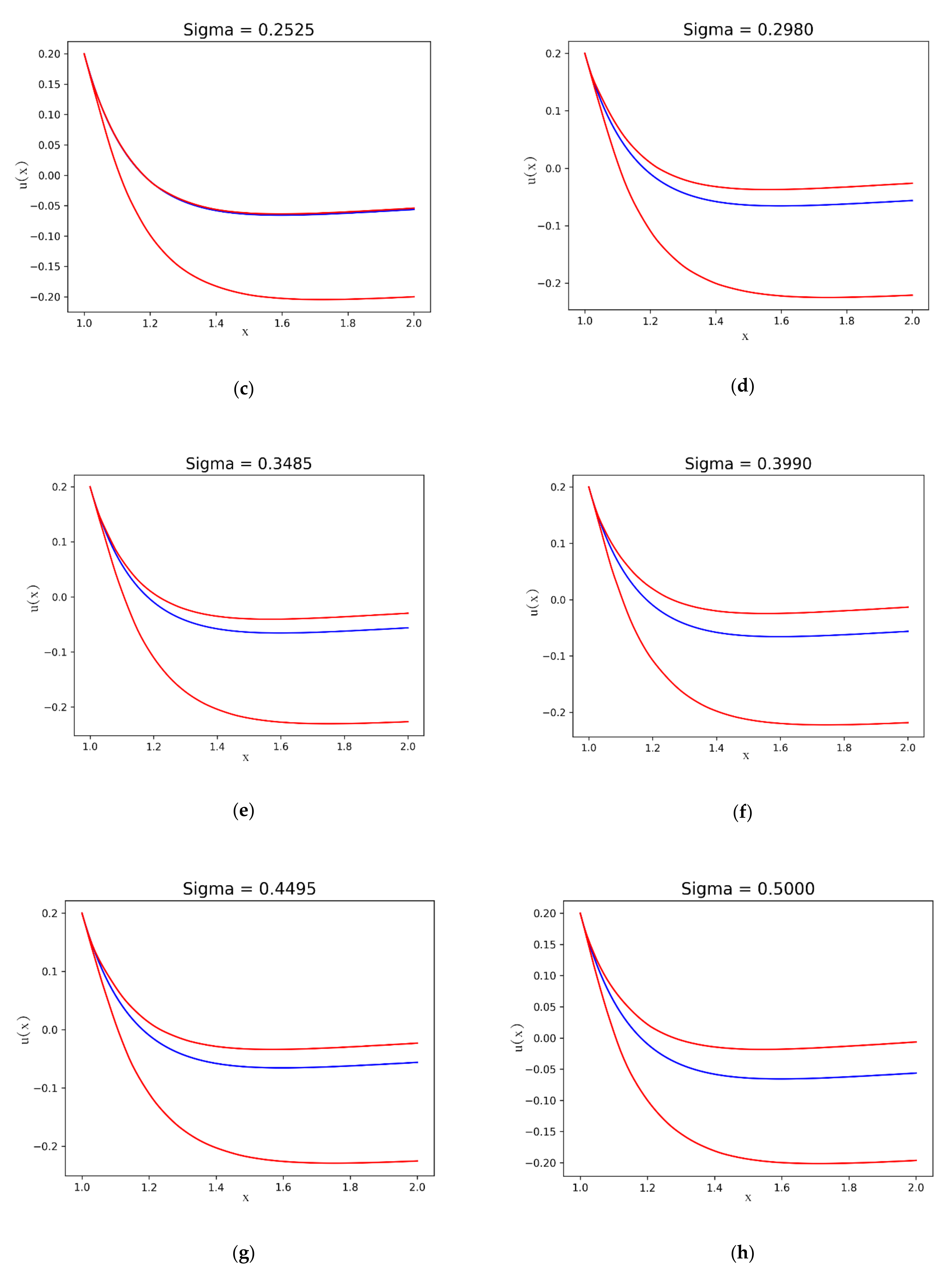
Figure 8 shows the exact and the maximum and minimum numerical solutions for the iterations corresponding to different values of the standard deviation on the normal perturbation term.

Figure 9 presents the effect of sample size on the solution error for sample sizes between 5 and 100 points.

Table 3. Model parameters for theExample 2b.

Sample Size	Std. Dev.	Iterations
100	0–0.5	200
5–100 1	0–0.5	200

¹ Results in Figure 9.

Table 3. Model parameters for theExample 2b.

Sample Size	Std. Dev.	Iterations
100	0–0.5	200
5–100 1	0–0.5	200

¹ Results in Figure 9.

3.2. Bass Equation. Example 3

The third example is a variation of a normalized Bass equation [37] with non-constant coefficients of innovation and imitation:

$$\frac{y^{\prime }\left(t\right)}{1-y\left(t\right)}=p\left(t\right)+q\left(t\right)·y\left(t\right),$$

(42)

defined over an interval $\left[0,5\right]$ with the initial condition given by $y\left(0\right)=0$. Typical values for the constants in Equation (42), are $p\sim 0.2\pm 0.1$ and $q\sim 0.4\pm 0.1$ [38]. In the studied example, two expressions are proposed. For the innovation coefficient:

$$p\left(t\right)=0.2·e^{-\frac{t}{2}},$$

(43)

and for the imitation coefficient:

$$q\left(t\right)=0.5·\left[t-{\left(\frac{t}{2}\right)}^2\right].$$

(44)

Table 4. Model parameters for the Example 3.

Sample Size	Std. Dev.	Iterations
100	0–0.5	200

Table 4. Model parameters for the Example 3.

Sample Size	Std. Dev.	Iterations
100	0–0.5	200

Figure 10 represents the parameters $\delta \left(100,\sigma \right)$ calculated with 200 different samples of the normal perturbation depending on the values of $\sigma$.

Figure 11 shows the difference between the exact and the maximum and minimum numerical solutions for the iterations corresponding to different values of the standard deviation on the normal perturbation term.

In order to facilitate the comparison between the different results, Figure 12 shows together some of the curves represented in Figure 11 for a different execution and function samples.

4. Discussion

In this research, the authors present a methodology for the modeling of differential equations and their resolution in systems where the functional expression of the functional parameters present in these equations is unknown and only an experimental sample of data is available. In the scientific literature, there are references to the determination of parameters of the differential equations governing a system by means of nonlinear regression on experimental data of the solution of the equation under study. Likewise, the field of study of differential equations for which the parameters follow a given distribution constitutes a fertile field of research.

The proposal developed focuses on considering equations whose parameters are unknown functions and whose values are deterministically determined, although affected by some type of error or perturbation. The algorithm allows obtaining numerical solutions for these equations by performing a previous numerical model of the functions involved from the experimental data.

Three different examples have been considered, two of them with known analytical solutions and another one considering only the numerical solution. From the study of the results obtained, it can be verified that the result of the algorithm shows behavior in accordance with what is expected with respect to the magnitude of the perturbation and the size of the experimental sample used to perform the modeling. On the other hand, the results show how the proposed methodology obtains solutions with a stable response to the corresponding perturbations.

From the present work, the main lines of future research would be two. On the one hand, the modification of the algorithm for the treatment of partial differential equations (PDE). On the other hand, it is worth investigating how to modify the design of the resolution algorithm to make it more computationally efficient. The way to do this would be to study how to combine the modeling algorithm with the resolution algorithm, minimizing the number of operations and the need for storage of the total program.