Bayes Synthesis of Linear Nonstationary Stochastic Systems by Wavelet Canonical Expansions

Abstract

This article is devoted to analysis and optimization problems of stochastic systems based on wavelet canonical expansions. Basic new results: (i) for general Bayes criteria, a method of synthesized methodological support and a software tool for nonstationary normal (Gaussian) linear observable stochastic systems by Haar wavelet canonical expansions are presented; (ii) a method of synthesis of a linear optimal observable system for criterion of the maximal probability that a signal will not exceed a particular value in absolute magnitude is given. Applications: wavelet model building of essentially nonstationary stochastic processes and parameters calibration.

1. Introduction

Nowadays, for stochastic systems research, e.g., functioning at essentially nonstationary disturbances of complex structures, we need analytical modeling technologies for accurate analysis and synthesis. Methods of analysis and synthesis based on canonical expansions are very suitable for quick analytical modeling realizations using the first two probabilistic moments. Wavelet canonical expansions essentially increase the flexibility and accuracy of corresponding technologies.

It is known [1,2,3] that canonical expansion (CE) of stochastic processes (StP) is widely used to solve problems of analysis, modeling and synthesis of linear nonstationary stochastic systems (StS). For StS with high availability, corresponding software tools based on CE were worked out in [4,5,6,7,8]. In [4], we gave a brief review of the known algorithmic and software tools. In [5,6], the issues of instrumental software for analytical modeling of nonstationary scalar and vector random functions by means of wavelet CE (WLCE) are considered. The parameters of WLCE are expressed in terms of the coefficients of the expansion of the covariance matrix of random function over two-dimensional Dobshy wavelets. Article [7] continues the thematic cycle dedicated to analytical modeling of linear nonstationary StS based on wavelet and wavelet canonical expansions. The article describes wavelet algorithms for analytical modeling of mathematical expectation, a covariance matrix and a matrix of covariance functions, as well as wavelet algorithms for spectral and correlation-analytical express modeling.

The article [8] continues the thematic cycle devoted to software tools for analytical modeling of linear with parametric interference (Gaussian and non-Gaussian) StS based on nonlinear correlation theory (the method of normal approximation and the method of canonical expansions). Analytical methods are based on orthogonal decomposition of covariance matrix elements using a two–dimensional Dobshy wavelet with a compact carrier and Galerkin–Petrov wavelet methods.

In [5], for an essentially nonstationary StP wavelet, CE (WLCE) was proposed. Nowadays, deterministic wavelet methods are intensively applied to the problems of numerical analysis and modeling. A broad class of numerical methods based on Haar wavelets achieved great success [9]. These methods are simple in the sense of versatility and flexibility and possess less computational cost for accuracy analysis problems. The theory and practice of wavelets has attained its modern growth due to mathematical analysis of the wavelet in [10,11,12]. The concept of multiresolution analysis was given in [13]. In [14,15] method to construct wavelets with compact support and scaling function was developed. Among the wavelet families, which are described by an analytical expression, the Haar wavelets deserve special attention. Haar wavelets, in combination with the Galerkin method, are very effective and popular for solving different classes of deterministic equations [16,17,18,19,20,21,22,23,24,25]. The application of a wavelet for CE of StP and stochastic differential and integrodifferential equations was given in [7,8,26].

In [27,28], design problems for linear mean square (MS) optimal filters are considered on the basis of WLCE. Explicit formulae for calculating the MS optimal estimate of the signal and the MS optimal estimate of the quality of the constructed linear MS optimal operator are derived. Articles [29,30] are devoted to the synthesis of wavelets in accordance with complex statistical criteria (CsC). The basic definitions of CsC and approaches are given. Methodological support is based on Haar wavelets. The main wavelet equations, algorithms, software tools and examples are given. Some particular aspects of the StS wavelet synthesis under nonstationary (for example, shock) perturbations are presented in [31].

The developed wavelet algorithms have a fairly high degree of versatility and can be used in various applied fields of science. Such complex StS describes organizations–technical–economical systems functioning in the presence of internal and external noises and stochastic factors. The developed wavelet algorithms are used for data analysis and information processing in high-availability stochastic systems, in complex data storage systems, model building and calibration.

Let us state the general problem of the Bayes synthesis of linear nonstationary normal observable StS (OStS) by WLCE means. Special attention will be paid to the synthesis of linear optimal system for criterion of the maximum probability that the signal will not exceed a particular value in absolute magnitude. For example, the results of computer experiments are presented and discussed.

2. Bayes Criteria

In practice [1,2], the choice of criterion for comparing alternative systems for the same purpose, like any question regarding the choice of criteria, is largely a matter of common sense, which can often be approached from consideration of operating conditions and purpose of any particular system.

The criterion of the maximum probability that the signal will not exceed a particular value in absolute magnitude can be represented as

$$E[l(W,W^{*})]=\min .$$

(1)

If we take the function $l$ as the characteristic function of the corresponding set of values of the error, the following formula is valid:

$$l(W,W^{*})=\{\begin{array}{l}1\hspace{1em}\mathrm{at}\hspace{1em}|W^{*}-W|>W,\\ 0\hspace{1em}\mathrm{at}\hspace{1em}|W^{*}-W|\le W.\end{array}$$

(2)

In applications connected with damage accumulation (1) needs to be employed with function $l$ in the form:

$$l(W,W^{*})=1-e^{-k^2{(W^{*}-W)}^2}.$$

(3)

Thus, we get the following general principle for estimating the quality of a system and selecting the criterion of optimality. The quality of the solution of the problem in each actual case is estimated by a function $l(W,W^{*})$, the value of which is determined by the actual realizations of the signal $W$ and its estimator $W^{*}$. It is expedient to call this the loss function. The quality of the solution of the problem on average for a given realization of the signal $W$ with all possible realizations of the estimator $W^{*}$ corresponding to particular realization of the signal $W$ is estimated by the conditional mathematical expectation of the loss function for the given realization of the signal:

$$\rho (A|W)=E[l(W,W^{*}|W)].$$

(4)

This quantity is called conditional risk. The conditional risk depends on the operator $A$ for the estimator $W^{*}$ and on the realization of signal $W$. Finally, the average quality of the solution for all possible realization of $W$ and its estimator $W^{*}$ is characterized by the mathematical expectation of the conditional risk

$$\mathrm{R}(A)=E[\rho (A|W)|W]=E[l(W,W^{*})].$$

(5)

This quantity is called the mean risk.

All criteria of minimum risk which correspond to the possible loss functions or functionals which may contain undetermined parameters are known as Bayes’ criteria.

3. Basic formulae for Optimal Bayes Synthesis of Linear Systems

Let us consider scalar linear OStS with real StP $Z(\tau )$ $\left(\tau \in [t-T,t]\right)$, which is the sum of the useful signal and the additive normal noise $X(\tau )$:

$$Z(\tau )={\displaystyle \sum _{r=1}^N{U}_r}{\xi }_r(\tau )+X(\tau ).$$

(6)

The useful signal is the linear combination of given random parameters $U_r^{}\hspace{1em}(r=\overline{1,N})$. We need to get StP $W(t)$ in the following form:

$$W(t)={\displaystyle \sum _{r=1}^N{U}_r}{\zeta }_r(t)+Y(t).$$

(7)

Here, ${\xi }_1(\tau ),\dots ,{\xi }_N(\tau ),{\zeta }_1(\tau ),\dots ,{\zeta }_N(\tau )$ are known structural functions; $U_1,\dots ,U_N$ are given random variables (RV) which do not depend on noises $X(\tau ),\hspace{0.17em}Y(\tau )$ $(EX(\tau )=0,$ $EY(\tau )=0)$.

We state to construct an optimal system with operator $A$ in cases when output StP:

$$W^{*}(t)=AZ$$

(8)

based on observation StP $Z(\tau )$ at time interval $[t-T,t]$, reproducing given output signal $W(t)$ for criteria (1) with maximal accuracy.

It is known [1,2,3] that the solution of this problem through CE is based on two-stage procedures based on Formulae (4) and (5).

Vector CE ${\left[\begin{array}{cc}X(\tau )& Y(\tau )\end{array}\right]}^T$ presents the linear combination of uncorrelated RV with deterministic coordinate functions:

$$X(\tau )={\displaystyle \sum _{\nu }{V}_{\nu }}{x}_{\nu }(\tau ),\hspace{1em}Y(\tau )={\displaystyle \sum _{\nu }{V}_{\nu }}{y}_{\nu }(\tau )$$

(9)

According to [1,2] for $V_{\nu }$ we have

$$V_{\nu }={\displaystyle \underset{t-T}{\overset{t}{\int }}{a}_{\nu }^{}(\tau )X(\tau )d\tau }+{\displaystyle \underset{t-T}{\overset{t}{\int }}{a}_{\nu }^{}(\tau )Y(\tau )d\tau }$$

(10)

Then, coordinate functions are calculated by the following formulae:

$$x_{\nu }(\tau )=\frac{1}{D_{\nu }}{\displaystyle \underset{t-T}{\overset{t}{\int }}{a}_{\nu }^{}(\theta )K_X(\tau ,\theta )d\theta }+\frac{1}{D_{\nu }}{\displaystyle \underset{t-T}{\overset{t}{\int }}{a}_{\nu }^{}(\theta )K_{XY}(\tau ,\theta )d\theta },$$

(11)

$$y_{\nu }(\tau )=\frac{1}{D_{\nu }}{\displaystyle \underset{t-T}{\overset{t}{\int }}{a}_{\nu }^{}(\theta )K_{XY}(\theta ,\tau )d\theta +\frac{1}{D_{\nu }}{\displaystyle \underset{t-T}{\overset{s}{\int }}{a}_{\nu }^{}(\theta )K_Y(\tau ,\theta )d\theta }}.$$

(12)

Here, $E\left[V_{\nu }\right]=0.$ $D_{\nu }=D\left[V_{\nu }\right],$ $K_X(\tau ,\theta )=E\left[X(\tau )\cdot X(\theta )\right],$ $K_{XY}(\tau ,\theta )=E\left[X(\tau )\cdot Y(\theta )\right],$ $K_Y(\tau ,\theta )=E\left[Y(\tau )\cdot Y(\theta )\right];$ $a_{\nu }^{}(\tau )$ is a given set of deterministic functions satisfying biorthogonality conditions:

$${\displaystyle \underset{t-T}{\overset{t}{\int }}{a}_{\nu }^{}(\tau )x_{\mu }(\tau )d\tau }+{\displaystyle \underset{t-T}{\overset{t}{\int }}{a}_{\nu }^{}(\tau )y_{\mu }(\tau )d\tau }={\delta }_{\nu \mu }.$$

(13)

Let us consider RV

$$Z_{\nu }={\displaystyle \underset{t-T}{\overset{t}{\int }}{a}_{\nu }^{}(\tau )Z(\tau )d\tau ,}$$

(14)

and its presentation

$$Z_{\nu }={\displaystyle \sum _{r=1}^N{\alpha }_{\nu r}{U}_r+V_{\nu },}$$

(15)

where

$${\alpha }_{\nu r}={\displaystyle \underset{t-T}{\overset{t}{\int }}{a}_{\nu }^{}(\tau ){\xi }_r(\tau )d\tau }.$$

(16)

The sum of RV $Z_{\nu }$, multiplied by $x_{\nu }(\tau )$ gives the CE of StP $Z(\tau )\hspace{1em}(\tau \in \left[t-T,t\right])$

$$Z(\tau )={\displaystyle \sum _{\nu }^{}{Z}_{\nu }}{x}_{\nu }(\tau ).$$

(17)

To find the conditional mathematical expectation of the loss function for StP $Z(\tau )\hspace{1em}(\tau \in \left[t-T,t\right])$, it is necessary to find the conditional probability density of output StP relatively on input StP $Z(\tau )$. According to (4), StP $W(t)$ depends upon the given random parameters $U_r\hspace{1em}(r=\overline{1,N})$ and random noise $Y(t)$. So, we get

$$Y(t)={\displaystyle \sum _{\nu }{V}_{\nu }}{y}_{\nu }(t)={\displaystyle \sum _{\nu }\left(Z_{\nu }-{\displaystyle \sum _{r=1}^N{\alpha }_{\nu r}{U}_r}\right)}{y}_{\nu }(t)={\displaystyle \sum _{\nu }{Z}_{\nu }}{y}_{\nu }(t)-{\displaystyle \sum _{r=1}^N{U}_r}{\displaystyle \sum _{\nu }{\alpha }_{\nu r}}{y}_{\nu }(t).$$

(18)

Here,

$$W(t)={\displaystyle \sum _{r=1}^N{U}_r}{\zeta }_r(t)+{\displaystyle \sum _{\nu }{Z}_{\nu }}{y}_{\nu }(t)-{\displaystyle \sum _{r=1}^N{U}_r}{\displaystyle \sum _{\nu }{\alpha }_{\nu r}}{y}_{\nu }(t).$$

(19)

The last formula shows that StP $W(t)$ depends upon random parameters $U_r\hspace{0.17em}\hspace{1em}(r=\overline{1,N})$ and the set of $Z_{\nu }$.

Let us introduce the vector of RV $U={\left[\begin{array}{cccc}{U}_1& U_2& \dots & U_N\end{array}\right]}^T$. Conditional distribution of $U$ relative StP $Z(\tau )$ coincides with the set of RV $Z_{\nu }\hspace{0.17em}$. Conditional density $f_1(u|z_1,z_2,\dots )$ is defined by the known formula:

$$f_1(u|z_1,z_2,\dots )=\frac{f(u)f_2(z_1,z_2,\dots |u)}{{\displaystyle \underset{-\infty }{\overset{+\infty }{\int }}f(u)f_2(z_1,z_2,\dots |u)du}}.$$

(20)

Here, $f(u)$ is a given apriority density of RV $U={\left[\begin{array}{cccc}{U}_1& U_2& \dots & U_N\end{array}\right]}^T$; $f_2(z_1,z_2,\dots |u)$ is a density of RV $Z_{\nu }\hspace{0.17em}$, relatively $U={\left[\begin{array}{cccc}{U}_1& U_2& \dots & U_N\end{array}\right]}^T$.

Taking into account that vector random noise is normal, $V_{\nu }\hspace{0.17em}$ is the linear transform of vector ${\left[\begin{array}{cc}X(\tau )& Y(\tau )\end{array}\right]}^T$. We conclude that RV are not only correlated, but also independent. Joint density of $V_{\nu }\hspace{0.17em}$ with zero mathematical exactions and variances $D_{\nu }\hspace{0.17em}$ is expressed by formula

$$f_V(v_1,v_2,\dots )=\frac{1}{\sqrt{{\left(2\pi \right)}^L{D}_1\cdot D_2\cdot \dots }}\exp \left\{-\frac{1}{2}{\displaystyle \sum _{\nu }^{}\frac{v_{\nu }^2}{D_{\nu }}}\right\}.$$

(21)

In (7), let us replace RV $U_1,\dots ,U_N$ with their realizations $u_1,\dots ,u_N$; then, $Z_{\nu }\hspace{0.17em}$ is the linear function of RV $V_{\nu }\hspace{0.17em}$ with known joint density. Expressing $V_{\nu }\hspace{0.17em}$ by $Z_{\nu }\hspace{0.17em}$ and using Formula (21), we get:

$$f_2(z_1,z_2,\dots |u)=\frac{1}{\sqrt{{\left(2\pi \right)}^L{D}_1\cdot D_2\cdot \dots }}\exp \left\{-\frac{1}{2}{\displaystyle \sum _{\nu }^{}\frac{1}{D_{\nu }}{\left(z_{\nu }-{\displaystyle \sum _{r=1}^N{\alpha }_{\nu r}{u}_r}\right)}^2}\right\},$$

(22)

where ${\alpha }_{\nu }(u)={\displaystyle \sum _{r=1}^N{\alpha }_{\nu r}{u}_r}$.

After substituting Formula (22) into (20), we get the formula for a posteriori density $f_1(u|z_1,z_2,\dots )$ of $U={\left[\begin{array}{cccc}{U}_1& U_2& \dots & U_N\end{array}\right]}^T$ for input StP $Z(\tau )$ $(\tau \in [t-T,t])$:

$$f_1(u|z_1,z_2,\dots )=\chi (z)f(u)\exp \left\{{\displaystyle \sum _{\nu }^{}\frac{z_{\nu }{\alpha }_{\nu }(u)}{D_{\nu }}}-\frac{1}{2}{\displaystyle \sum _{\nu }^{}\frac{{\alpha }_{\nu }^2(u)}{D_{\nu }}}\right\},$$

(23)

$$\chi (z)={\left[{\displaystyle \underset{-\infty }{\overset{+\infty }{\int }}f(u)\exp \left\{{\displaystyle \sum _{\nu }^{}\frac{z_{\nu }{\alpha }_{\nu }(u)}{D_{\nu }}}-\frac{1}{2}{\displaystyle \sum _{\nu }^{}\frac{{\alpha }_{\nu }^2(u)}{D_{\nu }}}\right\}du}\right]}^{-1}.$$

(24)

This formula may be used after observation when realization $Z(\tau )$ is available.

A posteriori mathematical expectation of loss function $l(W,W^{*})$ is called conditional risk, and is denoted as $\rho (A|W)$:

$$\begin{array}{l}\rho (A|W)=E\left[l\left(W,W^{*}\right)|Z\right]=\chi (z){\displaystyle \underset{-\infty }{\overset{+\infty }{\int }}l\left(W,W^{*}\right)}f(u)\\ \times \exp \left\{{\displaystyle \sum _{\nu }^{}\frac{z_{\nu }{\alpha }_{\nu }(u)}{D_{\nu }}}-\frac{1}{2}{\displaystyle \sum _{\nu }^{}\frac{{\alpha }_{\nu }^2(u)}{D_{\nu }}}\right\}du.\end{array}$$

(25)

In order to solve the stated problem, it is necessary to calculate the optimal output StP $W^{*}(t)$ for every $t$ from condition of minimum of integral (11).

Let us consider this integral as a function of ${{\rm P}}^W=W^{*}(t)$ at fixed values of parameters

$${\eta }_0={\eta }_0(z_1,z_2,\dots )={\displaystyle \sum _{\nu }^{}{z}_{\nu }{y}_{\nu }(t)},\hspace{1em}{\eta }_r={\eta }_r(z_1,z_2,\dots )={\displaystyle \sum _{\nu }^{}\frac{{\alpha }_{\nu r}{z}_{\nu }}{D_{\nu }}}\hspace{0.17em}\hspace{1em}(r=\overline{1,N})$$

(26)

and time $t$:

$$\begin{array}{l}I({{\rm P}}^W,{\eta }_1,\dots ,{\eta }_N,t)={\displaystyle \underset{-\infty }{\overset{+\infty }{\int }}\dots {\displaystyle \underset{-\infty }{\overset{+\infty }{\int }}l\left({\displaystyle \sum _{r=1}^N{u}_r}\left({\zeta }_r(t)-b_{r0}\right)+{\eta }_0,{{\rm P}}^W\right)}}f(u_1,\dots ,u_N)\\ \times \exp \left\{{\displaystyle \sum _{r=1}^N{\eta }_r{u}_r}-\frac{1}{2}{\displaystyle \sum _{p,q=1}^N{b}_{pq}{u}_p{u}_q}\right\}d{u}_1\dots d{u}_N.\end{array}$$

(27)

Here,

$$b_{p0}={\displaystyle \sum _{\nu }^{}{\alpha }_{\nu p}{y}_{\nu }(t)},\hspace{0.17em}\hspace{1em}{b}_{pq}={\displaystyle \sum _{\nu }^{}\frac{1}{D_{\nu }}{\alpha }_{\nu p}{\alpha }_{\nu q}}\hspace{0.17em}\hspace{1em}(q,p=\overline{1,N}).$$

(28)

The value of parameter ${{\rm P}}^W={{\rm P}}_0^W(t,{\eta }_0,{\eta }_1,\dots ,{\eta }_N)$ when integral (27) reaches the minimum value defines the Bayes optimal operator for criterion (1). Changing ${\eta }_r\hspace{0.17em}(r=\overline{0,N})$ and ${{\rm P}}_0^W(t,{\eta }_0,\dots ,{\eta }_N)$ variables ${\eta }_1,\dots ,{\eta }_N$ and $z_1,z_2,\dots$ with the corresponding RV ${\mathrm{H}}_0,\dots ,{\mathrm{H}}_N$ and $Z_1,Z_2,\dots$, we get the required optimal operator:

$$W^{*}(t)=AZ={{\rm P}}_0^w(t,{\mathrm{H}}_0,\dots ,{\mathrm{H}}_N),$$

(29)

where

$${\mathrm{H}}_0={\displaystyle \sum _{\nu }^{}{Z}_{\nu }{y}_{\nu }(t)},\hspace{1em}{\mathrm{H}}_r={\mathrm{H}}_r(Z_1,Z_2,\dots )={\displaystyle \sum _{\nu }^{}\frac{{\alpha }_{\nu r}{Z}_{\nu }}{D_{\nu }}}\hspace{0.17em}\hspace{1em}(r=\overline{1,N})$$

(30)

The quality of the optimal operator is estimated by the mean risk [1,2]

$$\begin{array}{l}R(A)=E\left[\rho (A|W)|W\right]=E\left[l\left(W,W^{*}\right)\right]\\ ={\displaystyle \underset{-\infty }{\overset{+\infty }{\int }}\dots {\displaystyle \underset{-\infty }{\overset{+\infty }{\int }}l\left({\displaystyle \sum _{r=1}^N{u}_r}\left({\zeta }_r(t)-b_{r0}\right)+{\eta }_0,{{\rm P}}_0^W\right)}}{f}_2(z_1,z_2,\dots |u)f(u)d{z}_{1}d{z}_2\dots du.\end{array}$$

(31)

So, we get the following basic Formulae (23)–(31) necessary for wavelet canonical expansion method.

4. Wavelet Canonical Expansions Method

Let us construct an operator for an optimal linear system using the Haar wavelet CE method WLCE [5,6]:

$$\left\{{\phi }_{00}^{}(\overline{\tau }),\hspace{0.17em}\hspace{0.17em}{\psi }_{jk}^{}(\overline{\tau })\right\}$$

(32)

where

$${\phi }_{00}^{}(\overline{\tau })\hspace{0.17em}=\hspace{0.17em}\phi (\overline{\tau })=\{\begin{array}{c}1,\hspace{0.17em}\overline{\tau }\in \left[0,1\right),\\ 0,\overline{\tau }\notin \left[0,1\right)\end{array} \mathrm{is} \mathrm{a} \mathrm{scaling} \mathrm{function},$$

(33)

$${\psi }_{00}^{}(\overline{\tau })\hspace{0.17em}=\hspace{0.17em}\psi (\overline{\tau })=\{\begin{array}{c}1,\hspace{0.17em}\overline{\tau }\in \left[0,\frac{1}{2}\right),\\ -1,\overline{\tau }\in \left[\frac{1}{2},1\right),\hspace{0.17em}\\ 0,\hspace{0.17em}\tau \notin \left[0,1\right)\end{array} \mathrm{is} \mathrm{a} \mathrm{mother} \mathrm{wavelet},$$

(34)

${\psi }_{jk}^{}(\overline{\tau })\hspace{0.17em}=\hspace{0.17em}\sqrt{2^j}\psi (2^j\overline{\tau }-k)$ are wavelets of level $j$ for $j=1,2,\dots ,J;$ $k=0,1,\dots ,2^j-1;\hspace{0.17em}\hspace{0.17em}J$ is maximal resolution level defined by required accuracy of approximation for any function $f(\overline{\tau })\in \hspace{0.17em}{L}^2\left[0,1\right]$ by finite linear combination of Haar wavelets, equal to $2^{-\frac{J}{2}}$.

Then, let us present a one-dimensional wavelet basis (32) as:

$$\begin{array}{l}{g}_1(\overline{\tau })={\phi }_{00}^{}(\overline{\tau }),\hspace{0.17em}\hspace{1em}{g}_2(\overline{\tau })={\psi }_{00}^{}(\overline{\tau }),\hspace{1em}{g}_{\nu }(\overline{\tau })={\psi }_{jk}^{}(\overline{\tau }),\hspace{1em}\\ j=1,2,\dots ,J;\hspace{0.17em}\hspace{1em}k=0,1,\dots ,2^j-1;\hspace{0.17em}\hspace{1em}\nu =2^j+k+1;\hspace{0.17em}\hspace{1em}\nu =\overline{3,L.}\end{array}$$

(35)

For construction of the Haar WLCE for vector ${\left[\begin{array}{cc}X(\tau )& Y(\tau )\end{array}\right]}^T$ at $\tau \in \left[t-T,t\right]$, we pass to new time variable $\overline{\tau }\in \hspace{0.17em}\left[0,1\right]\hspace{0.17em},\hspace{0.17em}$ $\overline{\tau }=\frac{\tau -(t-T)}{T}$ and assume

$$\begin{array}{l}{K}_X({\tau }_1,{\tau }_2)\in L^2\left(\left[t-T,t\right]\times \left[t-T,t\right]\right),\hspace{1em}{K}_{XY}({\tau }_1,{\tau }_2)\in L^2\left(\left[t-T,t\right]\times \left[t-T,t\right]\right),\\ K_Y({\tau }_1,{\tau }_2)\in L^2\left(\left[t-T,t\right]\times \left[t-T,t\right]\right),\end{array}$$

(36)

$$\begin{array}{l}{\overline{K}}_X({\overline{\tau }}_1,{\overline{\tau }}_2)\in L^2\left(\left[0,1\right]\times \left[0,1\right]\right)\hspace{0.17em},\hspace{1em}{\overline{K}}_{XY}({\overline{\tau }}_1,{\overline{\tau }}_2)\in L^2\left(\left[0,1\right]\times \left[0,1\right]\right)\hspace{0.17em},\\ {\overline{K}}_Y({\overline{\tau }}_1,{\overline{\tau }}_2)\in L^2\left(\left[0,1\right]\times \left[0,1\right]\right)\hspace{0.17em}.\end{array}$$

(37)

Additionally, for presentation of given covariance functions in the form of two-dimensional wavelet expansion, it is necessary to define the two-dimensional orthogonal basis through tensor composition of one-dimensional bases (32) when scaling is performed simultaneously for two variables

$$\begin{array}{l}{\Phi }_{}^A({\overline{\tau }}_1,{\overline{\tau }}_2)\hspace{0.17em}=\hspace{0.17em}{\phi }_{00}^{}({\overline{\tau }}_1){\phi }_{00}^{}({\overline{\tau }}_2),\hspace{1em}{\Psi }_{}^{\mathrm{H}}({\overline{\tau }}_1,{\overline{\tau }}_2)\hspace{0.17em}=\hspace{0.17em}{\phi }_{00}^{}({\overline{\tau }}_1){\psi }_{00}^{}({\overline{\tau }}_2),\\ {\Psi }_{}^B({\overline{\tau }}_1,{\overline{\tau }}_2)\hspace{0.17em}=\hspace{0.17em}{\psi }_{00}^{}({\overline{\tau }}_1){\phi }_{00}^{}({\overline{\tau }}_2),\hspace{1em}{\Psi }_{jkn}^D({\overline{\tau }}_1,{\overline{\tau }}_2)\hspace{0.17em}=\hspace{0.17em}{\psi }_{jk}^{}({\overline{\tau }}_1){\psi }_{jn}^{}({\overline{\tau }}_2)\end{array}$$

(38)

where $j=1,2,\dots ,J;\hspace{0.17em}k,n=0,1,\dots ,2^j-1$.

So, the two-dimensional wavelet expansion of given covariance functions takes the form

$${\overline{K}}_X({\overline{\tau }}_1,{\overline{\tau }}_2)=\hspace{0.17em}{a}^x{\Phi }_{}^A({\overline{\tau }}_1,{\overline{\tau }}_2)+h_{}^x{\Psi }_{}^{\mathrm{H}}({\overline{\tau }}_1,{\overline{\tau }}_2)+b_{}^x{\Psi }_{}^B({\overline{\tau }}_1,{\overline{\tau }}_2)+{\displaystyle {\sum }_{j=0}^J{\displaystyle {\sum }_{k=0}^{2^J-1}{\displaystyle {\sum }_{n=0}^{2^J-1}{d}_{jkn}^x{\Psi }_{jkn}^D({\overline{\tau }}_1,{\overline{\tau }}_2)}}}$$

(39)

where

$$\begin{array}{l}{a}^x={\displaystyle \underset{0}{\overset{1}{\int }}{\displaystyle \underset{0}{\overset{1}{\int }}{\overline{K}}_X({\overline{\tau }}_1,{\overline{\tau }}_2)}}{\Phi }_{}^A({\overline{\tau }}_1,{\overline{\tau }}_2)d{\overline{\tau }}_{1}d{\overline{\tau }}_2,\hspace{1em}{h}_{}^x\hspace{0.17em}=\hspace{0.17em}{\displaystyle \underset{0}{\overset{1}{\int }}{\displaystyle \underset{0}{\overset{1}{\int }}{\overline{K}}_X({\overline{\tau }}_1,{\overline{\tau }}_2)}}{\Psi }_{}^{\mathrm{H}}({\overline{\tau }}_1,{\overline{\tau }}_2)d{\overline{\tau }}_{1}d{\overline{\tau }}_2,\\ b_{}^x\hspace{0.17em}=\hspace{0.17em}{\displaystyle \underset{0}{\overset{1}{\int }}{\displaystyle \underset{0}{\overset{1}{\int }}{\overline{K}}_X({\overline{\tau }}_1,{\overline{\tau }}_2)}}{\Psi }_{}^B({\overline{\tau }}_1,{\overline{\tau }}_2)d{\overline{\tau }}_{1}d{\overline{\tau }}_2,\hspace{1em}{d}_{jkn}^x\hspace{0.17em}=\hspace{0.17em}{\displaystyle \underset{0}{\overset{1}{\int }}{\displaystyle \underset{0}{\overset{1}{\int }}{\overline{K}}_X({\overline{\tau }}_1,{\overline{\tau }}_2)}}{\Psi }_{jkn}^D({\overline{\tau }}_1,{\overline{\tau }}_2)d{\overline{\tau }}_{1}d{\overline{\tau }}_2,\end{array}$$

(40)

$${\overline{K}}_{XY}({\overline{\tau }}_1,{\overline{\tau }}_2)=\hspace{0.17em}{a}^{xy}{\Phi }_{}^A({\overline{\tau }}_1,{\overline{\tau }}_2)+h_{}^{xy}{\Psi }_{}^{\mathrm{H}}({\overline{\tau }}_1,{\overline{\tau }}_2)+b_{}^{xy}{\Psi }_{}^B({\overline{\tau }}_1,{\overline{\tau }}_2)+{\displaystyle {\sum }_{j=0}^J{\displaystyle {\sum }_{k=0}^{2^J-1}{\displaystyle {\sum }_{n=0}^{2^J-1}{d}_{jkn}^{xy}{\Psi }_{jkn}^D({\overline{\tau }}_1,{\overline{\tau }}_2)}}}$$

(41)

where

$$\begin{array}{l}{a}^{xy}={\displaystyle \underset{0}{\overset{1}{\int }}{\displaystyle \underset{0}{\overset{1}{\int }}{\overline{K}}_{XY}({\overline{\tau }}_1,{\overline{\tau }}_2)}}{\Phi }_{}^A({\overline{\tau }}_1,{\overline{\tau }}_2)d{\overline{\tau }}_{1}d{\overline{\tau }}_2,\hspace{1em}{h}_{}^{xy}\hspace{0.17em}=\hspace{0.17em}{\displaystyle \underset{0}{\overset{1}{\int }}{\displaystyle \underset{0}{\overset{1}{\int }}{\overline{K}}_{XY}({\overline{\tau }}_1,{\overline{\tau }}_2)}}{\Psi }_{}^{\mathrm{H}}({\overline{\tau }}_1,{\overline{\tau }}_2)d{\overline{\tau }}_{1}d{\overline{\tau }}_2,\\ b_{}^{xy}\hspace{0.17em}=\hspace{0.17em}{\displaystyle \underset{0}{\overset{1}{\int }}{\displaystyle \underset{0}{\overset{1}{\int }}{\overline{K}}_{XY}({\overline{\tau }}_1,{\overline{\tau }}_2)}}{\Psi }_{}^B({\overline{\tau }}_1,{\overline{\tau }}_2)d{\overline{\tau }}_{1}d{\overline{\tau }}_2,\hspace{1em}{d}_{jkn}^{xy}\hspace{0.17em}=\hspace{0.17em}{\displaystyle \underset{0}{\overset{1}{\int }}{\displaystyle \underset{0}{\overset{1}{\int }}{\overline{K}}_{XY}({\overline{\tau }}_1,{\overline{\tau }}_2)}}{\Psi }_{jkn}^D({\overline{\tau }}_1,{\overline{\tau }}_2)d{\overline{\tau }}_{1}d{\overline{\tau }}_2,\end{array}$$

(42)

$${\overline{K}}_Y({\overline{\tau }}_1,{\overline{\tau }}_2)=\hspace{0.17em}{a}^y{\Phi }_{}^A({\overline{\tau }}_1,{\overline{\tau }}_2)+h_{}^y{\Psi }_{}^{\mathrm{H}}({\overline{\tau }}_1,{\overline{\tau }}_2)+b_{}^y{\Psi }_{}^B({\overline{\tau }}_1,{\overline{\tau }}_2)+{\displaystyle {\sum }_{j=0}^J{\displaystyle {\sum }_{k=0}^{2^J-1}{\displaystyle {\sum }_{n=0}^{2^J-1}{d}_{jkn}^y{\Psi }_{jkn}^D({\overline{\tau }}_1,{\overline{\tau }}_2)}}}$$

(43)

here

$$\begin{array}{l}{a}^y={\displaystyle \underset{0}{\overset{1}{\int }}{\displaystyle \underset{0}{\overset{1}{\int }}{\overline{K}}_Y({\overline{\tau }}_1,{\overline{\tau }}_2)}}{\Phi }_{}^A({\overline{\tau }}_1,{\overline{\tau }}_2)d{\overline{\tau }}_{1}d{\overline{\tau }}_2,\hspace{1em}{h}_{}^y\hspace{0.17em}=\hspace{0.17em}{\displaystyle \underset{0}{\overset{1}{\int }}{\displaystyle \underset{0}{\overset{1}{\int }}{\overline{K}}_Y({\overline{\tau }}_1,{\overline{\tau }}_2)}}{\Psi }_{}^{\mathrm{H}}({\overline{\tau }}_1,{\overline{\tau }}_2)d{\overline{\tau }}_{1}d{\overline{\tau }}_2,\\ b_{}^y\hspace{0.17em}=\hspace{0.17em}{\displaystyle \underset{0}{\overset{1}{\int }}{\displaystyle \underset{0}{\overset{1}{\int }}{\overline{K}}_Y({\overline{\tau }}_1,{\overline{\tau }}_2)}}{\Psi }_{}^B({\overline{\tau }}_1,{\overline{\tau }}_2)d{\overline{\tau }}_{1}d{\overline{\tau }}_2,\hspace{1em}{d}_{jkn}^y\hspace{0.17em}=\hspace{0.17em}{\displaystyle \underset{0}{\overset{1}{\int }}{\displaystyle \underset{0}{\overset{1}{\int }}{\overline{K}}_Y({\overline{\tau }}_1,{\overline{\tau }}_2)}}{\Psi }_{jkn}^D({\overline{\tau }}_1,{\overline{\tau }}_2)d{\overline{\tau }}_{1}d{\overline{\tau }}_2.\end{array}$$

(44)

After transition to time variable $\overline{\tau }\in \hspace{0.17em}\left[0,1\right]\hspace{0.17em},\hspace{0.17em}\hspace{1em}\overline{\tau }=\frac{\tau -(t-T)}{T}$ at $\tau =\tau (\overline{\tau })=T\overline{\tau }+(t-T)$, expression (3) takes the form

$$Z(\tau )=Z(\tau (\overline{\tau }))=\overline{Z}(\overline{\tau })={\displaystyle \sum _{r=1}^N{U}_r}{\overline{\xi }}_r(\overline{\tau })+\overline{X}(\overline{\tau }).$$

(45)

Analogously, we have

$$V_{\nu }=T\cdot {\overline{V}}_{\nu };\hspace{0.17em}\hspace{1em}{\overline{V}}_{\nu }={\displaystyle \underset{0}{\overset{1}{\int }}{a}_{\nu }^{}(\overline{\tau })\overline{X}(\overline{\tau })d\overline{\tau }}+{\displaystyle \underset{0}{\overset{1}{\int }}{a}_{\nu }^{}(\overline{\tau })\overline{Y}(\overline{\tau })d\overline{\tau }},\hspace{1em}{D}_{\nu }=T^2{\overline{D}}_{\nu },\hspace{1em}{\overline{D}}_{\nu }=D\left[{\overline{V}}_{\nu }\right].$$

(46)

According to [3,5], functions $a_{\nu }^{}(\overline{\tau })$ may be expressed by functions:

$$a_1^{}(\overline{\tau })=g_1(\overline{\tau }),\hspace{0.17em}{a}_{\nu }^{}(\overline{\tau })={\displaystyle \sum _{\lambda =1}^{\nu -1}{c}_{\nu \lambda }^{}{g}_{\lambda }(\overline{\tau })}+g_{\nu }(\overline{\tau })\hspace{1em}(\nu =\overline{2,L}).$$

(47)

Using notations:

$${\overline{x}}_{\nu }(\overline{\tau })=\frac{1}{{\overline{D}}_{\nu }}{\displaystyle \underset{0}{\overset{1}{\int }}{a}_{\nu }^{}(\overline{\theta }){\overline{K}}_X(\overline{\tau },\overline{\theta })d\overline{\theta }}+\frac{1}{{\overline{D}}_{\nu }}{\displaystyle \underset{0}{\overset{1}{\int }}{a}_{\nu }^{}(\overline{\theta }){\overline{K}}_{XY}(\overline{\tau },\overline{\theta })d\overline{\theta }},$$

(48)

$${\overline{y}}_{\nu }(\overline{\tau })=\frac{1}{{\overline{D}}_{\nu }}{\displaystyle \underset{0}{\overset{1}{\int }}{a}_{\nu }^x(\overline{\theta }){\overline{K}}_{XY}(\overline{\theta },\overline{\tau })d\overline{\theta }+\frac{1}{{\overline{D}}_{\nu }}{\displaystyle \underset{0}{\overset{1}{\int }}{a}_{\nu }^y(\overline{\theta }){\overline{K}}_Y(\overline{\tau },\overline{\theta })d\overline{\theta }}}$$

(49)

we get the following formulae:

$$x_{\nu }(\tau )=x_{\nu }(\tau (\overline{\tau }))=\frac{1}{T}{\overline{x}}_{\nu }(\overline{\tau }),\hspace{1em}{y}_{\nu }(\tau )=y_{\nu }(\tau (\overline{\tau }))=\frac{1}{T_y}{\overline{y}}_{\nu }(\overline{\tau }),$$

(50)

$$X(\tau (\overline{\tau }))={\displaystyle \sum _{\nu =1}^L{V}_{\nu }}{x}_{\nu }(\tau (\overline{\tau }))={\displaystyle \sum _{\nu =1}^{L}T{\overline{V}}_{\nu }}\frac{1}{T}{\overline{x}}_{\nu }(\overline{\tau })={\displaystyle \sum _{\nu =1}^L{\overline{V}}_{\nu }}{\overline{x}}_{\nu }(\overline{\tau }),$$

(51)

$$Y(\tau (\overline{\tau }))={\displaystyle \sum _{\nu =1}^L{V}_{\nu }}{y}_{\nu }(\tau (\overline{\tau }))={\displaystyle \sum _{\nu =1}^{L}T{\overline{V}}_{\nu }}\frac{1}{T}{\overline{y}}_{\nu }(\overline{\tau })={\displaystyle \sum _{\nu =1}^L{\overline{V}}_{\nu }}{\overline{y}}_{\nu }(\overline{\tau }).$$

(52)

Here, RV ${\overline{V}}_{\nu }$ have zero mathematical expectations, and variances coordinate functions ${\overline{x}}_{\nu }(\overline{\tau })$ and ${\overline{y}}_{\nu }(\overline{\tau })$ are successively defined by the following formulae:

$${\overline{x}}_1(\overline{\tau })=\frac{1}{{\overline{D}}_1}{h}_1^x(\overline{\tau });\hspace{1em}\hspace{0.17em}{\overline{x}}_{\nu }(\overline{\tau })=\frac{1}{{\overline{D}}_{\nu }}\left({\displaystyle \sum _{\lambda =1}^{\nu -1}{d}_{\nu \lambda }^{}{h}_{\lambda }^x(\overline{\tau })+h_{\nu }^x(\overline{\tau })}\right);$$

(53)

$${\overline{y}}_1(\overline{\tau })=\frac{1}{{\overline{D}}_1}{h}_1^y(\overline{\tau });\hspace{0.17em}\hspace{1em}{\overline{y}}_{\nu }(\overline{\tau })=\frac{1}{{\overline{D}}_{\nu }}\left({\displaystyle \sum _{\lambda =1}^{\nu -1}{d}_{\nu \lambda }^{}{h}_{\lambda }^y(\overline{\tau })+h_{\nu }^y(\overline{\tau })}\right);$$

(54)

where

$$d_{\nu \lambda }^{}=c_{\nu \lambda }^{}+{\displaystyle \sum _{\mu =\lambda +1}^{\nu -1}{c}_{\nu \mu }^{}{d}_{\mu \lambda }^{}\hspace{0.17em}(\lambda =\overline{1,\nu -2})};\hspace{0.17em}\hspace{1em}{d}_{\nu ,\nu -1}^{}=c_{\nu ,\nu -1}^{};\hspace{0.17em}\nu =\overline{2,L};$$

(55)

$$\begin{array}{l}{c}_{\nu 1}=-\frac{k_{\nu 1}}{{\overline{D}}_1}\hspace{0.17em}\hspace{0.17em}(\nu =\overline{2,L)};\hspace{0.17em}\hspace{1em}{c}_{\nu \mu }=-\frac{1}{{\overline{D}}_{\mu }}\left(k_{\nu \mu }-{\displaystyle \sum _{\lambda =1}^{\mu -1}{\overline{D}}_{\lambda }{c}_{\mu \lambda }{c}_{\nu \lambda }}\right)\hspace{0.17em}\hspace{1em}(\mu =\overline{2,\nu -1};\nu =\overline{3,L});\\ {\overline{D}}_1=k_{11};\hspace{0.17em}\hspace{1em}{\overline{D}}_{\nu }=k_{\nu \nu }-{\displaystyle \sum _{\lambda =1}^{\nu -1}{\overline{D}}_{\lambda }{|c_{\nu \lambda }|}^2}\hspace{0.17em}(\nu =\overline{2,L}).\end{array}$$

(56)

Parameters $k_{\nu \mu }$ are expressed by coefficients of two-dimensional wavelet expressions of covariance functions ${\overline{K}}_X({\overline{\tau }}_1,{\overline{\tau }}_2)$, ${\overline{K}}_{XY}({\overline{\tau }}_1,{\overline{\tau }}_2)\hspace{0.17em}$, and ${\overline{K}}_Y({\overline{\tau }}_1,{\overline{\tau }}_2)\hspace{0.17em}$

$$\begin{array}{l}{k}_{11}=a^x+2a^{xy}+a^y,\hspace{1em}{k}_{12}=h^x+2h^{xy}+h^y,\hspace{1em}{k}_{21}=b^x+2b^{xy}+b^y,\\ k_{22}=d_{000}^x+2d_{000}^{xy}+d_{000}^y,\hspace{1em}{k}_{\nu \mu }=d_{jkn}^x+2d_{jkn}^{xy}+d_{jkn}^y\hspace{1em}\\ \hspace{0.17em}(\nu =2^j+k+1;\hspace{1em}\mu =2^j+n+1;\hspace{1em}j=\overline{1,J};\hspace{0.17em}k,n=0,1,\dots ,2^j-1).\end{array}$$

(57)

The other $k_{\nu \mu }=0$.

Auxiliary functions $h_{\nu }^x(\overline{\tau })$, $h_{\nu }^y(\overline{\tau })$ are expressed by basic wavelet functions (38) and coefficients of wavelet expansions of covariance functions ${\overline{K}}_X({\overline{\tau }}_1,{\overline{\tau }}_2)$, ${\overline{K}}_{XY}({\overline{\tau }}_1,{\overline{\tau }}_2)\hspace{0.17em}$, ${\overline{K}}_Y({\overline{\tau }}_1,{\overline{\tau }}_2)\hspace{0.17em}$:

$$\begin{array}{l}{h}_1^x(\overline{\tau })=\left(a^x+a^{xy}\right){\phi }_{00}(\overline{\tau })+\left(b^x+b^{xy}\right){\psi }_{00}(\overline{\tau }),\hspace{1em}{h}_1^y(\overline{\tau })=\left(a^{xy}+a^y\right){\phi }_{00}(\overline{\tau })+\left(b^{xy}+b^y\right){\psi }_{00}(\overline{\tau }),\\ h_1^x(\overline{\tau })=\left(h^x+h^{xy}\right){\phi }_{00}(\overline{\tau })+\left(d_{000}^x+d_{000}^{xy}\right){\psi }_{00}(\overline{\tau }),\hspace{1em}{h}_1^y(\overline{\tau })=\left(h^{xy}+h^y\right){\phi }_{00}(\overline{\tau })+\left(d_{000}^{xy}+d_{000}^y\right){\psi }_{00}(\overline{\tau }),\\ h_{\nu }^x(\overline{\tau })={\displaystyle \sum _{k=0}^{2^j-1}\left(d_{jkn}^x+d_{jkn}^{xy}\right){\psi }_{jk}(\overline{\tau })}\hspace{1em}(v=\overline{3,L};\hspace{1em}v=2^j+n+1;\hspace{1em}n=0,1,\dots ,2^j-1).\end{array}$$

(58)

Considering (45), (46), we get

$$Z_{\nu }=T{\overline{Z}}_{\nu },\hspace{0.17em}\hspace{1em}{\overline{Z}}_{\nu }={\displaystyle \sum _{r=1}^N{\overline{\alpha }}_{\nu r}{U}_r+{\overline{V}}_{\nu },}$$

(59)

$${\alpha }_{\nu r}=T{\overline{\alpha }}_{\nu r},\hspace{0.17em}\hspace{1em}{\overline{\alpha }}_{\nu r}={\displaystyle \underset{0}{\overset{1}{\int }}{a}_{\nu }(\overline{\tau }){\overline{\xi }}_r(\overline{\tau })d\overline{\tau }}.$$

(60)

If functions ${\xi }_1(\tau ),\dots ,{\xi }_N(\tau )\in L^2\left[t-T,t\right]$, then ${\overline{\xi }}_1(\overline{\tau }),\dots ,{\overline{\xi }}_N(\overline{\tau })\in L^2\left[0,1\right]$ and have wavelet expansions

$${\overline{\xi }}_r(\overline{\tau })\hspace{0.17em}=\hspace{0.17em}{a}_r^{\xi }{\phi }_{00}^{}(\overline{\tau })+{\displaystyle {\sum }_{j=0}^J{\displaystyle {\sum }_{k=0}^{2^j-1}{d}_{rjk}^{\xi }}}{\psi }_{jk}^{}(\overline{\tau })\hspace{0.17em}(r=1,\dots ,N),$$

(61)

$$a_r^{\xi }\hspace{0.17em}=\hspace{0.17em}{\displaystyle \underset{0}{\overset{1}{\int }}{\overline{\xi }}_r(\overline{\tau }){\phi }_{00}^{}(\overline{\tau })d\overline{\tau }},\hspace{0.17em}{d}_{rjk}^{\xi }\hspace{0.17em}=\hspace{0.17em}{\displaystyle \underset{0}{\overset{1}{\int }}{\overline{\xi }}_r(\overline{\tau }){\psi }_{jk}^{}(\overline{\tau })d\overline{\tau }},$$

(62)

Using notation (38) we get from (61), (62)

$${\overline{\xi }}_r(\overline{\tau })\hspace{0.17em}=\hspace{0.17em}{c}_{r1}^{\xi }{g}_1(\overline{\tau })+{\displaystyle \sum _{\begin{array}{c}\nu =2\\ (\nu =2^j+k+1;j=\overline{0,J;}k=0,1,\dots ,2^j-1)\end{array}}^L{c}_{r\nu }^{\xi }{g}_{\nu }(\overline{\tau })\hspace{1em}}\hspace{0.17em}(r=1,\dots ,N),$$

(63)

$$c_{r1}^{\xi }=a_r^{\xi },\hspace{1em}\hspace{0.17em}{c}_{r\nu }^{\xi }=d_{rjk}^{\xi }\hspace{0.17em}.$$

(64)

From (60), (62), (64), we have

$${\overline{\alpha }}_{1r}=c_{r1}^{\xi };\hspace{0.17em}{\overline{\alpha }}_{\nu r}={\displaystyle \sum _{\lambda =1}^{\nu -1}{c}_{\nu \lambda }{c}_{r\lambda }^{\xi }}+c_{r\nu }^{\xi }\hspace{1em}(\nu =\overline{2,L}).$$

(65)

Finally, using formulae

$${\displaystyle \sum _{\nu =1}^L{Z}_{\nu }{x}_{\nu }(\tau )={\displaystyle \sum _{\nu =1}^L\left(T{\overline{Z}}_{\nu }\right)\left(\frac{1}{T}{\overline{x}}_{\nu }(\overline{\tau })\right)={\displaystyle \sum _{\nu =1}^L{\overline{Z}}_{\nu }{\overline{x}}_{\nu }(\overline{\tau })}}}$$

(66)

we get the required WLCE for StP $Z(\tau )\hspace{1em}\hspace{0.17em}(\tau \in [t-T,t])$:

$$Z(\tau )=Z(\tau (\overline{\tau }))=\overline{Z}(\overline{\tau })={\displaystyle \sum _{\nu =1}^L{\overline{Z}}_{\nu }}{\overline{x}}_{\nu }(\overline{\tau }).$$

(67)

In basic Formulae (23)–(31), the parameters are expressed as follows:

$${\eta }_0={\displaystyle \sum _{\nu =1}^L{z}_{\nu }{y}_{\nu }(\tau )}\hspace{0.17em}={\displaystyle \sum _{\nu =1}^L\left(T{\overline{z}}_{\nu }\right)}\left(\frac{1}{T}{\overline{y}}_{\nu }(\overline{\tau })\right)={\displaystyle \sum _{\nu =1}^L{\overline{z}}_{\nu }{\overline{y}}_{\nu }(\overline{\tau })},$$

(68)

$${\eta }_r={\displaystyle \sum _{\nu =1}^L\frac{{\alpha }_{\nu r}{z}_{\nu }}{D_{\nu }}}\hspace{0.17em}={\displaystyle \sum _{\nu =1}^L\frac{\left(T{\overline{\alpha }}_{\nu r}\right)\left(T{\overline{z}}_{\nu }\right)}{T^2{\overline{D}}_{\nu }}}={\displaystyle \sum _{\nu =1}^L\frac{{\overline{\alpha }}_{\nu r}{\overline{z}}_{\nu }}{{\overline{D}}_{\nu }}\hspace{1em}}(r=\overline{1,N}),$$

(69)

$$b_{p0}={\displaystyle \sum _{\nu =1}^L{\alpha }_{\nu p}{y}_{\nu }(\tau )}={\displaystyle \sum _{\nu =1}^L\left(T{\overline{\alpha }}_{\nu p}\right)\left(\frac{1}{T}{\overline{y}}_{\nu }(\overline{\tau })\right)}={\displaystyle \sum _{\nu =1}^L{\overline{\alpha }}_{\nu p}{\overline{y}}_{\nu }(\overline{\tau })},$$

(70)

$$b_{pq}={\displaystyle \sum _{\nu =1}^L\frac{1}{D_{\nu }}{\alpha }_{\nu p}{\alpha }_{\nu q}}={\displaystyle \sum _{\nu =1}^L\frac{1}{T^2{\overline{D}}_{\nu }}\left(T{\overline{\alpha }}_{\nu p}\right)\left(T{\overline{\alpha }}_{\nu q}\right)}={\displaystyle \sum _{\nu =1}^L\frac{1}{{\overline{D}}_{\nu }}{\overline{\alpha }}_{\nu p}{\overline{\alpha }}_{\nu q}}.$$

(71)

Note that expression ${{\rm P}}_0^W(t,{\eta }_0,\dots ,{\eta }_N)$ depends on fixed values ${\overline{z}}_1,\dots ,{\overline{z}}_L$ of ${\overline{Z}}_1,{\overline{Z}}_2,\dots ,{\overline{Z}}_L$.

So, the WLCE method is defined by Formulae (67)–(71) at conditions (61)–(65).

5. Synthesis of a Linear Optimal System for Criterion of the Maximum Probability That Signal Will Not Exceed a Particular Value in Absolute Magnitude

Conditional risk $\rho (A|W)$ in case (2) is equal from interval to probability of error exit

$$\rho (A|W)=E\left[l\left(W,W^{*}\right)|W\right]=\hspace{0.17em}P\left(|W^{*}-W|\ge w(t)\right)=1-P\left(|W^{*}-W|<w(t)\right).$$

(72)

A priori density $f(u)=f(u_1,\dots ,u_N)$ of RV $U={[U_1\hspace{0.17em}{U}_2\hspace{0.17em}\dots \hspace{0.17em}{U}_N]}^T$ is defined by formula

$$f(u_1,\dots ,u_N)={\left[{\left(2\pi \right)}^N|K|\right]}^{-\frac{1}{2}}\exp \left\{-\frac{1}{2}{\displaystyle \sum _{p,q=1}^N{c}_{pq}{u}_p{u}_q}\right\}$$

(73)

where $K$ is the covariance matrix of $U$, $c_{pq}\hspace{1em}(p,q=\overline{1,N})$ is $K^{-1}$ elements.

Let us find minimum of the integral

$$\begin{array}{l}I({{\rm P}}^W,{\eta }_0,\dots ,{\eta }_N,t)={\left[{\left(2\pi \right)}^N|K|\right]}^{-\frac{1}{2}}\\ \times {\displaystyle \underset{|{\displaystyle \sum _{r=1}^N{u}_r}\left({\zeta }_r(t)-b_{r0}\right)+{\eta }_0-P^W|\ge w(t)}{\iint }\exp \left\{{\displaystyle \sum _{r=1}^N{\eta }_r{u}_r}-\frac{1}{2}{\displaystyle \sum _{p,q=1}^N\left(c_{pq}+b_{pq}\right)u_p{u}_q}\right\}d{u}_1\dots d{u}_N}.\end{array}$$

(74)

Integral (74) is propositional to the probability of the normal point $\left(U_1,U_2,\dots ,U_N\right)$, and does not get into the subspace defined by inequality $|{\displaystyle \sum _{r=1}^N}{u}_r({\zeta }_r(t)-b_{r0})+{\eta }_0-{\mathrm{P}}^W|<w(t)$. This probability has a minimum, if its mathematical expectation lies on line ${\displaystyle \sum _{r=1}^N{u}_r}\left({\zeta }_r(t)-b_{r0}\right)+{\eta }_0-{\mathrm{P}}^W=0$. Normal density has maximum mathematical expectation. So, for definition of mathematical expectation, it is enough to equate partial derivatives in (74) to zero for $u_1,u_2,\dots ,u_N$. The (74) minimization value ${{\rm P}}_0(t,{\eta }_0,\dots ,{\eta }_N)$ is equal to:

$${{\rm P}}_0^W={\displaystyle \sum _{r=1}^N{\lambda }_r}(t)\left({\zeta }_r(t)-b_{r0}\right)+{\eta }_0.$$

(75)

For solution of functions ${\lambda }_1(t),{\lambda }_2(t),\dots ,{\lambda }_N(t)$ it is necessary to solve the system of linear algebraic equations:

$${\displaystyle \sum _{p=1}^N{\lambda }_p(t)\left(c_{pq}+b_{pq}\right)={\eta }_q\hspace{0.17em}(t)\hspace{1em}(q=\overline{1,N})}.$$

(76)

In matrix form, Equation (76) is as follows:

$$C_1\cdot \Lambda =A_1^T\cdot Z_1$$

(77)

where

$$C_1={\left(c_{ij}+b_{ij}\right)}_{i,j=1}^N,\hspace{1em}{A}_1={\left(\frac{{\overline{\alpha }}_{ij}}{{\overline{D}}_i}\right)}_{i,j=1}^{L,N},\hspace{0.17em}\hspace{1em}{Z}_1={\left[{\overline{z}}_1,{\overline{z}}_2,\dots ,{\overline{z}}_L\right]}^T,\hspace{0.17em}\hspace{1em}\Lambda ={\left[{\lambda }_1(t),\dots ,{\lambda }_N(t)\right]}^T.$$

(78)

Hence,

$$\Lambda =C_1^{-1}\cdot A_1^T\cdot Z_1.$$

(79)

Using notations

$$B_1=\left(\begin{array}{c}{\zeta }_1(t)-b_{10}\\ \dots \\ {\zeta }_N(t)-b_{N0}\end{array}\right),\hspace{1em}{Y}_1=\left(\begin{array}{c}{\overline{y}}_1(t)\\ \dots \\ {\overline{y}}_N(t)\end{array}\right)$$

(80)

we get the Bayes optimal operator in matrix form:

$$A=B_1^T\cdot C_1^{-1}\cdot A_1^T+Y_1^T.$$

(81)

The Bayes optimal estimate of output StP is defined by

$$W^{*}(t)=A\cdot Z_1.$$

(82)

The mean risk is at

$$\begin{array}{l}R(A)={\left[{\left(2\pi \right)}^{N+L}\cdot D_1\cdot \dots \cdot D_L\cdot |K|\right]}^{-\frac{1}{2}}{\displaystyle \underset{|{\displaystyle \sum _{r=1}^N{u}_r}\left({\zeta }_r(t)-b_{r0}\right)+{\eta }_0-{\mathrm{P}}_0^W|\ge w(t)}{\iint }\exp }\{-\frac{1}{2}{\displaystyle \sum _{\nu =1}^L\frac{z_{\nu }^2}{D_{\nu }}-}\\ -{\displaystyle \sum _{\nu =1}^L{\displaystyle \sum _{r=1}^N\frac{{\alpha }_{\nu r}}{D_{\nu }}{z}_{\nu }{u}_r}}-\frac{1}{2}{\displaystyle \sum _{p,q=1}^N\left(c_{pq}+b_{pq}\right)}{u}_p{u}_q\}d{u}_1\dots d{u}_{N}d{z}_1\dots d{z}_L=\\ =1-{\left[{\left(2\pi \right)}^{N+L}\cdot D_1\cdot \dots \cdot D_L\cdot |K|\right]}^{-\frac{1}{2}}{\displaystyle \underset{|{\displaystyle \sum _{r=1}^N{u}_r}\left({\zeta }_r(t)-b_{r0}\right)+{\eta }_0-P_0^W|<w(t)}{\iint }\exp }\{-\frac{1}{2}{\displaystyle \sum _{\nu =1}^L\frac{z_{\nu }^2}{D_{\nu }}-}\\ -{\displaystyle \sum _{\nu =1}^L{\displaystyle \sum _{r=1}^N\frac{{\alpha }_{\nu r}}{D_{\nu }}{z}_{\nu }{u}_r}}-\frac{1}{2}{\displaystyle \sum _{p,q=1}^N\left(c_{pq}+b_{pq}\right)}{u}_p{u}_q\}d{u}_1\dots d{u}_{N}d{z}_1\dots d{z}_L.\end{array}$$

(83)

Equations (75)–(83) define the method of synthesis of a linear system for criterion of maximum probability that the signal will not exceed a particular value in absolute magnitude.

New results generalize the following particular results [27,28,29,30,31] for different Bayes criteria in OStS:

–

Mean square error;

–

Complex statistical criteria;

–

Criterion of maximum probability that the signal not exceed particular value in absolute magnitude.

6. Example

The designed software tools based on results of Section 5 provide the possibility to compare mathematical models of different classes of linear OStS, its optimal instrumental potential accuracy in case of stochastic factors and noises.

Let us consider the extrapolator for a radar-location device described by the following equations:

$$Z(\tau )=U_1+U_2\tau +X(\tau ),\hspace{0.17em}\hspace{1em}W(t)=U_1+U_2(t+△),\hspace{0.17em}\hspace{1em}\tau \in \left[t-T,t\right]$$

(84)

Here, $U_1$ and $U_2$ are random calibration parameters for the calibration device, and X is the colored noise. For the criterion of the maximum probability that the signal will not exceed a particular value $a$ in absolute magnitude, we use algorithm (82).

Suppose that:

–

The noise $X(t)$ is normal $EX(t)=0,\hspace{1em}{K}_X({\tau }_1,{\tau }_2)=D\exp \left\{-\alpha |{\tau }_2-{\tau }_1|\right\}$;

–

Random parameters $U_1,U_2$ are normal with joint density:

$$f(u_1,u_2)=\frac{\sqrt{c_{11}{c}_{22}-c_{12}^2}}{2\pi }\exp \left\{-\frac{1}{2}{\displaystyle \sum _{p,q=1}^2{c}_{pq}{u}_p{u}_q}\right\}$$

(85)

($c_{pq}$ are elements of the inverse covariance matrix $K^{-1}$);

–

Input data:

$t\in \left[9;18\right],\hspace{0.17em}\hspace{0.17em}\hspace{0.17em}\hspace{0.17em}T=8,\hspace{0.17em}\hspace{0.17em}\hspace{0.17em}\hspace{0.17em}△=1$,

$D=1,\hspace{0.17em}\hspace{0.17em}\hspace{0.17em}\alpha =1$, $K=\left[\begin{array}{cc}1& 0\\ 0& 1\end{array}\right]$,

${\xi }_1(\tau )=1,{\xi }_2(\tau )=\tau ;$${\zeta }_1(t)=1,{\zeta }_2(t)=t+△$,

$J=2,\hspace{0.17em}L=8.$

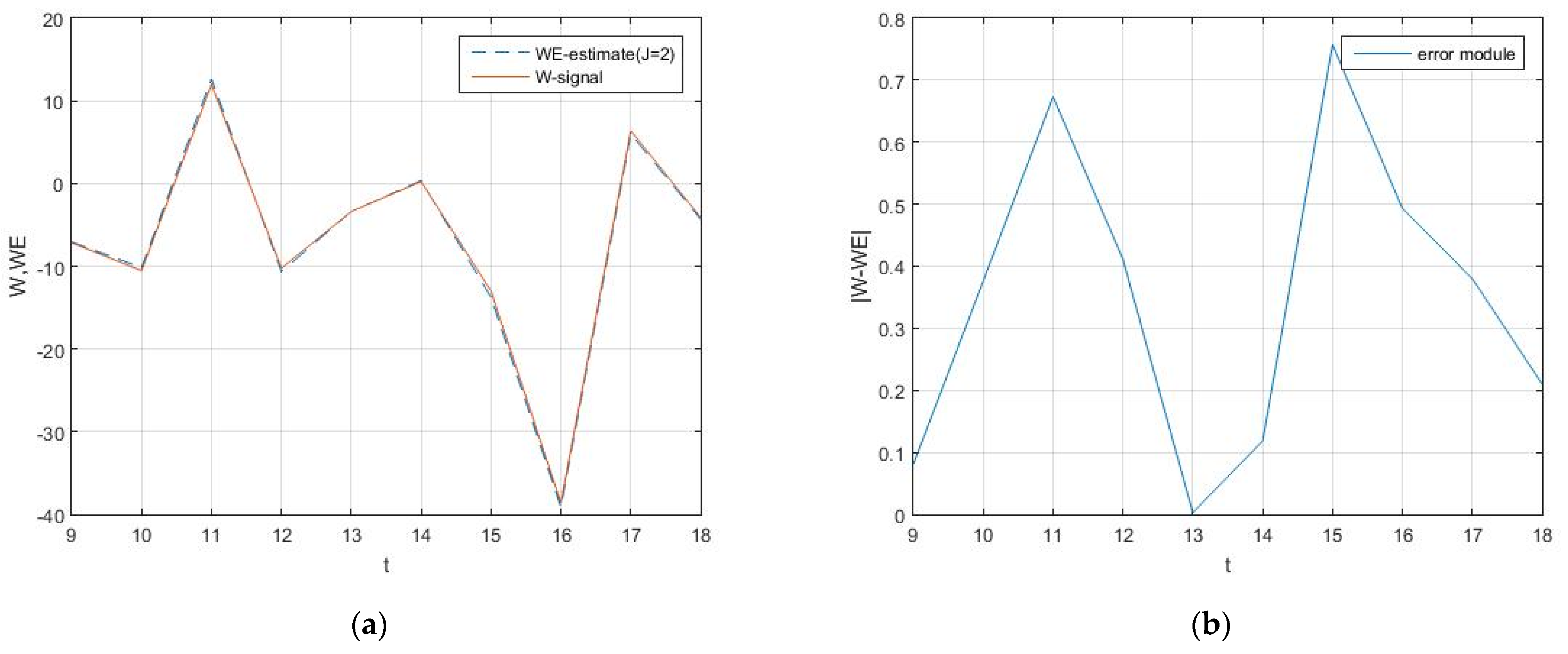
A typical realization method demonstrates high accuracy in Figure 1. As practice for quick calibration of typical devices we use, algorithms more simple than (82) were developed, computed and compared. This information is necessary for passport documentation.

The extrapolator takes values from −38.6099 to 11.9854. At the same time, the extrapolator error modulus does not exceed 0.7568 (Figure 1).

7. Conclusions

This article is devoted to problems with optimizing observable stochastic systems based on wavelet canonical expansions. Section 2 is devoted to different Bayes criteria in terms of risk theory. Following [1,2], in Section 3, basic formulae for optimal Bayes synthesis based on canonical expansions are given. Section 4 is dedicated to the solution of a general optimization problem using wavelet canonical expansions in case of complex nonstationary linear systems. In Section 5, a basic algorithm is given for the criterion of maximal probability that the signal will not exceed a particular value in absolute magnitude. An example of a radar-location extrapolator device is discussed.

The developed optimization methodology “quick probabilistic analytical numerical optimization” does not use statistical Monte Carlo methods.

Directions of future generalizations and implementations:

–

New models of scalar and vector OStS (nonlinear, with parametric noises, etc.):

–

New classes of the Bayes criteria.

The research was carried out using the infrastructure of the Shared Research Facilities “High Performance Computing and Big Data” (CKP “Informatics”) of FRC CSC RAS (Moscow).

References

1. Pugachev, V.S. Theory of Random Functions and Its Applications to Control Problems; Pergamon Press: Oxford, UK, 1965; 833p. [Google Scholar]
2. Pugachev, V.S.; Sinitsyn, I.N. Stochastic Systems Theory and Applications; World Scientific: Singapore, 2001. [Google Scholar]
3. Sinitsyn, I. Canonical Expansion of Random Functions and Its Application to Scientific Computer-Aided Support; Torus Press: Moscow, Russia, 2009. (In Russian) [Google Scholar]
4. Sinitsyn, I.N.; Sinitsyn, V.I.; Korepanov, E.R.; Belousov, V.V.; Sergeev, I.V. Development of Algorithmic Support for the Analysis of Stochastic Systems Based on Canonical Expansions of Random Functions. Autom. Remote Control 2011, 72, 405–415. [Google Scholar] [CrossRef]
5. Sinitsyn, I.N.; Sinitsyn, V.I.; Korepanov, E.R.; Konashenkova, T.D. Software Tools for Analysis and Synthesis of Stochastic Systems with High Availability (IV). Highly Available Syst. 2017, 13, 55–69. (In Russian) [Google Scholar]
6. Sinitsyn, I.N.; Sinitsyn, V.I.; Korepanov, E.R.; Konashenkova, T.D. Software Tools for Analysis and Synthesis of Stochastic Systems with High Availability (V). Highly Available Syst. 2018, 14, 59–70. (In Russian) [Google Scholar]
7. Sinitsyn, I.N.; Sinitsyn, V.I.; Korepanov, E.R.; Konashenkova, T.D. Software Tools for Analysis and Synthesis of Stochastic Systems with High Availability (VI). Highly Available Syst. 2018, 14, 40–56. (In Russian) [Google Scholar]
8. Sinitsyn, I.N.; Sinitsyn, V.I.; Korepanov, E.R.; Konashenkova, T.D. Software Tools for Analysis and Synthesis of Stochastic Systems with High Availability (VII). Highly Available Syst. 2019, 15, 47–61. (In Russian) [Google Scholar]
9. Arora, S.; Singh Brar, Y.; Kumar, S. Haar Wavelet Matrices for the Numerical Solutions of Differential Equations. Int. J. Comput. Appl. 2014, 97, 33–36. [Google Scholar] [CrossRef]
10. Stromberg, J.O. A modified Franklin system and higher-order spline systems on Rn as unconditional bases for Hardy spaces. In Proceedings of the Conference on Harmonic Analysis in Honor of Antoni Zygmund, Chicago, IL, USA, 23–28 March 1981; pp. 475–494. [Google Scholar]
11. Grossmann, A.; Morlet, J. Decomposition of Hardy Functions into Square Integrable Wavelets of Constant Shape. SIAM J. Math. Anal. 1984, 15, 723–736. [Google Scholar] [CrossRef]
12. Meyer, Y. Analysis at Urbana 1: Analysis in Function Spaces; Cambridge University Press: Cambridge, UK, 1989. [Google Scholar]
13. Mallat, S.G. Multiresolution approximations and wavelet orthonormal bases of L2 (R). Trans. Am. Math. Soc. 1989, 315, 69–87. [Google Scholar]
14. Daubechies, I. Orthonormal bases of compactly supported wavelets. Commun. Pure Appl. Math. 1988, 41, 909–996. [Google Scholar] [CrossRef] [Green Version]
15. Strang, G. Wavelets and dilation equations: A brief introduction. SIAM Rev. 1989, 31, 614–627. [Google Scholar] [CrossRef]
16. Hsiao, C.H. Haar wavelet approach to linear stiff systems. Math. Comput. Simul. 2004, 64, 561–567. [Google Scholar] [CrossRef]
17. Daubechies, I. Ten Lectures on Wavelets; SIAM: Philadelphia, PA, USA, 1992. [Google Scholar]
18. Chui, C.K. An Introduction to Wavelets; Academic Press: Boston, MA, USA, 1992. [Google Scholar]
19. Lepik, U. Numerical solution of differential equations using Haar wavelets. Math. Comput. Simul. 2005, 68, 127–143. [Google Scholar] [CrossRef]
20. Lepik, U. Numerical Solution of Evolution Equations by the Haar Wavelet Method. Appl. Math. Comput. 2007, 185, 695–704. [Google Scholar] [CrossRef]
21. Chen, C.F.; Hsiao, C.H. Haar Wavelet Method for Solving Lumped and Distributed Parameter Systems. IEE Proc. Control Theory Appl. 1987, 144, 87–94. [Google Scholar] [CrossRef] [Green Version]
22. Hsiao, C.H. State Analysis of Linear Time Delayed Systems via Haar Wavelets. Math. Comput. Simul. 1997, 44, 457–470. [Google Scholar] [CrossRef]
23. Cattani, C. Haar Wavelets Based Technique in Evolution Problems. Proc.-Est. Acad. Sci. Phys. Math. 2004, 1, 45–63. [Google Scholar] [CrossRef]
24. Hariharan, G. An Overview of Haar Wavelet Method for Solving Differential and Integral Equations. World Appl. Sci. J. 2013, 23, 1–14. [Google Scholar]
25. Hsiao, C.H.; Wu, S.P. Numerical Solution of Time-Varying Functional Differential Equations via Haar Wavelets. Appl. Math. Comput. 2007, 188, 1049–1058. [Google Scholar] [CrossRef]
26. Sinitsyn, I.; Sinitsyn, V.; Korepanov, E.; Konashenkova, T. Wavelet Modeling of Control Stochastic Systems at Complex Shock Disturbances. Mathematics 2021, 9, 2544. [Google Scholar] [CrossRef]
27. Sinitsyn, I.; Sinitsyn, V.; Korepanov, E.; Konashenkova, T. Optimization of Linear Stochastic Systems Based on Canonical Wavelet Expansions. Autom. Remote Control 2020, 81, 2046–2061. [Google Scholar] [CrossRef]
28. Sinitsyn, I.N.; Sinitsyn, V.I.; Korepanov, E.R.; Konashenkova, T.D. Software Tools for Analysis and Synthesis of Stochastic Systems with High Availability (XII). Highly Available Syst. 2021, 17, 26–44. (In Russian) [Google Scholar]
29. Sinitsyn, I.N.; Sinitsyn, V.I.; Korepanov, E.R.; Konashenkova, T.D. Software Tools for Analysis and Synthesis of Stochastic Systems with High Availability (XI). Highly Available Syst. 2021, 17, 25–40. (In Russian) [Google Scholar] [CrossRef]
30. Sinitsyn, I.N.; Sinitsyn, V.I.; Korepanov, E.R.; Konashenkova, T.D. Software Tools for Analysis and Synthesis of Stochastic Systems with High Availability (XIII). Highly Available Syst. 2021, 17, 16–35. (In Russian) [Google Scholar] [CrossRef]
31. Sinitsyn, I.N.; Sinitsyn, V.I.; Korepanov, E.R.; Konashenkova, T.D. Software Tools for Analysis and Synthesis of Stochastic Systems with High Availability (XV). Highly Available Syst. 2022, 18, 47–61. (In Russian) [Google Scholar] [CrossRef]
Figure 1. Graphs of: (a) signal extrapolation W and estimate extrapolation W * ; (b) module | W * W | .
Mathematics 10 01517 g001
Publisher’s Note: MDPI stays neutral with regard to jurisdictional claims in published maps and institutional affiliations.