Fully Connected Hashing Neural Networks for Indexing Large-Scale Remote Sensing Images

Abstract

With the emergence of big data, the efficiency of data querying and data storage has become a critical bottleneck in the remote sensing community. In this letter, we explore hash learning for the indexing of large-scale remote sensing images (RSIs) with a supervised pairwise neural network with the aim of improving RSI retrieval performance with a few binary bits. First, a fully connected hashing neural network (FCHNN) is proposed in order to map RSI features into binary (feature-to-binary) codes. Compared with pixel-to-binary frameworks, such as DPSH (deep pairwise-supervised hashing), FCHNN only contains three fully connected layers and incorporates another new constraint, so it can be significantly accelerated to obtain desirable performance. Second, five types of image features, including mid-level and deep features, were investigated in the learning of the FCHNN to achieve state-of-the-art performances. The mid-level features were based on Fisher encoding with affine-invariant local descriptors, and the deep features were extracted by pretrained or fine-tuned CNNs (e.g., CaffeNet and VGG-VD16). Experiments on five recently released large-scale RSI datasets (i.e., AID, NWPU45, PatternNet, RSI-CB128, and RSI-CB256) demonstrated the effectiveness of the proposed method in comparison with existing handcrafted or deep-based hashing methods.

1. Introduction

Nowadays, we are living in a period of big remote sensing data [1] because numerous Earth observation sensors provide a huge amount of remote sensing data for our lives; therefore, the development of fast and accurate content-based image retrieval (CBIR) methods is becoming increasingly important in the remote sensing community. In order to make better use of big data, machine learning methods are essential [2]. In 2007, Salakhutdinov and Hinton [3,4] proposed a hash learning method in the field of machine learning. Since then, the hashing method has been widely studied and applied in the fields of computer vision, information retrieval, pattern recognition, data mining, etc. [2]. Hash learning methods convert high-dimensional data into the form of binary codes through machine learning methods. At the same time, the transformed binary codes retain the neighboring relationships in the original high-dimensional space. In recent years, hash learning methods have rapidly developed into a research hotspot in the field of machine learning and big data.

Traditionally, the representation of remote sensing images (RSIs) is described by a real number vector with thousands of dimensions. Traditional remote sensing image retrieval methods usually describe images by using real vectors with thousands of dimensions. Each dimension can be stored in computer memory by floating-point data with four bytes, which may lead to the following issues: (1) The storage of a large-scale dataset requires many hard disks; (2) exhaustively searching for relevant images in a large-scale dataset is computationally expensive. When a 4096-dimensional feature of the fully connected layer in a deep network is expressed and stored, it takes 4096 × 4 bytes of storage space. Since one byte is equal to eight bits, the storage space of a 4096-dimensional real vector is 4096 × 4 × 8 bits. In contrast, when hash learning is used to map deep features, supposing that the deep features are mapped to 64 bits through hashing coding, the storage space used is eight bytes. In this case, in comparison with the storage space of 4096 × 4 × 8 bits, the hash learning method can greatly reduce the hard disk storage space of data and greatly improve the computational efficiency of image retrieval. To address the above issue, hashing-based approximate nearest neighbor search, which is a highly time-efficient search with a low storage space, is becoming a popular retrieval technique due to the emergence of big data. Hash mapping [5] represents an image as binary codes that contain a small number of bits, such as 32 bits (4 bytes), thereby significantly helping in the reduction of the amount of memory required for storage.

2. Related Work

Hashing-based retrieval methods can generally be divided into two categories: data-independent and data-dependent methods. As a popular data-independent method, random projection without training data is usually employed to generate hash functions, such as locality-sensitive hashing (LSH). Due to the limitation of data-independent hashing approaches [6], many recent methods based on an unsupervised or supervised manner were proposed in order to design more efficient hash functions. In the remote sensing community, there are only a few works on hash-based RSI retrieval. Demir and Bruzzone investigated two types of learning-based nonlinear hashing methods, namely, kernel-based unsupervised hashing (KULSH) and the kernel-based supervised LSH method (KSLSH). KULSH extended LSH to nonlinearly separable data by modeling each hash function as a nonlinear kernel hyperplane constructed from unlabeled data. KSLSH defined hash functions in the kernel space such that the Hamming distances from within-class images were minimized and those from between-class images were maximized. Both KULSH and KSLSH were used on bag-of-visual-words (BOVW) representations with SIFT descriptors [7]. Li and Ren [8,9] proposed partial randomness hashing (PRH) for RSI retrieval in two stages: (1) Random projections were generated to map image features (e.g., a 512-dimensional GIST descriptor) to a lower Hamming space in a data-independent manner; (2) a transformation weight matrix was used to learn based on training images. In KULSH, KSLSH, and PRH, the image representations (BOVW or GIST) were based on handcrafted feature extraction.

Benefiting from the rapid development of deep learning, Li et al. [10,11] investigated a deep hashing neural network (DHNN) and conducted comparisons of the binary quantization loss between the L1 and L2 norms. As an improved version of DPSH (deep pairwise-supervised hashing) [12], the DHNN improved the design of the sigmoid function and could perform feature learning and hash function learning simultaneously. Rather than designing handcrafted features, the DHNN could automatically learn different levels of feature abstraction, thereby resulting in a better description ability. However, the learning of the DHNN was time-consuming because deep feature learning and hash learning were performed in an end-to-end framework.

2.1. Convolutional Neural Network Hashing (CNNH)

CNNH combines the extraction of depth features and the learning of hash functions into a joint learning model [13,14]. Unlike the traditional method based on handcrafted features, CNNH is a supervised hash learning method, and it can automatically learn the appropriate feature representation and hash function from the pairwise labels by using the feature learning method of the neural network. CNNH is also the first deep hashing method to use paired label information as an input.

The CNNH method consists of two processes:

(1) 

Using the data samples to learn the hash function of the information.

Given n images, $\mathbf{X}=\left\{x_1,x_2,\cdots ,x_n\right\}$, and the similarity matrix S is defined as follows:

$$S_{ij}=\left\{\begin{array}{cc}+1& x_i,x_j\mathrm{are}\mathrm{similiar}\\ -1& x_i,x_j\mathrm{are}\mathrm{disimiliar}\end{array}\right.$$

(1)

The hash function that needs to be learned is defined as:

$$\mathrm{H}\left(X\right)=\left\{h_1\left(x\right),h_2\left(x\right),\cdots ,h_c\left(x\right)\right\}$$

(2)

where $\mathrm{H}\left(X\right)$ is an n by q binary matrix, and $h_k\left(x\right)\in {\left\{-1,1\right\}}^q$ is the k-th hash function in the matrix (the length of the function is q) and is also the hash code of the image $x_k$.

Supervised hashing uses the similarity matrix S and the data sample $\mathbf{X}$ to calculate a series of hash functions, that is, to decompose the similarity matrix S into $\mathrm{H}{\mathrm{H}}^T$ through gradient descent, where each row of H represents each the approximate hash codes corresponding to an image. The objective function of the above process is as follows:

$$\underset{H}{min}\sum _{i=1}^n\sum _{j=1}^n{\left(s_{ij}-\frac{1}{q}{H}_i{H}_j^T\right)}^2=\underset{H}{min}{∥\mathrm{S}-\frac{1}{q}{\mathrm{HH}}^T∥}_F^2$$

(3)

where ${∥·∥}_F$ is the Frobenius norm and $\mathrm{H}$ is the hash coding matrix.

(2) 

Learning the image feature representation and hash functions.

A convolutional network is used to learn the hash codes, and the learning process uses the cross-entropy loss function. The network has three convolutional layers, three pooling layers, one fully connected layer, and an output layer. The parameters of each layer are as follows: The numbers of filters of the first, second, and third convolutional layers are 32, 64, and 128 (with the size of 5 × 5); a dropout operation with a ratio of 0.5 is used in the fully connected layer.

After training the network, the image pixels can be used as inputs in order to obtain the image representation and hash codes. However, CNNH is not an end-to-end network.

2.2. Network-In-Network Hashing (NINH)

Rather than the paired labels used by the CNNH method, the NINH network uses triplets of images to train the model, which makes it an end-to-end deep hash learning method, and the layer is deeper than that of CNNH [15]. NINH integrates the feature representation and the learning of hash functions in a framework that allows them to promote each other and further improve performance.

Given the sample space of $\mathbf{X}$, we define the mapping function as $\mathrm{F}$:X$\to {\left\{0,1\right\}}^q$. The triplet information is $(\mathbf{X},{\mathbf{X}}_{+},{\mathbf{X}}_{-})$ and satisfies the following: The similarity between $\mathbf{X}$ and ${\mathbf{X}}_{+}$ is greater than that between $\mathbf{X}$ and ${\mathbf{X}}_{-}$. After mapping, the similarity between $F\left(\mathrm{X}\right)$ and $F\left({\mathrm{X}}_{+}\right)$ is greater than that between $F\left(\mathrm{X}\right)$ and $F\left({\mathrm{X}}_{-}\right)$.

The NINH method consists of three parts:

(1) 

The loss function.

The triplet-ranking hinge loss function is composed of three images, wherein the first image and the second image are similar, and the first image and the third image are dissimilar. The function is defined as:

$$\begin{array}{cc}\hfill & L_{\mathrm{trilet}}\left(F\left(X\right),F\left(X_{+}\right),F\left(X_{-}\right)\right)=\hfill \\ \hfill & max\left(0,1-\left({∥F\left(X\right)-F\left(X_{-}\right)∥}_H-{∥F\left(X\right)-F\left(X_{+}\right)∥}_H\right)\right)\hfill \end{array}$$

(4)

where $F\left(X\right),F\left(X_{+}\right),F\left(X_{-}\right)\in {\left\{0,1\right\}}^q$, ${∥·∥}_H$ represents the Hamming distance.

(2) 

The feature representation.

The CNN model is used to extract an effective feature representation from the input image. The CNN model that we used is an improved NIN (network-in-network) [16] network. The improvement of the network is the introduction of the convolution kernel, and the size of a convolutional layer is 1 × 1. In addition, an average pooled layer is used instead of the fully connected layer.

(3) 

The hash coding.

The feature-to-hash code mapping is performed by using the divide-and-encode module to reduce the redundancy between hash codes. At the same time, the sigmoid function is used to restrict the range of the output to [0,1], thereby avoiding discrete constraints.

2.3. Deep Pairwise-Supervised Hashing (DPSH)

DPSH based on pairs of images is used to compensate for the large workload of triplets [12,17]. Although the CNNH and DPSH methods are both based on pairs of information, the processes of feature learning and hash function learning are performed in two phases in the CNNH method. The two processes are independent of each other, and the DPSH method is an end-to-end deep learning framework that can perform feature learning and hash coding learning at the same time. The DPSH method mainly includes:

(1) 

Feature learning.

A convolutional neural network with a seven-layer structure is used for feature learning.

(2) 

Hash coding learning.

A discrete method is used to solve the NP-hard discrete optimization problem. For a set of binary hash codes $\mathrm{B}={\left\{b_i\right\}}_{i=1}^n$, the likelihood function L of the paired samples is defined as follows:

$$p\left(l_{i,j}\mid \mathrm{B}\right)=\left\{\begin{array}{ll}\mathrm{sigmoid}\left({\mathsf{\Psi }}_{i,j}\right)& l_{i,j}=1\\ 1-\mathrm{sigmoid}\left({\mathsf{\Psi }}_{i,j}\right)& l_{i,j}=0\end{array}\right.$$

(5)

where $\mathrm{sigmoid}\left({\mathsf{\Psi }}_{i,j}\right)=\frac{1}{1+e^{-{\psi }_{i,j}}}$, ${\psi }_{i,j}=\frac{b_i^T{b}_j}{p}$, and the value of p is 2. By taking the negative log-likelihood function $L[·]$ of the paired $l_{i,j}$, the following optimization problem can be obtained:

$$\underset{\mathbf{B}}{min}\zeta =-logp(L\mid \mathbf{B})=-\sum _{l_{i,j}\in L}logp\left(l_{i,j}\mid \mathbf{B}\right)-\sum _{l_{i,j}\in L}\left(l_{i,j}{\mathsf{\Psi }}_{i,j}-log\left(1+e^{-{\mathsf{\Psi }}_{i,j}}\right)\right)$$

(6)

Although existing methods cover handcrafted and CNN-based features, hash-based RSI retrieval still needs to be developed because the related works are scarce. For example, CNNH is an early representative model that combines deep convolutional networks with hash coding. It firstly decomposes the similarity matrix of samples in order to obtain the binary code of each sample, and then uses convolutional neural networks to fit the binary code. The fitting process is equivalent to a multi-label prediction problem. Although it has achieved significant performance improvements in comparison with traditional hand-designed-feature-based methods, it is still not an end-to-end method, and the image representation that is learned cannot be used, in turn, to update the binary code. Therefore, it still cannot fully exploit the powerful capabilities of deep models. To better tap into the potential of deep models, in this study, we propose a fully connected hashing neural network (FCHNN) to map the BOVW, pretrained, or fine-tuned deep features into binary codes with the aim of improving the RSI retrieval performance and learning efficiency. The main contributions are as follows: (1) An extended BOVW representation based on the affine-invariant local description and Fisher encoding is introduced, and this representation is competitive with deep features after hashing. (2) The FCHNN with three layers is proposed for pairwise-supervised hashing learning. The framework of the proposed feature-to-binary method has more advantages than that of a pixel-to-binary method (e.g., DPSH) in terms of the retrieval performance and efficiency. (3) In comparison with DSPH, another constraint is incorporated into the objective function of the FCHNN to accelerate the speed with which the desired results are obtained.

3. Proposed Method

The FCHNN consists of two parts: (1) feature extraction and (2) hashing learning based on a feature-to-binary framework, as shown in Figure 1. The proposed framework is beneficial for studying different types of features (either handcrafted or deep-based features). Based on the feature extraction, the FCHNN implements the hash coding of five types of features. These five types of features are Fisher vectors based on the affine-invariant local description, activation vector features extracted from the full connection layer based on pretrained and fine-tuning strategies, and activation vectors extracted using the CaffeNet and VGG-VD16 models, respectively. In order to be consistent, the Fisher vector also uses 4096-dimensional features. In the learning of the FCHNN, the same pair information as that used in DPSH is used for supervised learning, and the optimized learning process of the fully connected network is completed through random gradient descent.

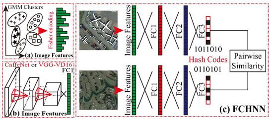
Figure 1. Framework of the proposed feature extraction and the FCHNN: (a,b) feature extraction stages; (c) the learning of the FCHNN.

A. 

$Feature$ $Extraction$

To give a comprehensive analysis of RSI representation and to investigate the generality of the FCHNN for different features, five types of feature extraction were employed.

Mid-Level Features: Mid-level representation consists of the detection of affine- invariant points of interest, extraction of SIFT descriptors, and Fisher encoding with GMM clustering. The interest-point detector selects a multi-scale Hessian implemented with the VLFeat toolbox [18], and a 128-dimensional SIFT descriptor is extracted for each point of interest. The SIFT descriptors are then transformed into RootSIFT [19] and 64-dimensional PCA-SIFT [20]. In the stage of Fisher encoding, a 4096-dimensional (2 × 32 × 64) Fisher vector can be obtained based on the PCA-SIFT and 32 GMM (Gaussian mixture model) clusters.

Deep Features: Two types of pretrained convolutional neural networks (CNNs), namely, CaffeNet and VGG-VD16, were employed to extract deep features. Both CNNs were implemented with MatConvNet [21] and trained on the ImageNet dataset. Both CaffeNet and VGG-VD16 included three fully connected layers. Given an input image and a CNN model, we extracted a 4096-dimensional activation vector from the antepenultimate fully connected layer as the deep features.

With the use of the fine-tuning strategy proposed by [22], the fine-tuned CaffeNet and VGG-VD16 could also be obtained by retraining the corresponding pretrained CNN on a training dataset until convergence. Given an input image and a fine-tuned CNN, 4096-dimensional activation vectors could also be obtained, similarly to the feature extraction using the pretrained CNN.

B. 

$FCHNN$

Architecture: As shown in Figure 1, the FCHNN consisted of three fully connected layers, with the aim of mapping the image features into a set of binary codes (0 or 1). The first two fully connected layers (denoted by FC1 and FC2) of the FCHNN contained 4096 neurons. Both FC1 and FC2 were followed by a nonlinear operation called rectified linear units (ReLU). The last fully connected layer (denoted as FC3) was the binary output containing N neural nodes. N corresponded to the desired number of bits after hashing. The architecture of the FCHNN was similar to that of the last three fully connected layers of AlexNet, except for the number of output nodes. The FCHNN has the following characteristics: (1) It is a feature-to-binary rather than pixel-to-binary framework; (2) it is general for both handcrafted and deep features; (3) the use of fewer layers can significantly improve its learning speed.

Object Function: Given n training images, $\mathbf{Z}={\left\{z_i\right\}}_{i=1}^n$, where $z_i$ is a vector (image features shown in Figure 1) of the ith image. A set of pairwise labels $\mathbf{L}=\left\{l_{i,j}\right\}$ that satisfy $l_{i,j}\in \left\{0,1\right\}$ is constructed to provide the supervised information. $l_{i,j}=1$ indicates that $z_i$ and $z_j$ are similar (within-class samples); otherwise ($l_{i,j}=0$), $z_i$ and $z_j$ are dissimilar (between-class samples). The FCHNN aims to map $z_i$ to binary codes $b_i\in {\left\{-1,1\right\}}^d$ with d bits, causing $b_i$ and $b_j$ to have a low Hamming distance if $l_{i,j}=1$ or a high Hamming distance if $l_{i,j}=0$.

Here, we adopt the same definition as that in Equation (5). Inspired by deep hashing neural networks (DHNNs), we parameterize Equation (5) as $p=sd$, where s is the similarity factor and d is the length of the hash codes. This operation can not only enhance the flexibility of the algorithm, but can also enable the algorithm to have optimal performance when facing hash codes of different lengths. To solve the optimization problem of Equation (6), its discrete form can be rewritten as follows:

$$\begin{array}{cc}\hfill \underset{\mathbf{B},\mathbf{A}}{min}\zeta & =-\sum _{l_{i,j}\in \mathbf{L}}\left(l_{i,j}{\mathsf{\Lambda }}_{i,j}-log\left(1+e^{{\mathsf{\Lambda }}_{i,j}}\right)\right)\hfill \\ \hfill \mathrm{s}.\mathrm{t}.& a_i=b_i\forall i=1,2,\cdots ,n\hfill \\ \hfill a_i& \in {\mathbb{R}}^{c\times 1}\forall i=1,2,\cdots ,n\hfill \\ \hfill b_i& \in {\{-1,1\}}^c\forall i=1,2,\cdots ,n\hfill \end{array}$$

(7)

where ${\mathsf{\Lambda }}_{i,j}=\frac{a_i^T{a}_j}{sd}$ and $\mathrm{A}={\left\{a_i\right\}}_{i=1}^n$.

By taking the negative log-likelihood of the pairwise labels $l_{i,j}$ in $\mathbf{L}$, the following objective function can be formed:

$$\underset{\mathbf{B},\mathbf{A}}{min}\zeta =-\sum _{l_{i,j}\in \mathbf{L}}\left(l_{i,j}{\mathsf{\Lambda }}_{i,j}-log\left(1+e^{{\mathsf{\Lambda }}_{i,j}}\right)\right)+\alpha \sum _{i=1}^n{∥b_i-a_i∥}_2^2$$

(8)

where $\mathrm{A}={\left\{a_i\right\}}_{i=1}^n$; $a_i={\mathbf{W}}^{T}f(z_i;\theta )+v$, and $\theta$ denotes the FC1 and FC2 parameters of the FCHNN; $f(z_i;\theta )$ denotes the FC2 output, $\mathbf{W}\in {\mathbb{R}}^{4096\times d}$ denotes a weighted matrix containing the fully connected weights between FC2 and FC3, $v\in {\mathbb{R}}^{c\times 1}$ is a bias vector, and $\alpha$ is a hyper-parameter.

Equation (8) aims to make the FCHNN’s output and the final binary code $b_i$ as similar as possible. In addition, we introduce another constraint into the objective function, and Equation (8) can be rewritten as follows:

$$\underset{\mathbf{B},\mathbf{A}}{min}\zeta =-\sum _{l_{i,j}\in \mathbf{L}}\left(l_{i,j}{\mathsf{\Lambda }}_{i,j}-log\left(1+e^{{\mathsf{\Lambda }}_{i,j}}\right)\right)+\alpha \sum _{i=1}^n{∥b_i-a_i∥}_2^2+\beta \sum _{l_{i,j}\in \mathbf{L}}\left({\mathsf{\Psi }}_{i,j}-l_{i,j}\right)b_i^T{a}_i$$

(9)

where $b_i^T{a}_i$ should be as large as possible, while ${\mathsf{\Psi }}_{i,j}-l_{i,j}$ should be as small as possible. The third term, which can significantly accelerate the learning speed in order to obtain desirable results, considers the performance of the final hash codes. Thus, we can obtain:

$$\begin{array}{c}\underset{\mathbf{B},\mathbf{W},v,\theta }{\min }\zeta =-{\displaystyle \sum _{l_{i,j}\in \mathbf{L}}}\left(l_{i,j}{\mathsf{\Lambda }}_{i,j}-\log \left(1+e^{{\mathsf{\Lambda }}_{i,j}}\right)\right)+\\ \mathrm{alpha}{\displaystyle \sum _{i=1}^n}{∥b_i-{\mathbf{W}}^{T}f\left(z_i;\theta \right)+v∥}_2^2+\beta {\displaystyle \sum _{l_{i,j}\in \mathbf{L}}}\left({\mathsf{\Psi }}_{i,j}-l_{i,j}\right)b_i^T\left({\mathbf{W}}^{T}f\left(z_i;\theta \right)+v\right)\end{array}$$

(10)

where $\mathbf{B},\mathbf{W},v$ and $\theta$ are the parameters that need to to be learned.

Learning: The learning of the FCHNN is summarized in Algorithm 1. In each iteration, a mini-batch of training images is collected from the entire training set in order to alternately update the parameters. In particular, $b_i$ can be directly optimized by $b_i=sign\left(a_i\right)=sign({\mathbf{W}}^{T}f\left(z_{i;\theta }\right)+v)$. For $\mathbf{W},v$ and $\theta$, we first compute the derivatives of the objective function for $a_i$:

$$\frac{\partial \zeta }{\partial a_i}=\sum _{j=1}^n\left({\mathsf{\Lambda }}_{i,j}-l_{i,j}\right)a_j+2\alpha \left(a_i-b_i\right)+\beta \sum _{j=1}^n\left({\mathsf{\Psi }}_{i,j}-l_{i,j}\right)b_j$$

(11)

Then, $\mathbf{W},v$ and $\theta$ can be updated through back-propagation, as in [23,24].

Algorithm 1: Learning for the FCHNN

Input: Training samples $\mathbf{Z}={\left\{{\mathbf{z}}_i\right\}}_{i=1}^n$ and pairwise labels $\mathbf{L}=\left\{{\mathbf{l}}_{i,j}\right\}$

Output: $\mathbf{B}$, $\mathbf{W}$, $\mathbf{v}$, and $\theta$

FCHNN initialization: All fully connected weights are randomly initialized by a Gaussian distribution with a mean of 0 and variance of 0.01.

Repeat: Sampling a minibatch of samples randomly from $\mathbf{Z}$, each sample ${\mathbf{Z}}_i$ in the minibatch performs: (1) Calculation of $f\left({\mathbf{Z}}_i;\theta \right)$ by using forward propagation (2) Computation of ${\mathbf{a}}_i={\mathbf{W}}^{T}f\left({\mathbf{z}}_i;\theta \right)+\mathbf{v}$ (3) Computation of the binary code of ${\mathbf{Z}}_i$ by using ${\mathbf{b}}_i=\mathrm{sign}\left({\mathbf{a}}_i\right)$ (4) Computation of derivatives for ${\mathbf{Z}}_i$ (5) Update of $\mathbf{W}$, $\mathbf{v}$, and $\theta$ via back-propagation Until a fixed number of iterations is reachd

Output of the FCHNN: The model obtained after the network learning of the FCHNN can be applied to the mapping of image features other than those in the training set. For any given input image, first, we can extract the corresponding image features as the input of the FCHNN, extract the output of the FCHNN through forward propagation, and do the following:

$$b_i=\mathrm{sign}\left({\mathbf{W}}^{T}f\left(z_i;\theta \right)+v\right)$$

(12)

where $b_i$ represents the final hash codes.

4. Experiments and Discussion

Extensive experiments were conducted on five recently released large-scale datasets, namely, AID [25], NWPU [26], PatternNet [27], RSI-CB128 [28], and RSI-CB256 [28], as shown in Figure 2. AID contains 30 RSI scene classes collected from multi-source-based Google Earth imagery, including 10,000 RGB images with 600 × 600 pixels. Each class consists of different numbers of images, ranging from 220 to 420; the spatial resolution of this dataset ranges from 0.5 to 8 m. NWPU contains 45 RSI scene classes collected from Google Earth, including 31,500 RGB images with 256 × 256 pixels. Each class contains 700 images, and the spatial resolution of this dataset ranges from 0.2 to 30 m in most cases. PatternNet contains 38 RSI classes collected from Google Earth imagery or the Google Maps API, including 30,400 RGB images with 256 × 256 pixels. Each class contains 800 images, and the spatial resolution of this dataset ranges from 0.062 to 4.693. RSI-CB is composed of RSI-CB128 and RSI-CB256, which are two large-scale RSI datasets collected from Google Earth and Bing Maps. RSI-CB128 contains 45 RSI scene classes, including more than 36,000 RGB images with 128 × 128 pixels. RSI-CB256 contains 35 RSI scene classes, including more than 24,000 RGB images with 256 × 256 pixels. The resolution of RSI-CB (both RSI-CB128 and RSI-CB256) ranges from 0.22 to 3 m.

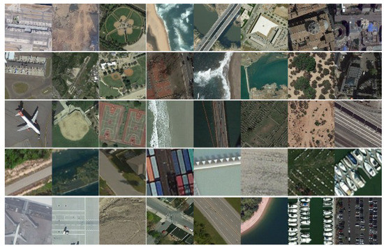
Figure 2. Datasets. From top to bottom: AID, NWPU, PatternNet, RSI-CB128, and RSI-CB256.

A. 

Experimental setup and evaluation strategy

Each dataset was randomly divided into five parts—four parts for training and one for testing. Given a dataset, the fine-tuning process of CaffeNet or VGG-VD16 was performed on the training set with a workstation with a 3.4 GHz Intel CPU and 32 GB of memory, and an NVIDIA Quadro K2200 GPU was used for acceleration. The fine-tuning parameters, such as the learning rate, batchSize, weightDecay, and momentum, were set to 0.001, 256, 0.0005, and 0.9, respectively.

For the FCHNN, we used a validation set to choose the hyper-parameters $s,\alpha ,$ and $\beta$, and we found that good performance could be achieved by setting $s=2,\alpha =50$, and $\beta =1$, which were then used for all dataset experiments with $d=16,d=32,$ and $d=64$, where $s=2$ was the similarity factor. After the feature vectors were normalized, they needed to be dot-multiplied by 500. In the experiment, to better adapt the Fisher vector to the FCHNN, we found that scaling up the Fisher vector by a certain ratio could improve the accuracy of hash retrieval. Thus, 500 was the empirical value that we obtained after a series of comparative analyses. Of course, if we did not scale up the Fisher vector, we could also obtain a considerable retrieval effect.

To evaluate the retrieval performance, each image (represented by binary codes) in the testing dataset was used as a query to sequentially compute the Hamming distance between the query and training images in order to obtain the ranking results, which were then used to compute the average precision. The final mean average precision (mAP) [18,29,30] was the averaged result over all queries. Precision–recall curves were also used to plot the tradeoff between precision (Precision = TP/(TP + FP)) and recall (Recall = TP/(TP + FN)), where TP is a true positive, FP is a false positive, and FN is a false negative.

B. 

Evaluation of the retrieval performance

Given a training dataset with multiple classes, the optimization of the FCHNN was based on supervised learning with back-propagation (BP) by computing the derivatives of a defined objective function. The supervised information could be obtained with pairs of images (similar or dissimilar) from the training dataset; meanwhile, the objective function was based on pairwise images (labels).

Unlike DPSH and DHNNs, the FCHNN has a small-sized network architecture and learns the linear–nonlinear transformation with multiple layers for mid-level or deep features, rather than the original image. There are two differences between DPSH [31] and the proposed FCHNN in terms of optimization: (1) Firstly, the weighted sigmoid function is selected to allow the FCHNN to have better performance; (2) secondly, the FCHNN introduces another constraint term in order to improve the convergence of the network learning.

Table 1 and Figure 3 show comparisons of the hash retrieval performance (mAP) on five datasets, on which four methods were compared; these were PRH [8], KULSH [32], KSLSH [32], and DPSH [24,31]. PRH is a method of learning hash functions by using a locally random strategy. Firstly, images are mapped to Hamming space in a data-independent manner by using a random projection algorithm. Secondly, learning transforms the weight matrix from the training data of remote sensing images in a more efficient way. However, this method only extracts GIST features; it is a hash coding method based on handcrafted features. For a comprehensive comparative analysis, we further combined PRH with BOW and Fisher vector coding in order to extract mid-level features and use them for hash coding. KULSH [32,33,34] is based on the LSH method, and it is for achieving fast processing of kernel data with arbitrary kernel functions. KULSH [35] only exploits the BOVW method. Similarly, in order to ensure the comprehensiveness of our comparative research, we also combined the KULSH method with the GIST features and the Fisher vector coding method as the middle-layer expression, and then with hash coding. KSLSH [32,36] is a limited supervised method that uses similar and dissimilar pairwise information, achieves high-quality hash function learning based on sufficient training datasets, and, finally, maps data to Hamming space. The distance within similar data is the smallest, and the distance within dissimilar data is the largest in the Hamming space.

Table 1. Comparison of the hash retrieval performance (mAP) on the AID, NWPU45, PatternNet, RSI-CB128, and RSI-CB256 datasets.

Methods	Coding Length (Bit)	AID	NWPU45	PatternNet	RSI-CB128	RSI-CB256
PRH (GIST) [8]	16	0.0712	0.0405	0.0872	0.0754	0.0836
	32	0.0541	0.0349	0.0968	0.0831	0.0978
	64	0.0559	0.0376	0.1304	0.0957	0.1072
PRH (BOVW) [8]	16	0.1052	0.0737	0.1746	0.1363	0.1677
	32	0.1244	0.0863	0.2604	0.1893	0.2158
	64	0.1561	0.1041	0.3077	0.2502	0.2969
PRH (FV-AI) [8]	16	0.1558	0.0955	0.3253	0.1957	0.2636
	32	0.1894	0.1310	0.4244	0.2631	0.3468
	64	0.2357	0.157	0.5336	0.3149	0.4525
KULSH (GIST) [32]	16	0.0413	0.0241	0.0304	0.0293	0.0402
	32	0.0370	0.0232	0.0343	0.0289	0.0439
	64	0.0384	0.0233	0.0299	0.0313	0.0367
KULSH (BOVW) [32]	16	0.0410	0.0267	0.0431	0.0311	0.0373
	32	0.0378	0.0257	0.0329	0.0366	0.0447
	64	0.0394	0.0252	0.0356	0.0366	0.0447
KULSH (FV-AI) [32]	16	0.0933	0.0296	0.1323	0.0347	0.0410
	32	0.1458	0.0270	0.1874	0.0429	0.0457
	64	0.1983	0.0319	0.3366	0.0366	0.0539
KSLSH (GIST) [32]	16	0.1804	0.0744	0.3391	0.2573	0.3711
	32	0.2118	0.0816	0.4037	0.2885	0.4113
	64	0.2387	0.0904	0.4356	0.3122	0.4627
KSLSH (BOVW) [32]	16	0.2993	0.1734	0.5154	0.4342	0.4592
	32	0.3354	0.2527	0.6208	0.5163	0.5499
	64	0.3691	0.2861	0.6950	0.5546	0.5849
KSLSH (FV-AI) [32]	16	0.5343	0.3432	0.8351	0.6085	0.7372
	32	0.6115	0.4209	0.8851	0.6732	0.7936
	64	0.6531	0.4724	0.9281	0.7142	0.8279
DPSH [17]	16	0.6183	0.3656	0.5589	0.6061	0.7015
	32	0.8805	0.6066	0.8866	0.8106	0.8701
	64	0.9246	0.7481	0.9940	0.8438	0.9104
FCHNN (FV-AI)	16	0.6894	0.5713	0.7281	0.6066	0.7036
	32	0.9127	0.7320	0.9248	0.8961	0.9775
	64	0.9154	0.9035	0.9934	0.9593	0.9902
FCHNN (P-CaffeNet)	16	0.6733	0.6235	0.7299	0.6514	0.7272
	32	0.9181	0.7223	0.9077	0.9007	0.9769
	64	0.9300	0.8749	0.9901	0.9668	0.9918
FCHNN (F-CaffeNet)	16	0.7328	0.6793	0.8461	0.6812	0.7691
	32	0.9386	0.7463	0.9471	0.9141	0.9827
	64	0.9432	0.9131	0.9938	0.9782	0.9930
FCHNN (P-VGG-VD16)	16	0.6845	0.5905	0.7491	0.6551	0.7313
	32	0.9245	0.7366	0.8893	0.9016	0.9823
	64	0.9374	0.8890	0.9925	0.9756	0.9864
FCHNN (F-VGG-VD16)	16	0.7825	0.7417	0.9264	0.7023	0.7666
	32	0.9568	0.8582	0.9689	0.9177	0.9820
	64	0.9583	0.9509	0.9963	0.9845	0.9950

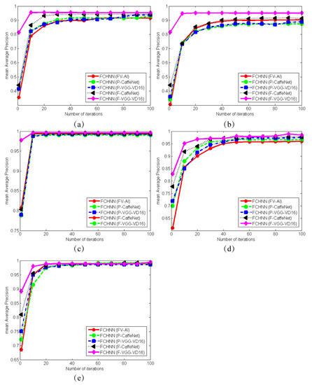
Figure 3. Comparison of five types of features in RSI retrieval based on five datasets. All results are given as the mean average precision (mAP). (a) AID dataset, (b) NWPU45 dataset, (c) PatternNet dataset, (d) RSI-CB128 dataset, and (e) RSI-CB256 dataset.

In general, the PRH, KULSH, and KSLSH methods are hash coding methods that use handcrafted features. Deep pairwise-supervised hashing (DPSH) is a deep hashing method that implements both feature learning and hash coding learning in a complete framework, and it uses pairwise image information. The FCHNN is our proposed method.

As we can see in Table 1 and Figure 3, the deep hash method had obvious performance advantages over the handcrafted-feature-based methods; compared with the DPSH method, the proposed FCHNN method obtained a higher retrieval accuracy, and the FCHNN had good generality, making it suitable for the hashing of both artificial design features and depth features. Among the five types of features, the features extracted from the fine-tuned VGG-VD16 model achieved the highest accuracy, which was better than that of the features extracted from the pre-trained VGG-VD16 model. So, it was verified that the fine-tuning strategy could effectively improve the retrieval results.

C. 

The effect of the number of iterations in the process of network learning

We compared the image retrieval accuracy (mAP) of five types of features for remote sensing image retrieval tasks on five large-scale datasets, and the mAP value was based on the result of 64-bit hash coding. We obtained the following conclusions: (1) The experiments on the five datasets showed that the proposed FCHNN method was able to obtain relatively stable precision in 40 iterations; (2) the features extracted by the fine-tuned VGG-VD16 model had the highest retrieval accuracy among the five types of features; the accuracy of the two fine-tuned CNN models was generally higher than that of the pre-trained model, which further validated the effectiveness of the fine-tuning strategy; (3) as the number of FCHNN iterations increased, the accuracy was improved.

D. 

The effect of the training size

Because Table 1 showed that features extracted from the fine-tuned VGG-VD16 model (i.e., F-VGG-VD16) were able to achieve the highest accuracy, we also employed the F-VGG-VD16 model to perform experiments on the five datasets in order to study the impacts of different training sizes on the training accuracy, as shown in Table 2. Clearly, as the training size increased, the performance of the model also gradually increased. This is consistent with the general knowledge in deep learning, which holds that larger datasets can lead to better performance of a model.

Table 2. Effects of the training size on the model performance.

Training Size ${}^1$	Dataset
	AID	NWPU45	PatternNet	RSI-CB128	RSI-CB256
20%	0.3723	0.3197	0.4503	0.3927	0.4103
40%	0.5564	0.5321	0.6057	0.5881	0.6117
60%	0.7927	0.7769	0.8122	0.8233	0.7975
80%	0.9583	0.9509	0.9963	0.9845	0.9950

¹ Training size: the percentage of the number of training samples with respect to the total number of samples.

E. 

Comparison with other methods

As shown in Figure 4, we compared the PR curves of the FCHNN and DPSH methods for the five datasets. The red curve represents the DPSH method and the green curve represents the FCHNN method. The input of the FCHNN was the best of the five features, that is, features extracted from the fine-tuned VGG-VD16 model (F-VGG-VD16). The results of the two methods used for the comparison were based on 64-bit hash coding. The experiments on the five datasets showed that the FCHNN was able to obtain better retrieval accuracy than that of DPSH.

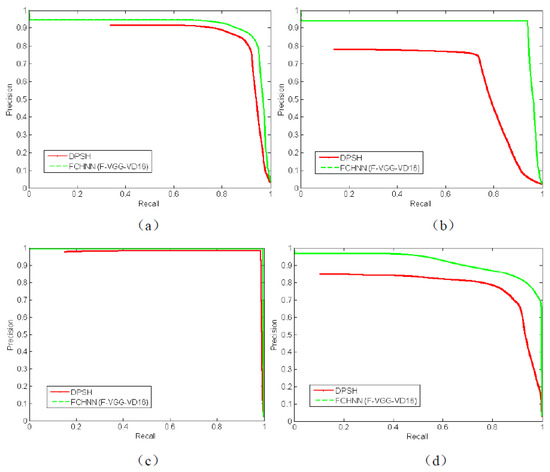
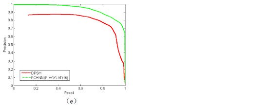
Figure 4. PR comparisons between the FCHNN and DPSH. (a) AID, (b) NWPU45, (c) PatternNet, (d) RSI-CB128, and (e) RSI-CB256.

5. Conclusions

We proposed a hash neural network model called the FCHNN that has three layers of fully connected layers in order to achieve efficient storage and retrieval of remote sensing images. The first two layers of the network contain 4096 neurons, and the last layer of the network contains N neurons. Through the supervised learning of pairwise images, hash coding mapping of different types of features, including mid-level representations based on low-level feature extraction, pre-trained deep features, and fine-tuned depth features, can be realized, and bit–bit binary can be achieved. The FCHNN is a network of features transmitted into binary code. In comparison with end-to-end networks of pixel-to-binary frameworks, the FCHNN has a higher learning efficiency and retrieval precision. Experiments on five large-scale remote sensing image datasets showed that the FCHNN has good versatility in the hash mapping of different types of features. The deep features extracted from the fine-tuned VGG-VD16 model achieved the best retrieval performance when used as input for the FCHNN.

In the face of massive amounts of remote sensing data, data storage and retrieval based on high-level features have a low efficiency and high computational complexity. In comparison with CNNH, DPSH, and other models, our proposed model (FCHNN) has great advantages. On the one hand, the FCHNN only contains three layers of fully connected layers, and it uses the supervised information of pairwise labels to learn the hash function. In comparison with the end-to-end deep hash learning method based on label pairs, its learning speed is faster; on the other hand, the FCHNN is a network based on feature-to-binary encoding, and it can obtain a higher retrieval precision. In addition, the FCHNN can not only learn artificially designed features, such as the Fisher vector encoding, but can also learn deep features, which have good universality. Importantly, in consideration of storage space, when mapping 4096-dimensional features to 64 bits, the FCHNN requires only eight bytes. Therefore, our model has good application prospects in the storage and retrieval of remote sensing images.

References

- Heppenstall, A.; Crooks, A.; Malleson, N.; Manley, E.; Ge, J.; Batty, M. Future developments in geographical agent-based models: Challenges and opportunities. Geogr. Anal. 2021, 53, 76–91. [Google Scholar] [CrossRef]
- Singh, A.; Gupta, S. Learning to hash: A comprehensive survey of deep learning-based hashing methods. Knowl. Inf. Syst. 2022, 64, 2565–2597. [Google Scholar] [CrossRef]
- Yao, T.; Wang, G.; Yan, L.; Kong, X.; Su, Q.; Zhang, C.; Tian, Q. Online latent semantic hashing for cross-media retrieval. Pattern Recognit. 2019, 89, 1–11. [Google Scholar] [CrossRef]
- Song, G.; Tan, X.; Zhao, J.; Yang, M. Deep robust multilevel semantic hashing for multi-label cross-modal retrieval. Pattern Recognit. 2021, 120, 108084. [Google Scholar] [CrossRef]
- Li, Y.; Ma, J.; Zhang, Y. Image retrieval from remote sensing big data: A survey. Inf. Fusion 2021, 67, 94–115. [Google Scholar] [CrossRef]
- Gu, Y.; Wang, Y.; Li, Y. A survey on deep learning-driven remote sensing image scene understanding: Scene classification, scene retrieval and scene-guided object detection. Appl. Sci. 2019, 9, 2110. [Google Scholar] [CrossRef]
- Bansal, M.; Kumar, M.; Kumar, M. 2D object recognition: A comparative analysis of SIFT, SURF and ORB feature descriptors. Multimed. Tools Appl. 2021, 80, 18839–18857. [Google Scholar] [CrossRef]
- Li, P.; Ren, P. Partial randomness hashing for large-scale remote sensing image retrieval. IEEE Geosci. Remote Sens. Lett. 2017, 14, 464–468. [Google Scholar] [CrossRef]
- Tan, X.; Zou, Y.; Guo, Z.; Zhou, K.; Yuan, Q. Deep Contrastive Self-Supervised Hashing for Remote Sensing Image Retrieval. Remote Sens. 2022, 14, 3643. [Google Scholar] [CrossRef]
- Li, Y.; Zhang, Y.; Huang, X.; Zhu, H.; Ma, J. Large-scale remote sensing image retrieval by deep hashing neural networks. IEEE Trans. Geosci. Remote Sens. 2017, 56, 950–965. [Google Scholar] [CrossRef]
- Shan, X.; Liu, P.; Wang, Y.; Zhou, Q.; Wang, Z. Deep hashing using proxy loss on remote sensing image retrieval. Remote Sens. 2021, 13, 2924. [Google Scholar] [CrossRef]
- Zhao, Q.; Xu, Y.; Wei, Z.; Han, Y. Non-intrusive load monitoring based on deep pairwise-supervised hashing to detect unidentified appliances. Processes 2021, 9, 505. [Google Scholar] [CrossRef]
- Zhang, Q.Y.; Li, Y.Z.; Hu, Y.J. A retrieval algorithm for encrypted speech based on convolutional neural network and deep hashing. Multimed. Tools Appl. 2021, 80, 1201–1221. [Google Scholar] [CrossRef]
- Li, T.; Zhang, Z.; Pei, L.; Gan, Y. HashFormer: Vision Transformer Based Deep Hashing for Image Retrieval. IEEE Signal Process. Lett. 2022, 29, 827–831. [Google Scholar] [CrossRef]
- Lai, H.; Pan, Y.; Liu, Y.; Yan, S. Simultaneous feature learning and hash coding with deep neural networks. In Proceedings of the IEEE Conference on Computer Vision and Pattern Recognition, Boston, MA, USA, 7–12 June 2015; pp. 3270–3278. [Google Scholar]
- Lin, M.; Chen, Q.; Yan, S. Network in network. arXiv 2013, arXiv:1312.4400. [Google Scholar]
- Li, W.J.; Wang, S.; Kang, W.C. Feature Learning Based Deep Supervised Hashing with Pairwise Labels. In Proceedings of the Twenty-Fifth International Joint Conference on Artificial Intelligence, IJCAI’16, New York, NY, USA, 9–15 July 2016; pp. 1711–1717. [Google Scholar]
- Vedaldi, A.; Fulkerson, B. VLFeat: An open and portable library of computer vision algorithms. In Proceedings of the 18th ACM International Conference on Multimedia, Firenze, Italy, 25–29 October 2010; pp. 1469–1472. [Google Scholar]
- Vijayan, V.; Pushpalatha, K. A comparative analysis of RootSIFT and SIFT methods for drowsy features extraction. Procedia Comput. Sci. 2020, 171, 436–445. [Google Scholar] [CrossRef]
- Dai-Hong, J.; Lei, D.; Dan, L.; San-You, Z. Moving-object tracking algorithm based on PCA-SIFT and optimization for underground coal mines. IEEE Access 2019, 7, 35556–35563. [Google Scholar] [CrossRef]
- Vedaldi, A.; Lenc, K. Matconvnet: Convolutional neural networks for matlab. In Proceedings of the 23rd ACM International Conference on Multimedia, Brisbane, Australia, 26–30 October 2015; pp. 689–692. [Google Scholar]
- Nogueira, K.; Penatti, O.A.; dos Santos, J.A. Towards better exploiting convolutional neural networks for remote sensing scene classification. Pattern Recognit. 2017, 61, 539–556. [Google Scholar] [CrossRef]
- Gu, G.; Liu, J.; Li, Z.; Huo, W.; Zhao, Y. Joint learning based deep supervised hashing for large-scale image retrieval. Neurocomputing 2020, 385, 348–357. [Google Scholar] [CrossRef]
- Chen, Y.; Lu, X. Deep discrete hashing with pairwise correlation learning. Neurocomputing 2020, 385, 111–121. [Google Scholar] [CrossRef]
- Xia, G.S.; Hu, J.; Hu, F.; Shi, B.; Bai, X.; Zhong, Y.; Zhang, L.; Lu, X. AID: A benchmark data set for performance evaluation of aerial scene classification. IEEE Trans. Geosci. Remote Sens. 2017, 55, 3965–3981. [Google Scholar] [CrossRef]
- Cheng, G.; Han, J.; Lu, X. Remote sensing image scene classification: Benchmark and state of the art. Proc. IEEE 2017, 105, 1865–1883. [Google Scholar] [CrossRef]
- Zhou, W.; Newsam, S.; Li, C.; Shao, Z. PatternNet: A benchmark dataset for performance evaluation of remote sensing image retrieval. ISPRS J. Photogramm. Remote Sens. 2018, 145, 197–209. [Google Scholar] [CrossRef]
- Li, H.; Tao, C.; Wu, Z.; Chen, J.; Gong, J.; Deng, M. Rsi-cb: A large scale remote sensing image classification benchmark via crowdsource data. arXiv 2017, arXiv:1705.10450. [Google Scholar]
- Zhou, W.; Newsam, S.; Li, C.; Shao, Z. Learning low dimensional convolutional neural networks for high-resolution remote sensing image retrieval. Remote Sens. 2017, 9, 489. [Google Scholar] [CrossRef]
- Zhuo, Z.; Zhou, Z. Low dimensional discriminative representation of fully connected layer features using extended largevis method for high-resolution remote sensing image retrieval. Sensors 2020, 20, 4718. [Google Scholar] [CrossRef]
- Zhang, X.; Zhou, L.; Bai, X.; Luan, X.; Luo, J.; Hancock, E.R. Deep supervised hashing using symmetric relative entropy. Pattern Recognit. Lett. 2019, 125, 677–683. [Google Scholar] [CrossRef]
- Demir, B.; Bruzzone, L. Hashing-based scalable remote sensing image search and retrieval in large archives. IEEE Trans. Geosci. Remote Sens. 2015, 54, 892–904. [Google Scholar] [CrossRef]
- Jafari, O.; Maurya, P.; Nagarkar, P.; Islam, K.M.; Crushev, C. A survey on locality sensitive hashing algorithms and their applications. arXiv 2021, arXiv:2102.08942. [Google Scholar]
- Zhou, W.; Liu, H.; Lou, J.; Chen, X. Locality sensitive hashing with bit selection. Appl. Intell. 2022, 52, 14724–14738. [Google Scholar] [CrossRef]
- Shan, X.; Liu, P.; Gou, G.; Zhou, Q.; Wang, Z. Deep hash remote sensing image retrieval with hard probability sampling. Remote Sens. 2020, 12, 2789. [Google Scholar] [CrossRef]
- Roy, S.; Sangineto, E.; Demir, B.; Sebe, N. Metric-learning-based deep hashing network for content-based retrieval of remote sensing images. IEEE Geosci. Remote Sens. Lett. 2020, 18, 226–230. [Google Scholar] [CrossRef]
Publisher’s Note: MDPI stays neutral with regard to jurisdictional claims in published maps and institutional affiliations. |
© 2022 by the authors. Licensee MDPI, Basel, Switzerland. This article is an open access article distributed under the terms and conditions of the Creative Commons Attribution (CC BY) license (https://creativecommons.org/licenses/by/4.0/).