Design of a Compliant Six-Wheeled Robot for In-Pipe Inspection with Geometry Constraints

Abstract

This paper presents the design of SPIINE, a compliant six-wheeled robot for in-pipe inspection with geometry constraints. SPIINE, the Self-Propelled Interior Inspector for Non-destructive-testing (NDT) Examination, is designed to navigate 53 mm (2 in) inner-diameter pipes with tight 90° elbows, including elbows with a curvature radius as small as 76 mm (3 in), while transmitting power and high-resolution video over long tethers verified to 110 m. In straight steel pipe, SPIINE can generate more than eight times its weight in pull force to support towing of NDT sensor payloads. We also present analytical models for estimating robot stiffness and normal-force generation along with prototype hardware tests that evaluate model accuracy. Across the tested displacement range, the vertical reaction-force model achieved a root-mean-square error of 0.21 N; for two tested pipe configurations, pull-force estimates were within 7–13% of the measured values. Hardware experiments demonstrate that SPIINE can traverse a tight 90° elbow in forward and reverse at eight tested entry roll orientations spanning 360°, generate 16.5 N of pull force in straight steel pipe, and traverse more than 60 m of mixed horizontal and vertical pipe with low measured power consumption of approximately 2–3.5 W across representative test segments.

1. Introduction

Underground iron and steel pipe networks are critical for transporting fluids in both residential and industrial applications. While galvanized steel pipes are expected to last 20 to 50 years under ideal conditions, various environmental factors (e.g., soil conditions, humidity/dampness, and salinity) can significantly shorten their lifespan [1]. Many industries still operate aging pipe networks beyond their designed lifespan—increasing the need for in situ pipe inspections to identify weakened or damaged pipe sections before leaks or other system failures occur. Because excavating buried pipes for inspection or repair is costly, time-consuming, and labor-intensive, alternative methods for routine monitoring are essential.

Currently, push probes or cameras are the most widely used tools for internal pipe inspections. These devices consist of a long, stiff cable with a camera or non-destructive testing (NDT) sensor attached to the end, which is manually pushed into the pipe. While visual feedback offers some insights into the condition of the pipe walls, incorporating additional forms of quantitative NDT feedback such as ultrasonic testing (UT), remote field testing (RFT), and eddy current testing (ECT) provides a more comprehensive assessment of pipe integrity to identify corrosion, cracks, or other defects that may require repair or replacement of pipe segments [2,3].

Push probes have proven to be effective in straight-pipe configurations, but the presence of bends—such as 90° elbow connectors—introduces significant challenges. Factors such as pipe diameter, radius and angle of curvature of bends, back-to-back bends, and other obstructions can hinder the inspection process. Furthermore, the maneuverability of these push probes is limited, making it difficult to transmit force over long distances (e.g., more than 30 m (100 ft)), even without the presence of bends.

There are few commercial alternatives to traditional push probes, particularly for interior inspections of pipes with a nominal inner diameter (ID) of ≤53 mm (2 in, schedule 40), where geometric constraints make component sourcing and packaging increasingly difficult and can ultimately preclude integrating sensors, actuation, and control electronics (with the minimum feasible ID depending on required pull force, sensor suite, etc.). As a result, most robotic pipe inspection systems target larger pipes (≥102 mm (4 in) ID), while robotic systems that can access small-ID pipes are often limited to straight runs, cannot negotiate tight 90° elbows, or have not demonstrated large pull forces relative to vehicle size and power consumption.

Prior work has explored many in-pipe locomotion concepts (wheels, tracks, screws /helical drives, pipe inspection gauges (PIGs) (which use fluid motion or magnetic flux), caterpillar, legged, inch-worm mechanisms, etc.) [4,5,6,7,8,9,10] and bend/branch adaptation mechanisms (e.g., linkage-, spring-, tensegrity-, pneumatic-, and compliant-joint-based designs) [11,12,13,14,15], including active normal-force/orientation approaches for gas mains [16] and V-shaped mapping robots using inertial measurement unit (IMU) sensing [17,18]. In contrast, our design embeds compliance into the chassis to conform passively to tight elbows in various roll orientations spanning 360° without added bending actuation.

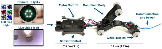
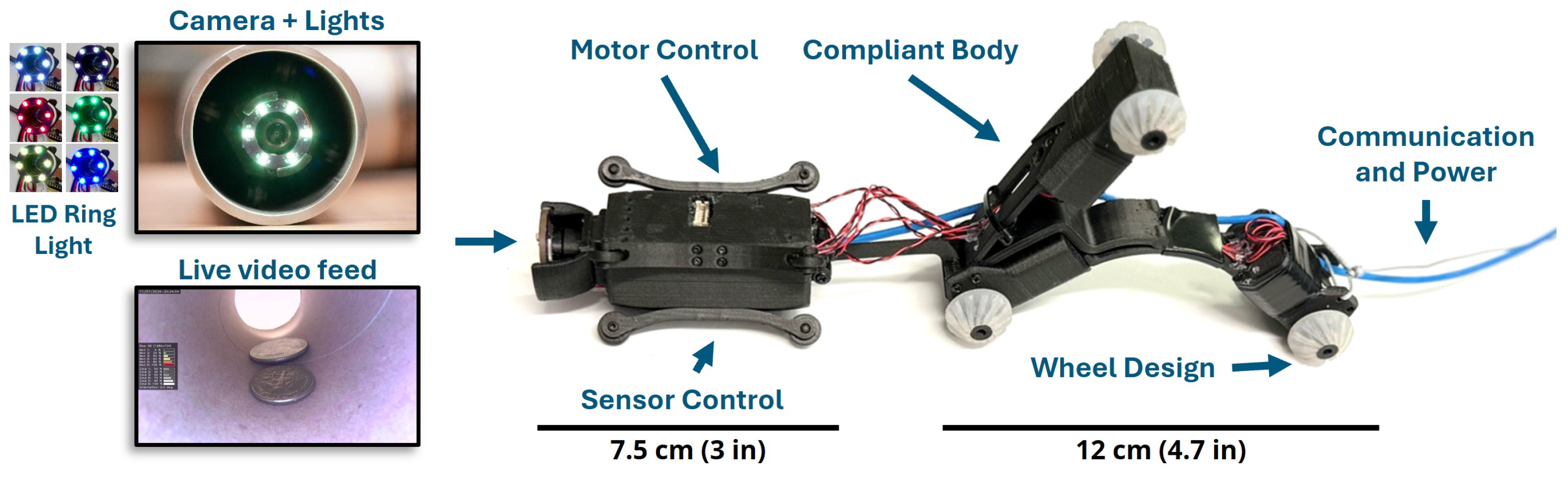
In this work, we present the Self-Propelled Interior Inspector for NDT Examination (SPIINE—pronounced “spine”), an innovative, flexible in-pipe inspection robot (see Figure 1) designed to address the significant challenges imposed by size constraints, tight bends, and long pipe lengths. Specifically, SPIINE demonstrates the following capabilities:

Figure 1. Self-Propelled Interior Inspector for NDT Examination (SPIINE) with flexible chassis for navigating tight bends with an onboard IMU, high-resolution video camera, and tether for power/data transmission.

• Access and navigate through a 53 mm ID pipe;
• Traverse tight 90° elbows (radius of curvature as small as 76 mm (3 in));
• Transmit power and data (including high-resolution video) over long tethers (≥110 m);
• Generate pull forces over eight times the weight of the robot in straight steel pipe to support towing of NDT sensor payloads.

Although existing in-pipe robots have demonstrated a wide range of locomotion and adaptation strategies, most are intended for larger pipe diameters, require active reconfiguration or orientation control, do not report tight-elbow traversal at arbitrary roll orientations, or do not quantify available pull force for payload towing. Thus, these systems only address a subset of the challenging requirements outlined above. Table 1 summarizes representative research and commercial pipe-inspection systems targeted for small pipe diameters ≤102 mm (4 in) and highlights the capabilities and limitations of existing systems. While many reported systems demonstrate promising locomotion or sensing capabilities, practical deployment factors such as tow force, travel distance, and tether length are often not explicitly considered.

Table 1. Representative research and commercial pipe-inspection systems targeted for small-diameter pipes, ≤102 mm (4 in), organized by increasing pipe diameter. Highlighted rows indicate systems compatible with 53 mm (2 in) pipe diameters or smaller. Checkmarks (✓) and crosses (×) indicate whether the listed system satisfies or does not satisfy the corresponding performance metric, respectively.

Category	System/Author	Locomotion Method	Pipe Diameter	Tight Elbows *	Curves **	Tested Distance, Tether (m) ***	Max Speed (mm/s)	Tow Force (N)	Sensor Modality	Notes and Limitations
Research	Micro inspection robot, Suzumori et al. [19]	Wheeled locomotion	25 mm (1 in)	×	✓	$1.5^{+}$, 1.5	6	1	Camera; Micro hand	Low payload capacity limits practical deployment.
Commercial	SeeSnake microReel, RIDGID [20]	Manual push camera with semi-rigid cable	40–101 mm (1.5–4 in)	✓	✓	30, 30	Manual	Not Applicable	Camera	Inspection distance and maneuverability are limited by pipe bends and inability to actively navigate junctions.
Commercial	Endo CRXS-50 Pipe Crawler, Spectis Robotics [21]	Wheeled locomotion	50–55 mm (2–2.1 in)	✓	✓	20–30, 20–30	66.67	35 (Traction Force)	Camera	Inspection distance and maneuverability are limited by the number of pipe bends.
Commercial	Versatrax I-Series/ VT-50, Eddyfi Technologies [22]	Tethered tracked or magnetic crawler, depending on configuration	50–100 mm (2 in)	×	✓	60, 100	31.67	45	Camera	Rigid chassis length restricts mobility through tight elbows.
Research	SPIRA, Kamezaki et al. [23]	Spiral wheeled locomotion	52–64 mm (2–2.5 in)	✓	✓	30, 30	100	3.929 (Traction Force)	None	Current lack of sensors is not ideal for inspection applications.
This Work	SPIINE	Wheeled with compliant body	53 mm (2 in)	✓	✓	≥60, 110	12.83	16.5	Camera; IMU	Compliant body for long tethered operation and navigating tightelbows.
Research	Micro-robot “Joey”, Nguyen et al. [24]	Wheel-legs micro-crawler	75–200 mm (3–8 in)	✓	✓	$2.7^{+}$, Tetherless	70	Low; NS ****	IMU; Encoder; Time-of-flight range sensors; MEMS microphone; Camera	Complex for miniaturization. Mainly tested in 150mm diameter pipe.
Research	Differential-drive in-pipe robot, Roh and Choi [25]	Wheeled differential- drive modules pressed against the pipe wall	80–100 mm (3.1–3.9 in)	✓	✓	$4.7^{+}$, 4.7	150	9.8 (Traction Force)	Camera	Difficult to miniaturize to 2 in pipes because of actuator, wheel, and steering- volume constraints.
Research	AIRo 5.2 articulated wheeled robot, Kakogawa et al. [26]	Articulated wheeled locomotion	100–127 mm (4–5 in)	✓	✓	26, 26	80	202 (Traction Force)	Joint angle sensing	Advanced mobility for T-branches; mechanical complexity makes miniaturization challenging.

* Tight Elbows are defined as ${90}^{\circ }$ bends with a radius of curvature, measured from the center point of the arc to the centerline axis of the pipe, equivalent to ≤1.5 times the internal pipe diameter. ** Curves refer to bends with a radius of curvature equivalent to >1.5 times the internal pipe diameter. *** Tested Distances are based on in-pipe testing. Tether Length is based on the length of the tether used during testing and is a repeated value of the Tested Distance if it is not specified in the literature. + Values were approximated based on images of the experimental setups shown, since no value was explicitly mentioned in the literature. **** NS: Not specified in the literature.

Key contributions of this work include the integrated design and validation of a passively compliant six-wheeled architecture that combines small-diameter access, tight-elbow traversal from a variety of entry angles (roll orientations) spanning 360°, long-distance (>100 m) tether operation, and high tractive force generation relative to robot weight, together with an analytical stiffness-to-pull-force modeling framework that has been validated with hardware experiments.

In Section 2, we describe the robot design, including key system requirements and the mechanical design of the robot’s drivetrain elements and flexible chassis. In Section 3, we present an analytical model of the robot’s flexural stiffness that characterizes deflection and reaction force generation, which directly contributes to pull force generation. In Section 4, we present experimental results from a hardware prototype, including stiffness-model validation, pull-force measurements, bend-traversal tests, long-distance traversal, and power/data transmission. Finally, in Section 5 we summarize our conclusions and discuss future work.

2. Pipe Inspection Robot Design

This Section summarizes the design requirements, drivetrain design, compliant chassis architecture, and electronics implementation for the SPIINE prototype. The design process was driven by the combined need to fit within 53 mm ID pipe, traverse tight elbows, generate sufficient tractive force for payload towing, and maintain power and data transmission over long tether lengths. The following subsections first define the target requirements, then describe the mechanical and electronic design choices used to meet those requirements.

2.1. Key Design Considerations

Designing a functional in-pipe inspection robot requires consideration of several key performance and reliability requirements. For SPIINE, we targeted the ability to:

1.

Access pipes with a 53 mm (2 in) ID;

2.

Navigate multiple bends with radii of curvature ≤0.91 m (3 ft), including at least one 90° elbow with a 76 mm (3 in) radius;

3.

Traverse $\ge 100$ m (328 ft) at 0.3+ m/min (1+ ft/min);

4.

Support additional sensor payloads (onboard or towed);

5.

Operate for several hours with a 100 W maximum power budget to reduce tether size;

6.

Provide high-resolution video with adjustable illumination for visual inspections.

2.2. Pull Force Requirements

To effectively traverse long distances while also transporting a sensor payload, the robot must generate sufficient pull force to tow the payload, especially as the weight and resistance of the tether increase with distance. At a minimum, our pipe inspection robot must generate enough pull force to counteract any resistance induced by its tether. Ideally, the system will generate sufficient overhead force to support pulling additional NDT sensor payloads as well. To determine a conservative (upper limit) estimate of the tether resistance force, we measured the force required to drag an Ethernet tether cable through a 90° elbow (76 mm radius) and along various lengths of a flat asphalt surface.

This pull force measurement represents a tight bend constraint at the entry point of a pipe, along with tether friction against the inner surface of the pipe. Based on these tests, we set the pull-force requirement to 12 N (2.7 lb), corresponding to 50% force overhead beyond the measured 8 N of resistance produced by a 30 m (100 ft) tether.

2.3. Drivetrain Design

We considered both wheel and track options for actuating the robot and found that a pair of wheels, each driven by a separate motor, was able to generate slightly more pull force than a track driven by two motors and also introduced fewer potential failure points. Thus, we opted to use individual motor-driven wheels for propulsion with an effective contact radius (radial distance from motor output shaft axis to wheel contact point) of 6.35 mm (0.25 in). To achieve a target robot pull force of 12 N distributed across six wheels, each wheel must generate 2 N of force, and thus each motor must produce a torque $\tau =Fr=2\times 6.35=12.7$ N·mm. The six-wheel load distribution used here for motor sizing should be interpreted as a first-order design estimate; during operation, individual wheel normal forces may vary with chassis deflection, pipe geometry, and robot orientation, so the pull-force model and experiments evaluate the aggregate tractive capability of the robot rather than equal load sharing at each wheel.

Next, we evaluated speed, torque, and power consumption across dozens of motor form factors (6–12 mm diameters), gear ratios (5:1–1000:1), and drive voltages (3–12 V). Although a 6 mm motor was initially attractive for its compact size, its marginal continuous torque and fragile plastic planetary gears led us to select the larger, more reliable Precision Mini Drives NFP-GW12TRS-N20 motor to meet pull-force requirements. This 12 V, 12 mm micro DC motor uses metal gears with a 603:1 gear ratio, provides 78 N·mm rated continuous torque (196 N·mm stall), and has a rated load current of ≤0.15 A. Based on these specifications, we established an effective continuous current limit of 0.25 A, yielding a 3 W per-motor power budget ($P=IV=0.25\times 12=3$) and a conservative (since the motors are not expected to experience maximum load conditions continuously) total power budget of 18 W for the six-wheeled robot.

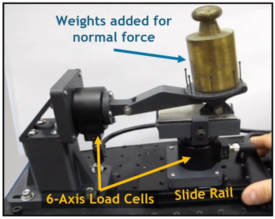
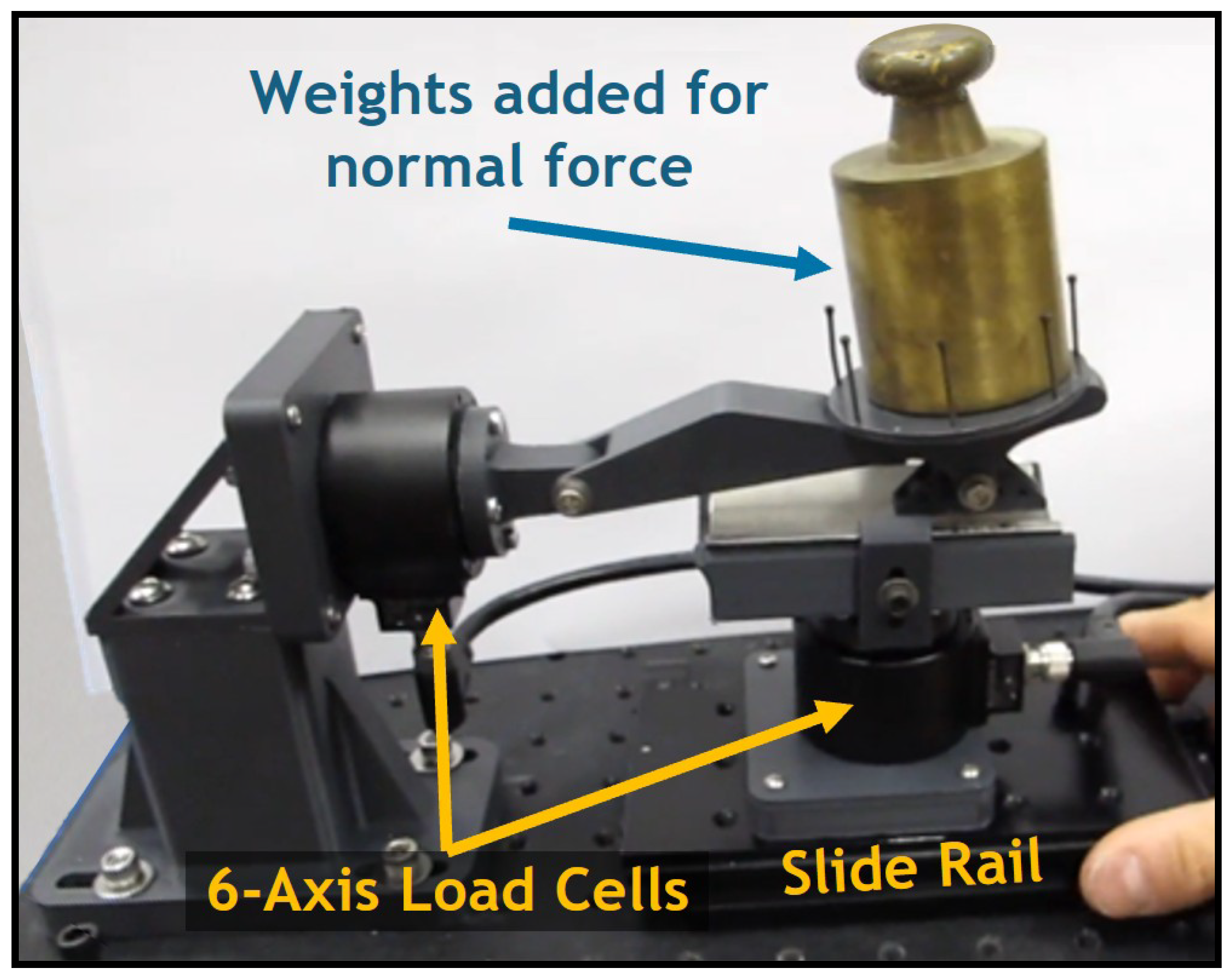
To complete the drivetrain design, we performed characterization tests to identify the coefficient of friction between a steel pipe section and two candidate wheel materials: Dragonskin silicone rubber with Shore 30A hardness, and a 3D-printable thermoplastic polyurethane (TPU). We used calibrated weights to apply a constant normal force to a thin slab of material resting on an instrumented test pipe section and pulled the pipe section along a linear rail to measure the resulting pull force transmitted through the material via friction (see Figure 2). Based on this comparison, we selected the silicone as our wheel material with a measured coefficient of friction of $\mu \approx 1.2$, compared to only $\approx 0.4$ for the TPU.

Figure 2. Instrumented testbed for measuring friction and force generation on steel pipe.

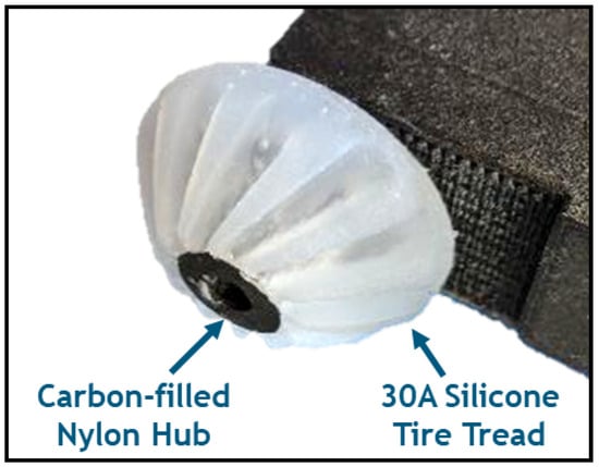
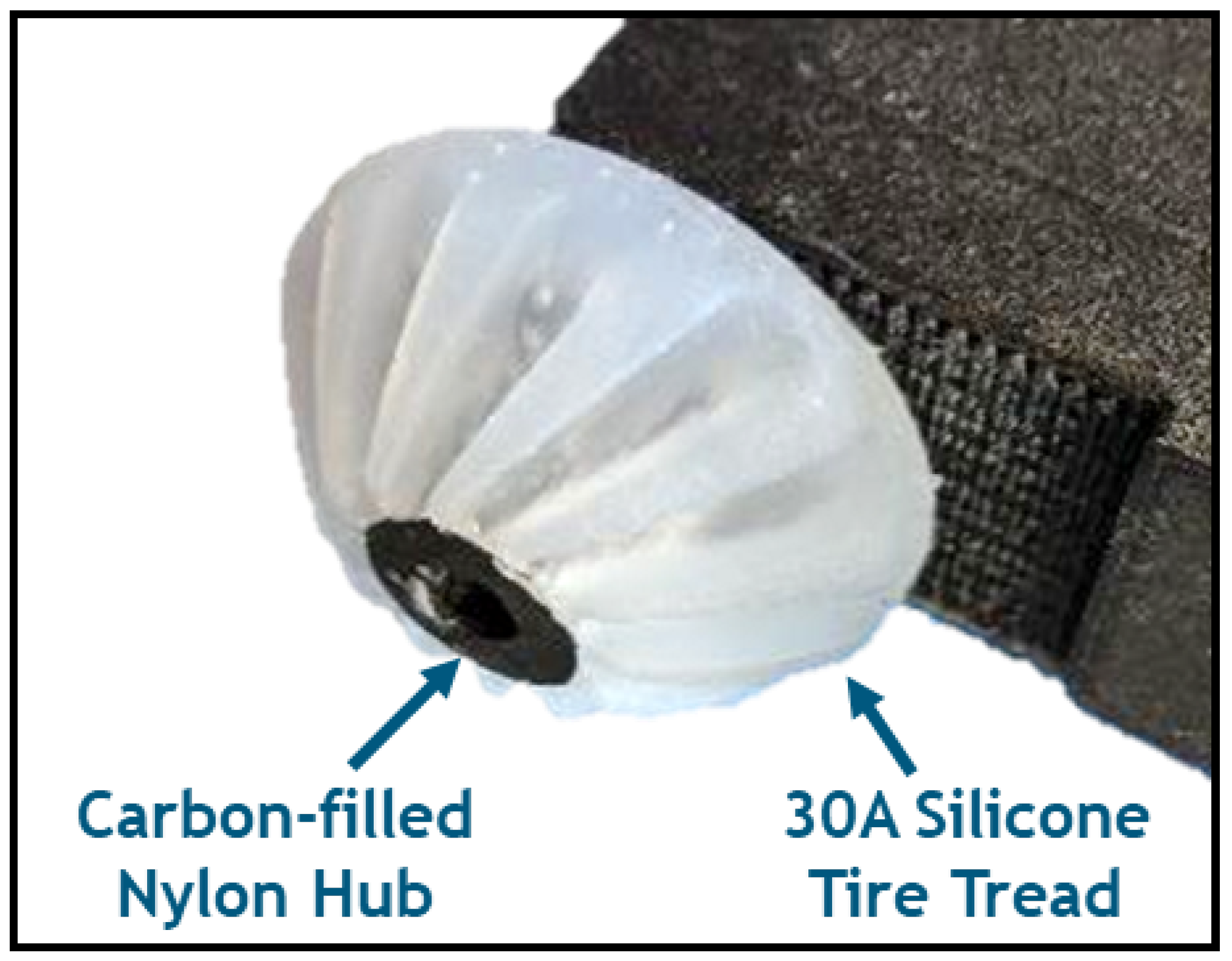
To construct each wheel, we created a hybrid design consisting of a carbon-filled nylon hub surrounded by silicone molded into a curved shape that matches the inner curvature of the pipe, with ridges to help improve traction (see Figure 3). The nylon hub also includes internal engagement features to improve mechanical interlock with the molded silicone tread and reduce the likelihood of slip or delamination at the hub–tread interface. Across the prototype test campaigns reported here, including repeated bend traversal and long-distance driving, we did not observe silicone delamination or cracking. Extreme vehicle loading conditions, such as the fully inverted elbow orientation described in Section 2.4, are expected to be rare and transient during normal operation; nevertheless, more comprehensive wheel endurance testing under repeated high-load elbow traversal is planned for future work.

Figure 3. Hybrid wheel design for the in-pipe inspection robot.

Noting that wheel tread geometry can increase the contact friction above the interfacial coefficient of friction [27,28], we attached an assembled wheel to the testbed shown in Figure 2 and used a similar procedure to that described above to measure the coefficient of friction of the final wheel design: $\mu \approx 2.1$.

We also decided to use the same carbon-filled nylon material (Onyx from Markforged, Waltham, MA, USA) to 3D-print all of the other robot structural components as it exhibits excellent strength, toughness and wear resistance.

2.4. Modular, Flexural Drive Body Design

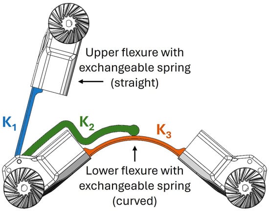
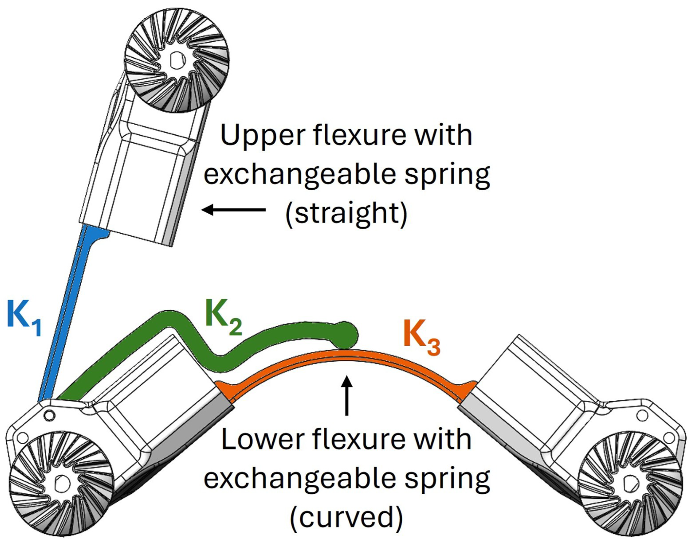
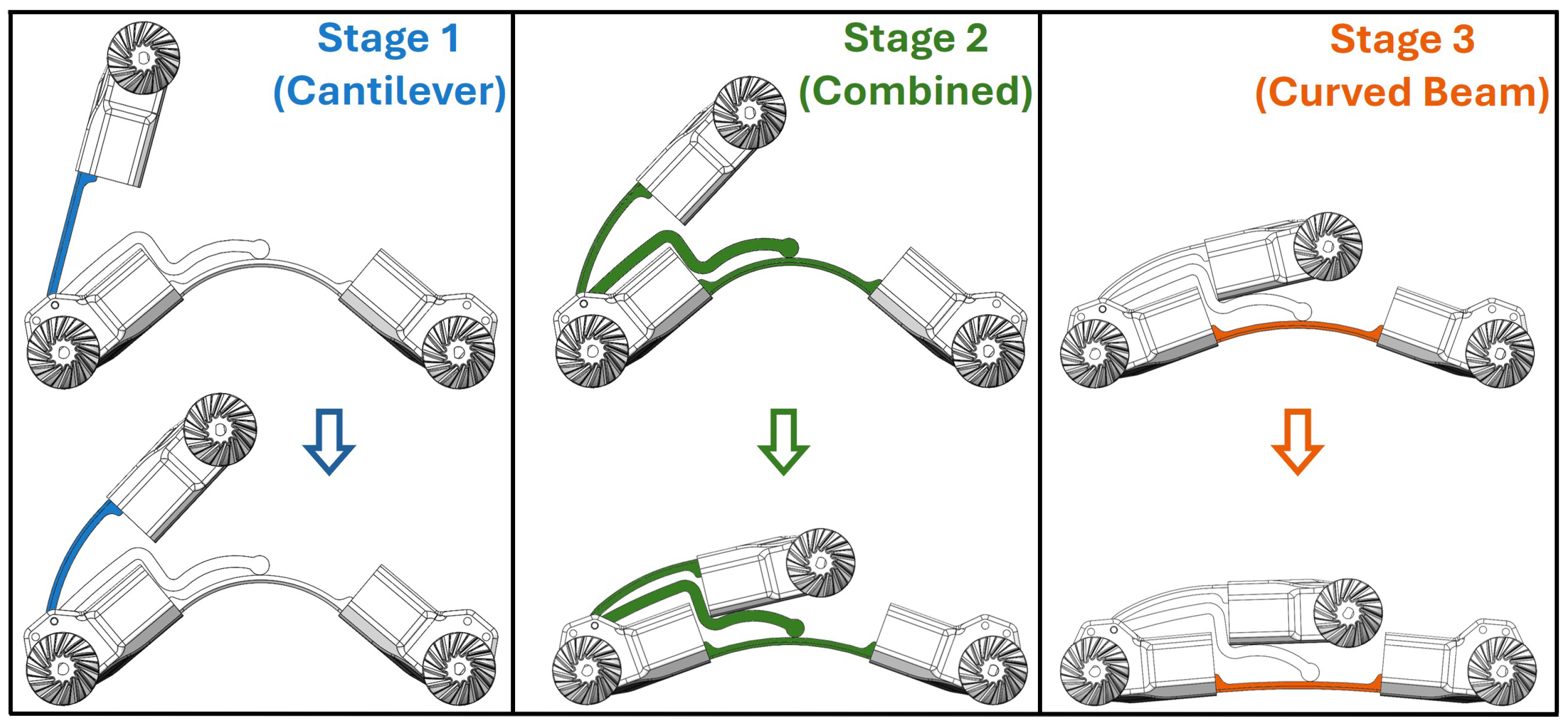
After completing the motor selection and wheel design, we employed a rapid iterative design process to build and test prototypes within pipes, which enabled quick identification of component strengths and weaknesses. Through several iterations with hardware prototypes, we developed a modular, multi-axis flexural drive body (shown in Figure 4 and Figure 5) that can traverse the targeted 90° elbows with a radius of 76 mm. This design incorporates two flexural body springs—one straight (shown in blue), and one curved (shown in orange)—that can be exchanged to adjust the normal force applied in the pipe. An intermediate adapter plate (shown in green in Figure 4) is rigidly attached to the cantilever bar (manufactured as one piece) and transmits force between the upper and lower flexures as the body is compressed.

Figure 4. Multi-axis flexural drive body design with exchangeable straight and curved spring sections (blue and orange). An adapter plate (green) transmits force between the upper and lower flexures. See Section 3 for a description of $K_1$, $K_2$ and $K_3$.

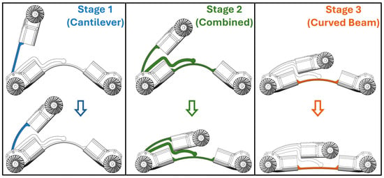
Figure 5. Three progressive stages of drive body compression with active stiffness components highlighted for each stage.

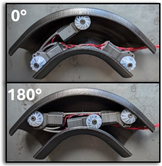
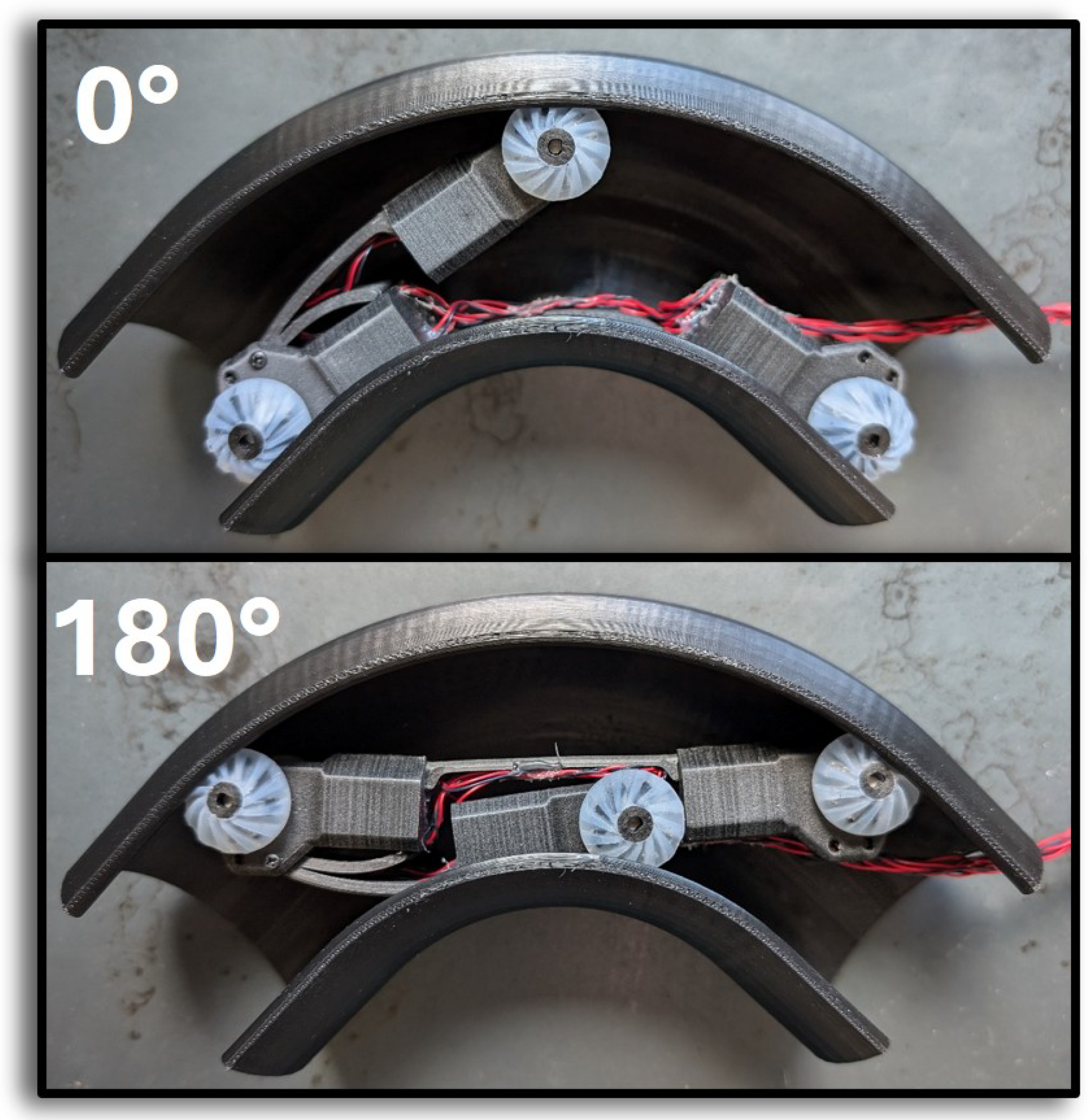
As shown in Figure 6, the body design has a “natural” elbow entry orientation with 0° relative rotation between the body’s plane of curvature and the elbow’s plane of curvature that produces minimal internal twisting and resistance. However, the robot is capable of navigating the elbow in a variety of orientations spanning 360°, including fully inverted as shown at the bottom of Figure 6. Furthermore, its multi-axis flexibility allows the chassis to passively accommodate variations in bend-entry orientation and pipe geometry without active steering or orientation control.

Figure 6. SPIINE robot traversing 90° elbow in the “natural” 0° orientation relative to the elbow’s plane of curvature (top) and with a 180° (inverted) rotation (bottom).

2.5. Electronics, Command, and Control

To enable parallel iteration on electronics and the flexural drive body (see Figure 1), we used a separate electronics trolley (to be integrated into the drive body in future iterations). We designed custom printed circuit boards (PCBs) for (i) pulse-width modulation (PWM) control of six motors with hardware current limiting and (ii) camera/lighting control and sensor processing, including IMU and motor-current feedback. Images and robot telemetry are transmitted to a host computer via Ethernet using user datagram protocol (UDP), with adjustable illumination and selectable image/video resolution (up to $1920\times 1080$ video and $2560\times 1920$ images). A Robot Operating System (ROS2 Humble [29])-based interface with OpenCV [30] provides live viewing, logging, and operator control via gamepad/keyboard.

2.6. Image Resolution for Inspections

Utilizing our custom PCB for image capture and streaming to the host computer via UDP, we are able to achieve real-time video streaming at multiple configurable resolutions; see Table 2 for associated pixel counts, frames per second (FPS) and latency achieved for each resolution. Latency here is defined as the "glass-to-glass" time between when an event occurs (e.g., a light turns on) and when the event is observed on the user’s display. The observed latency for the lower-resolution streaming modes was sufficiently low for operator-guided inspection, while the highest-resolution QSXGA mode is primarily intended for still-image capture or slow inspection rather than low-latency teleoperation.

Table 2. SPIINE’s available image resolutions, with associated pixel counts, frame rates in frames per second (FPS), and latencies.

Resolution	Pixels	Rate (FPS)	Latency (ms)
VGA	$640\times 480$	22 *	160
HD	$1280\times 720$	25 *	160
FHD	$1920\times 1080$	6	290
QSXGA **	$2560\times 1920$	N/A	≈1000

* Low-level image sensor firmware is optimized for specific configurations; thus, frame rate is not always higher for lower resolutions. ** High-resolution QSXGA is available for snapshots only.

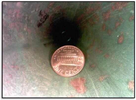
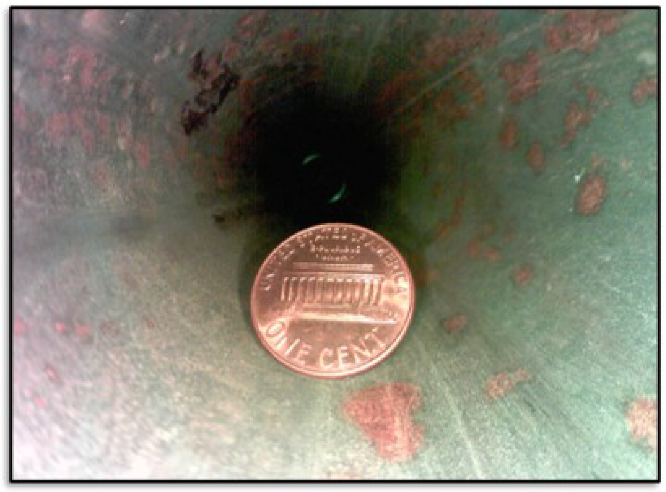
We implemented a snapshot capability so the vehicle can be stopped at a specific region of interest to capture a clear, higher-resolution image for inspection without any concerns about motion blur due to translational or rotational motion. Figure 7 shows an example high-resolution image ($2560\times 1920$ pixels) captured inside a 53 mm (2 in) diameter pipe, with a United States penny (19.05 mm in diameter) placed in the pipe as a size reference. The penny is ≈485 pixels across, corresponding to a resolution of $25.5$ pixels per mm or 39.3 μm per pixel—this allows operators to observe very small features and/or flaws during pipe inspections.

Figure 7. Example high-resolution ($2560\times 1920$ pixels) image captured inside 53 mm (2 in) pipe. A 19.05 mm diameter United States penny is placed in the pipe as a size reference. The penny is ≈485 pixels across, corresponding to a resolution of $25.5$ pixels per mm or 39.3 μm per pixel.

2.7. Sensor Payload Attachment

To support towing additional NDT sensors (separate from the primary tether), we included a clamping feature at the bottom of the robot that accommodates cables with diameters up to 15.9 mm (5/8 in).

3. Deflection and Stiffness Modeling

The amount of pull force the robot can generate at any instant depends directly on the normal force pressing the wheels against the pipe’s inner surface and the coefficient of friction for those points of contact. For straight sections of the pipe, this normal force will remain constant. However, as the robot traverses the elbow geometry, the normal force may vary depending on the body’s orientation relative to the elbow. For example, the robot body experiences minimum compression (and thus minimum normal force) at the 0° “natural” orientation relative to the elbow, and maximum compression/normal force in the 180° orientation as shown in Figure 6. To estimate the normal force applied at any given orientation or configuration within a pipe, we developed a model of the body’s stiffness relative to the vertical displacement imposed by the pipe’s inner geometry. Model assumptions include quasi-static loading, symmetric wheel contact about the pipe centerline, Coulomb friction, and rigid motor housings relative to the flexural elements.

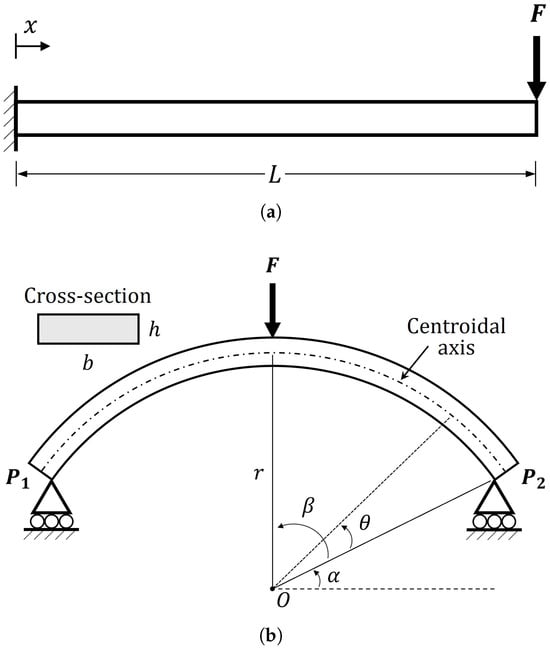
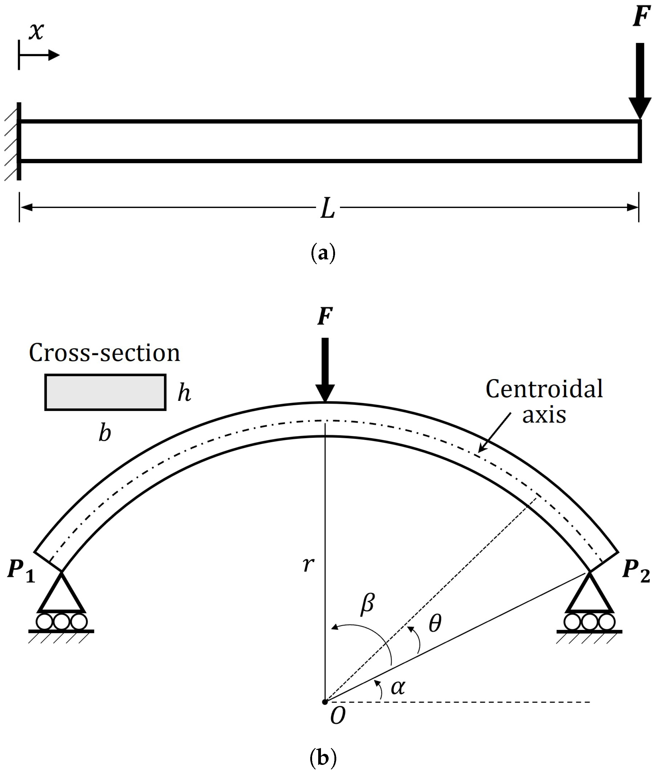
Our stiffness model utilizes the cantilever and curved beam structures shown in Figure 8a,b to approximate the effective structural stiffness of the robot body (compare to Figure 4).

Figure 8. Beam structures that approximate the SPIINE robot’s primary sources of normal/vertical stiffness. (a) Cantilever beam representing the robot’s upper flexure. F is the normal force on wheels applied against upper pipe surface. (b) Simply supported curved beam (roller–roller) representing the robot’s lower flexure. Loading force F is normal force transmitted via adapter plate from upper chassis, r is the radius of curvature, and $P_1$ and $P_2$ are the ground contact points.

The chassis behaves approximately as a two-element compliant structure with an upper cantilever and a lower curved beam. As vertical compression increases, the vertical force shifts toward the center of the robot and load transfer through an adapter plate produces three effective vertical stiffness stages as shown in Figure 5: (1) cantilever-dominated (with stiffness $K_1$), (2) series-combination region (with stiffness $K_2$), and (3) curved-beam-dominated (with stiffness $K_3$).

3.1. Application of Castigliano’s Theorem

Assuming the vehicle body is in equilibrium with elastic deformation inside a 53 mm (2 in) ID pipe, we model the downward displacement of the upper wheels using Castigliano’s theorem: $\delta =\partial U/\partial F$, where $\delta$ is the work-absorbing displacement associated with an external load F and U is the strain energy of the body expressed in terms of the external load [31].

Considering the superimposed contributions of axial loading, torsion and bending, and since the applied load F is not a function of position, the partial derivative of strain energy with respect to the applied load can be written as:

$${\displaystyle \frac{\partial U}{\partial F}}={\int }_0^L{\displaystyle \frac{F}{EA}}{\displaystyle \frac{\partial F}{\partial F}}dx+{\int }_0^L{\displaystyle \frac{T}{GJ}}{\displaystyle \frac{\partial T}{\partial F}}dx+{\int }_0^L{\displaystyle \frac{M}{EI}}{\displaystyle \frac{\partial M}{\partial F}}dx$$

(1)

where L is the length of the beam, $dx$ is an infinitesimal change in distance along the X-axis, F is the applied load, E is the tensile or flexural modulus of the beam material, $A=bh$ is the cross-sectional area of the rectangular beam (see Figure 8b), T is the applied torque about the X-axis, G is the shear modulus of the material, J is the polar moment of inertia, M is the bending moment, and $I=b{h}^3/12$ is the area moment of inertia about the centroidal axis.

For a cantilever beam, the axial and torsional loading terms can be ignored, and after integration over the length of the beam, this simplifies to:

$$F=\delta ·{\displaystyle \frac{3EI}{L^3}}$$

(2)

where F is the applied normal force.

For a simply supported (roller–roller) curved beam with a single applied load at the center (see Figure 8b), we convert to polar coordinates and integrate over the arc length, replacing $dx$ with $rd\theta$, and get:

$${\displaystyle \frac{\partial U}{\partial F}}={\int }_0^{\beta }{\displaystyle \frac{F}{EA}}{\displaystyle \frac{\partial F}{\partial F}}rd\theta +{\int }_0^{\beta }{\displaystyle \frac{T}{GJ}}{\displaystyle \frac{\partial T}{\partial F}}rd\theta +{\int }_0^{\beta }{\displaystyle \frac{M}{EI}}{\displaystyle \frac{\partial M}{\partial F}}rd\theta$$

(3)

where r is the radius of curvature of the beam’s centroidal axis, $d\theta$ is an infinitesimal change in angle of the radius vector, $\beta$ is one half of the angle subtended by the beam arc, and the origin of $\theta$ is the vector between the origin of the beam’s centroidal arc O and the ground contact point $P_2$. The angle $\alpha$ from the horizontal to ${\theta }_0$ is:

$$\alpha ={\displaystyle \frac{\pi }{2}}-\beta .$$

(4)

Again, in this case, we can ignore torsional loading, and since the radius of curvature is much greater than the thickness of the beam ($r/h>10$), the contribution to deflection from the axial load is also negligibly small compared to that from the bending moment, and thus we need only consider the bending component [32].

To account for bending, we define the bending moment $M\left(\theta \right)$ as the product of the ground reaction force at $P_2$ ($F/2$) and the moment arm to the point of integration, computed as the horizontal offset from $P_2$ to the point on the curve offset by the angle $\theta$:

$$\begin{array}{cc}\hfill momentarm& =r·cos\left(\alpha \right)-r·cos(\alpha +\theta )\hfill \\ \hfill & =r·\left[cos\left({\displaystyle \frac{\pi }{2}}-\beta \right)-cos\left({\displaystyle \frac{\pi }{2}}-\beta +\theta \right)\right]\hfill \\ \hfill & =r·\left[sin\left(\beta \right)-sin(\beta -\theta )\right]\hfill \\ \hfill & =2r·sin\left({\displaystyle \frac{\theta }{2}}\right)·cos\left(\beta -{\displaystyle \frac{\theta }{2}}\right)\hfill \end{array}$$

(5)

Thus, we obtain $M\left(\theta \right)$ and its partial derivative with respect to the applied load F as follows:

$$\begin{array}{cc}\hfill M\left(\theta \right)& =F·r·sin\left({\displaystyle \frac{\theta }{2}}\right)·cos\left(\beta -{\displaystyle \frac{\theta }{2}}\right)\hfill \\ \hfill {\displaystyle \frac{\partial M}{\partial F}}& =r·sin\left({\displaystyle \frac{\theta }{2}}\right)·cos\left(\beta -{\displaystyle \frac{\theta }{2}}\right)\hfill \end{array}$$

(6)

Noting symmetry, we integrate over half the curve length ($\beta$) and multiply by two. Thus, the full deflection equation for the curved beam becomes:

$$\delta =2{\int }_0^{\beta }{\displaystyle \frac{F{r}^3}{EI}}·si{n}^2\left({\displaystyle \frac{\theta }{2}}\right)·co{s}^2\left(\beta -{\displaystyle \frac{\theta }{2}}\right)d\theta$$

(7)

After integration and solving for F, we obtain:

$$F=\delta /\left[\left({\displaystyle \frac{r^3}{EI}}\right)·\left({\displaystyle \frac{\beta }{2}}-sin\left(\beta \right)+{\displaystyle \frac{3}{8}}sin\left(2\beta \right)-{\displaystyle \frac{\beta }{4}}cos\left(2\beta \right)\right)\right]$$

(8)

3.2. Combined Body Stiffness

From Equations (2) and (8), we can extract the equivalent vertical stiffness of the cantilever and curved beam stages of the body deflection as $K_1$ and $K_3$, respectively, to fit the form of Hooke’s law: $F=Kx$ as follows:

$$\begin{array}{cc}\hfill K_1& ={\displaystyle \frac{3EI}{L^3}} \hfill \end{array}$$

(9)

$$\begin{array}{cc}\hfill K_3& =1/\left[\left({\displaystyle \frac{r^3}{EI}}\right)·\left({\displaystyle \frac{\beta }{2}}-sin\left(\beta \right)+{\displaystyle \frac{3}{8}}sin\left(2\beta \right)-{\displaystyle \frac{\beta }{4}}cos\left(2\beta \right)\right)\right]\hfill \end{array}$$

(10)

To obtain the vehicle stiffness during the intermediate stage where the upper cantilever is fully engaged but the lower curved beam is only partially engaged by the adapter plate, we combine $K_1$ and $K_3$ in series, with a modifier $\eta \in [0,1]$ applied to $K_3$ to account for partial engagement. This yields:

$$K_2={\displaystyle \frac{K_1·\eta K_3}{K_1+\eta K_3}}$$

(11)

Now, for any given vertical displacement $\delta$, we can compute the corresponding vertical force exerted by the robot’s flexural drive body with:

$$\begin{array}{c}\hfill F_v\left(\delta \right)=\left\{\begin{array}{cc}{K}_1·\delta \hfill & \mathrm{for}\delta \le {\delta }_1\hfill \\ K_2·{\delta }_{1r}+F_v\left({\delta }_1\right)\hfill & \mathrm{for}{\delta }_1<\delta \le {\delta }_2\hfill \\ K_3·{\delta }_{2r}+F_v\left({\delta }_2\right)\hfill & \mathrm{for}\delta >{\delta }_2\hfill \end{array}\right.\end{array}$$

(12)

where ${\delta }_1$ is the deflection at which the lower flexure starts to be engaged, ${\delta }_2$ is the deflection at which the upper flexure is no longer engaged (upper motor housing in full contact with adapter plate), ${\delta }_{1r}=\delta -{\delta }_1$ and ${\delta }_{2r}=\delta -{\delta }_2$ are the deflections relative to ${\delta }_1$ and ${\delta }_2$, respectively, and $K_1$, $K_2$, and $K_3$ are the stiffnesses defined in Equations (9)–(11).

The analytical stiffness and force terms in Equations (9)–(12) provide the primary model used to relate chassis geometry, vertical reaction force, and pull-force capability. For the lower curved flexure, finite-deflection effects introduce geometric softening that is not captured by the nominal linear-beam expression for $K_3$. Therefore, the numerical predictions in Section 4 apply an FEA-informed correction factor to produce $K_{3_{corr}}$, defined in Section 4.1.1, which adjusts the nominal analytical value to account for geometric-nonlinearity effects.

3.3. Radius of Curvature

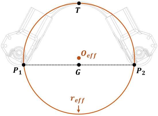
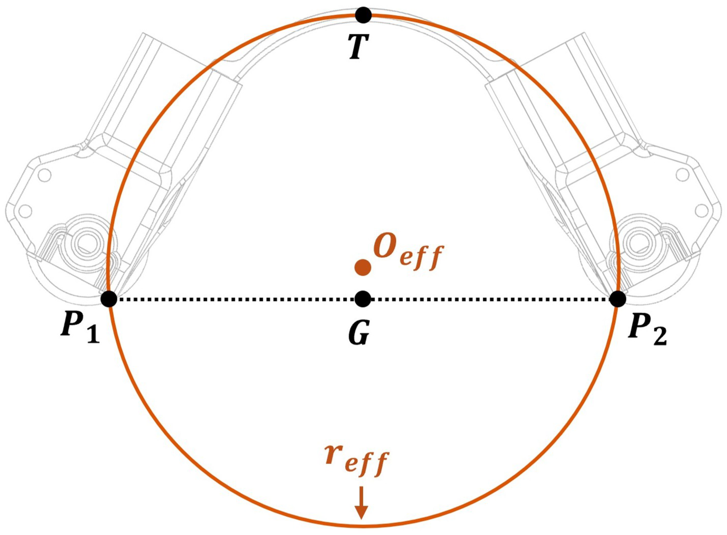
As we worked with prototypes of the robot constructed with a nylon-based 3D-printed material, we found that the robot curvature settles to a repeatable steady state after several compression cycles associated with entering and exiting a pipe. Because the lower motor housings can be treated as rigid bodies relative to the flexural spring, deformation occurs primarily in the spring while the rigid housings impose geometric boundary conditions on the overall body curvature. We therefore developed the method below (illustrated in Figure 9) to compute an effective radius of curvature, $r_{eff}$, for the flexural drive body after break-in.

Figure 9. Definition of the effective radius of curvature ($r_{eff}$, shown as orange circle with origin $O_{eff}$) for the lower flexure based on vehicle body contact with ground (dashed line) after break-in for computing $K_3$.

We define $r_{eff}$ as the radius of a curve defined by the highest point of the curved spring’s centroidal axis T and the two points of ground contact $P_1$ and $P_2$ as shown in Figure 9.

We calculate $r_{eff}$ based on two dimensions that can be readily measured on a hardware prototype: $w_{gnd}$, which is $|\overline{P_1{P}_2}|$ (ground contact width), and h, which is $|\overline{GT}|$ as shown in Figure 9. Then, we can use the arc radius formula derived from the intersecting chords theorem [33] to obtain:

$$r_{eff}={\displaystyle \frac{w_{gnd}^2}{8h}}+{\displaystyle \frac{h}{2}}$$

(13)

To compute the equivalent stiffness $K_3$ of the curved beam body deflection in Equation (10), we must also determine $\beta$ as follows. First, we obtain $\alpha$ noting the geometry shown in Figure 8b as:

$$\alpha =atan2\left(r_{eff}-h,{\displaystyle \frac{w_{gnd}}{2}}\right).$$

(14)

Then, we substitute Equation (14) into Equation (4) and solve for $\beta$ (half the effective angle subtended by the robot’s flexural drive body) as:

$$\beta ={\displaystyle \frac{\pi }{2}}-atan2\left(r_{eff}-h,{\displaystyle \frac{w_{gnd}}{2}}\right).$$

(15)

Using the $atan2$ function allows for $O_{eff}$ to be on or below $\overline{P_1{P}_2}$ ($\beta \le \pi /2$ as shown in Figure 8b) or above $\overline{P_1{P}_2}$ ($\beta >\pi /2$, as shown in Figure 9).

3.4. Pull Force Estimation from Pipe Geometry

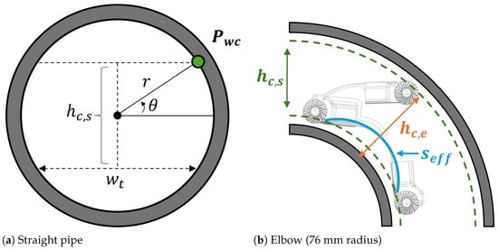
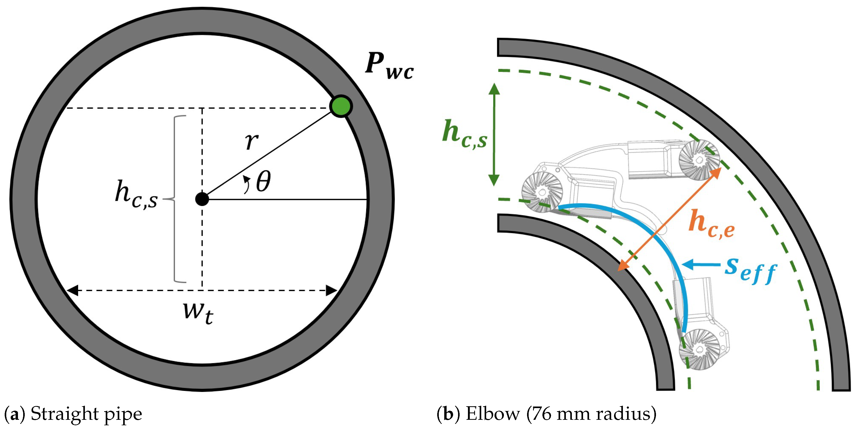
The maximum pull force that SPIINE can generate is governed by the available friction force at the wheel–pipe contacts. This friction force depends on (i) the robot’s body deflection imposed by pipe geometry, (ii) the resulting chassis reaction force predicted by the stiffness model in Section 3.2, and (iii) the wheel–pipe coefficient of friction. We derive equations below to estimate pull force for two key cases relevant to our design: (i) straight pipe and (ii) the minimum-compression condition in a 90° elbow (0° orientation in Figure 6) as depicted in Figure 10.

Figure 10. Cross-sections showing compressed robot dimensions in straight and elbow segments of 53 mm ID pipe. In (a), $w_t$ is the vehicle track width, r is the inner radius of the pipe, and $\theta$ is the angle to the wheel contact point $P_{wc}$ (green circle). The green and orange lines in (b) depict the compressed height of the vehicle in straight and elbow pipe sections—$h_{c,s}$ and $h_{c,e}$, respectively—and the blue curve in (b) denotes the effective arc length $s_{eff}$ of the lower flexure between wheel contact points.

3.4.1. From Pipe Geometry to Vertical Body Deflection

Let $h_0$ denote the robot’s uncompressed height measured between the lower and upper wheel contact points. We compute the robot’s compressed height from geometry for the two pipe configuration cases shown in Figure 10 as

$$h_c=2rsin\left(\theta \right),$$

(16)

and the imposed vertical deflection is: $\delta =h_0-h_c$.

3.4.2. From Deflection to Vertical Reaction Force

Using the piecewise stiffness model developed in Section 3.2, we compute the vertical reaction force $F_v$ produced by the compliant chassis with Equation (12).

3.4.3. From Vertical Reaction Force to Normal Force at Wheel Contacts

At each wheel contact, the normal force is the component of the vertical reaction force along the local pipe normal direction. Approximating symmetric contact about the pipe centerline, the normal force at the contact point is $F_n=F_{v}sin\left(\theta \right)$, where $\theta$ is the polar angle from the horizontal to the wheel contact point $P_{wc}$ (see Figure 10a). For a straight pipe with inner radius r and track width $w_t$ (horizontal distance between the robot’s wheels), we can compute $\theta$ as

$$\theta =co{s}^{-1}\left({\displaystyle \frac{w_t/2}{r}}\right).$$

(17)

3.4.4. From Normal Force to Pull Force

Assuming Coulomb friction with coefficient $\mu$, the available pull force scales with normal force. In this work, we estimate total pull force as the friction force corresponding to the normal force at the upper contacts plus the corresponding reaction at the lower contacts, yielding

$$F_{pull}\approx 2\mu F_v\left(\delta \right)sin\left(\theta \right),$$

(18)

where $F_v\left(\delta \right)$ is given by Equation (12) and $\delta =h_0-h_c$ is obtained from pipe geometry for the configuration of interest (e.g., $h_{c,s}$ in Figure 10a for straight pipe and $h_{c,e}$ in Figure 10b for the minimum-compression elbow case used here).

4. Experimental Results and Discussion

This section presents hardware experiments used to evaluate the SPIINE prototype and the analytical models developed in Section 3. The experiments were designed to assess four primary capabilities: agreement between the stiffness model and measured vertical reaction force, available pull force in straight pipe and in a tight elbow, traversal of a 90° elbow across multiple entry roll orientations, and system-level operation over long pipe and tether lengths. Unless otherwise noted, these tests were conducted using the prototype hardware described in Section 2 and are intended to validate feasibility and first-order model accuracy rather than to provide a full statistical characterization of manufacturing variability.

4.1. Deflection and Stiffness Model Validation

In this subsection, we assess the validity of the linear elastic beam theory models used to approximate the upper and lower flexure stiffness (see Section 4.1.1), present vertical force/stiffness experimental results (see Section 4.1.2), and evaluate manufacturing variability in prototype construction (see Section 4.1.3 and Section 4.1.4).

4.1.1. Linear Beam Approximation

The analytical stiffness model is based on linear elastic beam theory and therefore neglects finite-rotation geometric nonlinearities. Large-deflection behavior is classically described by nonlinear elastica theory, for which the linear beam solution is the small-deflection limit [34]. In the present work, the beam equations are used as a compact design model for estimating vertical stiffness, $k_v=F_v/{\delta }_v$, and the resulting normal-force and pull-force capability, rather than as a complete prediction of the deformed chassis shape. Finite element analysis (FEA) simulations in SolidWorks were therefore used as a targeted correction and validation step to estimate the magnitude of finite-deflection effects that are difficult to capture in closed form.

For the upper flexure, we prescribed cantilever tip displacements from 0.1 to 30 mm in the model and compared the corresponding FEA-predicted force with the linear prediction $F=K_1·\delta$ (see Equation (9)). The FEA-predicted force agreed with the linear model within 2.0% at 0.1 mm, 4.7% at 10 mm and 7.7% at 15 mm; deviations increased to 12.1%, 18.3%, and 26.7% at 20, 25, and 30 mm, respectively, with the FEA model predicting slightly higher stiffness than the linear model. Thus, as expected, finite-deflection effects increase gradually with displacement, but remain modest (less than about 12%) over the lower-to-moderate operating range. The simplified linear stiffness model was therefore considered adequate for estimating the effective vertical reaction force for the upper flexure over the validated operating range, particularly given that the upper flexure displacement is bounded due to contact/engagement with the lower flexure, and there is direct agreement with the assembled-robot force–displacement measurements as shown in the following section (Section 4.1.2).

For the lower flexure, we prescribed 0.1 to 30 mm vertical displacements at the top center of the curved beam and compared the corresponding FEA-predicted force with the linear prediction $F=K_3·\delta$ from Equation (10). The FEA-predicted force agreed with the linear model within 7% at 0.1 mm, but deviations increased to 22.3%, 38.6%, and 48.8% at 5, 15, and 30 mm, respectively, with the FEA model predicting lower stiffness than the linear model. Thus, the curved lower flexure exhibits more pronounced geometric-nonlinearity effects than the upper flexure.

To retain the analytical model as a compact design tool while accounting for this softening, we introduce a constant geometric-nonlinearity correction factor, ${\eta }_{NL}\in [0,1]$, and define the corrected lower-flexure stiffness as

$$K_{3_{corr}}={\eta }_{NL}·K_3.$$

(19)

The FEA results indicate that the effective stiffness reduction increases rapidly at small deflections and then begins to level off at larger deflections, reaching an approximately 50% reduction over the simulated range. Because the lower flexure is already partially loaded before the third compression stage, the larger-deflection softening values are more representative of its operating condition than the near-zero-deflection response. We therefore selected a representative correction biased toward the upper end of the observed softening range:

$${\eta }_{NL}=\left[1-{\displaystyle \frac{3}{4}}\left(0.50\right)\right]=0.625.$$

(20)

In the numerical results presented below, the adjusted $K_{3_{corr}}$ is used for the lower-flexure stiffness in the third compression stage, while the analytical expression for $K_3$ remains the basis for relating geometry and material properties to the corrected stiffness.

The connection points between the upper and lower spring components and the motor housings also have a softening effect on the overall structure due to thinner walls on the outside of the motor housing around the pocket where the spring tab is inserted. Since the compression forces on the springs are transmitted through these junctions, we account for the junction points in our model by computing the effective moment of inertia of the assembled upper and lower flexures as the weighted sum of the moments of inertia for the spring components and the motor housing joint components.

4.1.2. Experimental Validation

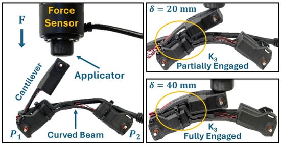
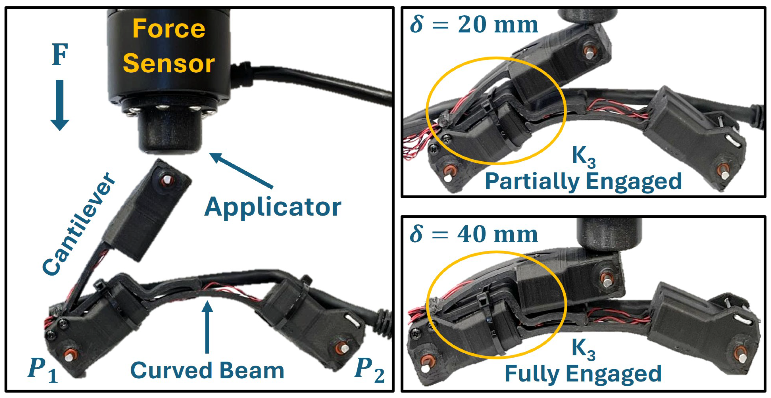
To validate our deflection and stiffness models described in Section 3, we mounted a 6-axis force/torque (FT) sensor (Rokubi Serial from Bota Systems, Zürich, CHE) (with a reported noise-free resolution of 0.15 N) in the collet of an end mill and used a manual lever to apply vertical compressive force to the robot with a cylindrical applicator (see Figure 11). Prior to collecting stiffness data, we cycled the prototype chassis through repeated compression/relaxation (via multiple pipe-entry cycles during development testing) so the measured stiffness corresponds to a repeatable post-break-in state of the chassis. After break-in, we compressed the robot until the lower flexure was nearly flat, and then removed the load completely and repeated the process for a total of five loading cycles.

Figure 11. Vertical force and displacement measurement test rig with a Rokubi force/torque sensor and digital caliper to measure position. Right: View of upper motor housing engaging curved spring (K₃) through adapter plate.

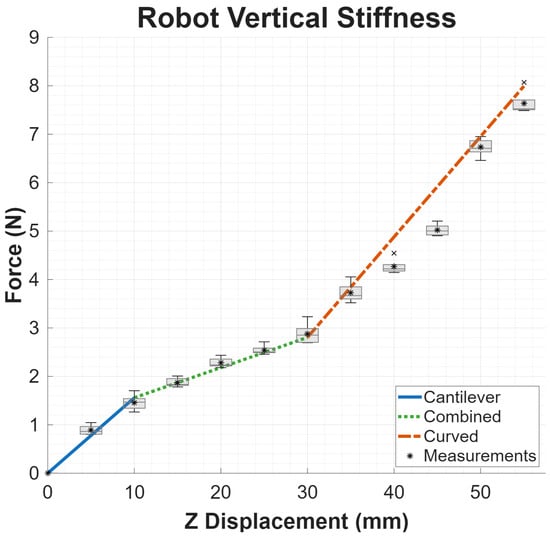
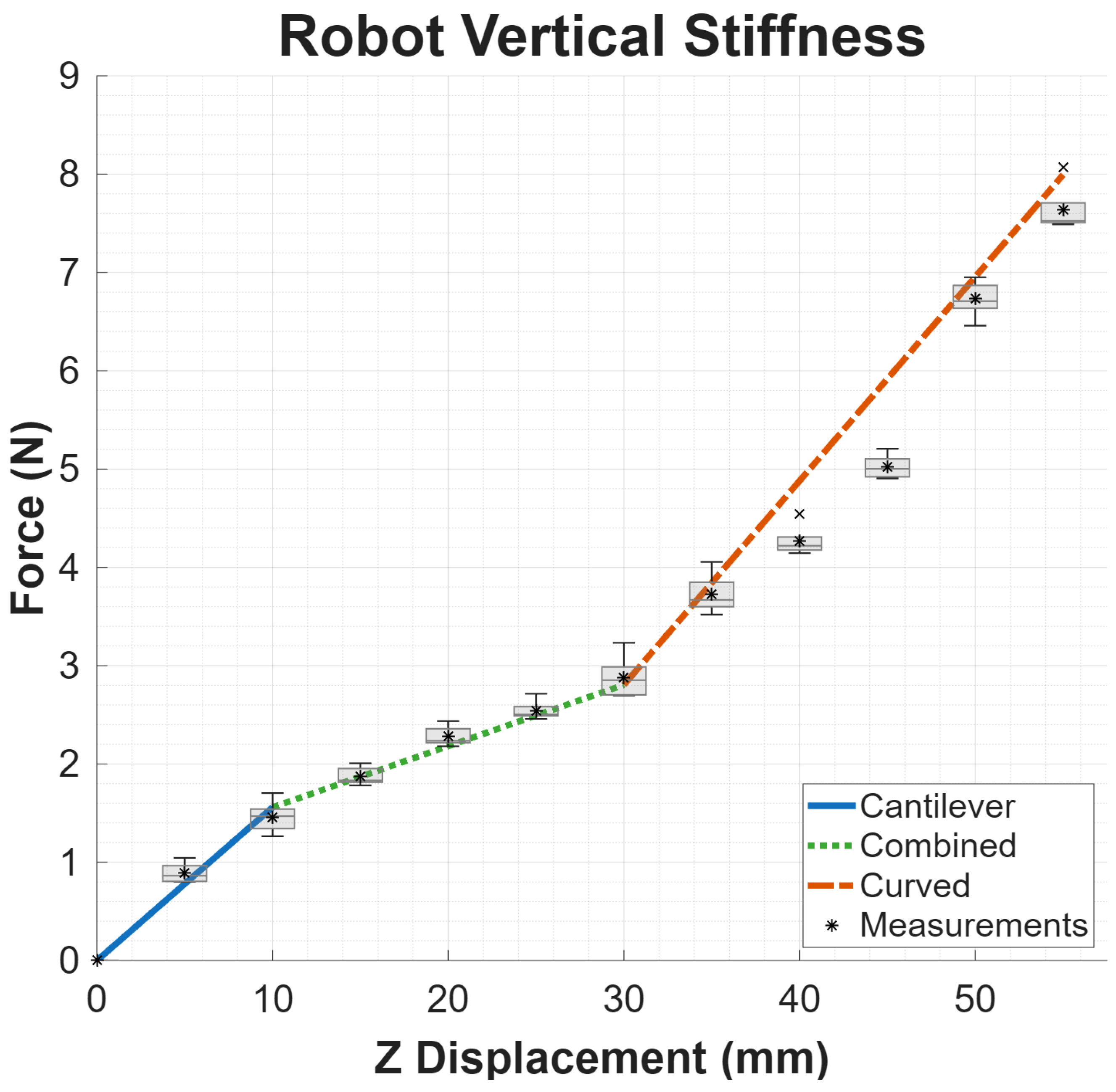
For each loading cycle, we measured reaction force versus imposed displacement at 11 discrete vertical points in 5 mm increments by averaging several seconds of FT data recorded at 100 Hz. Box plots showing the lower and upper quartiles, minimum/maximum, median (horizontal line) and mean (asterisk) of the measured force distributions at each location are shown in Figure 12, and Table 3 provides the numerical values.

Figure 12. Measured force vs. displacement across five loading cycles with vertical load applied to upper chassis. Modeled stiffness (solid and dashed lines) closely matches measured values (asterisks/box-and-whiskers) for each of the three stages of compression.

Table 3. Minimum, maximum, mean and standard deviation of forces measured at each stage of vertical displacement across five loading cycles.

Displacement (mm)	Min (N)	Max (N)	Mean (N)	$\mathit{\sigma }$ (N)
5	0.80	1.04	0.89	0.10
10	1.26	1.70	1.46	0.16
15	1.78	2.01	1.88	0.09
20	2.18	2.44	2.28	0.10
25	2.46	2.71	2.54	0.10
30	2.70	3.23	2.88	0.22
35	3.52	4.05	3.73	0.20
40	4.15	4.54	4.26	0.16
45	4.90	5.21	5.02	0.12
50	6.46	6.95	6.73	0.18
55	7.49	8.07	7.64	0.25

After measuring the reaction forces, we applied Equations (13) and (15) to compute $r_{eff}=52.94$ mm and $\beta =67.76$° and computed the estimated vertical reaction force at each displacement using Equations (9)–(12) (with flexural stiffness $E=3.0\times {10}^9$ Pa corresponding to the 3D-printed Onyx body material [35]). In this prototype, $\eta =0.5$ was selected as a first-order approximation of partial lower-flexure engagement during the transition region, corresponding to approximately half of the curved beam arc effectively contributing to vertical compliance. Figure 12 shows that the estimated forces (solid and dashed lines) closely match the measured values (asterisks/boxes). The coefficient of determination ($R^2$) and root-mean-square error (RMSE) for the estimated forces at each stage of compression compared to the mean measured values are listed in Table 4 below.

Table 4. Force estimation metrics compared to the mean measured value at each stage of vertical displacement.

Stage	Range (mm)	${\mathit{R}}^2$	RMSE (N)
Cantilever ($K_1$)	0–10	0.979	0.09
Combined ($K_2$)	10–30	0.992	0.07
Curved ($K_{3_{corr}}$)	30–55	0.969	0.48
Average	0–55	0.959	0.21

4.1.3. Manufacturing Variability: Dimensional Consistency

To assess the effect of manufacturing variability on the compliant printed components, we printed three nominally identical copies of the chassis components using the same material, printer settings, and build orientation as the tested prototype.

Dimensional consistency across prints was assessed by measuring representative width, length and thickness dimensions on each component and comparing each to the nominal/model value for that dimension. Table 5 shows the average error in printed component dimensions compared to the nominal value, along with the standard deviation across components, with W, L, and T representing width, length and thickness measurements, respectively.

Table 5. Dimensional variation across three sets of 3D-printed parts (measured vs. nominal). All values reported in millimeters.

Component	${\mathit{W}}_{\mathit{err}\mathbf{,}\mathit{avg}}$	${\mathit{L}}_{\mathit{err}\mathbf{,}\mathit{avg}}$	${\mathit{T}}_{\mathit{err}\mathbf{,}\mathit{avg}}$	${\mathit{\sigma }}_{{\mathit{W}}_{\mathit{err}}}$	${\mathit{\sigma }}_{{\mathit{L}}_{\mathit{err}}}$	${\mathit{\sigma }}_{{\mathit{T}}_{\mathit{err}}}$
Motor Housing	0.068	0.059	0.004	0.055	0.032	0.030
Upper Flexure	0.076	−0.068	0.123	0.036	0.114	0.016
Lower Flexure	0.030	0.024	0.119	0.006	0.024	0.063

For the curved lower flexure component, we also compared the radius of curvature of the printed components to the nominal value from the CAD model. To estimate the unloaded radius of curvature for the printed parts, we created orthogonal (side-view) images of the curves with 600 DPI flatbed scans. Points in the scanned images were selected along the outer edge of each curved member, converted from pixels to millimeters using the scan resolution, and fit to a circle using least squares. The fitted radius was used as the effective natural radius of curvature for each part, and part-to-part variability was quantified using the standard deviation and coefficient of variation compared to the nominal value. For the tested components, the nominal radius was 26.92 mm and the measured radii were 26.83 mm, 26.65 mm and 27.05 mm, with a mean RMSE of 0.03 mm for the fits, a mean measured radius of 26.84 mm, and a standard deviation of ${\sigma }_R=0.17$ mm, corresponding to a coefficient of variation of $C{V}_R=0.62$%.

The small variation in both the linear and curved dimensions in the printed geometry—with standard deviations less than 0.2 mm across all measurements—indicates good repeatability over the tested sample set.

4.1.4. Manufacturing Variability: Stiffness

In addition to geometric dimensions, we also measured stiffness as an indicator of variation in as-printed material properties. The effective stiffness of the upper flexure components was measured using a prescribed-deflection test. Each part was clamped in a vise at a fixed datum location on the part so the cantilever arm extended freely above a rigid metal platform which restricts maximum vertical deflection. The vertical distance between the top edge at the end of the cantilever arm and the surface of the rigid platform was set to 10 mm using a manual stage and measured with digital calipers. In this configuration, we used the Rokubi FT sensor with a cylindrical applicator noted above to deflect the free end of the cantilever until it contacted the platform. The force immediately prior to contact (visible as a distinct change/corner in the force vs. time curve) was used to estimate the effective stiffness as

$$K_{eff}={\displaystyle \frac{F_{pre-contact}}{{\delta }_{vertical}}}.$$

Each part was preconditioned with 10 or more loading/break-in cycles before data were recorded, after which we performed five deflection cycles with each part and computed the average ($K_{eff,avg}$), standard deviation (${\sigma }_{K_{eff}}$), and coefficient of variation ($C{V}_{K_{eff}}$) of the effective stiffness across parts. The results of these tests are reported in Table 6 below.

Table 6. Variation in effective stiffness across three sets of 3D-printed upper flexures.

Copy #	${\mathit{K}}_{\mathit{eff}\mathbf{,}\mathit{avg}}$ (N/m)	${\mathit{\sigma }}_{{\mathit{K}}_{\mathit{eff}}}$ (N/m)	${\mathit{CV}}_{{\mathit{K}}_{\mathit{eff}}}$ (%)
1	700.8	3.49	0.50
2	704.9	3.24	0.46
3	700.8	3.74	0.53
All	702.1	1.95	0.28

Although this sample size does not fully characterize production-scale variability or assembled-robot repeatability, the measured dimensional and stiffness variation was small relative to the model uncertainties considered here. The small part-to-part variation in effective stiffness shown in Table 6 suggests that geometric manufacturing variability is unlikely to dominate the first-order stiffness trends reported in this work.

4.2. Pull Force Estimation for Straight Pipe and Elbow

Using the pull-force estimation framework developed in Section 3.4, we estimated SPIINE’s available pull force in (i) a straight 53 mm ID pipe (see Figure 10a) and (ii) a tight 90° elbow (76 mm radius) under the minimum-compression condition (see Figure 10b).

4.2.1. Straight Pipe Estimate

For a 53 mm (2 in) ID pipe, the inner radius is $r=26.25$ mm. With track width $w_t=38.48$ mm, we computed the wheel contact angle (see Figure 10a) from Equation (17) as $\theta =42.9°$. Using Equation (16), the compressed robot height in straight pipe is $h_{c,s}=35.72$ mm, and with an uncompressed height $h_0=81.9$ mm, the deflection is ${\delta }_s=h_0-h_{c,s}=46.15$ mm. Using Equations (11) and (12) with $K_{3_{corr}}$, we find the corresponding vertical reaction force $F_v\left({\delta }_s\right)=6.16$ N. Projecting to normal force, $F_{n,s}=F_v\left({\delta }_s\right)sin\left(\theta \right)=4.19$ N. Finally, with $\mu \approx 2.1$ (see Section 2.3), we get

$$F_{pull,straight}\approx 17.59N.$$

4.2.2. Elbow Estimate

For the 90° elbow with a 76 mm radius, we estimate the minimum pull force case occurring in the 0° “natural” orientation (see Figure 6). Applying the geometric constraints shown in Figure 10b (including fixed effective arc length $s_{eff}=112.6$ mm), we obtain a compressed height in the elbow of $h_{c,e}=60.1$ mm, and thus ${\delta }_e=h_0-h_{c,e}=21.8$ mm. Using Equation (12) to compute the vertical reaction force at ${\delta }_e$ and then converting to pull force using the relationship outlined in Section 3.4 yields

$$F_{pull,elbow}\approx 6.55\mathrm{N}.$$

4.3. Hardware Prototype/System-Level Performance

We performed several hardware experiments in representative pipe setups to characterize the system-level performance of our compliant pipe inspection robot. Unless noted otherwise, all experiments used an 18 V benchtop supply (2.25 A limit; regulated by custom PCBs to 12 V for motors and 3–5 V for internal electronics) and a 33.5 m Cat6A tether for power and communications; ROS2 logging recorded IMU-based roll and motor currents.

4.3.1. Friction and Pull Force Measurements

To estimate available traction, we attached a single-axis force gauge to the SPIINE chassis with a nylon cord and pulled the unpowered robot through a straight segment of steel pipe. Force was applied gradually to observe the maximum limit achieved before breaking static friction and moving the vehicle. This passive test characterizes the wheel–pipe friction limit associated with the chassis normal force. Because we configured the motor torque limit (via hardware current limiting) to exceed the torque required to reach this friction limit, the passive traction measurement should provide an upper bound on the pull force that can be generated by the robot’s wheels.

To measure actuator-generated pull force, we attached the force gauge to the back of the robot and commanded the robot to drive forward in the pipe while the gauge was held in a fixed position. The gauge provided a resisting load while the robot’s motors actively drove the wheels against the pipe wall. The reported force corresponds to the maximum tensile load generated by the robot immediately before wheel slip or motor stall. In our experiments, we observed the largest measured loads when the motors reached the motor-driver current limit (which protects the gear train from damage). The peak actuator-generated pull force closely matched the peak friction resistance observed in the unpowered pull tests, within the sensor noise.

In straight pipe, the maximum force measured was ≈16.5 N (3.7 lb). This pull force is 8.4× the weight of the robot (1.96 N), and our estimated pull force of 17.59 N was within 6.9% of this measured value with an error of 1.13 N.

The measured pull force reduced to ≈7.56 N (1.70 lb) while the robot passed through a 90° elbow (radius: 76 mm, 3 in) in the 0° orientation shown in Figure 6. Our estimated minimum elbow pull force of 6.55 N is within 13.3% of the measured value with an error of 1.01 N. The notable increase in relative error for this estimate compared to the straight pipe configuration is likely due to the fact that the computed value for the compressed height in the elbow $h_{c,e}$ assumes the vehicle’s roll orientation is perfectly aligned with the elbow’s plane of curvature, but some misalignment and/or variation of roll angle during hardware experiments is likely. This variation in roll orientation would result in increased deflection/friction in hardware experiments, and thus a higher actual pull force (as was measured) compared to the idealized condition.

The prototype thus meets our conservative 12 N target in straight steel pipe but not in the minimum-compression 0° elbow configuration. This indicates that the present design provides sufficient overhead for the tested long-distance tether traversal but that future payload-towing applications requiring sustained high load through tight elbows may require increased chassis preload, higher-friction wheel materials, shorter towing distances, or active normal-force control, etc.

4.3.2. Bend Traversal at Various Orientations

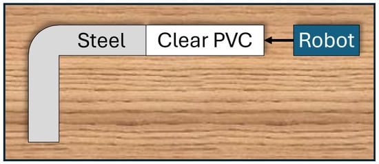
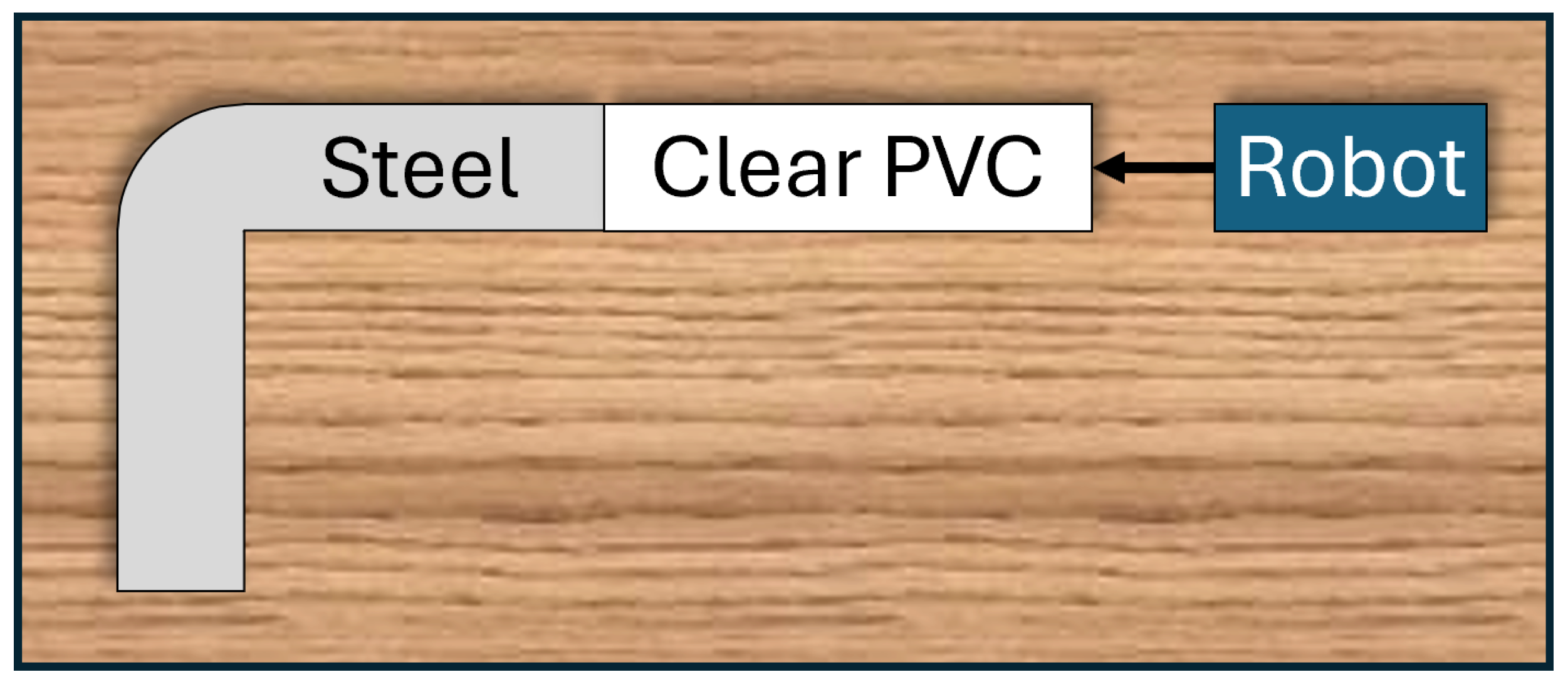
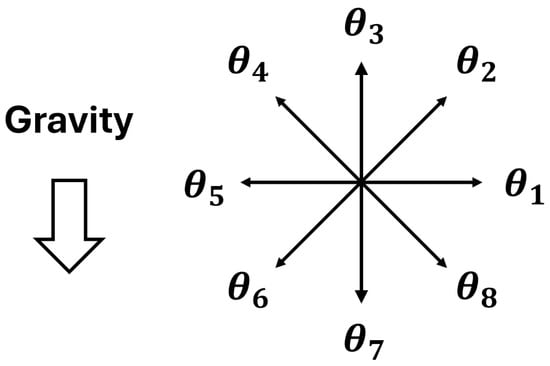
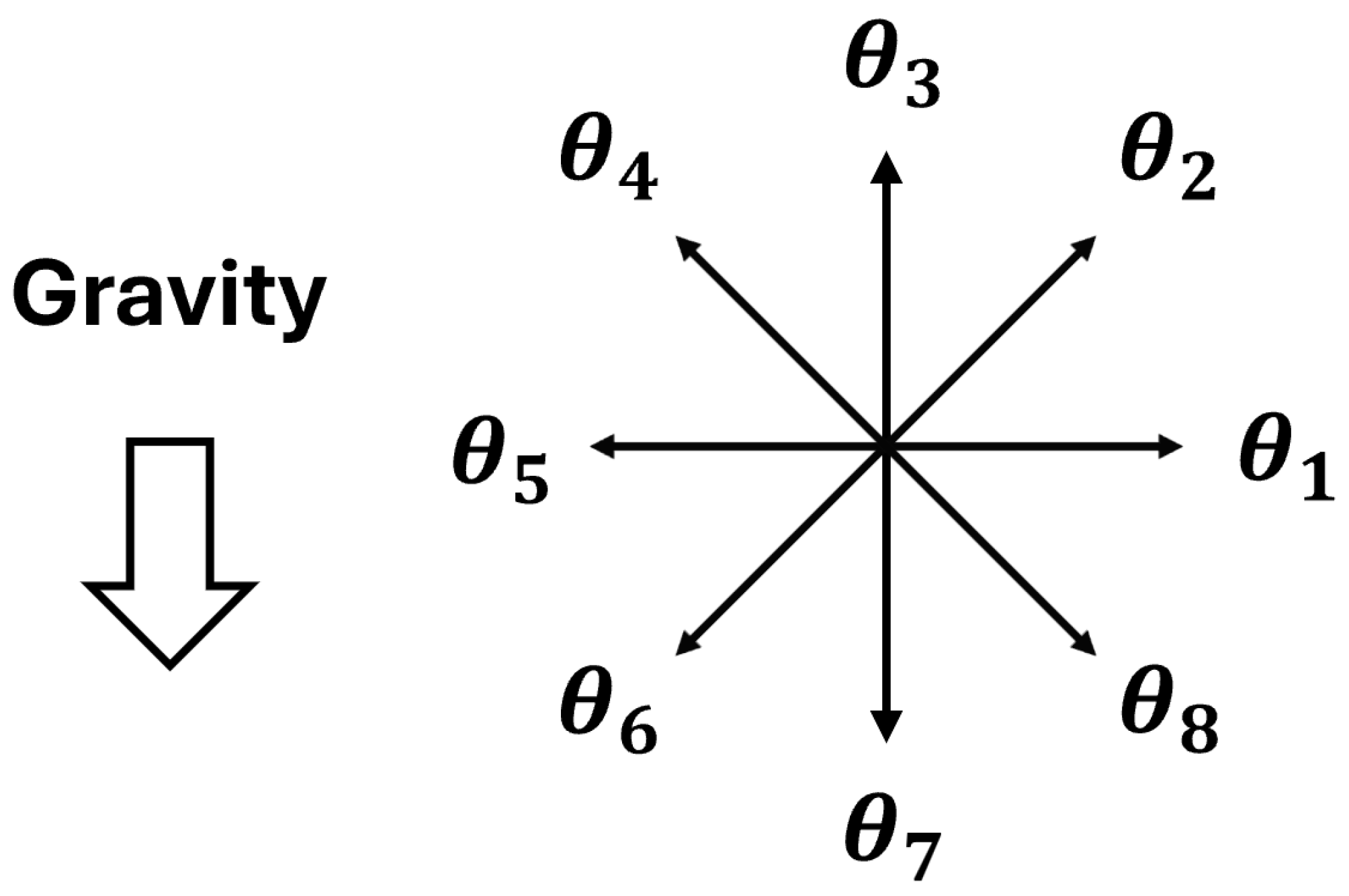
One key advantage of our compliant robot design is its ability to traverse tight bends at a variety of orientations spanning 360°, thus eliminating the need for active steering/orientation control. We verified this capability by driving the robot through a tight 90° elbow with a bend radius of 76 mm (3 in) on a tabletop setup, with eight different entry orientations (${\theta }_1-{\theta }_8$) in increments of 45° (rotated counter-clockwise about the robot’s forward axis), where ${\theta }_1$ corresponds to the 0° “natural” orientation (see Figure 6, Figure 13 and Figure 14).

Figure 13. Top view of tabletop setup to test traversal of tight 90° bends with various robot orientations relative to the bend curvature. Steel elbow bend radius: 76 mm.

Figure 14. Vehicle entry angles where each line/arrow represents the “up” direction of the robot (e.g., ${\theta }_1$ corresponds to the 0° “natural” orientation relative to the elbow as shown in Figure 6).

In each experiment, the robot entered the pipe, drove forward through the tight 90° bend with its “up” direction matching the corresponding pipe entry angle ${\theta }_n$, and then reversed back through the bend to return to the starting point. Across all starting orientations, the robot successfully traversed the elbow in forward and reverse, consuming ≈1.5–2 W of power through both the straight and curved portions of the pipe (see Table 7 for a summary of results). Some occasional individual motor stalls were observed while the robot was traversing the elbow, particularly in the ${\theta }_5$ orientation, where the elbow curvature is opposite (rotated 180°) to the robot’s “natural” curvature. However, these transient stalls resolved quickly and did not cause any noticeable disruption in robot motion around the bend.

Table 7. Results of SPIINE 90° elbow traversal at 8 entry orientations.

Entry Orientation	Forward Traversal	Reverse Traversal	Observed Stalls
${\theta }_1=0°$	Success	Success	None
${\theta }_2=45°$	Success	Success	None
${\theta }_3=90°$	Success	Success	None
${\theta }_4=135°$	Success	Success	None
${\theta }_5=180°$	Success	Success	Occasional, transient
${\theta }_6=225°$	Success	Success	None
${\theta }_7=270°$	Success	Success	None
${\theta }_8=315°$	Success	Success	None

4.4. Long-Distance Operation

To stress-test the electronics, data streaming, and motors/motor drivers, and test power delivery over a long distance, we successfully drove the robot downward into a 90° steel elbow, horizontally through 30 m (100 ft) of PVC pipe (10 × 10 ft segments joined with flexible couplers for long-run endurance testing), through a second 90° steel elbow, upward 46 cm, and then reversed back to the starting point (round-trip distance: ≈60 m). The average speed during this test was 0.77 m/min (2.54 ft/min) and average power consumption was 2 W during the straight section and ≈3.5 W during the vertical climb at the end. We also verified power delivery and video/telemetry streaming over a 110 m (350 ft) tether with a separate tether link integrity test.

4.5. Scope and Future Work

Pull-force tests were performed in steel pipe to match the intended inspection environment and friction characterization, whereas the 60 m endurance test used PVC pipe to provide a lightweight, rapidly reconfigurable long-run testbed. Because pipe material affects wheel friction and power consumption, the PVC test should be interpreted as a system-level endurance and communications demonstration rather than a direct validation of steel-pipe traction performance over 60 m.

The experiments reported here were conducted primarily on a single hardware prototype and are intended to validate the feasibility of the design and the accuracy of the first-order stiffness model rather than to characterize manufacturing variability across multiple units. The reported long-distance and tether tests demonstrate successful operation in representative configurations, but future work should include repeated trials across multiple printed chassis, pipe materials, and contamination conditions to quantify robustness, variation in wheel friction, and changes in performance after extended wear.

5. Conclusions

In this work, we presented SPIINE, a compliant six-wheeled robot that addresses the significant challenges imposed by size constraints, tight bends, and long pipe lengths to enable internal inspection of small pipes. SPIINE can traverse 53 mm (2 in) ID pipes with tight 90° elbows (radius as small as 76 mm (3 in)), transmit power and data (including high-resolution video) over long tethers (verified to 110 m), and generate up to 16.5 N of pull force in straight steel pipe—over eight times the weight of the robot—to support towing of NDT sensor payloads.

Experiments with a hardware prototype demonstrated that our analytical models for estimating robot stiffness and normal force generation capability closely match the real system—estimating chassis vertical reaction force within 0.21 N RMSE, and pull force within 7–13% for two tested operating conditions. We also demonstrated that the robot can traverse a tight 90° elbow in forward and reverse at eight tested entry roll orientations spanning 360°, and consumes only ≈2 to 3.5 W across representative test segments.

Beyond validating the specific SPIINE prototype, the stiffness-to-pull-force modeling approach provides a useful framework for designing flexible-bodied pipe-traversing robots under coupled diameter, bend-radius, traction, and payload constraints. While the model is intentionally first-order and should be recalibrated for different materials, wheel geometries, and pipe conditions, it offers a practical means of linking body compliance to available tractive force during early-stage robot design.

In future work, we plan to test integration with an NDT sensor payload to enhance visual inspections and possibly integrate additional sensors and algorithms to enable mapping of pipe geometry. We will also investigate methods for controlling the orientation of the camera, limiting vehicle roll during forward motion, and optimizing component geometry to incorporate all of the sensing and control electronics into the drive body for a more compact overall footprint.

References

- Arifin, M.D.; Dariansyah, M.R. Lifespan Estimation of Galvanized Steel and Stainless Steel Pipe. Int. J. Mar. Eng. Innov. Res. 2023, 8, 468–476. Available online: https://iptek.its.ac.id/index.php/ijmeir/article/view/18650/pdf_180 (accessed on 23 September 2026). [CrossRef] [Scilit]
- Wang, Y.; Song, F.; Feng, Q.; Qiao, W.; Dong, S.; Jiang, Y.; Ma, Q. Basic Theory and Applications of Oil and Gas Pipeline Non-Destructive Testing Methods. Energies 2024, 17, 6366. [Google Scholar] [CrossRef] [Scilit]
- Dwivedi, S.K.; Vishwakarma, M.; Soni, P. Advances and Researches on Non Destructive Testing: A Review. Mater. Today Proc. 2018, 5, 3690–3698. [Google Scholar] [CrossRef] [Scilit]
- Ma, Q.; Liang, W.; Zhou, P. A Review on Pipeline In-Line Inspection Technologies. Sensors 2025, 25, 4873. [Google Scholar] [CrossRef] [Scilit] [PubMed]
- Kahnamouei, J.T.; Moallem, M. A comprehensive review of in-pipe robots. Ocean. Eng. 2023, 277, 114260. [Google Scholar] [CrossRef] [Scilit]
- Elankavi, R.S.; Dinakaran, D.; Chetty, K.; Ramya, M.M.; Samuel, H. A Review on Wheeled Type In-Pipe Inspection Robot. Int. J. Mech. Eng. Robot. Res. 2022, 11, 745–754. [Google Scholar] [CrossRef] [Scilit]
- Verma, A.; Kaiwart, A.; Dubey, N.D.; Naseer, F.; Pradhan, S. A review on various types of in-pipe inspection robot. Mater. Today Proc. 2022, 50, 1425–1434. [Google Scholar] [CrossRef] [Scilit]
- Kazeminasab, S.; Sadeghi, N.; Janfaza, V.; Razavi, M.; Ziyadidegan, S.; Banks, M.K. Localization, Mapping, Navigation, and Inspection Methods in In-Pipe Robots: A Review. IEEE Access 2021, 9, 162035–162058. [Google Scholar] [CrossRef] [Scilit]
- Ismail, I.N.; Anuar, A.; Sahari, K.S.M.; Baharuddin, M.Z.; Fairuz, M.; Jalal, A.; Saad, J.M. Development of in-pipe inspection robot: A review. In Proceedings of the 2012 IEEE Conference on Sustainable Utilization and Development in Engineering and Technology (STUDENT), Kuala Lumpur, Malaysia, 6–9 October 2012; pp. 310–315. [Google Scholar] [CrossRef] [Scilit]
- Jang, H.; Kim, T.Y.; Lee, Y.C.; Song, Y.H.; Choi, H.R. Autonomous Navigation of In-Pipe Inspection Robot Using Contact Sensor Modules. IEEE/ASME Trans. Mechatron. 2022, 27, 4665–4674. [Google Scholar] [CrossRef] [Scilit]
- Rusu, C.; Tatar, M.O. Adapting Mechanisms for In-Pipe Inspection Robots: A Review. Appl. Sci. 2022, 12, 6191. [Google Scholar] [CrossRef] [Scilit]
- Nguyen, T.P.; Nguyen, H.; Minh Ngo, N.; Ngo, H.Q.T. Experimental Verification of the Field Robotic System for Pipeline Maintenance. IEEE Access 2025, 13, 13782–13795. [Google Scholar] [CrossRef] [Scilit]
- Venkateswaran, S.; Chablat, D. A New Inspection Robot for Pipelines with Bends and Junctions. In Advances in Mechanism and Machine Science; Mechanisms and Machine Science; Uhl, T., Ed.; Springer: Cham, Switzerland, 2019; Volume 73, pp. 33–42. HAL: hal-02098350. [Google Scholar] [CrossRef] [Scilit]
- Kusunose, K.; Akagi, T.; Dohta, S.; Kobayashi, W.; Nakagawa, K. Development of Pipe Holding Mechanism and Bending Unit Using Extension Type Flexible Actuator for Flexible Pipe Inspection Robot. Int. J. Mech. Eng. Robot. Res. 2019, 8, 129–134. [Google Scholar] [CrossRef] [Scilit]
- Kakogawa, A.; Ma, S. A Multi-link In-pipe Inspection Robot Composed of Active and Passive Compliant Joints. In Proceedings of the 2020 IEEE/RSJ International Conference on Intelligent Robots and Systems (IROS), Las Vegas, NV, USA, 24 October 2020–24 January 2021; pp. 6472–6478. [Google Scholar] [CrossRef] [Scilit]
- Dertien, E.; Stramigioli, S.; Pulles, K. Development of an inspection robot for small diameter gas distribution mains. In Proceedings of the 2011 IEEE International Conference on Robotics and Automation (ICRA), Shanghai, China, 9–13 May 2011; pp. 5044–5049. [Google Scholar] [CrossRef] [Scilit]
- Sugizaki, Y.; Kakogawa, A. A V-shaped In-pipe Robot Capable of Drawing Route Maps for Both 3-in and 4-in Diameters using Only Low-cost Internal Sensors. In Proceedings of the 2025 IEEE/RSJ International Conference on Intelligent Robots and Systems (IROS), Hangzhou, China, 19–25 October 2025; pp. 17580–17585. [Google Scholar] [CrossRef] [Scilit]
- Kakogawa, A.; Hirose, C.; Ma, S. A Standards-based Pipeline Route Drawing System using a Towed Sensing Unit. In Proceedings of the 2022 IEEE/RSJ International Conference on Intelligent Robots and Systems (IROS), Kyoto, Japan, 23–27 October 2022; pp. 7167–7173. [Google Scholar] [CrossRef] [Scilit]
- Suzumori, K.; Miyagawa, T.; Kimura, M.; Hasegawa, Y. Micro inspection robot for 1-in pipes. IEEE/ASME Trans. Mechatron. 1999, 4, 286–292. [Google Scholar] [CrossRef]
- SeeSnake® MicroREEL CA-350 Video Inspection System|RIDGID Tools. Available online: https://www.ridgid.com/us/en/seesnake-microreel-ca350-inspection-system (accessed on 26 September 2026).
- Spectis Robotics. CRXS-50 Pipe Crawler. Available online: https://spectisrobotics.com/products/crxs-50-pipe-crawler/ (accessed on 8 October 2026).
- VersaTrax™ ISeries Inspection Crawlers|Eddyfi. Available online: https://robotics.eddyfi.com/versatrax-i-series (accessed on 26 September 2026).
- Kamezaki, M.; Yamaguchi, K.; Zhao, W.; Yoshida, K.; Koike, T.; Miyake, S.; Sugano, S. SPIRA: Small Gas Pipeline Inspection Robot with Spiral Leg-Wheel Mechanism and Single Bending Joint. IEEE Robot. Autom. Lett. 2025, 10, 12676–12683. [Google Scholar] [CrossRef] [Scilit]
- Nguyen, T.L.; Blight, A.; Pickering, A.; Jackson-Mills, G.; Barber, A.R.; Boyle, J.H.; Richardson, R.; Dogar, M.; Cohen, N. Autonomous control for miniaturized mobile robots in unknown pipe networks. Front. Robot. AI 2022, 9, 997415. [Google Scholar] [CrossRef] [Scilit] [PubMed]
- Roh, S.g.; Choi, H.R. Differential-drive in-pipe robot for moving inside urban gas pipelines. IEEE Trans. Robot. 2005, 21, 1–17. [Google Scholar] [CrossRef] [Scilit]
- Kakogawa, A.; Murata, K.; Ma, S. Automatic T-Branch Travel of an Articulated Wheeled In-Pipe Inspection Robot Using Joint Angle Response to Environmental Changes. IEEE Trans. Ind. Electron. 2023, 70, 7041–7050. [Google Scholar] [CrossRef] [Scilit]
- Heinrich, G.; Klüppel, M. Rubber friction, tread deformation and tire traction. Wear 2008, 265, 1052–1060. [Google Scholar] [CrossRef] [Scilit]
- Gabriel, P.; Thomas, A.G.; Busfield, J.J.C. Influence of interface geometry on rubber friction. Wear 2010, 268, 747–750. [Google Scholar] [CrossRef] [Scilit]
- Macenski, S.; Foote, T.; Gerkey, B.; Lalancette, C.; Woodall, W. Robot Operating System 2: Design, architecture, and uses in the wild. Sci. Robot. 2022, 7, eabm6074. [Google Scholar] [CrossRef] [Scilit] [PubMed]
- Bradski, G. The OpenCV Library. Dr. Dobb’s J. Softw. Tools 2000. [Google Scholar] [CrossRef] [Scilit]
- Pytel, A.; Kiusalaas, J. Mechanics of Materials, 2nd ed.; Cengage Learning: Stamford, CT, USA, 2012; pp. 428–429. [Google Scholar]
- Budynas, R.G.; Nisbett, J.K. Shigley’s Mechanical Engineering Design, 9th ed.; McGraw-Hill: New York, NY, USA, 2011; pp. 164–171. [Google Scholar]
- Bulwahn, L. Intersecting Chords Theorem. Archive of Formal Proofs. Formal Proof Development. 2016. Available online: https://isa-afp.org/entries/Chord_Segments.html (accessed on 19 August 2026).
- Beléndez, T.; Neipp, C.; Beléndez, A. Large and small deflections of a cantilever beam. Eur. J. Phys. 2002, 23, 371–379. [Google Scholar] [CrossRef] [Scilit]
- Markforged. Onyx Material Specifications. 2026. Available online: https://support.markforged.com/portal/s/article/Onyx#specs (accessed on 19 August 2026).
Disclaimer/Publisher’s Note: The statements, opinions and data contained in all publications are solely those of the individual author(s) and contributor(s) and not of MDPI and/or the editor(s). MDPI and/or the editor(s) disclaim responsibility for any injury to people or property resulting from any ideas, methods, instructions or products referred to in the content. |
© 2026 by the authors. Licensee MDPI, Basel, Switzerland. This article is an open access article distributed under the terms and conditions of the Creative Commons Attribution (CC BY) license.