


Abstract
Precision agriculture requires robotic platforms capable of covering large cultivation areas while providing accurate positioning for localized crop monitoring and management operations. Cable-driven parallel robots (CDPRs) offer large workspaces and lightweight moving structures; however, their usable workspace is constrained by cable tension requirements. This study presents the experimental validation of AgroCableBot, a reconfigurable CDPR for precision agriculture previously proposed by the authors, in which the proximal cable attachment points are vertically reconfigured to increase the wrench-feasible workspace (WFW). Previous simulation results showed that this reconfiguration increases the WFW from approximately 58% to 100% of the geometrically admissible workspace for a minimum cable tension of 5 N. In this work, a physical prototype with adjustable anchor height was built, and a vision-based sensing system was integrated for end-effector localization, automatic calibration, and closed-loop trajectory tracking. Experimental validation included square and circular trajectories and an agricultural inspection trajectory over a seedling tray, executed at three anchor heights (400, 600 and 900 mm). The system achieved a three-dimensional RMSE between 1.9 and 2.6 mm, a 95th-percentile error below 4.5 mm, and a maximum tracking error of 6.0 mm, measured with the vision system. These results demonstrate the potential of AgroCableBot as a reconfigurable robotic platform for accurate crop monitoring and localized agricultural operations in protected cultivation environments.
1. Introduction
Cable-driven parallel robots (CDPRs) represent a distinctive class within modern robotics. In these systems, cables replace the traditional rigid links that connect the end-effector to the fixed structure, significantly reducing system inertia and enabling high speeds and accelerations with lower power requirements [1]. From a kinematic perspective, CDPRs provide accurate position and orientation control through cable length variation, offering remarkable flexibility and adaptability [2]. Owing to these characteristics, they have been successfully implemented in a wide range of applications, including physical rehabilitation [3,4,5,6,7,8,9], industrial manipulation, and structural inspection [10,11,12,13], where their low weight and high payload-to-power ratio provide significant advantages.
Over the last decade, CDPRs have experienced sustained growth across multiple application domains, ranging from manufacturing and construction [14,15,16,17] to wind tunnel instrumentation [18,19,20], inventory and industrial handling [21,22], and aerospace systems [23,24]. In the agricultural sector, platforms such as the ETH Field Phenotyping Platform (FIP) [25] and the NU-Spidercam system [26] have enabled the automation of large-scale agronomic data acquisition. Other developments, such as those proposed by [27,28], have explored cable-driven robotic configurations for harvesting and tropical fruit manipulation tasks. However, these agricultural platforms use fixed anchor points, and the trade-off between workspace and cable tension has not been studied for compact systems in protected cultivation. Consequently, CDPRs have attracted increasing interest in applications requiring high payload-to-weight ratios, large workspaces, and dynamic operation.
Despite these advances, CDPRs still face critical limitations that restrict their deployment in agricultural environments. The most significant challenges include: (i) a limited workspace, constrained by the need to maintain positive tension in all cables to prevent undesired oscillations, and (ii) low structural stiffness, which can reduce positioning accuracy during high-speed motions or under varying payload conditions [29,30,31]. These limitations hinder the adoption of CDPRs in agricultural tasks requiring accurate and repeatable positioning over large workspaces.
A reconfigurable CDPR can change the position of its cable anchor points to adapt the workspace, stiffness or cable tensions to the task [32,33]. This change can be discrete, when the anchor points are moved between tasks with the robot stopped, or continuous, when they move during operation. Other ways to enlarge the workspace include passive carriages, single cable loops, variable radius pulleys and additional cables [34]. In AgroCableBot, the four proximal anchor points are moved together along the vertical axis and fixed before each task. When the anchor points are lowered, the cables become closer to horizontal, and the cable tensions needed to support the end-effector weight increase. This keeps all cables in tension over a larger region and increases the WFW [34].
To overcome these limitations, this work presents the experimental validation of a reconfigurable cable-driven parallel robot architecture named AgroCableBot, specifically designed for the automation of greenhouse agricultural processes. The system constitutes the experimental extension of the theoretical framework previously introduced by the authors in [34], where the kinematic and structural foundations of the reconfigurable design were established. AgroCableBot incorporates an additional degree-of-freedom (DOF) along the z-axis, enabling the vertical adjustment of the cable anchoring points and operation under higher cable tensions. In the current prototype, this height is adjusted manually before each task. This reconfiguration increases the effective stiffness of the system and expands the Wrench-Feasible Workspace (WFW) from approximately 58% to 100% of the geometrically admissible workspace for N, as shown in simulation in [34]. Furthermore, the system integrates a vision-based sensing framework for automatic calibration, end-effector position estimation, and closed-loop trajectory control. This work extends the previous theoretical contribution through the experimental implementation and validation of the reconfigurable architecture, including the integration of vision-based sensing and feedback control, and the quantitative evaluation of end-effector positioning accuracy under representative geometric and agricultural trajectories.
The main objective of this work is to perform a comprehensive experimental validation of AgroCableBot by evaluating its positioning accuracy, stability, and control performance under different operating configurations. A key aspect of the proposed system is the integration of a vision-based sensing architecture for real-time end-effector localization, initial calibration, and closed-loop trajectory tracking. The sensing system provides continuous positional measurements that are integrated into the control loop to estimate the end-effector pose and evaluate trajectory-tracking performance. The obtained results establish a link between the theoretical design and its practical implementation, demonstrating the feasibility of the proposed sensor-integrated robotic architecture for precision agriculture and its potential for accurate agricultural operations in protected cultivation environments.
The previous work [34] presented the design of AgroCableBot and evaluated it only in simulation. In this work, the robot was built and tested experimentally. The main contributions are the following. First, the physical prototype was implemented with an adjustable anchor height. Second, a vision system was integrated, with an eye-to-hand camera for automatic calibration and closed-loop localization of the end-effector, and an eye-in-hand camera for crop images. Third, trajectory tracking was evaluated at three anchor heights ( = 400, 600 and 900 mm), with geometric trajectories and a crop inspection trajectory. Fourth, the tracking error was analyzed along each trajectory to identify where it increases and its main sources.
The remainder of this paper is organized as follows. Section 2 describes the design of AgroCableBot, including its mechanical, actuation, and vision subsystems. Section 3 presents the kinematic model, the position estimation with the vision system, and the control architecture. Section 4 reports the experimental results. Section 5 presents the discussion. Finally, Section 6 summarizes the main conclusions and outlines future research directions.
2. System Design of AgroCableBot
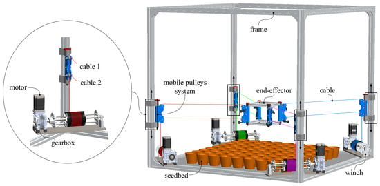
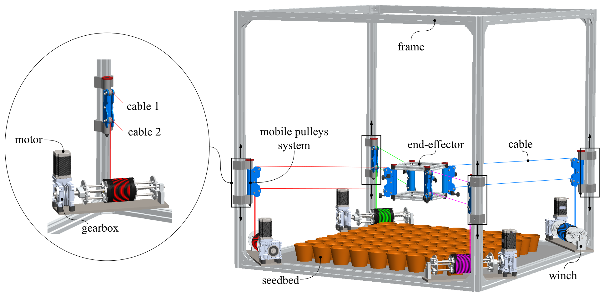
The design of AgroCableBot integrates mechanical, electronic, and computational systems to address common limitations of cable-driven parallel robots (CDPRs), including restricted workspace, reduced stability under load, and limited adaptability in dynamic environments, as illustrated in Figure 1. The system was specifically developed for agricultural applications, enabling high-precision and adaptable operations such as crop monitoring, irrigation, and seeding. AgroCableBot consists of five main subsystems: a fixed frame, a cable winch system, a pulley system, an end-effector, and a vision and inertial measurement system. The most relevant components and their functions within the overall system are described in the following subsections.
Figure 1.
CAD model of AgroCableBot, showing the fixed frame, four cable winch systems, double-pulley mechanisms that provide vertical reconfiguration of the cable anchor points, the end-effector, and eight cables arranged in four pairs.
The configuration of AgroCableBot corresponds to a suspended Cable-Driven Parallel Robot (CDPR), in which the end-effector is driven by four winches, each one moving a pair of parallel cables, and gravity keeps all cables in tension. The system provides five degrees-of-freedom: three translational motions along the Cartesian axes (x, y, z), one rotational motion about the z-axis, and an additional degree-of-freedom corresponding to the vertical displacement of the cable anchoring points on the frame. This vertical displacement is adjusted manually before each task and remains fixed during operation. This additional capability enhances the robot’s ability to operate in dynamic environments and perform complex agricultural tasks. The geometrically admissible workspace of the end-effector, limited by the frame, the pulley systems and the end-effector dimensions, is 800 × 800 mm in the -plane and 900 mm along the z-axis. This volume is taken as the 100% reference for the workspace percentages reported in this work. To ensure optimal performance, detailed technical specifications were established and are summarized in Table 1. These specifications include the main components, actuators, sensors, and transmission mechanisms, which were selected to provide the stability, accuracy, and adaptability required for operation in variable agricultural environments. Figure 1 presents the CAD model of AgroCableBot, highlighting the integration of its main subsystems, including the fixed frame, cable winch systems, double-pulley mechanisms, end-effector, and cable arrangement.
Table 1.
Specifications of the AgroCableBot robot.
2.1. Pulley System Design and Cable Arrangement
The pulley system of AgroCableBot was designed to maximize the stability and positioning accuracy of the end-effector by forming a cable parallelogram between each pair of pulleys. This geometric configuration ensures a uniform distribution of cable tensions and precise motion synchronization between the cable pairs located on the frame and those attached to the end-effector.
Each pulley simultaneously guides two cables from the winch systems to the end-effector, maintaining structural symmetry and ensuring coordinated control, as illustrated in Figure 1. In addition, the system incorporates an adjustable vertical anchoring mechanism that allows the pulleys to be displaced along the z-axis. This dynamic adjustment enlarges the workspace and enhances its adaptability to different crop heights and cultivation configurations. The end-effector is equipped with guitar tuning pegs coupled to an irreversible worm-gear mechanism, enabling cable tension adjustment during the initial calibration process while maintaining the robot’s operational accuracy throughout operation.
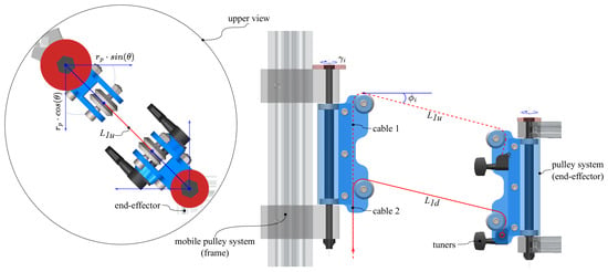
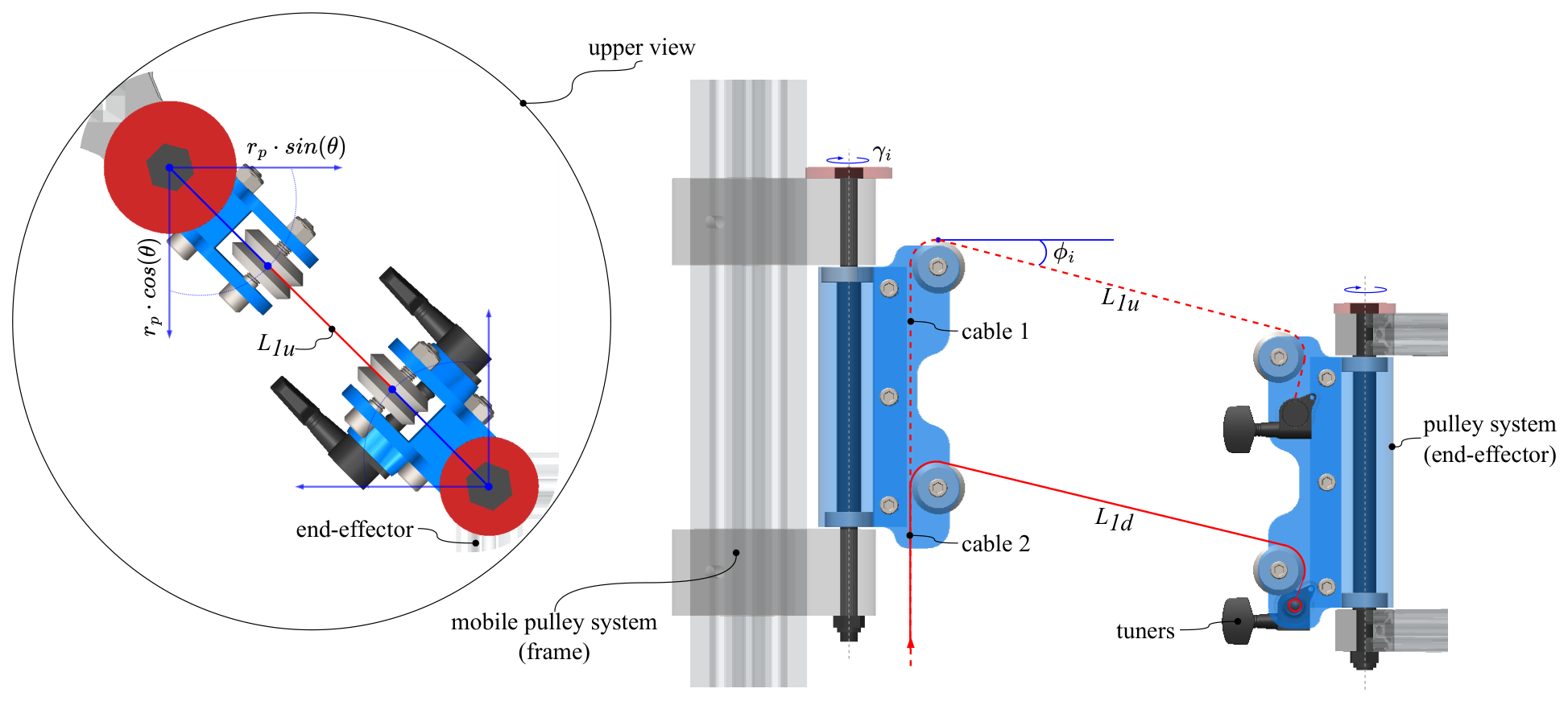
Figure 2 illustrates the pulley system, the additional degree-of-freedom along the z-axis, and the geometric correction applied to the cable length calculation by considering the angle formed with the pulley rotation axis. The complexity of this design arises from the fact that the cable attachment points do not remain fixed during motion but instead follow arc-shaped trajectories determined by the pulley rotation axis. Consequently, the control model incorporates dynamic variables that account for parameters such as the pulley radius (), the rotation angle (), and the dimensions of both the frame and the end-effector, as detailed in the previous study (see [34]). This approach provides a more flexible, stable, and adaptable robotic system capable of operating under a wide range of agricultural conditions.
Figure 2.
AgroCableBot pulley system. Side view of the mechanism incorporating the additional degree-of-freedom along the z-axis. The enlarged detail presents the top view used to geometrically correct the cable length calculation by accounting for the pulley system rotation angle.
2.2. Cable Winch System
The AgroCableBot cable winch system was designed to ensure stable, accurate, and reliable control of the cables driving the end-effector. Each module employs a motor with a nominal torque of 3 Nm, coupled to a worm-gear reducer with a 10:1 transmission ratio. This mechanism provides a self-locking effect that prevents unwanted end-effector displacements even when the motors are de-energized, which is essential for maintaining stability while handling variable payloads.
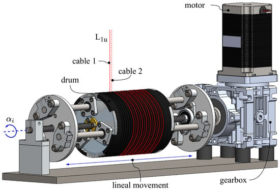
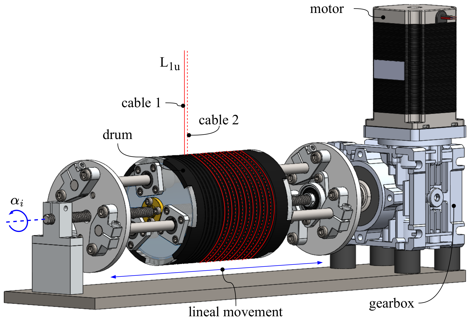
Each winch drum is manufactured with two parallel grooves that allow two cables to be wound or unwound simultaneously without overlap, ensuring uniform tension distribution. The drum, with a diameter of 88.4 mm, translates horizontally along an 8 mm lead trapezoidal screw and has a maximum travel of 140 mm, as shown in Figure 3. This design maintains a constant effective drum diameter regardless of the amount of stored cable, thereby ensuring a linear and accurate relationship between motor rotation and cable length variation during operation.
Figure 3.
AgroCableBot cable winch system. The assembly consists of a motor, a worm-gear reducer, a linear guide with a trapezoidal lead screw, and a dual-groove drum designed to wind two cables without overlap.
The selected cable material is ultra-high-molecular-weight polyethylene (UHMWPE) fiber, commercially known as Dyneema. This material was chosen over steel cables because of its excellent strength-to-weight ratio, high resistance to wear and fatigue, and superior flexibility. The cables have a breaking strength of 1108 N, and a minimum tension of N was used in the workspace analysis [34]. The weight of the end-effector (3 kg, 29.4 N) is supported by the vertical components of the cable tensions, as described by the static equilibrium in Section 3.1. The weight of the cables can be neglected: with a linear mass of about 0.3 g/m, the cable sag is about 0.1 mm at N and much smaller at the operating tensions. The cable elongation changes with the tension along the trajectory and is one of the error sources discussed in Section 5.
Overall, the winch system provides efficient and robust cable management, ensuring smooth force transmission and consistent end-effector positioning accuracy throughout the AgroCableBot workspace.
2.3. Vision-Based Sensing System
The AgroCableBot vision-based sensing system is designed to provide real-time localization of the end-effector, support the initial calibration procedure, and provide continuous feedback for trajectory tracking. During the initial calibration, a reference or home position is established through the detection of reference markers strategically placed on the robot frame and the end-effector. This procedure provides a consistent spatial reference for the position control and trajectory tracking algorithms.
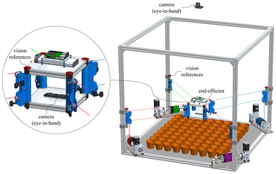
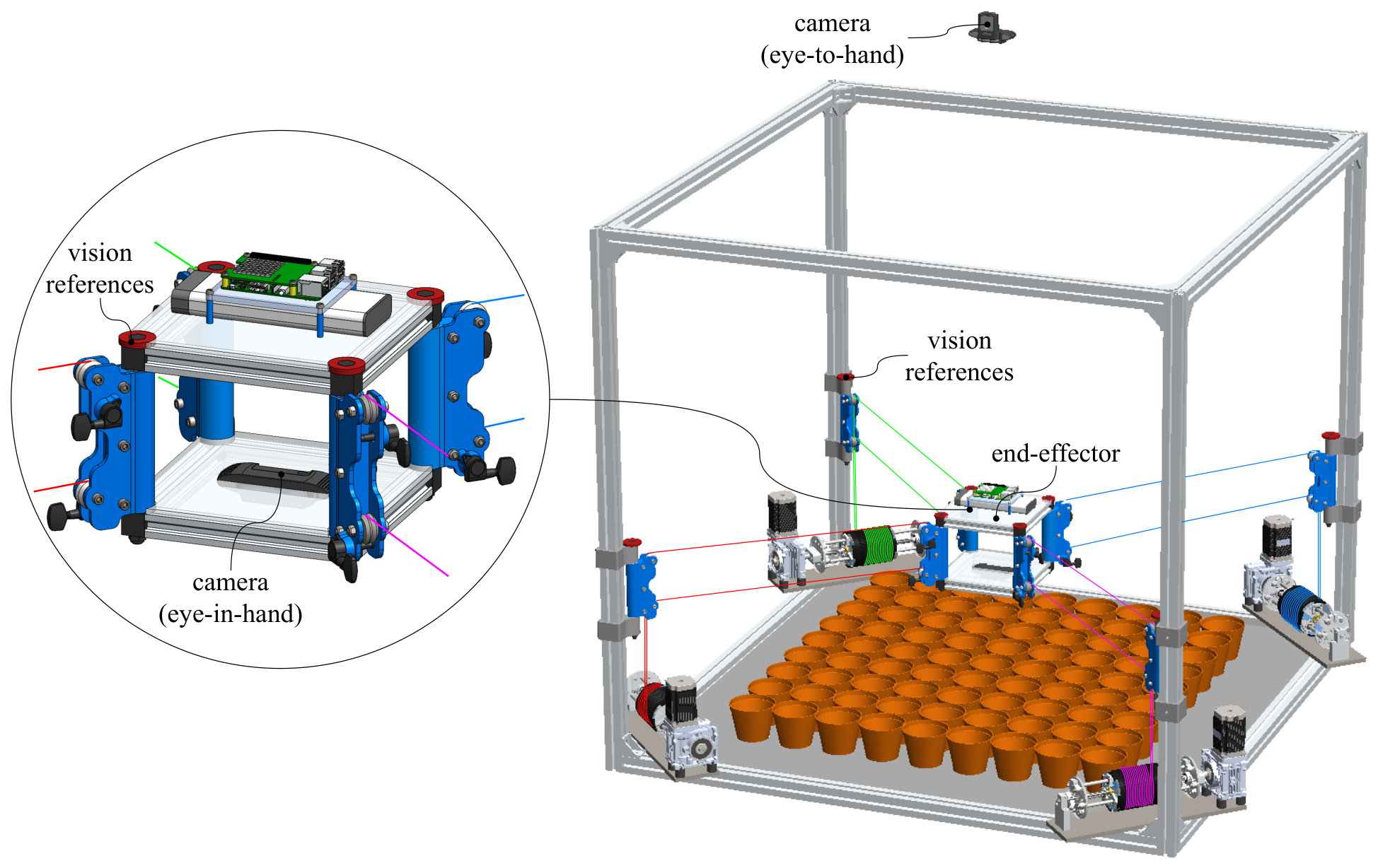
The system consists of two computer vision cameras operating cooperatively: an eye-in-hand (EIH) camera mounted directly on the end-effector and an eye-to-hand (ETH) camera installed on a support above the robot frame, at a height of 2270 mm above the floor, as illustrated in Figure 4. The EIH camera acquires images of the plants for crop monitoring from the end-effector, whereas the ETH camera provides a global view of the robot and its workspace and is used for calibration and localization. The ETH camera detects eight reference markers, four located at the pulley rotation axes of the frame and four on the end-effector, enabling the localization of the end-effector within the robot workspace (see [35] for further details). During operation, visual servoing techniques are employed to correct, in real time, the deviations between the desired and estimated end-effector positions, following the approach described by [36].
Figure 4.
AgroCableBot vision-based sensing system. The system consists of an eye-in-hand (EIH) camera mounted on the end-effector for crop imaging, an eye-to-hand (ETH) camera installed on a support above the robot frame, at a height of 2270 mm above the floor, for calibration and end-effector localization, eight red reference markers (four at the pulley rotation axes of the frame and four on the end-effector), and an inertial measurement unit (IMU) mounted on the end-effector.
The ETH camera plays a central role in the experimental sensing architecture. Its global view enables the detection of the reference markers on the robot frame, the definition of the workspace coordinate system, and the estimation of the end-effector position. A perspective transformation, computed from the four frame markers, is subsequently applied to compensate for perspective effects and establish the correspondence between image coordinates and physical coordinates in the -plane. The depth coordinate is estimated from the geometric relationship between the reference markers and the end-effector, using a height reference obtained with a calibration board placed at a known height, allowing the three-dimensional position of the end-effector to be obtained from the visual measurements.
During operation, the estimated end-effector position is continuously compared with the desired Cartesian trajectory. The resulting position error is provided as feedback to the control system, enabling real-time monitoring of the trajectory and correction of deviations through the inverse-kinematics and PID control architecture. This sensing-based feedback loop allows the robot to operate using the measured end-effector position rather than relying exclusively on the nominal position obtained from the actuator commands.
The integrated vision-based sensing system therefore provides the measurement layer required for end-effector localization, calibration, trajectory monitoring, and closed-loop control. This architecture establishes a direct connection between the sensing subsystem and the experimental evaluation of positioning accuracy presented in Section 4.
3. Mathematical Model, Sensing and Control System
This section presents the mathematical model, sensing architecture, and control system developed for the First, the kinematic relationships between the end-effector pose and the cable lengths are established, explicitly considering the vertical reconfiguration of the frame anchoring points. Based on this model, the inverse kinematics is used to generate the cable-length references required for Cartesian trajectory execution.
The sensing system provides the measurements required to localize the end-effector and close the control loop. In particular, the vision-based sensing architecture enables the detection of reference markers, estimation of the end-effector position, and monitoring of its motion during trajectory execution. These measurements are integrated into the control system to provide visual feedback and compensate for deviations between the desired and measured trajectories.
Finally, the control architecture combines the inverse kinematic model with independent PID controllers for the cable actuators and vision-based feedback. This integrated framework enables the generation, sensing, and closed-loop control of Cartesian trajectories while accounting for the reconfigurable geometry of the robot.
3.1. Inverse Kinematics and Statics
The mathematical model of AgroCableBot establishes the relationship between the end-effector position coordinates and the joint variables associated with the cable lengths. This section describes the inverse kinematics and static formulations of the robot, which constitute the basis for the design of the position control algorithms. The model was derived in [34] and is summarized here for completeness.
The joint coordinates are defined as , where each component represents the angular position of motor i, measured by its encoder. The anchoring points on the frame are denoted by , whereas the corresponding anchoring points on the end-effector are defined as .
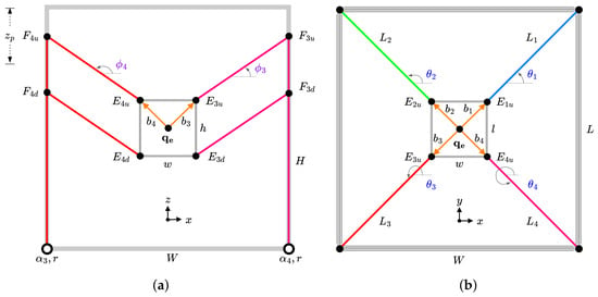
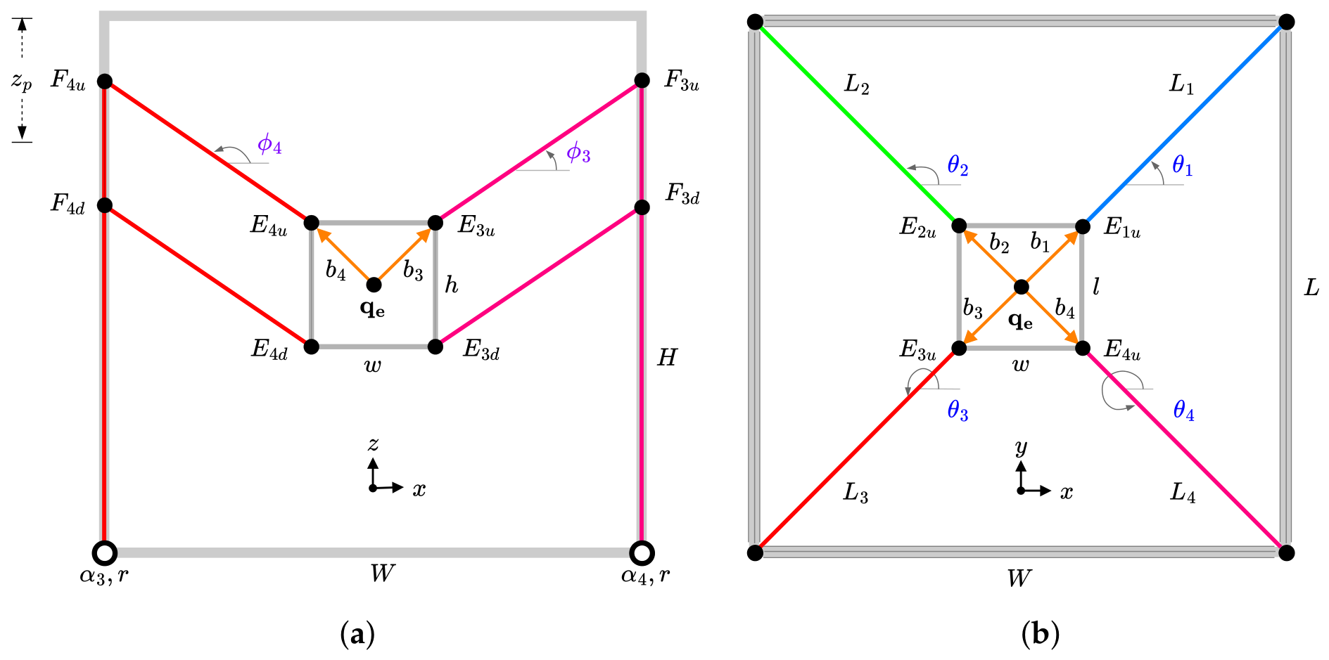
The coordinates depend on the height of the proximal anchoring points, , introducing an additional degree-of-freedom that enables robot reconfiguration. Figure 5 illustrates the nomenclature used throughout this work, where the angles are defined in the -plane and the angles in the -plane.
Figure 5.
Nomenclature of the AgroCableBot mathematical model: (a) front view and (b) top view. The figure shows the frame anchoring points , the end-effector anchoring points , and the angles and employed in the kinematics formulation. Adapted from [34].
Inverse kinematics is used to determine the joint coordinates required to achieve a desired end-effector position and orientation, , together with a specified value of . As detailed in [34], the general functional relationship is given by
Let denote the initial length of cable i corresponding to a reference end-effector pose . This length is computed as
For an arbitrary end-effector pose, the current cable length is obtained as
The joint coordinates required to reach such a pose are expressed as
Therefore, the inverse kinematics formulation can be summarized as
where the sign indicates whether a positive motor rotation produces an increase or a decrease in cable length, r = 44.2 mm is the drum radius, and .
The robot statics are derived from the equilibrium of forces and moments acting on the end-effector [37]. This equilibrium condition is expressed as
where is the structure matrix (the transpose of the Jacobian matrix), is the cable tension vector, where Ti is the total tension of the cable pair i, and represents the external wrench acting on the end-effector, with = 3 kg.
The cable tensions must satisfy (), with N as in the workspace analysis of [34], to ensure that all cables remain taut and that the robot preserves its controllability.
The structure matrix is defined as
where are the unit vectors along the direction of each cable, defined as
is the position vector of the anchor point with respect to the center of the end-effector, and is the rotation matrix about the z-axis:
Because the end-effector can only rotate about the z-axis, only the three force components and the moment about the z-axis are kept from Equation (7), so is a matrix, consistent with . This formulation enables the analysis of the kinematics and static behavior of AgroCableBot and provides the foundation for the control algorithms and position estimation procedures presented in the following sections.
3.2. End-Effector Detection and Position Estimation
The computer vision system provides the sensing layer required to align the robot’s physical workspace with its digital representation and to estimate the three-dimensional position of the end-effector. The proposed approach compensates for perspective distortions introduced by the camera placement and establishes a consistent mapping between image coordinates and the robot’s Cartesian workspace. The resulting position estimate is used both for the initial calibration of the end-effector and as feedback for trajectory monitoring and closed-loop control. The estimation procedure consists of four stages: marker detection, centroid localization, geometric transformation, and end-effector position estimation.
3.2.1. Marker Detection
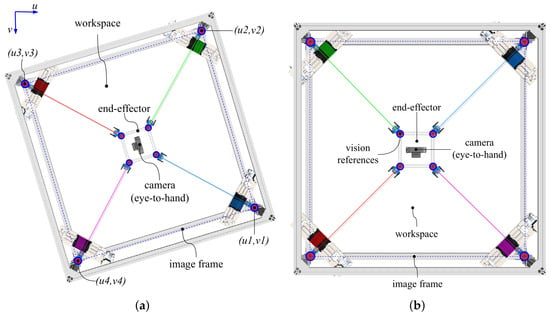
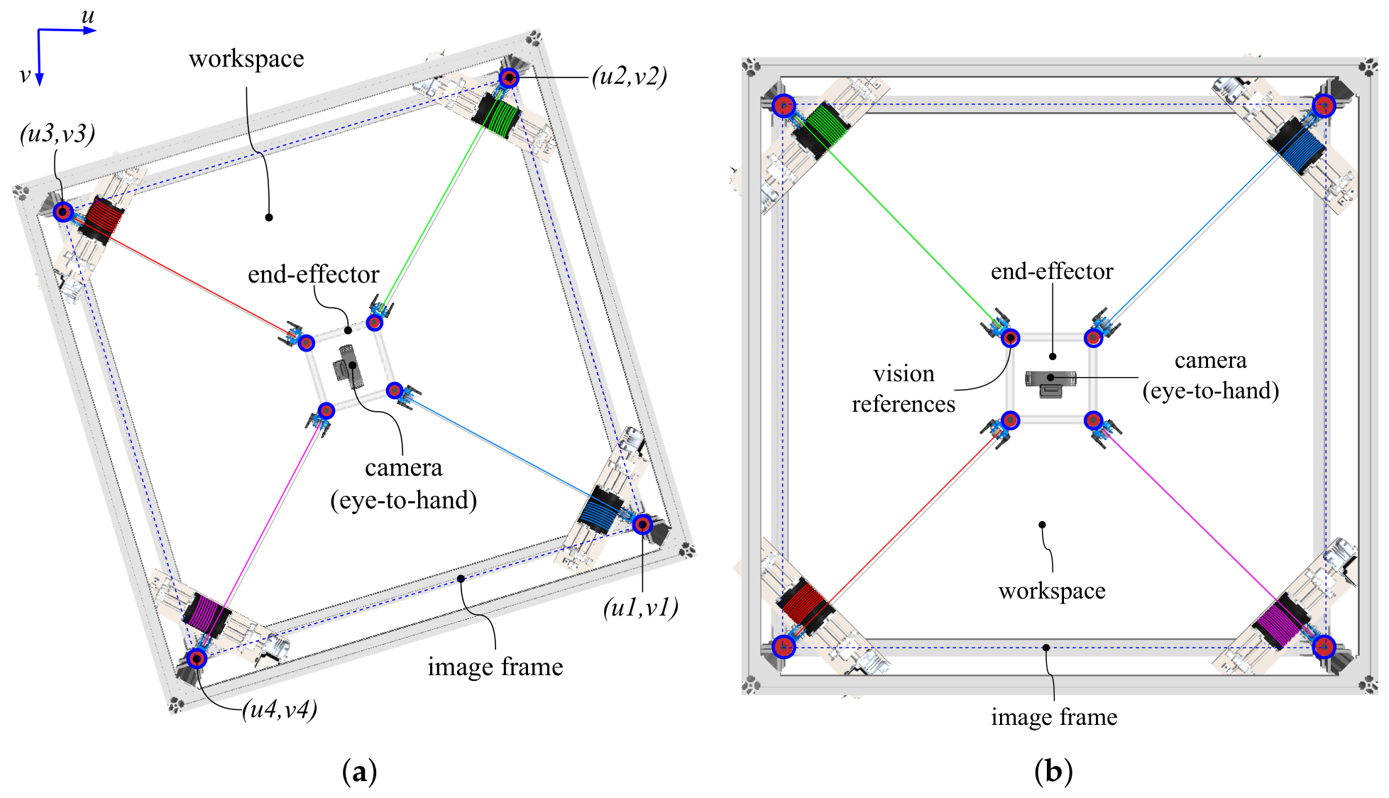
Marker detection is based on the identification of eight red circular markers, four on the frame and four on the end-effector (Figure 6), selected for their high contrast with the agricultural environment, which is predominantly characterized by green vegetation. The acquired image is segmented in the HSV color space using a thresholding operation, generating a binary mask corresponding to the regions of interest.
Figure 6.
Perspective transformation applied to the image captured by the ETH camera: (a) original image affected by perspective distortion, and (b) corrected image aligned with the robot workspace.
To eliminate small spurious regions and fill discontinuities caused by image noise or robot components such as cables, the binary mask is processed through erosion and dilation morphological operations. Finally, the marker contours are extracted for subsequent analysis following the procedure described in [36].
3.2.2. Centroid Localization
Once the marker contours have been extracted, the image coordinates of the four marker centroids are computed using image geometric moments. These centroids constitute the visual features employed to define the image reference frame and estimate the end-effector position.
The two-dimensional image moments are defined as
whereas the centroid coordinates of each marker are computed as
3.2.3. Geometric Transformation
To establish a correspondence between the acquired image and the robot workspace, a perspective transformation (homography) is applied to compensate for perspective, rotation, translation, and scaling effects. Following [38] the perspective transformation is expressed as
where denotes the original image coordinates, and represents the transformed coordinates, obtained by dividing the first two components by the scale factor s.
The transformation matrix is computed from the four frame markers, using their known positions in the robot workspace and their corresponding image coordinates. As a result, a geometrically aligned image with a 1:1 aspect ratio is obtained, as illustrated in Figure 6. Because the frame markers are located on the mobile pulleys, they move with the anchor height . The transformation is therefore recomputed after each reconfiguration, so the calibration plane follows the operating plane of the end-effector.
3.2.4. End-Effector Position Estimation
To estimate the end-effector position, four red circular markers are placed collinearly with the cable attachment points located at the pulley rotation axes of the end-effector. These markers are detected and localized using the same procedure described in the previous subsections.
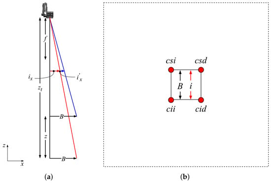
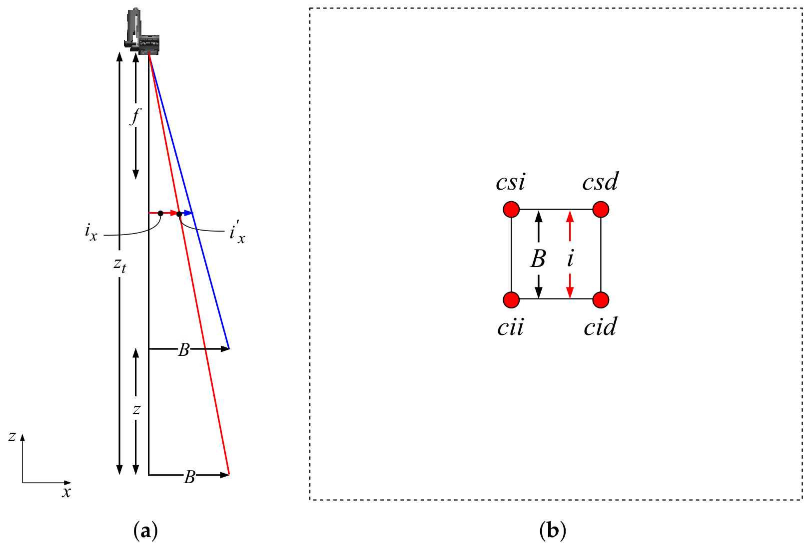
Subsequently, a pinhole camera model is employed to estimate the end-effector height z and its horizontal coordinates , as illustrated in Figure 7.
Figure 7.
Geometric model used for end-effector position estimation using the ETH camera: (a) height estimation based on similar triangles, and (b) conversion between image coordinates and physical workspace coordinates.
The height is obtained from the relationship of similar triangles projected onto the image plane:
where denotes the reference area measured at a known height during calibration, using a calibration board with a chessboard pattern, and corresponds to the area enclosed by the centroids of the four end-effector markers.
To convert image coordinates into metric coordinates, a pixel-to-metric scale factor (mm/pixel) is obtained from the transformed image as the ratio between the known distance between the frame markers and their distance in pixels. ks is constant for a given configuration (approximately 1.36 mm/pixel in the experiments) and is valid at the plane of the frame markers. Since this plane moves with and the end-effector operates at the same height, the perspective scale error is small. A residual error remains because the end-effector markers are located 30 mm from the plane of the frame markers along the vertical direction. With the camera located 2270 mm above the floor, this offset produces a scale error of 1.6%, 1.8% and 2.2% at end-effector heights of 400, 600, and 900 mm, respectively. The resulting error is zero at the center of the workspace and reaches 5 to 8 mm at the edges of the 600 × 600 mm trajectories. Because the controller uses the same measurement, this error is not visible in the tracking metrics of Section 4; it changes the real size of the executed trajectory and can be compensated with a height-dependent correction factor in future implementations. This parameter establishes the relationship between image pixels and physical coordinates in the robot workspace.
First, the geometric center of the four detected markers is computed as
where represents the image coordinates of the individual markers, measured with respect to the image center, which corresponds to the center of the workspace.
The horizontal coordinates of the end-effector are then calculated as
Finally, the estimated end-effector position with respect to the home reference position is defined by
where denotes the vertical offset between the reference plane and the point of interest located on the end-effector.
Based on this estimated position, the cable lengths required by the robot controller are computed. For example, the position of the end-effector anchor point corresponding to quadrant 1 is expressed as
and the corresponding cable length is , as in Equation (3).
The information provided by the computer vision system constitutes the visual sensing feedback of the control loop, enabling continuous estimation of the end-effector position and real-time correction of positioning errors during trajectory execution. The estimated position is continuously compared with the desired Cartesian trajectory, and the resulting position error is used by the controller to generate corrective commands for the cable actuators.
With this configuration, the resolution of the position measurement is approximately 1.36 mm in the -plane and 0.65 mm along the z-axis. With an earlier prototype and a similar vision method, the static precision at the home position, evaluated according to ISO 5725-1 [39], was 0.04 mm in x, 0.05 mm in y and 0.44 mm in z [36]. The method assumes that the plane of the end-effector markers remains parallel to the image plane; a tilt of the end-effector changes AEF and introduces an error in the estimated height. In AgroCableBot, this error is small because the parallel cable pairs keep the end-effector horizontal.
3.3. Kinematics Control System
The end-effector motion can be described in Cartesian space by the vector , or in robot joint space by . The objective of the control system is to ensure that the end-effector accurately follows a desired trajectory while maintaining the cable tensions within the allowable operating range .
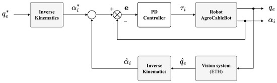
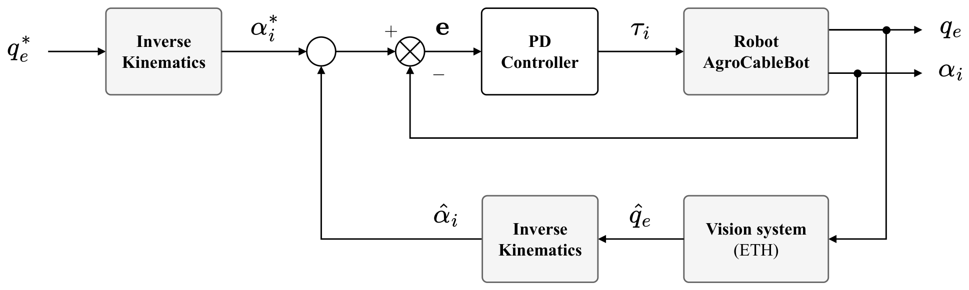
In this work, AgroCableBot is controlled in the joint space, as illustrated in Figure 8. This strategy provides a simple and robust implementation and facilitates direct integration with the actuation system. For each desired Cartesian reference , the inverse kinematic model generates the corresponding joint reference .
Figure 8.
Vision-based sensing and joint-space control architecture implemented in AgroCableBot. The desired Cartesian pose is converted into joint references through inverse kinematics. In the inner loop, each PD controller compares the joint reference with the encoder angle; in the outer loop, the difference between the desired joint references and the joint coordinates estimated by the vision system (ETH camera) is used to correct the joint references.
The dynamic model of AgroCableBot was developed in [34] under the assumption of massless and rigid cables, which is valid because of the high cable tensions obtained with the reconfiguration. The dynamics of each actuator, composed of the motor, the reducer and the drum, is given by
where J is the rotor inertia, the viscous friction coefficient, r the drum radius, and the motor torque. The dynamics model of the end-effector is
with , where is the end-effector mass and its moment of inertia about the z-axis. The combination of both equations gives the dynamic model of the robot in joint coordinates [34]:
In [34], this model was used to simulate the robot and validate the joint-space control scheme. In the experiments of this work, the controller does not use the dynamic model to compute the motor torques. The trajectories are generated using inverse kinematics, and the control is performed with independent joint controllers and vision feedback.
The controller block consists of a diagonal matrix whose diagonal elements correspond to four independent PID position controllers, one for each motor, as proposed in [34]. In the actuator model of Equation (18), the cable tension acts on each motor only as a load torque . In AgroCableBot, this coupling is reduced by the self-locking worm-gear reducer and by the low speeds of the agricultural trajectories, so the four axes can be controlled independently. The four controllers use the same gains, which were tuned experimentally: , and , with a control period of 1 ms. The integral gain was set to zero, so each controller acts as a PD controller. The steady-state positioning error is corrected by the outer vision loop, and the self-locking reducer prevents the cable load from back-driving the motors.
Two feedback loops are used, as shown in Figure 8. In the inner loop, each controller compares the joint reference with the motor angle measured by the encoder. In the outer loop, a vision-based closed-loop feedback system is implemented using the computer vision system to estimate the end-effector pose . The estimated pose is subsequently processed through the inverse kinematic model to obtain the corresponding estimated joint coordinates
which are continuously compared with the desired joint references . The resulting joint-position errors are used to correct the references of the independent PID controllers, which generate corrective commands for the actuators to compensate for positioning deviations during trajectory execution. The vision loop runs at the camera frame rate of 30 fps.
Additionally, the vision-based sensing system is employed during the initialization stage to automatically calibrate the end-effector and determine the robot home position, as described in [34,35,36].
4. Results
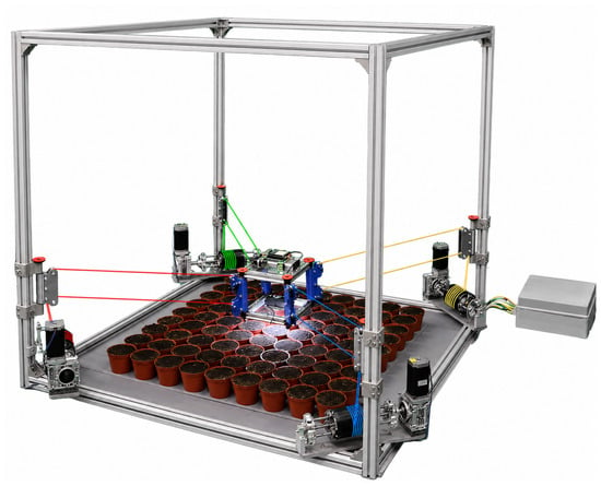
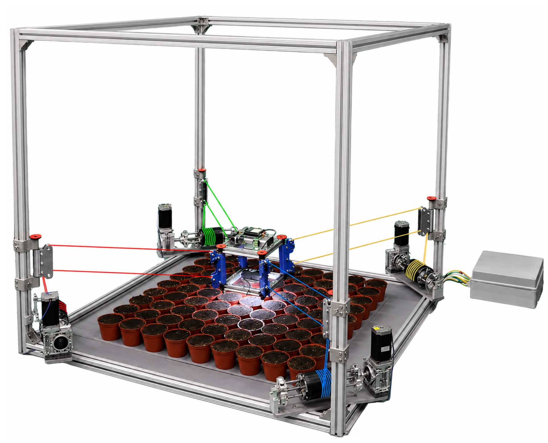
To experimentally validate the performance of the AgroCableBot robot, a series of experiments were conducted to evaluate the vision-based sensing system, the end-effector calibration procedure, and the trajectory tracking capability for representative agricultural applications, with particular emphasis on crop monitoring and localized positioning operations. The experiments focused on end-effector detection and position estimation, trajectory tracking, and positioning accuracy using vision-based feedback. Figure 9 shows the experimental prototype of the robot and its main subsystems.
Figure 9.
Experimental prototype of the AgroCableBot robot used for validation, consisting of the fixed frame, four cable collection systems, the reconfigurable pulley system, the end-effector, the electronic control unit, and the vision-based sensing system.
The experimental conditions are summarized in Table 2. Each trajectory was executed with a different anchor height , with the end-effector moving at the same height as the anchor points. All positions were measured with the vision system described in Section 3.2. The tracking performance was evaluated using the root mean square error (RMSE) along each axis, the three-dimensional RMSE, the 95th percentile (P95), and the maximum error. The results were judged against the requirements of the agricultural task: the inspection camera must be positioned over each plant of a seedling tray with a pot spacing of 50 mm, so errors of a few millimeters are acceptable.
Table 2.
Experimental conditions.
4.1. Vision-Based Sensing and End-Effector Calibration
The vision-based sensing system detects both the robot frame and the end-effector using a ETH camera, Logitech Brio. The ETH camera provides Ultra HD 4K images with a resolution of 4096 × 2160 pixels at 30 fps, enabling real-time estimation of the end-effector pose, automatic calibration of its initial position, and continuous monitoring of trajectory execution throughout all experiments.
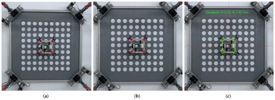
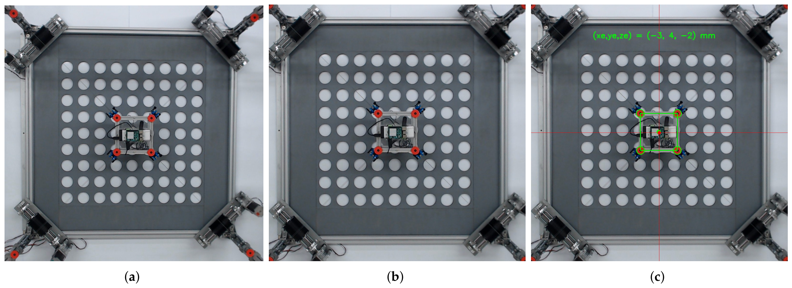
Figure 10 illustrates the end-effector detection procedure, which establishes the robot workspace reference frame and computes the perspective transformation described in Section 3.2. First, an image of the robot is acquired by the ETH camera (Figure 10a). Next, four circular reference markers located at the pulley rotation axes of the robot frame are detected. These markers define the workspace boundaries and are used to compute the perspective transformation of the -plane (Figure 10b). Finally, the reference markers attached to the end-effector are detected, allowing its position to be estimated within the workspace (Figure 10c).
Figure 10.
End-effector detection process: (a) image captured by the ETH camera; (b) detection of the frame reference markers and perspective transformation of the -plane; (c) detection and position estimation of the end-effector.
The end-effector is calibrated by moving it to the home position, defined as the configuration in which all cable lengths are equal and the end-effector is centered within the -plane. The home position is iteratively adjusted until the detected reference markers coincide with their predefined image coordinates within a tolerance of one pixel (approximately 1.4 mm). This configuration establishes the initial reference for all subsequent trajectory tracking experiments.
Throughout all experiments, the vision-based sensing system continuously estimated the end-effector position and provided visual feedback to supervise trajectory execution and detect deviations from the desired reference. The integration of the vision system with the motion controller enabled real-time correction of positioning errors, thereby improving the overall positioning accuracy of the AgroCableBot robot.
4.2. End-Effector Trajectory Tracking
To experimentally evaluate the trajectory tracking capability of the AgroCableBot robot, both basic geometric trajectories and representative agricultural trajectories were implemented. All trajectories were generated using Bézier curves and discretized into uniformly spaced reference points, ensuring smooth transitions between consecutive segments while minimizing abrupt variations in the end-effector velocity.
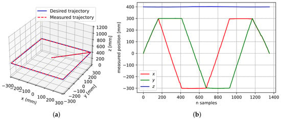
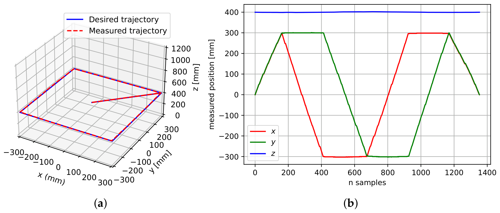
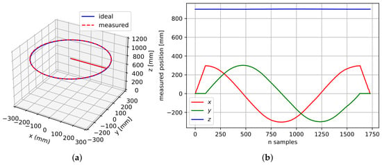
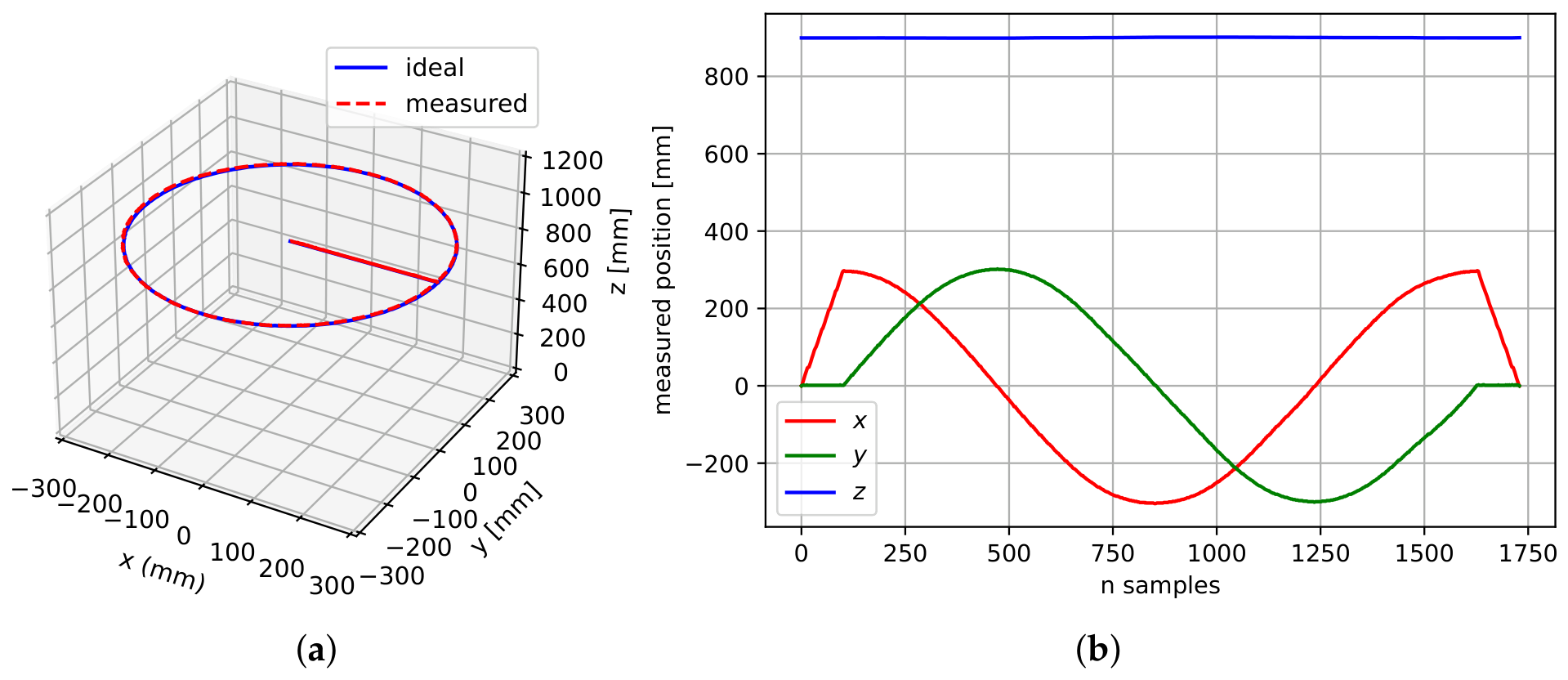
Figure 11, Figure 12 and Figure 13 illustrate the execution of the experimental trajectories at different end-effector heights and anchor heights (Table 2). In particular, Figure 11a presents the desired and measured square trajectories of the end-effector in the -plane. Figure 11b shows the temporal evolution of the corresponding position components, allowing for the dynamic behavior and motion smoothness achieved by the Bézier-based trajectory generation to be evaluated.
Figure 11.
Experimental tracking of a square trajectory: (a) Desired and measured trajectory in the -plane ( mm, mm). (b) Temporal evolution of the desired and measured end-effector positions along the x, y, and z directions.
Figure 12.
Experimental tracking of a circular trajectory: (a) Desired and measured trajectory in the -plane ( mm, mm). (b) Temporal evolution of the desired and measured end-effector positions along the x, y, and z directions.
Figure 13.
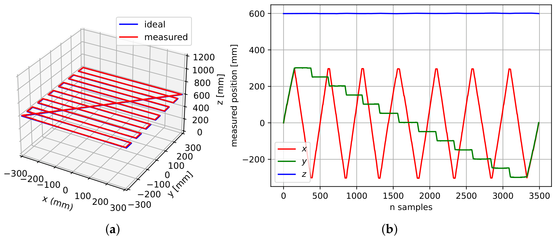
Experimental tracking of a seedling inspection trajectory: (a) Desired and measured trajectory in the -plane ( mm). (b) Temporal evolution of the desired and measured end-effector positions along the x, y, and z directions.
The measured square trajectory closely follows the desired path, with only small deviations observed mainly at the square corners. This behavior is consistent with the redistribution of cable tensions during abrupt changes in the direction of motion and with the inherent elasticity of cable-driven systems. In addition, these deviations are associated with the simultaneous variation in the lengths of multiple cables during the transitions between consecutive trajectory segments.
The circular trajectory was tracked continuously and stably, without noticeable discontinuities or significant oscillations of the end-effector (see Figure 12). The close agreement between the desired and measured trajectories demonstrates the capability of the system to execute smooth motions along paths with constant curvature. These results indicate that the inverse kinematic controller, together with the independent PID controllers implemented for each actuator, allows smooth tracking of continuous-curvature paths at an anchor height of 900 mm.
Finally, the robot was validated using a trajectory representative of a real agricultural task. The end-effector followed a raster path of 13 rows spaced 50 mm over a seedling tray, covering mm at a constant height of 600 mm (see Figure 13). This experiment validates the capability of the proposed system to perform repetitive inspection tasks over the seedling tray while taking advantage of the enlarged workspace achieved through the vertical reconfiguration of the proximal cable attachment points.
Overall, the experimental results demonstrate that the proposed control architecture, combining inverse kinematics, independent PID position controllers for each actuator, and vision-based feedback, enables smooth and stable Cartesian trajectory tracking. The small tracking deviations are mainly concentrated in regions involving abrupt changes in motion direction, whereas continuous-curvature trajectories exhibit an almost perfect overlap between the desired and measured paths. A quantitative analysis of these observations is presented in the following subsection through positioning error metrics.
4.3. End-Effector Positioning Accuracy
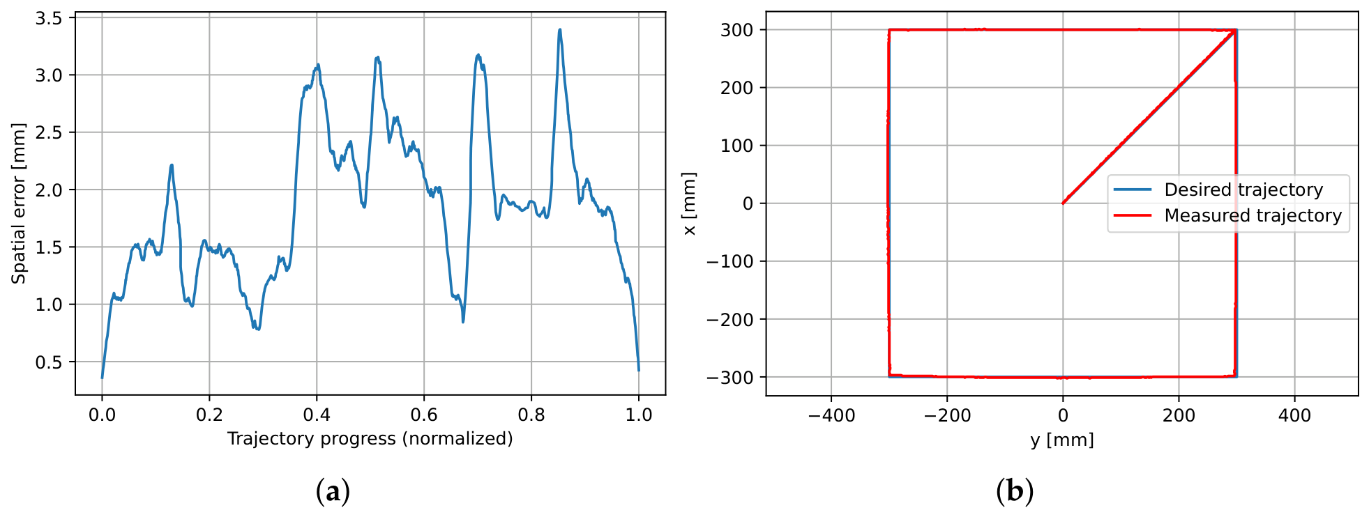
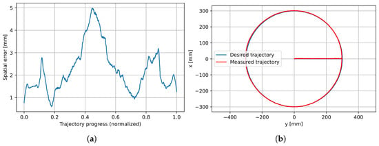
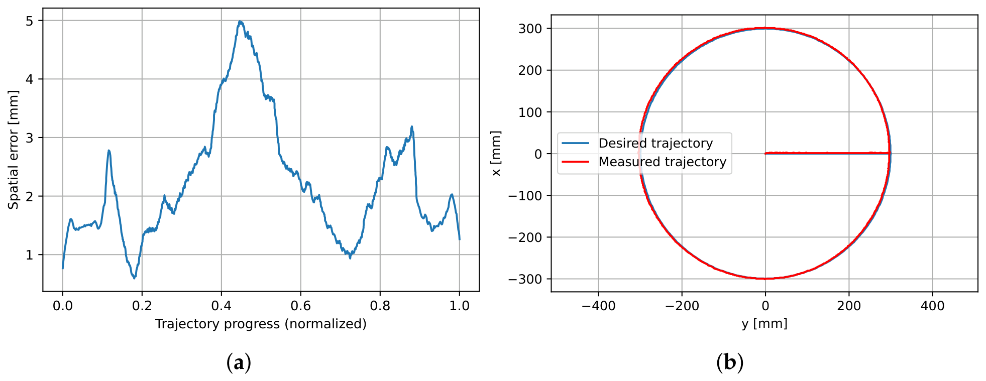
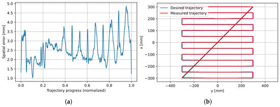
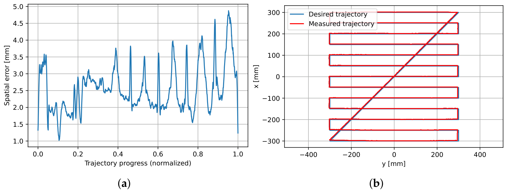
Positioning accuracy was evaluated by computing the minimum Euclidean distance between each measured trajectory point and the reference trajectory. To this end, the reference trajectory was densified with a spacing of 0.05 mm, and a nearest-neighbor search based on a KD-tree algorithm was employed to determine the spatial tracking error (Figure 14, Figure 15 and Figure 16). For each experiment, the tracking errors along the x, y, and z directions were computed, along with the root mean square error (RMSE), the 95th percentile (P95), and the maximum error (Table 3). These metrics provide a quantitative assessment of the control system performance during the execution of different trajectories within its workspace.
Figure 14.
Experimental tracking of a square trajectory: (a) Spatial tracking error along the square trajectory. (b) Desired and measured Cartesian trajectory in the -plane ( mm). The spatial error is smoothed with a Savitzky–Golay filter (window 51, order 3) for visualization; the metrics in Table 3 are computed from the unfiltered error.
Figure 15.
Experimental tracking of a circle trajectory: (a) Spatial tracking error along the circle trajectory. (b) Desired and measured Cartesian trajectory in the -plane ( mm). The spatial error is smoothed with a Savitzky–Golay filter (window 51, order 3) for visualization; the metrics in Table 3 are computed from the unfiltered error.
Figure 16.
Experimental tracking of a seedling inspection trajectory: (a) Spatial tracking error along the trajectory. (b) Desired and measured Cartesian trajectory in the -plane ( mm). The spatial error is smoothed with a Savitzky–Golay filter (window 51, order 3) for visualization; the metrics in Table 3 are computed from the unfiltered error.
Table 3.
Positioning accuracy metrics obtained from the experimental trajectory tracking tests.
For reference, positioning errors of 10 to 40 mm are reported for large-scale cable-driven parallel robots [37]. Since these robots are much larger, a fair comparison requires normalizing by the workspace size: the 3D RMSE obtained here corresponds to about 0.3% of the 800 mm side of the admissible workspace. AgroCableBot achieved RMSE values below 2 mm along the horizontal axes and a spatial RMSE below 3 mm for all evaluated trajectories while simultaneously maintaining a large and reconfigurable workspace. These results indicate that the proposed architecture provides high positioning accuracy without compromising the workspace enlargement enabled by the reconfigurable design, making it suitable for precision agriculture applications such as crop monitoring, localized irrigation, and automated seeding.
The positioning errors along the three Cartesian directions remained within the same order of magnitude (approximately 1–2 mm). The small differences observed among the evaluated trajectories are mainly attributed to cable tension redistribution during motion and to the uncertainty associated with the vision-based estimation of the end-effector position. Because each trajectory was executed at a different anchor height, the differences between trajectories combine the effects of the path geometry and of the height.
Although the evaluated trajectories exhibit different geometries, the spatial RMSE remained below 3 mm in all cases. The P95 values, all below 5 mm, indicate that 95% of the trajectory points were tracked with positioning errors below 5 mm. Furthermore, the relatively small separation between the RMSE and P95 values indicates that large tracking deviations were limited to a small fraction of the trajectory points. In all experiments, the maximum positioning error did not exceed 6.0 mm. Overall, these results support the validity of the proposed kinematic model and demonstrate the effectiveness of the control strategy based on inverse kinematics, independent joint control of each actuator, and vision-based feedback, enabling the execution of agricultural trajectories with high positioning accuracy within the reconfigurable workspace.
Each trajectory was executed once. To characterize the consistency of the tracking error within each run, the 3D RMSE was computed for each segment of the trajectories. The variability between segments was 1.88 ± 0.57 mm for the four sides of the square, 2.54 ± 0.89 mm for the four quadrants of the circle and 2.28 ± 0.40 mm for the 13 rows of the inspection trajectory. The error increased near direction changes: 2.24 mm near the corners of the square compared with 1.92 mm along the sides, and 3.15 mm at the row ends of the inspection trajectory compared with 2.28 mm at the center of the rows. These peaks correspond to the corners in Figure 14a, where the Bézier transition changes the direction of motion and the cable lengths change simultaneously. The error also showed a position-dependent trend: in the inspection trajectory, the row RMSE increased from 1.54 mm at y = +300 mm to 3.01 mm at y = −300 mm. This suggests a systematic component related to calibration and geometric modeling, rather than random noise.
5. Discussion
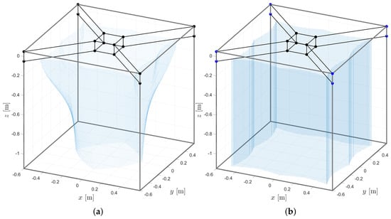
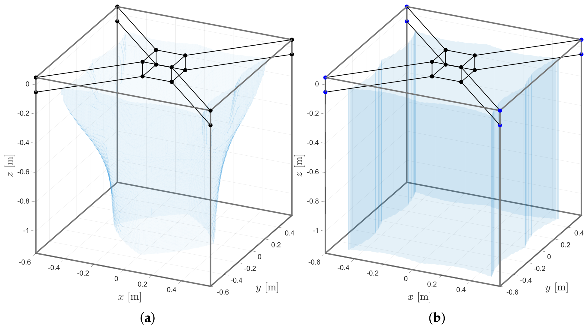
The obtained results allow the impact of the proposed reconfigurable architecture to be analyzed from kinematic, static, and experimental perspectives. First, the simulation results show that, for a suspended conventional CDPR configuration, increasing the minimum cable tension from 0 to 20 N progressively reduces the feasible workspace from approximately 88% to 14% of the geometrically admissible workspace [34]. This finding is consistent with previous studies reporting the strong dependence of the feasible workspace of CDPRs on cable tension constraints [37].
The proposed vertical reconfiguration of the proximal cable attachment points introduces a controlled trade-off between workspace and cable tension. By selecting an appropriate value for the proximal anchor height , the robot operates in a higher-tension regime, thereby enlarging the wrench-feasible workspace while satisfying the prescribed cable tension constraints. The workspace analyzed in [34] corresponds to the translational wrench-feasible workspace under a fixed end-effector orientation. The feasible region was computed through a uniform Cartesian discretization, testing at each sampled pose whether a cable tension distribution satisfying the prescribed tension bounds exists. For N, the wrench-feasible workspace increases from approximately 58% to 100% of the geometrically admissible workspace [34]. This substantial increase in feasible workspace demonstrates that geometric reconfiguration is an effective strategy for overcoming one of the major limitations of CDPRs in large-scale agricultural applications. In this work, the robot was operated at three anchor heights ( = 400, 600 and 900 mm), and the trajectories covered 600 × 600 mm in the -plane at each height. In additional tests, the end-effector reached 720 × 720 mm, which corresponds to 81% of the admissible area in the -plane. The cable tensions were not measured in the experiments; therefore, the tension feasibility of the executed trajectories relies on the model of [34].
Figure 17 compares the wrench-feasible workspace of the conventional and the reconfigured configurations computed in [34].
Figure 17.
Wrench-feasible workspace for N: (a) conventional suspended configuration with fixed anchor points; (b) reconfigurable configuration of AgroCableBot. Adapted from [34].
As a direct consequence of this reconfiguration, the operating cable tensions predicted by the simulations in [34] increase to approximately 50–260 N, compared with 10–50 N in the conventional configuration. Although this requires greater mechanical effort from both the actuators and the cables, it also increases the apparent stiffness of the system, reduces cable deformation caused by cable elasticity, and improves end-effector stability. With the prototype parameters, a tension of 250 N in a cable pair requires a torque of about 11 Nm at the drum (r = 44.2 mm) and about 2.2 Nm at the motor, assuming a worm-gear efficiency of 0.5, typical of self-locking worm gears. This is within the 3 Nm of the motors. The experimental validation showed a spatial RMSE below 3 mm during both geometric and agricultural trajectory tracking.
Experimentally, the vision-based sensing system provided stable end-effector pose estimation and enabled the implementation of a vision-based feedback control strategy. During the evaluated trajectory tracking experiments, the system achieved RMSE values below 2 mm along the horizontal axes and a spatial RMSE below 3 mm, while the 95th percentile remained below 5 mm and the maximum tracking error did not exceed 6.0 mm. These values are measured with the same vision system used for feedback, so they describe the tracking error with respect to the vision measurement. The main systematic error of this measurement is the residual scale error described in Section 3.2.4, which is between 1.6% and 2.2% and reaches 5 to 8 mm at the edges of the trajectories. Even including this error, the positioning error is well below the 50 mm spacing between pots, so the proposed vision-based positioning system provides sufficient accuracy for agricultural applications requiring repetitive motions and precise localized positioning.
The experiments also demonstrated consistent system performance across trajectories with different geometric characteristics. Although trajectories involving abrupt direction changes are expected to produce variations in cable tension distribution, the spatial RMSE remained below 3 mm in all evaluated cases. These results indicate that the proposed control strategy, based on inverse kinematics, independent joint control of each actuator, and visual feedback, performs consistently under different trajectory conditions. The segment analysis showed that the error increases at direction changes and towards one side of the workspace, which indicates a systematic component that could be reduced with a finer calibration of the geometric parameters. Since each trajectory was executed at a different anchor height, the effect of the height cannot be separated from the effect of the path geometry with the present data.
The use of an Eye-to-Hand camera eliminated the need to install additional sensors on the end-effector while simultaneously enabling both the initial calibration procedure and continuous end-effector position estimation. This approach simplifies the robot instrumentation and facilitates its deployment in agricultural environments, where robustness, low cost, and ease of implementation are important practical considerations.
Overall, the results demonstrate that the proposed reconfigurable architecture effectively addresses one of the main limitations of cable-driven parallel robots for agricultural applications: the limited ratio between the usable workspace and the size of the structure. The combination of geometric reconfiguration, vision-based kinematic control, and accurate trajectory tracking provides a suitable robotic platform for automating agricultural tasks such as crop monitoring, precision irrigation, and automated seeding in protected cultivation environments.
The scalability of the system depends mainly on the vision system, the actuators, and the cables. For a given camera and image size, the measurement resolution decreases in proportion to the workspace size: the current resolution of 1.36 mm per pixel for a 0.8 m workspace would become about 8.5 mm per pixel for a 5 m workspace. A larger system would therefore require a higher-resolution camera, several cameras, or additional sensors. The cable tensions grow with the end-effector mass, and the required motor torque increases with the tension and the drum radius, so larger systems would need higher-torque motors or higher reduction ratios. The cable sag, which is about 0.1 mm for the current frame at 5 N, grows with the square of the cable length (about 2 mm for a 5 m cable at the same tension) and remains negligible at the operating tensions of the reconfigured configuration. The cable elongation also increases with cable length, so longer cables would require stiffer cables or a compensation for the elongation in the kinematic model. Finally, the vertical reconfiguration, which is manual in the current prototype, would need to be motorized in larger systems.
Although AgroCableBot was designed for protected agriculture, the same architecture can be used in other applications that require positioning a sensor or a light tool over a large horizontal area with a compact frame. Examples include plant phenotyping in growth chambers and vertical farms, inspection and inventory of shelves in warehouses, laboratory automation for imaging samples or culture trays, and inspection of flat surfaces. In all these cases, the vertical reconfiguration allows the working height to be adapted to the task while keeping the cables in tension.
Although the experimental results were satisfactory, the present study has several limitations. First, the proposed system depends on adequate illumination conditions for reliable monocular vision-based positioning. Second, the positioning errors were measured with the same vision system used for feedback; an external reference, such as a laser tracker or a motion capture system, was not available. Third, the cable tensions were not measured, and each trajectory was executed once at a single anchor height. Fourth, the experimental validation was conducted using a lightweight end-effector. Therefore, future work should investigate the robot performance under larger payloads and external disturbances generated during physical interaction with crops, include repeated trials following ISO 9283 [40] with an external measurement system, and measure the cable tensions to verify the minimum tension experimentally.
6. Conclusions
This paper presents the experimental validation of AgroCableBot, a reconfigurable cable-driven parallel robot (CDPR) for precision agriculture, whose design and simulation were introduced in [34]. The robot incorporates a vertical reconfiguration mechanism for the proximal cable attachment points, which, according to the simulations in [34], increases the wrench-feasible workspace from approximately 58% to 100% of the geometrically admissible workspace for N. The main contributions of this work are the physical implementation of the reconfigurable robot, the integration of a vision-based sensing system for calibration and closed-loop control, and the experimental evaluation of trajectory tracking at three anchor heights.
The experiments showed that the robot can execute geometric and agricultural trajectories at anchor heights of 400, 600 and 900 mm, covering 600 × 600 mm in the -plane, with a vision-measured 3D RMSE between 1.9 and 2.6 mm, a 95th-percentile error below 4.5 mm and a maximum error of 6.0 mm. The error increased at direction changes and showed a position-dependent trend, and the residual scale error of the vision measurement was estimated at 1.6–2.2%. These accuracy levels are adequate for positioning an inspection camera over a seedling tray with a pot spacing of 50 mm.
The vision-based sensing system enabled both the initial calibration of the robot and continuous end-effector position estimation for closed-loop control, providing the feedback required for accurate trajectory tracking. The Eye-to-Hand sensing configuration also simplifies end-effector instrumentation while providing a global measurement of its position within the workspace. The experimental results obtained across trajectories with different geometric characteristics further demonstrate the consistent performance of the proposed sensing and control architecture.
Overall, the results of [34] and of this work indicate that geometric reconfiguration can effectively address the limited feasible workspace of suspended conventional CDPRs while maintaining high positioning accuracy. The combination of reconfigurable cable attachment points, reconfiguration-aware kinematic modeling, vision-based sensing, and closed-loop control provides a practical foundation for the development of agricultural robotic platforms capable of supporting autonomous crop monitoring and other localized operations in protected cultivation environments.
The main challenges for the next stages are the validation of the positioning accuracy with an external measurement system, the measurement of the cable tensions to verify the minimum tension experimentally, repeated trials following ISO 9283 [40], the compensation of the residual scale error of the vision system, and the operation with heavier end-effectors and in contact with the plants.
Future Work
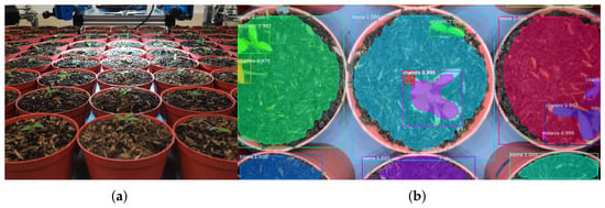
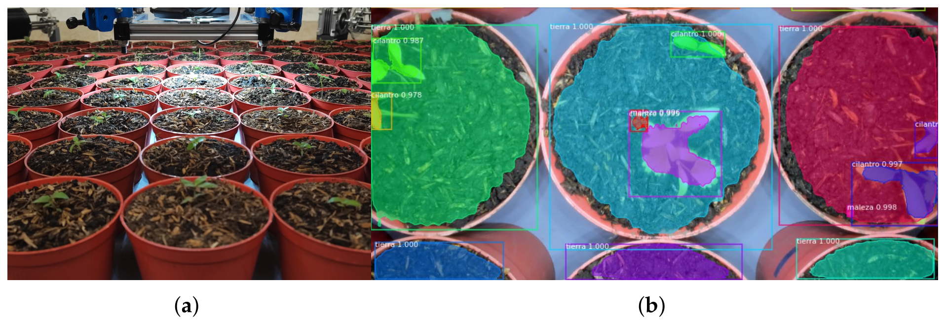
Future research will focus on integrating higher-resolution cameras and spectral imaging sensors to enable the real-time acquisition of high-resolution and multimodal crop information. In addition, deep learning-based artificial intelligence algorithms will be investigated for the automatic segmentation, classification, and detection of seedlings, weeds, and crop phenological stages, as shown in Figure 18.
Figure 18.
Future computer vision and artificial intelligence framework for AgroCableBot: (a) potted coriander plants used as experimental agricultural targets. (b) Semantic segmentation and classification of soil, crop, and weeds for autonomous monitoring and precision agriculture applications.
At the system level, a data infrastructure will be developed to support the real-time acquisition, storage, and processing of crop phenotyping data, providing the computational basis for automated decision-making in precision agriculture applications. This infrastructure will enable the integration of multimodal sensing data with the robotic control system, facilitating the development of data-driven agricultural operations.
From the robotic system perspective, future work will motorize the vertical reconfiguration and investigate automatic reconfiguration strategies for the cable attachment points according to the agricultural task and the cable tension state, with the objective of simultaneously optimizing the workspace, structural stiffness, and energy consumption. Furthermore, dynamic models and advanced predictive and adaptive control strategies will be investigated to increase the robot’s operating speed, positioning accuracy, and robustness during the execution of complex agricultural tasks.
These developments are expected to further establish AgroCableBot as a versatile research platform for advanced precision agriculture, integrating cable-driven parallel robotics, vision-based sensing, spectral imaging, and artificial intelligence within a unified framework for autonomous crop monitoring, phenotyping, and management in protected cultivation environments.
Author Contributions
Conceptualization, A.G.-V. and M.J.G.-B.; methodology, A.G.-V. and M.J.G.-B.; software, A.G.-V. and M.J.G.-B.; validation, A.G.-V. and M.J.G.-B.; investigation, A.G.-V. and M.J.G.-B.; writing original draft preparation, A.G.-V. and M.J.G.-B.; supervision, A.G.-V. and M.J.G.-B.; project administration, A.G.-V. and M.J.G.-B.; funding acquisition, A.G.-V. and M.J.G.-B. All authors have read and agreed to the published version of the manuscript.
Funding
This research was funded by the Science for Peace and Security (SPS) Programme of the NATO organization by the grant G6001.
Data Availability Statement
The data presented in this study are available on request from the corresponding author.
Acknowledgments
During the preparation of this manuscript, the authors used ChatGPT (OpenAI) for language editing purposes, including grammar checking, improving English usage, and enhancing the clarity and readability of the text. The manuscript was written and scientifically developed by the authors, who reviewed and edited the entire manuscript and assume full responsibility for the accuracy, scientific validity, and integrity of its content.
Conflicts of Interest
The authors declare no conflicts of interest.
Abbreviations
The following abbreviations are used in this manuscript:
| CDPR | Cable-Driven Parallel Robot |
| DOF | degree-of-freedom |
| EIH | Eye-in-hand |
| ETH | Eye-to-hand |
| HSV | Hue, saturation, value |
| IMU | Inertial measurement unit |
| P95 | 95th percentile |
| PD | Proportional–derivative |
| PID | Proportional–integral–derivative |
| RMSE | Root mean square error |
| UHMWPE | Ultra-high-molecular-weight polyethylene |
| WFW | Wrench-Feasible Workspace |
Nomenclature
| Symbol | Description | Unit |
| End-effector pose | mm, rad | |
| Rotation of the end-effector about the z-axis | rad | |
| Motor angles | rad | |
| Height of the proximal anchor points | mm | |
| Anchor point i on the frame | mm | |
| Anchor point i on the end-effector | mm | |
| Position of with respect to the end-effector center | mm | |
| , | Current and initial length of cable i | mm |
| Vector of cable length variations | mm | |
| r | Drum radius (44.2 mm) | mm |
| Pulley radius | mm | |
| Structure matrix | – | |
| Unit vector along cable i | – | |
| Rotation matrix about the z-axis | – | |
| Tensions of the cable pairs | N | |
| , | Minimum and maximum cable tension | N |
| External wrench on the end-effector | N, N·m | |
| End-effector mass (3 kg) | kg | |
| End-effector moment of inertia about the z-axis | kg·m2 | |
| End-effector mass matrix | kg, kg·m2 | |
| J | Rotor inertia | kg·m2 |
| Viscous friction coefficient | N·m·s/rad | |
| Motor torque | N·m | |
| , , | Controller gains | – |
| Image coordinates | pixel | |
| Transformed image coordinates | pixel | |
| s | Scale factor of the perspective transformation | – |
| Image moments | – | |
| Marker centroid | pixel | |
| , | Mean image coordinates of the end-effector markers | pixel |
| Pixel-to-metric scale factor | mm/pixel | |
| Known reference height | mm | |
| Reference area at height | pixel2 | |
| Area enclosed by the end-effector marker centroids | pixel2 | |
| Vertical offset between the reference plane and the | mm | |
| end-effector point of interest | ||
| , | Desired pose and desired joint coordinates | mm, rad |
| , | Estimated pose and estimated joint coordinates | mm, rad |
References
- Hiller, M.; Fang, S.; Mielczarek, S.; Verhoeven, R.; Franitza, D. Design, analysis and realization of tendon-based parallel manipulators. Mech. Mach. Theory 2005, 40, 429–445. [Google Scholar] [CrossRef] [Scilit]
- Hamann, M.; Nüsse, P.M.; Winter, D.; Ament, C. Towards a Precise Cable-Driven Parallel Robot—A Model-Driven Parameter Identification Enhanced by Data-Driven Position Correction. In Cable-Driven Parallel Robots; Springer International Publishing: Berlin/Heidelberg, Germany, 2019; pp. 367–376. [Google Scholar] [CrossRef] [Scilit]
- Zitzewitz, J.V.; Rauter, G.; Steiner, R.; Brunschweiler, A.; Riener, R. A versatile wire robot concept as a haptic interface for sport simulation. In Proceedings of the 2009 IEEE International Conference on Robotics and Automation, Kobe, Japan, 12–17 May 2009; pp. 313–318. [Google Scholar] [CrossRef] [Scilit]
- Mao, Y.; Agrawal, S.K. Design of a Cable-Driven Arm Exoskeleton (CAREX) for Neural Rehabilitation. IEEE Trans. Robot. 2012, 28, 922–931. [Google Scholar] [CrossRef] [Scilit]
- Vallery, H.; Lutz, P.; von Zitzewitz, J.; Rauter, G.; Fritschi, M.; Everarts, C.; Ronsse, R.; Curt, A.; Bolliger, M. Multidirectional transparent support for overground gait training. In Proceedings of the 2013 IEEE 13th International Conference on Rehabilitation Robotics (ICORR), Seattle, WA, USA, 24–26 June 2013; pp. 1–7. [Google Scholar] [CrossRef] [Scilit] [PubMed]
- Castelli, G.; Ottaviano, E. Modelling and Simulation of a Cable-Based Parallel Manipulator as an Assisting Device. In Proceedings of the Computational Kinematics; Kecskeméthy, A., Müller, A., Eds.; Springer: Berlin/Heidelberg, Germany, 2009; pp. 17–24. [Google Scholar] [CrossRef] [Scilit]
- Castelli, G.; Ottaviano, E.; Rea, P. A Cartesian Cable-Suspended Robot for improving end-users’ mobility in an urban environment. Robot. Comput.-Integr. Manuf. 2014, 30, 335–343. [Google Scholar] [CrossRef] [Scilit]
- Wu, M.; Brown, G.L.; Kim, K.Y.A.; Kim, J.; Gordon, K.E. Gait variability following abrupt removal of external stabilization decreases with practice in incomplete spinal cord injury but increases in non-impaired individuals. J. Neuroeng. Rehabil. 2019, 16, 4. [Google Scholar] [CrossRef] [Scilit] [PubMed]
- Zou, Y.; Wang, N.; Wang, X.; Ma, H.; Liu, K. Design and Experimental Research of Movable Cable-Driven Lower Limb Rehabilitation Robot. IEEE Access 2019, 7, 2315–2326. [Google Scholar] [CrossRef] [Scilit]
- Heyden, T.; Woernle, C. Dynamics and flatness-based control of a kinematically undetermined cable suspension manipulator. Multibody Syst. Dyn. 2006, 16, 155–177. [Google Scholar] [CrossRef] [Scilit]
- Bruckmann, T.; Lalo, W.; Nguyen, K.; Salah, B. Development of a storage retrieval machine for high racks using a wire robot. In Proceedings of the International Design Engineering Technical Conferences and Computers and Information in Engineering Conference, Chicago, IL, USA, 12–15 August 2012; American Society of Mechanical Engineers: New York, NY, USA, 2012; Volume 4, pp. 771–780. [Google Scholar] [CrossRef] [Scilit]
- Voss, K.H.J.; van der Wijk, V.; Herder, J.L. Investigation of a Cable-Driven Parallel Mechanism for Interaction with a Variety of Surfaces, Applied to the Cleaning of Free-Form Buildings. In Proceedings of the Latest Advances in Robot Kinematics; Lenarcic, J., Husty, M., Eds.; Springer: Dordrecht, The Netherlands, 2012; pp. 261–268. [Google Scholar] [CrossRef] [Scilit]
- Voss, K.H.J.; van der Wijk, V.; Herder, J.L. A Cable-Driven Parallel Mechanism for the Interaction with Hemispherical Surfaces. In Proceedings of the New Trends in Mechanism and Machine Science; Viadero, F., Ceccarelli, M., Eds.; Springer: Dordrecht, The Netherlands, 2013; pp. 409–417. [Google Scholar] [CrossRef] [Scilit]
- Bosscher, P.; Williams, R.L.; Bryson, L.S.; Castro-Lacouture, D. Cable-suspended robotic contour crafting system. Autom. Constr. 2007, 17, 45–55. [Google Scholar] [CrossRef] [Scilit]
- Pott, A.; Meyer, C.; Verl, A. Large-scale assembly of solar power plants with parallel cable robots. In Proceedings of the ISR 2010 (41st International Symposium on Robotics) and ROBOTIK 2010 (6th German Conference on Robotics), Munich, Germany, 7–9 June 2010; VDE: Offenbach am Main, Germany, 2010; pp. 1–6. [Google Scholar]
- Lytle, A.; Proctor, F.; Saidi, K. Control of Cable Robots for Construction Applications. In Parallel Manipulators—Towards New Applications; Wu, H., Ed.; IntechOpen: London, UK, 2008; Chapter 1. [Google Scholar] [CrossRef] [Scilit] [PubMed][Green Version]
- Izard, J.B.; Gouttefarde, M.; Baradat, C.; Culla, D.; Sallé, D. Integration of a Parallel Cable-Driven Robot on an Existing Building Façade. In Cable-Driven Parallel Robots; Springer: Berlin/Heidelberg, Germany, 2013; pp. 149–164. [Google Scholar] [CrossRef] [Scilit]
- Zheng, Y.Q. Feedback Linearization Control of a Wire-Driven Parallel Support System in Wind Tunnels. In Proceedings of the Sixth International Conference on Intelligent Systems Design and Applications, Jian, China, 16–18 October 2006; Volume 3, pp. 9–13. [Google Scholar] [CrossRef] [Scilit]
- Xiao, Y.; Lin, Q.; Zheng, Y.; Liang, B. Model Aerodynamic Tests with a Wire-driven Parallel Suspension System in Low-speed Wind Tunnel. Chin. J. Aeronaut. 2010, 23, 393–400. [Google Scholar] [CrossRef] [Scilit]
- Sturm, C.; Wildan, L.; Bruckmann, T. Wire Robot Suspension Systems for Wind Tunnels. In Wind Tunnels and Experimental Fluid Dynamics Research; Lerner, J.C., Boldes, U., Eds.; IntechOpen: London, UK, 2011; Chapter 2. [Google Scholar] [CrossRef] [Scilit] [PubMed]
- Bauer, C. Device and Method for Detecting the Inventory of a Selling and/or Storing Device, and a Storage-Managing System Equipped with Said Device. WO Patent WO/2012/101248, 27 January 2012. [Google Scholar]
- Pott, A.; Mütherich, H.; Kraus, W.; Schmidt, V.; Miermeister, P.; Verl, A. IPAnema: A family of Cable-Driven Parallel Robots for Industrial Applications. In Cable-Driven Parallel Robots; Springer: Berlin/Heidelberg, Germany, 2013; pp. 119–134. [Google Scholar] [CrossRef] [Scilit]
- Campbell, P.D.; Swaim, P.L.; Thompson, C.J. Charlotte™ Robot Technology for Space and Terrestrial Applications. SAE Trans. 1995, 104, 641–648. [Google Scholar] [CrossRef] [Scilit]
- Duan, B.; Qiu, Y.; Zhang, F.; Zi, B. On design and experiment of the feed cable-suspended structure for super antenna. Mechatronics 2009, 19, 503–509. [Google Scholar] [CrossRef] [Scilit]
- Kirchgessner, N.; Liebisch, F.; Yu, K.; Pfeifer, J.; Friedli, M.; Hund, A.; Walter, A. The ETH field phenotyping platform FIP: A cable-suspended multi-sensor system. Funct. Plant Biol. 2016, 44, 154–168. [Google Scholar] [CrossRef] [Scilit] [PubMed]
- Bai, G.; Ge, Y.; Scoby, D.; Leavitt, B.; Stoerger, V.; Kirchgessner, N.; Irmak, S.; Graef, G.; Schnable, J.; Awada, T. NU-Spidercam: A large-scale, cable-driven, integrated sensing and robotic system for advanced phenotyping, remote sensing, and agronomic research. Comput. Electron. Agric. 2019, 160, 71–81. [Google Scholar] [CrossRef] [Scilit]
- Radojicic, J.; Surdilovic, D.; Krüger, J. Application challenges of large-scale wire robots in agricultural plants. IFAC Proc. Vol. 2013, 46, 77–82. [Google Scholar] [CrossRef] [Scilit]
- Narayanan, T.; Vishnu, R.S.; Bhavani, R.R.; Vashista, V. A cable driven parallel robot for coconut farm. In Proceedings of the 2017 International Conference on Advances in Computing, Communications and Informatics (ICACCI), Udupi, India, 13–16 September 2017; pp. 864–870. [Google Scholar] [CrossRef] [Scilit]
- Schenk, C. Modelling and Control of a Cable-Driven Parallel Robot: Methods for Vibration Reduction and Motion Quality Improvement. Ph.D. Thesis, University of Stuttgart, Stuttgart, Germany, 2019. [Google Scholar] [CrossRef]
- Zake, Z.; Chaumette, F.; Pedemonte, N.; Caro, S. Vision-Based Control and Stability Analysis of a Cable-Driven Parallel Robot. IEEE Robot. Autom. Lett. 2019, 4, 1029–1036. [Google Scholar] [CrossRef] [Scilit]
- Merlet, J.P. Analysis of the Influence of Wires Interference on the Workspace of Wire Robots. In Proceedings of the On Advances in Robot Kinematics; Lenarčič, J., Galletti, C., Eds.; Springer: Dordrecht, The Netherlands, 2004; pp. 211–218. [Google Scholar] [CrossRef] [Scilit]
- Gagliardini, L.; Caro, S.; Gouttefarde, M.; Girin, A. Discrete reconfiguration planning for Cable-Driven Parallel Robots. Mech. Mach. Theory 2016, 100, 313–337. [Google Scholar] [CrossRef] [Scilit]
- Nguyen, D.Q.; Gouttefarde, M. Study of reconfigurable suspended cable-driven parallel robots for airplane maintenance. In Proceedings of the 2014 IEEE/RSJ International Conference on Intelligent Robots and Systems, Chicago, IL, USA, 14–18 September 2014; pp. 1682–1689. [Google Scholar] [CrossRef] [Scilit]
- García-Vanegas, A.; García-Bonilla, M.J.; Forero, M.G.; Castillo-García, F.J.; Gonzalez-Rodriguez, A. AgroCableBot: Reconfigurable Cable-Driven Parallel Robot for Greenhouse or Urban Farming Automation. Robotics 2023, 12, 165. [Google Scholar] [CrossRef] [Scilit]
- García-Vanegas, A.; Liberato-Tafur, B.; Forero, M.G.; Gonzalez-Rodríguez, A.; Castillo-García, F. Automatic Vision Based Calibration System for Planar Cable-Driven Parallel Robots. In Proceedings of the Pattern Recognition and Image Analysis; Morales, A., Fierrez, J., Sánchez, J.S., Ribeiro, B., Eds.; Springer: Cham, Switzerland, 2019; pp. 600–609. [Google Scholar] [CrossRef] [Scilit]
- García-Vanegas, A.; Leiton-Murcia, C.; Forero, M.G.; Gonzalez-Rodríguez, A.; Castillo-García, F. Cable-Driven Parallel Robot Controlled by Servo-Vision System. In Proceedings of the Pattern Recognition: 14th Mexican Conference, MCPR 2022, Ciudad Juárez, Mexico, 22–25 June 2022; Springer: Cham, Switzerland, 2022; pp. 291–302. [Google Scholar] [CrossRef] [Scilit]
- Pott, A. Kinematic Codes. In Cable-Driven Parallel Robots; Springer Tracts in Advanced Robotics; Springer International Publishing: Cham, Switzerland, 2018; pp. 119–155. [Google Scholar] [CrossRef] [Scilit]
- Hartley, R.; Zisserman, A. Multiple View Geometry in Computer Vision, 2nd ed.; Cambridge University Press: Cambridge, UK, 2004. [Google Scholar] [CrossRef] [Scilit]
- ISO 5725-1:1994; Accuracy (Trueness and Precision) of Measurement Methods and Results—Part 1: General Principles and Definitions. ISO: Geneva, Switzerland, 1994.
- ISO 9283:1998; Manipulating Industrial Robots—Performance Criteria and Related Test Methods. ISO: Geneva, Switzerland, 1998.

Disclaimer/Publisher’s Note: The statements, opinions and data contained in all publications are solely those of the individual author(s) and contributor(s) and not of MDPI and/or the editor(s). MDPI and/or the editor(s) disclaim responsibility for any injury to people or property resulting from any ideas, methods, instructions or products referred to in the content. |
© 2026 by the authors. Licensee MDPI, Basel, Switzerland. This article is an open access article distributed under the terms and conditions of the Creative Commons Attribution (CC BY) license.