Design Optimization of Dexterous and Energy-Efficient Robotic Manipulators for Vineyard Spraying

Abstract

This paper presents a novel mechanical design framework for robotic manipulators used in precision agriculture operations, specifically vineyard spraying. Objective functions were formulated from the kinematic and dynamic models to assess kinematic dexterity and actuator power requirements, while accounting for the nozzle’s ability to orient at a wide range of angles to target grape clusters and effectively avoid foliage occlusion. A multi-objective optimization framework was formulated to simultaneously optimize kinematic dexterity and the actuators’ dynamic power consumption along operational trajectories. Multi-Objective Evolutionary Algorithms (MOEAs) were used to solve this multi-objective problem, considering eight different 6-DOF manipulator architectures. By applying this framework, the Pareto-optimal fronts for the eight architectures were obtained, enabling a comparative performance analysis of their kinematic and dynamic characteristics. The evaluation reveals that the fully revolute ($RRR$ + wrist) architecture achieves superior balancing, showing a 40% higher Global Posture Index than hybrid joint architectures such as $RPR$ + wrist and $RPP$ + wrist and fully prismatic manipulator $PPP$ + wrist while maintaining a competitive kinematic dexterity and actuator power requirements. Finally, a comprehensive performance analysis of the optimal design was carried out to establish a robust criterion for selecting the most appropriate manipulator architecture for automated agricultural spraying.

1. Introduction

Agricultural manipulators are robotic systems engineered for precision agriculture used to solve labor shortages, reduce chemical waste, and minimize environmental impact [1]. The main characteristics of agricultural manipulators include operational flexibility, durability, and adaptability in unstructured environments. The manipulators should cover a dexterous workspace to reach both the top and bottom of the leaves. Moreover, low inertia and high payload capacity (high payload-to-weight ratio) are required for the efficient lifting of tanks and nozzles [2]. In this direction, standard industrial manipulators lack the geometric adaptability or power efficiency required for mobile and battery-dependent agricultural robotic systems.

Precision vineyard management demands a highly precise anthropomorphic manipulator to maneuver through dense foliage and carry out tasks such as targeted canopy spraying, branch pruning, or grape cluster harvesting. A dual-arm coordinated motion control method was deployed for robotic grape harvesting within challenging vertical trellis systems common in wine vineyards [3]. The implementation and demonstration of a cooperative strategy considering two different manipulators for collecting harvested grapes [4]. A new method for rapid positioning of picking points was proposed based on synchronous inference for multi-grapes, specifically designed for high-speed robotic cut-and-catch harvesting [5]. A robotic platform with a vision system was designed to generate accurate digital 3D models and skeletonized cane structures of grapevines for autonomous cane pruning [6]. A robotic system was designed to perform autonomous winter pruning of grapevines, a key application in viticulture, using a vision system and artificial intelligence [7]. A methodology for characterizing task-oriented optimal manipulator configuration using Particle Swarm Optimization (PSO) and Machine Learning (ML) algorithms was presented for selective spraying in vineyards [8]. A manipulation module that enables the robot to execute precision spraying, targeted treatments, and row spraying onto detected grape clusters to minimize waste is presented [9]. Moreover, several robotic platforms have been used for vineyard monitoring; thus, a fully autonomous ground robot equipped with a custom imaging system and onboard analysis pipeline for near-real-time disease detection and severity quantification in vineyards [10]. Moreover, an autonomous robotic sprayer has demonstrated reduced unintended spraying on healthy leaves and increased droplet coverage on diseased foliage [11]. Although several developments in monitoring, harvesting, and pruning have been reported in the literature, advances are needed to develop novel solutions for automating vineyard spraying with robotic systems.

Diverse design approaches have been implemented to optimize robotic manipulator design by determining their structural design variables, including their topology, geometric parameters, or mechanical properties, subjected to operational constraints. Therefore, several research studies have focused on optimizing kinematic and dynamic performance metrics to improve overall operational behavior. A comprehensive method to optimize the geometric structure (DH parameters) of a six-degree-of-freedom serial manipulator from task descriptions to investigate all possible manipulator configurations under imposed joint constraints [12]. Several performance criteria, such as workspace size, kinetostatic indices, and power consumption, have been used to optimize robotic manipulator performance [13]. The simultaneous design of robot kinematics and the working environment is optimized for the apple-picking task [14]. A design analysis to estimate the kinematic structures of a robotic manipulator is proposed and discussed by evaluating the manipulability and the total link length of the final kinematic structures [15].

In this direction, multi-objective design optimization, which involves optimizing multiple objective functions to obtain an optimal set of solutions, has been widely applied to agricultural manipulators. A robotic arm design for pruning tomatoes in greenhouses to achieve appropriate posture and location for handling randomly growing branches was proposed by applying a multi-objective optimization method to solve the inverse kinematics problem and determine optimal geometric parameters, with a focus on maximizing the reachable space while maintaining a compact structure [16]. A multi-objective design optimization of a weeding robot using a multi-objective genetic algorithm (MGA) to minimize mass and stress in its components was carried out; Artificial Neural Networks (ANN) and Finite Element Method (FEM) analysis were used to predict and validate the optimized dimensions and masses of the robot’s components [17]. A geometric parameter optimization method for a 7-DOF robotic arm was proposed to enhance obstacle avoidance when picking tomato bunches in tight spaces, employing a multi-objective genetic algorithm to optimize the arm length [18]. A multi-objective trajectory model for a manipulator used in fruit picking was proposed, defining time, energy consumption, and pulsation as optimization objectives, and practical experiments verified the trajectory optimization [19]. A new universal gripper device for a robotic system, developed with digital design tools, was optimized using multi-criteria methods and genetic algorithms for fruit harvesting [20]. The design of a reconfigurable robot manipulator for vertical farming was proposed to address the differing requirements of various agricultural tasks like transplanting, monitoring, and harvesting; in this way, a multi-objective approach to the mechanical design consists of determining the reachability while minimizing the degrees of freedom (DoF) [21]. The aforementioned research studies have enabled the development of mechanical design approaches that provide practical solutions to several design challenges faced by agricultural manipulators in precision agriculture tasks.

The literature presented several methodologies for manipulator design applied to vineyard management. Nevertheless, approaches for selecting the configuration of robotic manipulators for mobile agricultural tasks, where battery life is just as critical as dexterity and mobility, are lacking. Unlike existing frameworks for the kinematic design of robotic manipulators applied to vineyards, such as Molaei and Ghatrehsamani [2], which optimizes geometric parameters and trajectory planning of a pruning manipulator, or Azriel et al. [8], which employs a Machine Learning (ML) validation layer to screen robotic configurations before running heavy physics simulations, the study proposed in the present contribution combines robotic architecture selection, posture assessment, and power optimization into a unified framework. Moreover, the primary theoretical contribution lies in the formulation of the Global Posture Index ($GPI$), which addresses a key limitation of traditional kinematic indices based on manipulability measures or global condition indices [22]; this index was used as a design criterion to measure the end-effector’s directional orientation dexterity relative to target vineyard spraying. A multi-objective design optimization framework for a 6-DOF robotic manipulator for vineyard spraying is proposed. For the 6-DOF robotic manipulator, the first three DOFs position the wrist center in Cartesian space, and the last three joints correspond to a spherical wrist for orienting the spraying nozzle. The manipulator’s mechanical performance was evaluated using kinematic and dynamic models to maximize kinematic dexterity, as derived from the global conditioning index ($GCI$), and to minimize actuator power consumption along an operational trajectory. Moreover, a global posture index ($GPI$) was considered in the optimization as inequality constraints to obtain practical designs capable of orienting their end effector, coupled to the spraying nozzle, across a wide range of angles. The main contributions of this research study are summarized as follows:

• Evaluation of alternative manipulator architectures for the first three DOFs of the 6-DOF robotic manipulator: A comparative evaluation of eight different 6-DOF serial manipulator topologies $RRR$, $RRP$, $RPR$, $RPP$, $PRR$, $PRP$, $PPR$, and $PPP$, each coupled with a spherical wrist to assess their suitability for vineyard spraying operations. This evaluation is necessary to determine the most appropriate architecture for vineyard spraying tasks.
• Development of a posture performance metric: A novel posture performance index has been proposed to quantify the manipulator’s capability to orient its end effector across a wide range of angles. This metric ensures the spraying nozzles can achieve the multi-directional coverage necessary to target grape clusters while avoiding foliage occlusion effectively.
• Multi-Objective Optimization Framework: The optimal design of the manipulator was formulated with a multi-objective optimization (MOO) framework. The optimization simultaneously balances the kinematic dexterity across a desired design space, quantified by the Global Conditioning Index ($GCI$), and the dynamic power consumption of the actuators during operational trajectories.

The remainder of the manuscript is organized into four sections. Section 2 presents the Multi-Objective Optimization framework based on the kinematic and dynamic performance indices. Section 3 presents the numerical results and analysis of the manipulator design and its applications to targeting vineyard spraying. Finally, Section 4 presents the conclusions and future work.

2. Materials and Methods

2.1. Problem Formulation

The present research proposes an optimal design to optimize the geometric parameters of a 6-DOF serial manipulator, enhancing its kinematic and dynamic performance for spraying tasks in vineyards. Thus, the geometric parameters are computed for several manipulator architectures within the required workspace.

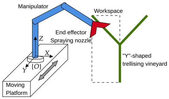
The robotic manipulator consists of a serial manipulator with prismatic (P) and revolute (R) joints. It has six degrees of freedom (DOFs) in the joint space ($n=6$). Consequently, the manipulator has six DOFs in the workspace ($m=6$). The first three DOFs correspond to the positioning mechanism that aims at positioning the wrist center in the Cartesian space. In contrast, the last three joints, corresponding to a spherical wrist, are responsible for the orientation of the spraying nozzle (end effector). Eight serial manipulator architectures were investigated for the positioning mechanism, namely $RRR$, $RRP$, $RPR$, $RPP$, $PRR$, $PRP$, $PPR$, and $PPP$ positioning structures combined with a spherical wrist. Moreover, the manipulator is considered to be mounted on a moving platform attached to the inertial frame $\left\{O\right\}$ that moves along the Y axis (see Figure 1).

Figure 1. Spraying task in vineyard: moving platform, manipulator configuration (blue); spraying nozzle (red) coupled to the end effector and rectangular workspace definition adapted to vineyard trellis geometry.

The geometric parameters of the manipulator correspond to the design variables. These design variables, $\mathbf{x}$, are derived from the Denavit–Hartenberg (DH) convention (see Appendix A) with $\mathbf{x}\in \mathbf{X}$ being $\mathbf{X}$ the design variable space. Thus, the design variables corresponding to the $i-th$ revolute links and the prismatic links are set as the vectors ${\mathbf{x}}_{Ri}=[a_i,d_i,{\alpha }_i]$ and ${\mathbf{x}}_{Pi}=[a_i,{\alpha }_i,{\theta }_i]$. Moreover, the inertia parameters are defined by the link geometry, parameterized using DH parameters.

The kinematic model of the manipulator is necessary to quantify the kinematic performance. For this end, the joint space ($\mathbf{Q}$) is defined as a joint position vector, $\mathbf{q}={\left[\begin{array}{cccc}{q}_1& q_2& \dots & q_6\end{array}\right]}^T\in \mathbf{Q}$. The first three joints can be revolute (R) or prismatic (P), depending on the manipulator architecture. The joint limits are also constrained in the following way: ${\mathbf{q}}_{min}\le \mathbf{q}\le {\mathbf{q}}_{max}$. Therefore, $\mathbf{q}\in {\mathbf{Q}}_c$ with ${\mathbf{Q}}_c$ being the constrained joint space (${\mathbf{Q}}_c\subset \mathbf{Q}$).

Moreover, the optimal design aims to optimize the manipulator’s performance to carry out the spraying task, specified by a reachable workspace in which the spraying nozzle (attached end effector) should be positioned and oriented. Therefore, the workspace inscribe the “Y”-shaped trellising vineyard [14] as presented in Figure 1). The reachable workspace ($\mathbf{W}$) is the set of coordinates that the manipulator’s end effector can reach. The manipulator’s forward kinematic model equations $\varphi (.)$ map design variables, $\mathbf{x}$, and the joint positions, $\mathbf{q}$, onto the workspace $\varphi (\mathbf{x},\mathbf{q})\to \mathbf{W}$.

In this direction, the complete pose of the end effector over the workspace is described using the homogeneous matrix, ${\mathbf{T}}_w$, that represents both rotation (orientation) and translation (position), thus: $\mathbf{T}:=\left[\begin{array}{cc}{\mathbf{R}}_w& {\mathbf{t}}_w\\ ine\mathbf{0}& 1\end{array}\right]$ where ${\mathbf{R}}_w\in {\mathbb{R}}^{3\times 3}$ is the orientation matrix and ${\mathbf{t}}_w\in {\mathbb{R}}^{3\times 1}$ is the Cartesian position with respect to the inertial frame $\left\{O\right\}$.

2.2. Design Requirements and Assumptions

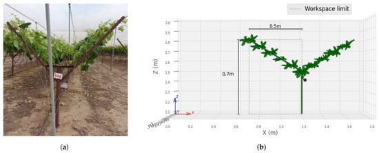
Initially, the manipulator is mounted on a platform that moves perpendicularly to the crop rows, establishing a linear degree of freedom (DOF) along the rows of vineyard with “Y”-shaped (see Y-axis of Figure 2a). The desired manipulator’s workspace ($\mathbf{w}\in \mathbf{W}$) is defined as the Cartesian positions of a rectangular space limited by the maximum and minimum positions of the grape clusters that may not be dispersed uniformly within the workspace; thus, the workspace is defined as a rectangular plane of (0.7 × 0.5) m (see Figure 2b). Then, the four corners of a rectangular plane were chosen as the extreme positions that the manipulator should reach with respect to the inertial frame $\left\{O\right\}$, which is defined with its origin located at ${\left[\begin{array}{ccc}0& 0& 1.1\end{array}\right]}^T$ m with respect to the global system (see Figure 2b).

Figure 2. The vineyard trellis infrastructure and robotic workspace simulation: (a) “Y”-shaped structure to support the grapevines [8]. (b) Simulated grapevine model and the robotic manipulator’s workspace, representing the actual task environment.

In accordance with the workspace definition and the inertial frame $\left\{O\right\}$ that define the pose of the manipulator (see Figure 2b), the first link is defined as follows to obtain feasible designs consistent: $a_0=0.0\mathrm{m}$, ${\alpha }_0={90}^{\circ }$, $d_0=0.0\mathrm{m}$ (for the revolute link) and $a_0=0\mathrm{m}$, ${\alpha }_0=-{90}^{\circ }$, ${\theta }_0=0^{\circ }$ (For prismatic joint). The design variables, $\mathbf{x}$, are defined according the DH parameters of Appendix A for the different manipulator architectures ($RRR$, $RRP$, $RPR$, $RPP$, $PRR$, $PRP$, $PPR$, and $PPP$) and the spherical wrist.

$${\mathbf{x}}_{Li}=\left\{\begin{array}{cc}\left[\begin{array}{ccc}{a}_i& d_i& {\alpha }_i\end{array}\right]\hfill & \mathrm{if}Li=R\hfill \\ \left[\begin{array}{ccc}{a}_i& {\alpha }_i& {\theta }_i\end{array}\right]\hfill & \mathrm{if}Li=P\hfill \end{array}\right.$$

(1)

Consequently, the design variables vector sets seven geometric parameters: $\mathbf{x}=\left[\begin{array}{ccc}{\mathbf{x}}_{L2}& {\mathbf{x}}_{L3}& d_6\end{array}\right]$ being ${\mathbf{x}}_{Li}$, for $i=2,3$. These geometric parameters define the second and third links, which can be revolute or prismatic. Moreover, $d_6$ corresponds to the wrist length (distance from the wrist center to the end effector).

The robotic manipulator must possess the following characteristics to execute the spraying task successfully. First, it must be capable of orienting the end effector across a wide range of angles at any given Cartesian position within the workspace. This flexibility allows the nozzle to spray grape clusters from multiple directions, ensuring thorough coverage while avoiding obstacles and foliage occlusion. Second, high kinematic dexterity is necessary to achieve precise, smoother trajectories during spraying operations. In addition, high dexterity allows the manipulator to maintain favorable configurations, effectively maximizing the distance from kinematic singularities. Finally, minimizing actuator power requirements during the motion is essential to reducing actuator effort. In agricultural robotics, energy-efficient trajectories directly increase operational productivity and significantly reduce total operational costs.

2.3. Kinematic and Dynamic Modeling

The kinematic mapping from the task space to the joint space must be established to evaluate the motion planning of the redundant system. The manipulator’s inverse kinematic equation depends on workspace position (${\mathbf{t}}_{\mathbf{w}}\in \mathbf{w}$) and the design variables ($\mathbf{x}$).

$$\mathbf{q}={\varphi }^{-1}({\mathbf{t}}_{\mathbf{w}},\mathbf{x})$$

(2)

being ${\varphi }^{-1}(.)$ the inverse kinematic equations. The inverse kinematics of Equation (2) conveys multiple solutions for the joint positions $\mathbf{q}$. The inverse kinematics solution in Equation (2) determines only the end-effector position; because the orientation is unconstrained, multiple solutions can be obtained for a single Cartesian position ${\mathbf{t}}_{\mathbf{w}}$. In this direction, the workspace DOFs ($m=3$) are less than the joint space DOFs ($n=6$). The primary objective aims to determine the joint vector $\mathbf{q}$ for a given set of design variables $\mathbf{x}$ such that the manipulator configuration maximizes its distance from the joint limits.

The Jacobian matrix, $\mathbf{J}(\mathbf{q},\mathbf{x})$, is defined as the differential mapping that relates the joint space velocities $\dot{\mathbf{q}}$ to the end-effector linear and angular velocities ${\left[\begin{array}{cc}\dot{\mathbf{t}}& \omega \end{array}\right]}^T$ in the task space, expressed as follows:

$${\left[\begin{array}{cc}\dot{\mathbf{t}}& \omega \end{array}\right]}^T=\mathbf{J}(\mathbf{q},\mathbf{x})\dot{\mathbf{q}},$$

(3)

where $\mathbf{J}(\mathbf{q},\mathbf{x})\in {\mathbb{R}}^{6\times 6}$ is the manipulator Jacobian. It is important to note that the Jacobian matrix is configuration-dependent, relying explicitly on both the joint pose $\mathbf{q}$ and the design variables $\mathbf{x}$.

The serial manipulator is kinematically decoupled, with the first three DOFs corresponding to positioning and the last three to orientation (spherical wrist) [23]. The Jacobian matrix of Equation (3) can be expressed in a block structure that separates position and orientation contributions

$$\mathbf{J}(\mathbf{x},\mathbf{q})=\left[\begin{array}{cc}{\mathbf{J}}_t& \mathbf{0}\\ {\mathbf{J}}_{\omega ,1}& {\mathbf{J}}_R\end{array}\right],$$

(4)

where ${\mathbf{J}}_t(\in {\mathbb{R}}^{3\times 3}$ is the position Jacobian associated with the first three joints, ${\mathbf{J}}_R\in {\mathbb{R}}^{3\times 3}$ is the orientation Jacobian of the spherical wrist and ${\mathbf{J}}_{\omega ,1}\in {\mathbb{R}}^{3\times 3}$ represents the contribution of the first three joints to the angular velocity of the end effector.

The position Jacobian matrix ${\mathbf{J}}_t$ of Equation (4) presents dimensional inconsistency when both revolute and prismatic joints are considered. In particular, columns associated with revolute joints have units of length, whereas those associated with prismatic joints are dimensionless [24]. A normalized Jacobian matrix to ensure dimensional homogeneity is defined as:

$${\tilde{\mathbf{J}}}_t={\mathbf{J}}_t\mathbf{D},$$

(5)

where $\mathbf{D}=\mathrm{diag}(s_1,s_2,s_3)$ is a scaling matrix defined as follows:

$$s_i=\left\{\begin{array}{cc}{\displaystyle \frac{1}{L_{ci}\left(\mathbf{x}\right)}},\hfill & \mathrm{if}\mathrm{joint}i\mathrm{is}\mathrm{revolute},\hfill \\ 1,\hfill & \mathrm{if}\mathrm{joint}i\mathrm{is}\mathrm{prismatic}.\hfill \end{array}\right.$$

This parameterization dynamically updates $L_{ci}$ during optimization to ensure dimensionally consistent evaluations across different manipulator architectures. The characteristic length $L_{ci}\left(\mathbf{x}\right)$ is dynamically parameterized according to the dimensions of the design variables vector $\mathbf{x}$. For revolute joints, $L_{ci}\left(\mathbf{x}\right)=\sqrt{a_i^2+d_i^2}$, where $a_i$ and $d_i$ represent the D-H parameters of $i-th$ link according Equation (1). For prismatic joints, $s_i=1$ (units of ${\mathrm{m}}^{-1}$ or dimensionless, since linear joint displacements naturally match workspace dimensions. This normalization allows the use of performance indices such as the condition number and manipulability in a dimensionally consistent manner.

Finally, the inverse dynamics equation of an n-joint serial manipulator can be expressed as follows:

$$\tau \left(t\right)=\mathit{M}\left(\mathbf{q}\left(t\right)\right)\ddot{\mathbf{q}}\left(t\right)+\mathit{C}(\mathbf{q}\left(t\right),\dot{\mathbf{q}}\left(t\right))\dot{\mathbf{q}}\left(t\right)+\mathit{g}\left(\mathbf{q}\left(t\right)\right)$$

(6)

were $\tau \left(t\right)\in {\mathbb{R}}^n$ is the joint torque vector, $\mathit{M}\left(\mathbf{q}\left(t\right)\right)\in {\mathbb{R}}^{n\times n}$ is the inertia matrix, $\mathbf{q}\left(t\right)\in {\mathbb{R}}^n$ is the joint position vector, $\dot{\mathbf{q}}\left(t\right)$ and $\ddot{\mathbf{q}}\left(t\right)$ are joint velocity and acceleration, $\mathit{C}(\mathbf{q}\left(t\right),\dot{\mathbf{q}}\left(t\right))\in {\mathbb{R}}^{n\times n}$ is the Coriolis and centrifugal matrix and $\mathit{g}\left(\mathbf{q}\left(t\right)\right)\in {\mathbb{R}}^n$ is the gravity vector.

2.4. Design Criteria

This subsection introduces the posture assessment approach, followed by the formulation of two objective functions derived from the kinematic and dynamic model.

2.4.1. Reachability and Posture Assessment Definitions

The inverse kinematic equation of Equation (2) yields multiple solutions because only the Cartesian position of the end effector is specified. Therefore, it is necessary to obtain the joint position $\mathbf{q}$ that maximizes the reachability, which determines the joint performance of the manipulator, i.e., the reachability indicates how close the joint position solution is to the mid-range of joint limits defined by $\mathbf{q}\in {\mathbf{Q}}_c$. This condition permits expressing how the joints are defined in the mid-range of ${\mathbf{Q}}_c$, considering a fixed Cartesian position within the workspace ${\mathbf{t}}_{\mathbf{w}}\in \mathbf{w}$.

The inverse kinematic equation is numerically solved based on the Levenberg-Marquardt method [25]. Considering a initial random position ${\mathbf{q}}_0(\Omega )\sim \mathcal{U}({\mathbf{q}}_{min},{\mathbf{q}}_{max})$ with $\mathcal{U}({\mathbf{q}}_{min},{\mathbf{q}}_{max})$ being a uniform distribution function and $\Omega$ represents all possible outcomes of the sampling space. Thus, the inverse kinematic equation is

$$\mathbf{q}(\Omega )={\varphi }^{-1}({\mathbf{t}}_w,{\mathbf{q}}_0(\Omega )).$$

(7)

The Monte Carlo Simulation (MCS) method is used to evaluate the expression of Equation (7) with the two following steps: $\left(i\right)$ the random initial joints ${\mathbf{q}}_{0s}(\Omega )$ are sampled to obtain a set of $n_s$ random inputs ${\mathbf{Q}}_{0s}={\left\{{\mathbf{q}}_0^{\left(i\right)}\right\}}_{i=1}^{n_s}$ with ${\mathbf{q}}_0\in {\mathbb{R}}^{n_s\times n}$. $\left(ii\right)$ the joint position set is obtained by solving the inverse kinematics of Equation (7) for each random input ${\mathbf{Q}}_{0s}$; thus, ${\mathbf{Q}}_s={\left\{{\mathbf{q}}^{\left(i\right)}\right\}}_{i=1}^{n_s}$ is obtained.

The following expression quantify the reachability ($RI$ for an obtained joint position ${\mathbf{q}}^{\left(i\right)}$:

$$R{I}^{\left(i\right)}=\underset{q_j}{\min }{\left({\displaystyle \frac{(q_{j,max}-q_j)(q_j-q_{j,min})}{{\left(0.5(q_{j,max}-q_{j,min})\right)}^2}}\right)}_{j=1}^{n=6}$$

(8)

being $j=1,\dots ,6$ the joint element of a given ${\mathbf{q}}^{\left(i\right)}=[q_1^{\left(i\right)},\dots ,q_j^{\left(i\right)},\dots ,q_6^{\left(i\right)}]$. When the inverse kinematic of Equation (7) has at least one solution: $R{I}^{\left(i\right)}\in [0,1]$. $R{I}^{\left(i\right)}=$ 0 when at least one of the joints is at its extreme position. $R{I}^{\left(i\right)}=1$ is the best solution, indicating that all joints are defined at mid-range. Therefore, increase the joint performance of the implies to obtain ${\mathbf{q}}^{\left(i\right)}$ that maximizes $R{I}^{\left(i\right)}$. Thus, it is considered the maximum reachability among all $\left(i\right)$ samples: $RI={\max }_{{\mathbf{q}}^{\left(i\right)}}R{I}^{\left(i\right)}$ according to Algorithm 1.

The posture index ($PI$) measures the manipulator’s capability to obtain a wide range of joint space solutions by evaluating the extreme solutions obtained among the set of $n_s$ obtained joint positions defined by the elements of ${\mathbf{Q}}_s=[{\mathbf{q}}^{\left(1\right)},\dots ,{\mathbf{q}}^{\left(n_s\right)}]$ obtained from (7). Thus, the posture index is

$$PI=mean\left({\displaystyle \frac{\max \left({\mathbf{Q}}_s\right)-\min \left({\mathbf{Q}}_s\right)}{{\mathbf{q}}_{max}-{\mathbf{q}}_{min}}}\right)$$

(9)

Thus, $PI\in [0,1]$. $P{I}^{\left(i\right)}=1$ indicates that the manipulator is capable of positioning its end effector at the position ${\mathbf{t}}_{\mathbf{w}}$ with the range of all possible joints (over all the constrained joint space (${\mathbf{Q}}_c$). $R{I}^{\left(i\right)}$ close to zero indicates a limited joint range for a specific end-effector Cartesian position. The posture index quantifies the capability for obstacle avoidance, and it also indicates the range of multiple orientations available for the end effector, considering a specific definition of the design parameters ($\mathbf{x}$) and Cartesian position (${\mathbf{t}}_{\mathbf{w}}$). The last part of Algorithm 1 shows the procedure to compute $PI$.

Finally, the reachability index ($RI$) evaluates the joint vector $\mathbf{q}$ to prevent configurations from approaching their physical joint limits.

To quantify the impact ot the posture index ($PI$) on the nozzle’s directional flexibility for canopy penetration, the dispersion angle ${\Delta }_{\theta }$ was formulated as the mean of the pairwise angular distances between viable nozzle orientations corresponding to the joint boundary joint positions used to compute $PI$ in Equation (9) ($\min \left({\mathbf{Q}}_s\right)$ and $\max \left({\mathbf{Q}}_s\right)$) and the middle joint position ($\mathrm{mean}\left({\mathbf{Q}}_s\right)$). Forward kinematics map the boundary and mean joint positions into corresponding unit quaternions (${\mathbf{u}}_k\in S^3$ for $k=1,2,3$) [25]. The geodesic distances on $S^3$ between the corresponding relative quaternion is defined as ${\theta }_{ij}=angvec({\mathbf{u}}_i^{-1}\otimes {\mathbf{u}}_j)$. Thus, the dispersion angle ${\Delta }_{\theta }$ corresponds to the average of quaternions’ geodesic distances as presented in Equation (10).

$${\Delta }_{\theta }={\displaystyle \frac{({\theta }_{\max ,\min }+{\theta }_{\max ,\mathrm{mean}}+{\theta }_{\min ,\mathrm{mean}})}{3}}$$

(10)

Algorithm 1 Algorithm that describes how to compute the reachability index ($RI$) and posture index ($PI$).
1: Function reachability and posture($\mathbf{x}$, ${\mathbf{t}}_{\mathbf{w}}$, ${\mathbf{q}}_{min}$, ${\mathbf{q}}_{max}$, $n_s$)
2: ${\mathbf{Q}}_s\leftarrow \left[\right]$, $\mathbf{RI}\leftarrow \left[\right]$
3: for  $i=1$  to  $n_s$  do
4:        ${\mathbf{q}}_0^{\left(i\right)}\leftarrow \mathrm{random}\_\mathrm{sample}({\mathbf{q}}_{min},{\mathbf{q}}_{max})$	▹ Sampling of: $\mathcal{U}({\mathbf{q}}_{min},{\mathbf{q}}_{max})$
5:        ${\mathbf{q}}^{\left(i\right)}\leftarrow {\varphi }^{-1}({\mathbf{t}}_{\mathbf{w}},{\mathbf{q}}_0^{\left(i\right)})$	▹ Inverse kinematic solution
6:        $R{I}^{\left(i\right)}\leftarrow \min \left({\displaystyle \frac{({\mathbf{q}}_{max}-{\mathbf{q}}^{\left(i\right)})({\mathbf{q}}^{\left(i\right)}-{\mathbf{q}}_{min})}{{\left(0.5({\mathbf{q}}_{max}-{\mathbf{q}}_{min})\right)}^2}}\right)$	▹ From Equation (8)
7:        ${\mathbf{Q}}_s\leftarrow solutions\cup \left\{{\mathbf{q}}^{\left(i\right)}\right\}$
8:        $\mathbf{RI}\leftarrow solutions\cup \left\{R{I}^{\left(i\right)}\right\}$
9: end for
10: $PI\leftarrow mean\left({\displaystyle \frac{max\left({\mathbf{Q}}_s\right)-\min \left({\mathbf{Q}}_s\right)}{{\mathbf{q}}_{max}-{\mathbf{q}}_{min}}}\right)$	▹ From Equation (9)
11: $idx\leftarrow \arg \max \left(\mathbf{RI}\right)$
12: return  ${\mathbf{Q}}_s\left[idx\right],\mathbf{RI}\left[idx\right],PI$

The specific joint position $\mathbf{q}$ that maximizes this reachability is subsequently used to compute the global conditioning index ($GCI$), as detailed in the following section.

2.4.2. Global Conditioning Index

The Global Conditioning Index ($GCI$) is a widely adopted metric for assessing kinematic dexterity [26]. This index relies on the reciprocal of the condition number of the normalized position Jacobian matrix of Equation (5), $1/\kappa \left({\tilde{\mathbf{J}}}_{\mathbf{t}}(\mathbf{x},\mathbf{q})\right)$, to quantify local maneuverability. This value ranges from 0, representing a singular configuration, to 1, representing an isotropic state. Within the desired workspace $\mathbf{w}$, thus $\mathbf{q}\in {\varphi }^{-1}({\mathbf{t}}_{\mathbf{w}},\mathbf{x})\forall {\mathbf{t}}_{\mathbf{w}}\in \mathbf{w}$. It worth to say that $\mathbf{q}$ is computed using Algorithm 1.

$$GCI(\mathbf{x},\mathbf{q})={\displaystyle \frac{{\int }_{\mathbf{w}}1/\kappa \left({\tilde{\mathbf{J}}}_{\mathbf{t}}(\mathbf{x},\mathbf{q})\right)d\mathbf{w}}{{\int }_{\mathbf{w}}d\mathbf{w}}}$$

(11)

Because a higher $GCI$ value correlates with superior kinematic performance across the workspace, the index is typically treated as an objective function to be maximized during the design.

The Posture Index ($PI$) of Equation (9) evaluates the posture at a single posture. Consequently, the Global Posture Index ($GPI$) is also proposed to evaluate posture within the desired workspace.

$$GPI(\mathbf{x},\mathbf{q})={\displaystyle \frac{{\int }_{\mathbf{w}}PId\mathbf{w}}{{\int }_{\mathbf{w}}d\mathbf{w}}}$$

(12)

2.4.3. Root Mean Square (RMS) Power of Actuators

The Root Mean Square (RMS) power is calculated to account for the actuator power constraints of the actuators based on the dynamic equation of the manipulator in Equation (6). The RMS power ($P_{RMS}$) for a joint over a motion cycle of duration $t\in T$ is defined as follows:

$$P_{RMS}=\sqrt{{\displaystyle \frac{1}{T}}{\int }_0^T{\left({\tau }^T\left(t\right)\dot{\mathbf{q}}\left(t\right)\right)}^{2}dt}$$

(13)

The instantaneous mechanical power $\left({\tau }^T\left(t\right)\dot{\mathbf{q}}\left(t\right)\right)$ is squared prior to integration according. This accounts for negative power (occurring during regenerative deceleration or gravity-assisted motion) with the same magnitude of positive power. Consequently, the $P_{RMS}$ metric provides the actuator’s mechanical demand, which characterizes mechanical effort. Consequently, power efficiency is improved by minimizing $P_{RMS}$.

2.5. Multi-Objective Optimization Design

The objective functions considered to optimize the manipulator performance, i.e., maximize the global conditioning index of Equation (11) to improve the kinematic dexterity ($\max f_1\left(\mathbf{x}\right)=GCI$) and minimize the actuator power requirements quantified by the root mean square of the actuator’s power defined in Equation (13) ($\min f_2\left(\mathbf{x}\right)=P_{RMS}$), simultaneously. The following parameters are defined based on physical constraints, such as material properties and maximum link lengths, and are incorporated directly into the optimization method.

The bounds of design variables $\mathbf{x}$ are defined according to the geometrical feasibility of the link’s lengths and angles following the DH convention of Equation (1). For revolute joints, the limits are defined as ${\mathbf{x}}_{Ri}^{\min }={\left[\begin{array}{ccc}0\mathrm{m}& 0\mathrm{m}& 0^{\circ }\end{array}\right]}^T$ and ${\mathbf{x}}_{Ri}^{\max }={\left[\begin{array}{ccc}1\mathrm{m}& 1\mathrm{m}& {180}^{\circ }\end{array}\right]}^T$. Conversely, for prismatic joints, the bounds are ${\mathbf{x}}_{Pi}^{\min }={\left[\begin{array}{ccc}0\mathrm{m}& -{180}^{\circ }& -{180}^{\circ }\end{array}\right]}^T$ and ${\mathbf{x}}_{Pi}^{\max }={\left[\begin{array}{ccc}1\mathrm{m}& 0^{\circ }& 0^{\circ }\end{array}\right]}^T$. Finally, the wrist length is constrained by $d_6^{\min }=0\mathrm{m}$ and $d_6^{\max }=1\mathrm{m}$. Furthermore, the joint limits for the present application are defined as $-{180}^{\circ }\le q_i\le {180}^{\circ }$ for revolute joints and 0 m $\le q_i\le 0.9$ m for prismatic joints. According to Algorithm 1, the number of samples ($n_s$) required to evaluate the inverse kinematics to compute the posture index ($PI$) was defined as $n_s=70$; this definition produces an output variation less than 7%.

The linear mass density of the links was considered as $1.5\mathrm{kg}/\mathrm{m}$, which corresponds to an aluminum tube with 60 mm outer diameter and a 3 mm thickness. Additionally, the actuators are modeled as base-mounted, massless elements relative to the moving structure. Mounting the actuators directly to the stationary base isolates their physical mass from the moving kinematic chain, eliminating their contribution to the manipulator’s inertia matrix $\mathbf{M}\left(\mathbf{q}\right)$ and Coriolis/centrifugal terms $\mathbf{C}(\mathbf{q},\dot{\mathbf{q}})$. Motion and torque are transmitted to the distal links via lightweight, high-tensile steel cables and aluminum push rods. Consequently, the omission of these dynamic effects on joint torques is justified to maintain computational efficiency during multi-objective design optimization. An agricultural spray nozzle assembly was modeled with a mass of $m_{\mathrm{nozzle}}=0.10\mathrm{kg}$, corresponding to lightweight plastic/brass agricultural spray, whose mass and inertia are less than 5% compared with the average link masses ($m_{link}=2.0\mathrm{kg}$); its dynamic contribution is dominated by the link’s inertia of the manipulator.

The motion consists of a joint space between the initial joint position ${\mathbf{q}}_0=[{\mathbf{q}}_{0t},{\mathbf{q}}_{0R}]$ and final joint position ${\mathbf{q}}_f=[{\mathbf{q}}_{ft},{\mathbf{q}}_{fR}]$ for the actuators’ power based on the dynamic model of Equation (13). The joint trajectory was interpolated with a fifth-order polynomial with rest-to-rest boundary conditions; the trajectory duration $T=5.0\mathrm{s}$ was standardized for all trajectories to evaluate RMS power ($P_{\mathrm{RMS}}$). For the eight manipulator architectures, the position boundary conditions for the first three joints (${\mathbf{q}}_{0t}$ and ${\mathbf{q}}_{ft}$) were set based on whether each joint was revolute ($R_i$) or prismatic ($P_i$) for $i=1,2,3$. Revolute joint boundaries were defined as $q_{0,R_1}=-5.0^{\circ }$ to $q_{f,R_1}=5.0^{\circ }$, $q_{0,R_2}=0.0^{\circ }$ to $q_{f,R_2}=45.0^{\circ }$, and $q_{0,R_3}=90.0^{\circ }$ to $q_{f,R_3}=180.0^{\circ }$. For prismatic joints, the boundaries were set to $q_{0,P_1}=0.00\mathrm{m}$ to $q_{f,P_1}=0.45\mathrm{m}$, $q_{0,P_2}=0.15\mathrm{m}$ to $q_{f,P_2}=0.00\mathrm{m}$, and $q_{0,P_3}=0.80\mathrm{m}$ to $q_{f,P_3}=0.10\mathrm{m}$. Moreover, the wrist orientation boundaries remained identical for all architectures, transitioning from ${\mathbf{q}}_{0R}={[0^{\circ },-{45}^{\circ },-{45}^{\circ }]}^T$ to ${\mathbf{q}}_{fR}={[{45}^{\circ },0^{\circ },{45}^{\circ }]}^T$.

Moreover, a discrete $3\times 3$ sampling grid ($N_{\mathrm{total}}=9$ target points) was established to evaluate global kinematic metrics within the rectangular workspace. The grid resolution yielded less than a 5% variation in the global metrics ($GCI$ and $GPI$), while increasing the grid resolution beyond 9 points significantly increased computational cost during objective function evaluation.

The inequality constraints $g_i\left(\mathbf{x}\right)$ for $i=1,2$ were defined according to the global posture index ($GPI$ of Equation (12)) and the covered workspace considered to compute the global indices. Specifically, the first constraint, a maximum global posture index ($GP{I}_{max}$), is considered $g_1\left(\mathbf{x}\right)=GPI\left(\mathbf{x}\right)-GP{I}_{max}$ to enforce a maximum allowable global posture index ($GP{I}_{\max }$) that filters designs with differing posture characteristics. Unbounded optimization can lead to oversized link dimensions that increase robot mass and actuator power consumption with diminishing returns on task dexterity. Consequently, the constraint $GP{I}_{\max }$ allows the optimization process to filter candidate designs to determine a practical trade-off between posture quality and actuator power requirements.

The second constraint, $g_2\left(\mathbf{x}\right)=\mathbf{w}-\mathbf{w}\left(\mathbf{x}\right)$, ensures that the workspace covered by the specific design variables, denoted as $\mathbf{w}\left(\mathbf{x}\right)$, is sufficient to compute the global conditioning index ($GCI$) of Equation (11).

$$\begin{array}{cc}\hfill \underset{\mathbf{x}}{\max }& f_1\left(\mathbf{x}\right)\hfill \end{array}$$

(14)

$$\begin{array}{cc}\hfill \underset{\mathbf{x}}{\min }& f_2\left(\mathbf{x}\right)\hfill \end{array}$$

(15)

$$\begin{array}{cc}\hfill \mathrm{subject}\mathrm{to}:& {\mathbf{x}}^{\min }\le \mathbf{x}\le {\mathbf{x}}^{\max }\hfill \end{array}$$

(16)

$$\begin{array}{cc}\hfill & g_1\left(\mathbf{x}\right)\le 0\hfill \end{array}$$

(17)

$$\begin{array}{cc}\hfill & g_2\left(\mathbf{x}\right)\le 0\hfill \end{array}$$

(18)

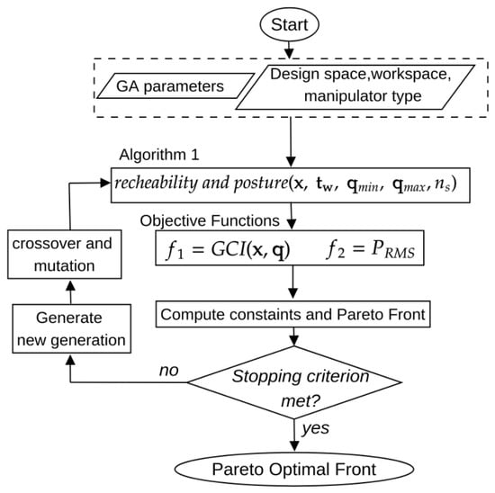
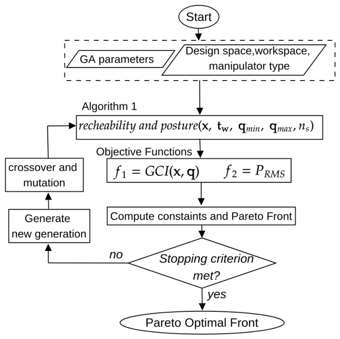
Finally, the algorithm for computing the manipulator’s geometric parameters is presented in the flowchart in Figure 3. The optimization of the manipulator of Equations (14)–(18) is solved using the NSGA-II algorithm to a set of optimal solutions denominated the Pareto front [13]. Initially, a set of candidate solutions is randomly defined within the design space of the design variables. The objective functions, namely the global conditioning indices and the RMS of the torques along a specified motion, are evaluated for these candidate solutions to generate the Pareto front, until the stopping criteria are met, following the iterative application of genetic algorithm operations (crossover and mutation).

Figure 3. Flowchart of the multi-objective optimization to compute the set of optimal design variables to define the geometry of the manipulator.

The robot model (Section 2.3) and the design criteria (Section 2.4) were implemented in Python 3.8.10 using the robotics toolbox for Python [25]. Moreover, the multi-objective optimization (MOO) problem of Equations (14)–(18) and Figure 3 was solved using Pymoo toolbox [27]. Specifically, the NSGA-II [28] algorithm was used to solve the MOO. Moreover, the algorithm was programmed in Python. The numerical simulations were performed on a system running Ubuntu 20.04 with an Intel Core i7 processor with 16GB of RAM. A parallelized multiprocessing framework was implemented to minimize computation time and maximize efficiency during inverse kinematics resolution. Independent inverse kinematics tasks are distributed across a processing pool utilizing six concurrent workers via Python’s multiprocessing module instead of executing the $n_s$ random initialization attempts sequentially according to Appendix A.

Three multi-objective (MOO) evolutionary algorithms, namely NSGA-II, C-TAEA, and SPEA2, were employed to solve the proposed constrained multi-objective optimization problem of Equations (14)–(18) using the methodology presented in the flowchart of Figure 3. The following hyperparameter configuration for the MOO algorithms was defined after preliminary experiments showed stable convergence across all evaluated field geometries, thereby establishing a reliable basis for comparative analysis. A uniform population of 150 individuals was set, and the algorithms ran for 100 generations. The search space was explored using the Simulated Binary Crossover (SBX) operator with a crossover probability of 0.9 and a distribution index of 25 to preserve population diversity.

3. Results

3.1. Reachability and Posture Assessment

This analysis illustrates how the joint-coordinate ranges translate into achievable ranges of nozzle orientation. The posture index ($PI$) of Equation (9) was evaluated across three manipulator architectures ($RRR$, $RPP$ and $PPP$) for three representative joint configurations $\max \left({\mathbf{Q}}_s\right)$ (posture 1), $\min \left({\mathbf{Q}}_s\right)$ (posture 2) and $mean\left({\mathbf{Q}}_s\right)$ (posture 3 that is indeterminate). The posture index ($PI$) was analyzed for three different nozzle Cartesian positions ${\mathbf{t}}_{wi}$ with $i=1,2,3$. The design variables of the corresponding manipulator architectures were defined as ${\mathbf{x}}_{RRR}=\left[\begin{array}{c}0.44\mathrm{m},0.99\mathrm{m},{101}^{\circ },0.86\mathrm{m},0.17\mathrm{m},4.{32}^{\circ },0.09\mathrm{m}\end{array}\right]$, ${\mathbf{x}}_{RPP}=\left[\begin{array}{c}0.44\mathrm{m},0.{99}^{\circ },{101}^{\circ },0.86\mathrm{m},0.{17}^{\circ },4.{32}^{\circ },0.09\mathrm{m}\end{array}\right]$ and ${\mathbf{x}}_{PPP}=\left[\begin{array}{c}0\mathrm{m},-90.0^{\circ },-90.0^{\circ },0\mathrm{m},-43.{20}^{\circ },-117.{67}^{\circ },0.31\mathrm{m}\end{array}\right]$.

Consequently, the nozzle’s orientation reachability was evaluated using the mean angular dispersion (${\Delta }_{\theta }$) according to Equation (10), which expresses the directional range of the nozzle associated with a given posture index ($PI$). The results indicate a strong correlation between a higher posture index $\left(PI\right)$ and a wider nozzle orientation range, as presented in Table 1. Among the evaluated manipulator architectures, the $RRR$ architecture consistently achieves superior posture outputs, whereas architectures with joints ($RPP$ and $PPP$) exhibit degraded performance. Minor non-linearities between $PI$ and ${\Delta }_{\theta }$ (such as $RRR$ at ${\mathbf{t}}_{w2}$) mean that the manipulator prioritizes the tree initial joints responsible for positioning over wrist rotation. This separation is ideal for vineyard spraying, as the manipulator can maneuver around dense foliage while keeping the nozzle properly aimed.

Table 1. Comparative posture index ($PI$) assessment considering the manipulator architectures $RRR$ + wrist, $RPP$ + wrist, and $PPP$ + wrist for three different postures.

	RRR		RPP		PPP
	$\mathit{P}\mathit{I}$	Δθ(°)	$\mathit{P}\mathit{I}$	Δθ(°)	$\mathit{P}\mathit{I}$	Δθ(°)
${\mathbf{t}}_{w1}^{*}$	0.91	108.75	0.77	111.93	0.64	69.46
${\mathbf{t}}_{w2}^{*}$	0.90	150.54	0.71	126.54	0.55	126.02
${\mathbf{t}}_{w3}^{*}$	0.96	124.34	0.51	101.72	0.12	30.49

* Cartesian positions of end effector: ${\mathbf{t}}_{w1}=\left[\begin{array}{ccc}0.7& 0.0& 1.8\end{array}\right]$ m, ${\mathbf{t}}_{w2}=\left[\begin{array}{ccc}0.9& 0.0& 1.6\end{array}\right]$ m and ${\mathbf{t}}_{w3}=\left[\begin{array}{ccc}1.2& 0.0& 1.1\end{array}\right]$ m.

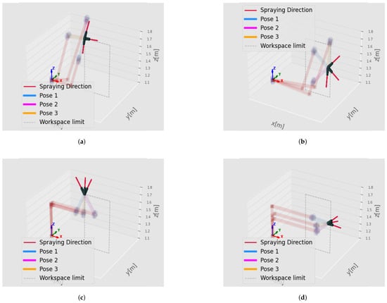
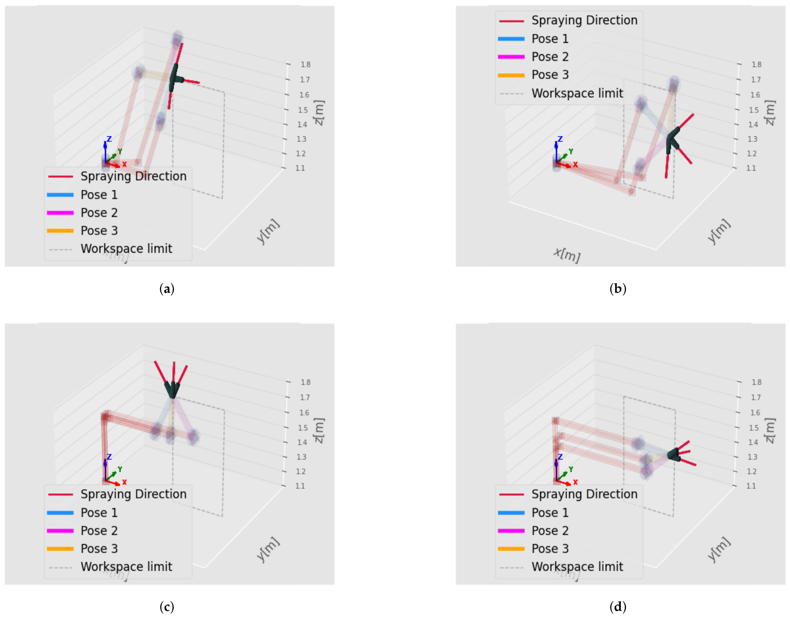
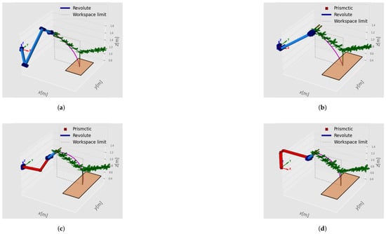
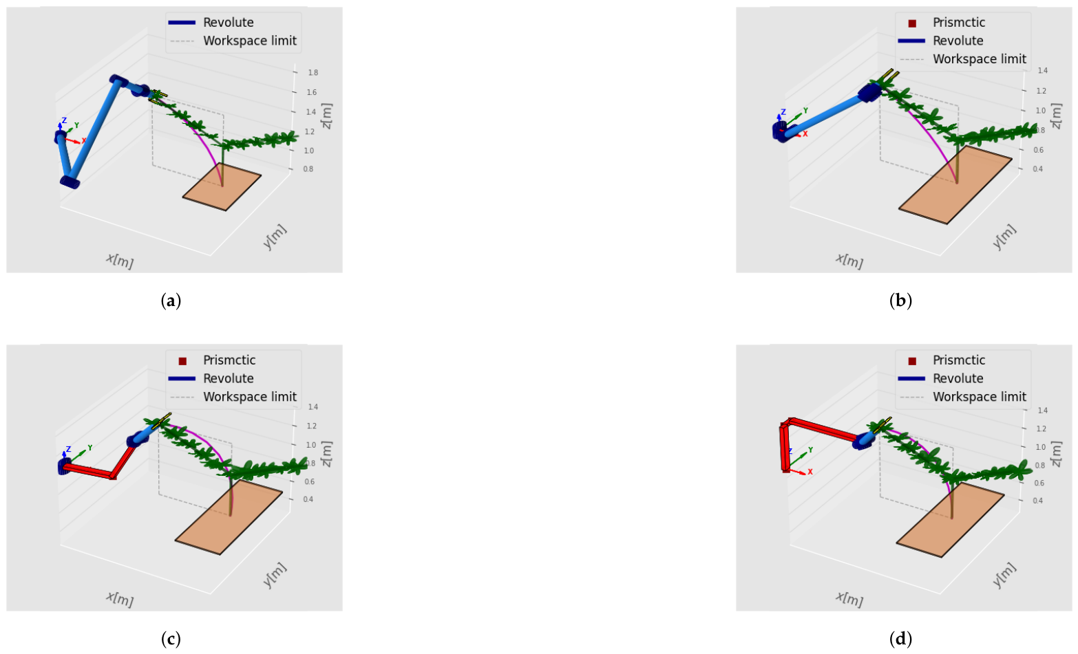
The nozzle’s orientation is illustrated in Figure 4 considering the $RPP$ + wrist manipulator at the positions ${\mathbf{t}}_{w1}$ (see Figure 4a) and ${\mathbf{t}}_{w3}$ (see Figure 4b). As the prismatic joints extend to lower, deeper points in the workspace, the joint limits constrain the remaining movement range, reducing ${\Delta }_{\theta }$. This restricts the nozzle’s orientation, making it harder to position it effectively. Additionally, a reduced angular dispersion ${\Delta }_{\theta }$ is observed for the $PPP$ + wrist manipulator evaluated at position ${\mathbf{t}}_{w1}$ (see Figure 4c) and position position ${\mathbf{t}}_{w3}$ (see Figure 4d).

Figure 4. Nozzle’s orientation considering two different target positions: (a) $RPP$ + wrist manipulator at ${\mathbf{t}}_{w1}$. (b) $RPP$ + wrist manipulator at ${\mathbf{t}}_{w3}$. (c) $PPP$ + wrist manipulator at ${\mathbf{t}}_{w1}$. (d) $PPP$ + wrist manipulator at ${\mathbf{t}}_{w3}$.

3.2. Multi-Objective Design

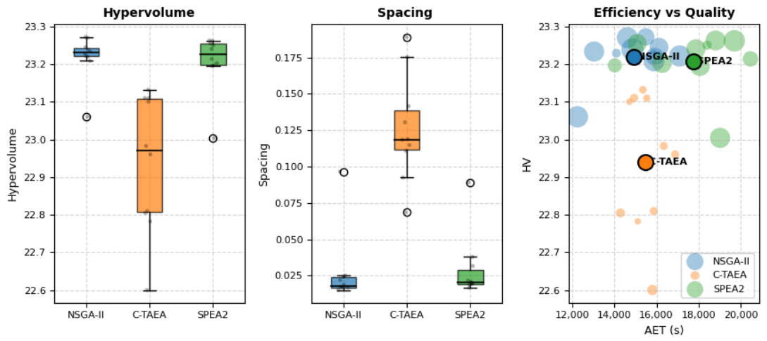
Initially, the multi-objective optimization problem of Equations (14)–(18) was solved to evaluate the performance of three evolutionary algorithms (NSGA-II, C-TAEA, and SPEA2) across eight distinct manipulator architectures ($RRR$ through $PPP$). A uniform configuration of 100 generations and a population size of 150 individuals was used across all algorithms to ensure a fair comparison. Three specific metrics were utilized to evaluate solution quality alongside computational efficiency: average execution time (AET), Hypervolume (HV), and Spacing.

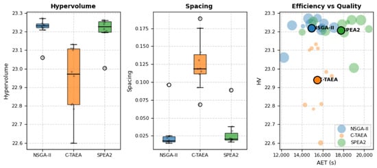
Initially, 10 independent runs were conducted for NSGA-II, C-TAEA, and SPEA2 to evaluate the multi-objective evolutionary algorithms for optimizing the $RRR$ robot manipulator, and their corresponding outputs are presented in Figure 5. NSGA-II established clear dominance over C-TAEA and SPEA2 because it simultaneously maximized solution quality, obtaining the highest HV, ensured superior trade-off diversity (lowest and most stable Spacing); Moreover, NSGA-II minimized computational burden (lowest AET). Consequently, NSGA-II is selected as the primary optimization engine for evaluating the kinematic and dynamic trade-offs of the candidate manipulator architectures.

Figure 5. Comparative Performance across Optimization Algorithms and Manipulator Architectures with Summary Statistics. Computational performance evaluation of NSGA-II, C-TAEA, and SPEA2: Hypervolume (HV) indicator for convergence and diversity; Spacing (SP) metric for Pareto front distribution uniformity; and total execution time in seconds (AET).

The comparative analysis reveals a clear trade-off between computational overhead and Pareto front quality, validating NSGA-II as the superior choice for this optimization framework as detailed in Table 2. While SPEA2 consistently delivers high-quality convergence and uniform solution spread, it incurs a severe computational penalty, with execution times reaching up to 40,662.11 s. Conversely, C-TAEA offers significant computational advantages in prismatic-heavy architectures such as the $PPR$ configuration, but suffers from volatile solution spacing and reduced Hypervolume values. Ultimately, NSGA-II demonstrates the most robust performance, showing a remarkable balance by consistently producing high hypervolume metrics, low and stable spacing values, and moderate execution times across all manipulator architectures.

Table 2. Comparative Performance and Computational Effort of NSGA-II, C-TAEA, and SPEA2 algorithms considering the manipulator architectures.

	NSGA-II			C-TAEA			SPEA2
	AET (s)	HV	Spacing	AET (s)	HV	Spacing	AET (s)	HV	Spacing
$RRR$ *	12,252.17	23.06	0.0169	15,542.92	23.10	0.1415	16,262.82	23.20	0.0204
$RRP$	12,815.28	21.27	0.1188	11,945.03	19.45	0.3843	16,034.54	21.06	0.0829
$RPR$	9697.74	21.74	0.0268	4957.10	19.87	1.0662	13,040.74	21.56	0.1063
$RPP$	7575.62	22.88	0.0172	11,260.07	23.47	0.0278	12,609.05	23.32	0.0209
$PRR$	10,079.56	12.46	0.0360	4537.46	12.00	1.1270	14,828.69	12.52	0.0377
$PRP$	11,422.82	9.45	0.2545	4784.39	9.49	0.5059	13,930.97	8.90	0.1580
$PPR$	10,985.75	14.89	0.0176	2135.52	11.89	0.0	13,402.45	14.90	0.0066
$PPP$	10,287.86	18.35	0.0147	8824.80	17.70	0.2918	15,176.15	18.18	0.0059

* Manipulator architectures.

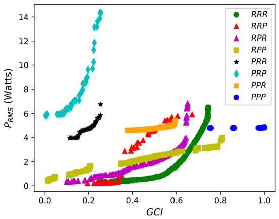
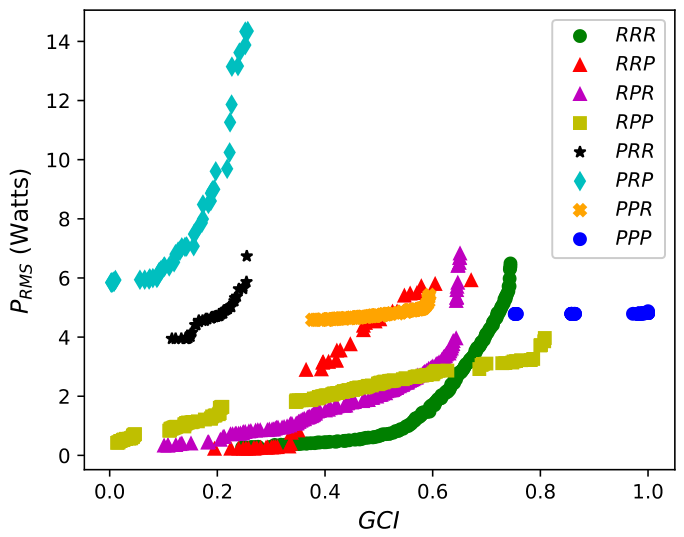
The resulting Pareto fronts for the considered manipulator architectures derived from the solution of the multi-objective optimization problem of Equations (14)–(18) using the NSGA-II algorithm are presented in Figure 6. The Pareto Fronts show the dominant solutions, i.e., the designs that optimize one objective without degrading the other. The optimization of the power of the actuator and the kinematic conditioning exhibits a concurrent behavior, i.e., the increase in the $GCI$ demands an increase in the power of the actuators ($P_{RMS}$). These Pareto fronts permit the evaluation of the set of optimal designs that simultaneously maximize the kinematic dexterity (quantified by the $GCI$ in Equation (11)) and minimize the actuator’s RMS torque.

Figure 6. Comparison of the Pareto-optimal fronts in the objective space from the solution of the multi-objective optimization (MOO) considering several architectures of manipulators: $RRR$, $RRP$, $RPR$, $RPP$, $PRR$, $PRP$, $PPR$, $PPP$.

The $RRR$ achieves high kinematic dexterity, reaching a maximum $GCI$ of approximately $0.744$, thereby ensuring high structural flexibility for dynamically reorienting spraying nozzles around dense grape foliage; nevertheless, supporting three massive rotating serial linkages induces substantial inertial loads that increase power consumption.

The $PPP$ manipulator architectures achieved the highest kinematic $GCI$ = 1 because, in their optimal configuration, the prismatic actuators are oriented orthogonally. The RMS power consumption is approximately $4.78\mathrm{W}$ to $4.87\mathrm{W}$ because their decoupled linear links minimize actuator forces.

Moreover, $RRR$, $RRP$, $RPP$, and $PPP$ manipulator architectures achieve high $GCI$, and their Pareto front solutions also show lower actuator power requirements than the $PPP$ manipulator, reconciling the concurrent objectives with well-populated Pareto fronts.

The $RRP$ and $PPR$ manipulator architectures exhibit intermediate performance (see Figure 6). They exhibit lower kinematic dexterity and higher actuator power consumption than the aforementioned manipulator architectures, i.e., they tend to be Pareto-dominated by their counterparts ($RPR$ and $RPP$).

The $PRR$ and $PRP$ architectures are classified as not suitable for the vineyard spraying operation in which the desired workspace is orthogonal to the first prismatic joint (see Figure 6). When the prismatic joint of the base is followed by a consecutive revolute joint, the inertia of the manipulator structure increases, and hence the actuator torques also increase. Therefore, these manipulator architectures yield Pareto fronts that do not simultaneously minimize actuator power consumption and ensure kinematic dexterity.

One important criterion for selecting the more appropriate manipulator design obtained from the Pareto fronts of Figure 6 is the global posture index ($GPI$) of Equation (12) that was considered within the constraint $g_1\left(\mathbf{x}\right)$ in MOO optimization (see Equation (17)). In this direction, the maximum $GPI$ of the Pareto front solutions ($max\left(GPI\right)$) was assessed to evaluate the capability of the different manipulators to orient the end effector in several directions, as presented in Table 3. One can observe that the $RRR$ and $RRP$ manipulator architectures obtained the Pareto solution that also maximizes the $GPI$ since these architectures permit positioning the spherical wrist with a wide range of orientations. The $PPP$ and $RPP$ manipulator architectures exhibit a good Pareto solution that maximizes kinematic conditioning; nevertheless, these solutions have a low posture index ($GPI$), indicating a poor capacity to orient the spherical wrist in several orientations.

Table 3. Maximum global posture index of the Pareto front of Figure 6 for the considered manipulator architectures.

	$\mathit{R}\mathit{R}\mathit{R}$	$\mathit{R}\mathit{R}\mathit{P}$	$\mathit{R}\mathit{P}\mathit{R}$	$\mathit{R}\mathit{P}\mathit{P}$	$\mathit{P}\mathit{R}\mathit{R}$	$\mathit{P}\mathit{R}\mathit{P}$	$\mathit{P}\mathit{P}\mathit{R}$	$\mathit{P}\mathit{P}\mathit{P}$
$max\left(GPI\right)$	0.7348	0.7064	0.5974	0.5464	0.6332	0.6190	0.4803	0.3752

3.3. Analysis of Global Posture Index ($GPI$) Constraint

The following analysis aims to assess the influence of the global posture index ($GPI$) as an inequality constraint in the multi-objective optimization of Equations (14)–(18) for different maximum global posture index ($GP{I}_{max}$) values. In this direction, it evaluates how the posture index constraints affect the trade-off defined by the obtained Pareto front.

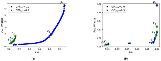
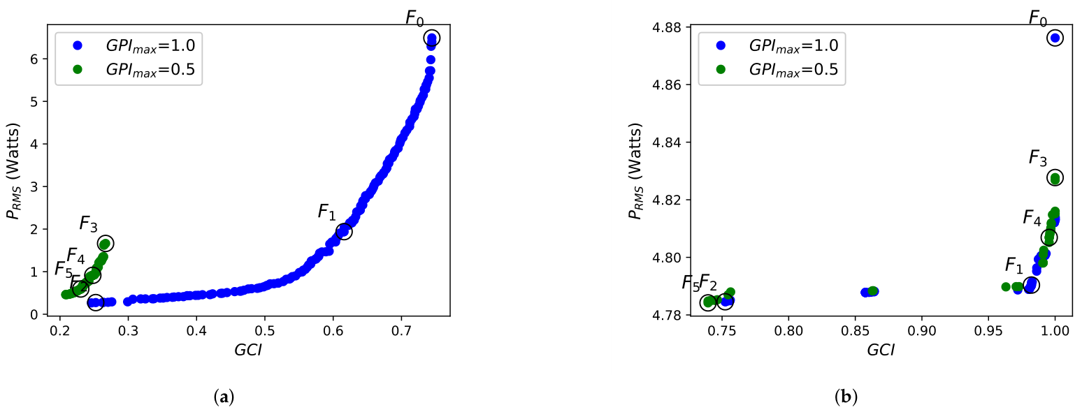
The Pareto front is presented for $RRR$ + wrist in Figure 7a and $PPP$ + wrist in Figure 7b, considering two specific valued of the global posture index ($GPI$) as a constraint ($GP{I}_{max}$ = 1.0 and $GP{I}_{max}$ = 0.5).

Figure 7. Pareto Front obtained from the solution of the MOO considering two different global posture indices ($GP{I}_{max}$): (a) $RRR$ manipulator. (b) $PPP$ manipulator.

The obtained Pareto fronts indicate that the optimal design with a higher global posture index ($GPI$) also produces manipulator designs with higher kinematic dexterity ($GCI$) for both manipulator architectures $RRR$ + wrist and $PPP$ + wrist. Therefore, higher kinematic dexterity also implies higher posture index performance, a desired characteristic for the manipulator design.

The design variables ($\mathbf{x}$) corresponding to the geometric parameters of the six selected Pareto front solutions (see Figure 7a) are shown in Table 4 of the $RRR$ + wrist manipulator. For solutions $F_0$, $F_1$, and $F_2$, the manipulator was designed under a high-posture constraint ($GP{I}_{max}=1.0$), enabling it to achieve high posture capacities ($GPI\ge 0.66$) while simultaneously achieving superior kinematic dexterity ($GCI$ up to 0.74). For solutions $F_3$, $F_4$, and $F_5$, the constraint decrease ($GP{I}_{max}=0.5$), forcing both $GPI$ and $GCI$ into lower performance. One can observe that $GPI$ does not scale linearly with $GCI$. Solution $F_1$ actually achieves the highest posture index (0.70), even though its dexterity ($GCI=0.62$) is lower than solution $F_0$ ($GCI=0.74$). This indicates a kinematic solution that is most appropriate, in which intermediate link lengths provide optimal positioning performance for the end-effector orientation without sacrificing too much kinematic dexterity in the workspace. Additionally, regarding the design variables, one can observe that larger link lengths expand the reachable workspace. However, the resulting increase in inertial mass and moment arms drastically amplifies the power required to move the robot.

Table 4. Six solutions from the Pareto Front of the $RRR$ + wrist manipulator of Figure 7a with their corresponding design variables ${\mathbf{x}}_i$ and objective functions ${\mathbf{f}}_i$ for $i=1,\dots ,5$.

${\mathit{F}}_{\mathit{i}}$ *	x							f		${\mathit{g}}_1\left(\mathbf{x}\right)$
	a2(m)	d2(m)	α2(°)	a3(m)	d3(m)	α3(°)	d6(m)	GCI	PRMS(W)	GPI
0	0.99	1.00	101.53	0.98	0.18	9.47	0.01	0.74	6.02	0.66
1	0.44	0.99	101.47	0.86	0.17	4.32	0.09	0.62	2.07	0.70
2	0.11	0.90	108.30	0.60	0.00	9.96	0.01	0.30	0.35	0.67
3	0.36	0.62	92.89	0.52	0.00	80.51	0.00	0.26	1.21	0.49
4	0.29	0.61	104.10	0.57	0.04	34.90	0.00	0.24	0.75	0.47
5	0.22	0.61	107.21	0.60	0.00	146.19	0.00	0.22	0.47	0.47

* $GP{I}_{max}$ = 1.0 for $i=0,\dots ,2$ and $GP{I}_{max}$ = 0.5. for $i=3,\dots ,5$.

The geometric parameters of the six selected solutions (see Figure 7b) are presented in Table 5 for manipulator $PPP$ + wrist considering the maximum posture index constraints ($GP{I}_{max}$ = 1.0 and $GP{I}_{max}$ = 0.5). The $PPP$ + wrist manipulator achieves an outstanding global conditioning index ($GCI=1.00$) in multiple solutions ($F_0$, $F_3$, and $F_4$) that indicate a perfectly isotropic kinematic workspace, which is a classic capability of orthogonal linear Cartesian axes. The variation in the posture index constraint has no practical effect on the robot design for the $PPP$ + wrist manipulator. The global posture index ($GPI$) remains locked within an incredibly narrow band between 0.34 and 0.39 across all six solutions, since the $PPP$ + wrist manipulator yields limited capability to orient the end effector. Solution $F_3$ represents the absolute peak of this Pareto front, as it achieves the maximum kinematic dexterity ($GCI=1.00$) while delivering the highest posture capacity ($GPI=0.39$) and maintaining a low power draw.

Table 5. Six designs from the Pareto Front of the $PPP$ + wrist manipulator of Figure 7b with their corresponding design variables ${\mathbf{x}}_i$ and objective functions ${\mathbf{f}}_i$ for $i=1,\dots ,5$.

${\mathit{F}}_{\mathit{i}}$ *	x							f		${\mathit{g}}_1\left(\mathbf{x}\right)$
	a2(m)	α2(°)	θ2(°)	a3(m)	α3(°)	θ3(°)	d6(m)	GCI	PRMS(W)	GPI
0	0.00	−90.00	−90.00	0.00	−37.59	−119.13	0.33	1.00	4.88	0.36
1	0.00	−91.03	−90.02	0.00	−53.56	−118.67	0.30	0.98	4.79	0.34
2	0.00	−91.91	−90.00	0.00	−58.07	−118.70	0.30	0.75	4.78	0.34
3	0.00	−90.00	−90.00	0.00	−43.62	−117.67	0.31	1.00	4.83	0.39
4	0.00	−90.23	−90.11	0.00	−45.85	−118.01	0.30	1.00	4.81	0.34
5	0.00	−92.89	−90.00	0.00	−60.55	−118.30	0.30	0.75	4.78	0.34

* $GP{I}_{max}$ = 1.0 for $i=0,\dots ,2$ and $GP{I}_{max}$ = 0.5. for $i=3,\dots ,5$.

Finally, posture index constraints significantly influence the obtained Pareto front solution by constraining the trade-off between power consumption and kinematic dexterity. In this direction, the suitable solutions were obtained for designs without posture index constraints ($GP{I}_{max}=1$).

3.4. Performance Analysis of Manipulator Architectures

This analysis considers four different solutions of the previous multi-objective design of the manipulator architectures ($RRR$, $RPR$,$RPP$, and $PPP$) selected from the obtained Pareto fronts in Figure 6. The manipulator architecture solutions were selected to have equivalent performance in terms of global conditioning ($GCI$) and actuator power ($P_{RMS}$) according to the $F_1$ solution of the $RRR$ manipulator presented in Figure 7a; the considered outputs of the MOO to select the solutions are presented in the first two columns, $GCI$ and $P_{RMS}$, of Table Figure 6. The selected solution of the $PPP$ manipulator considers the solution with the maximum $GPI$ according to the $F_3$ solution of Figure 7b.

The RMS power of the actuators during a trajectory inscribed within the desired workspace and the global posture index ($GPI$) are analyzed in order to evaluate the manipulator’s performance considering the motion along the trajectory of Figure 8 (the two last columns of Table 6). The extreme workspace positions correspond to the beginning and end of the trajectory, and the joint trajectory was interpolated with a fifth-order polynomial for each analyzed manipulator architecture, as shown in Figure 8.

Figure 8. Manipulator architectures of Table 6 considering the motion over a trajectory. (a) $RRR$ + wrist manipulator. (b) $RPR$ + wrist manipulator. (c) $RPP$ + wrist manipulator. (d) $PPP$ + wrist manipulator.

Table 6. Objective functions values ($\mathbf{f}$) from the Pareto front of Figure 6 ($GCI$ and $P_{RMS}$) and their corresponding performance outputs: global posture index ($GPI$) and $P_{RMS}$ obtained from the motion presented in Figure 8 considering the manipulator architectures $RRR$, $RPR$, $RPP$ and $PPP$.

	f		Performance Outputs
	GCI	PRMS(W)	GPI	PRMS(W)
$RRR$	0.62	2.07	0.70	5.70
$RPR$	0.62	2.08	0.50	5.20
$RPP$	0.62	2.01	0.50	4.14
$PPP$	1.00	4.83	0.39	5.22

The performance reveals a trade-off in which the $RRR$ = wrist manipulator exhibits absolute superiority in posture capacity, securing the highest Global Posture Index ($GPI=0.70$) because its three revolute joints can dynamically fold to optimize end-effector orientation. However, this posture capability comes with a steep energy penalty, driving the power consumption ($P_{RMS}$) to 5.70 W due to the high torque required to counteract rotational gravity and inertial moments. In contrast, the purely linear $PPP$ + wrist manipulator completely sacrifices posture capacity ($GPI=0.39$) to achieve the highest kinematic dexterity ($GCI=1.00$), while the hybrid $RPP$ + wrist manipulator emerges as a high-efficiency design in terms of actuator power requirements, matching the $RPR$ + wrist ($GPI=0.50$) but slightly reducing the $RRR$ + wrist actuator power by over 27% down to a highly efficient 4.14 W.

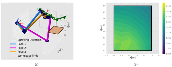
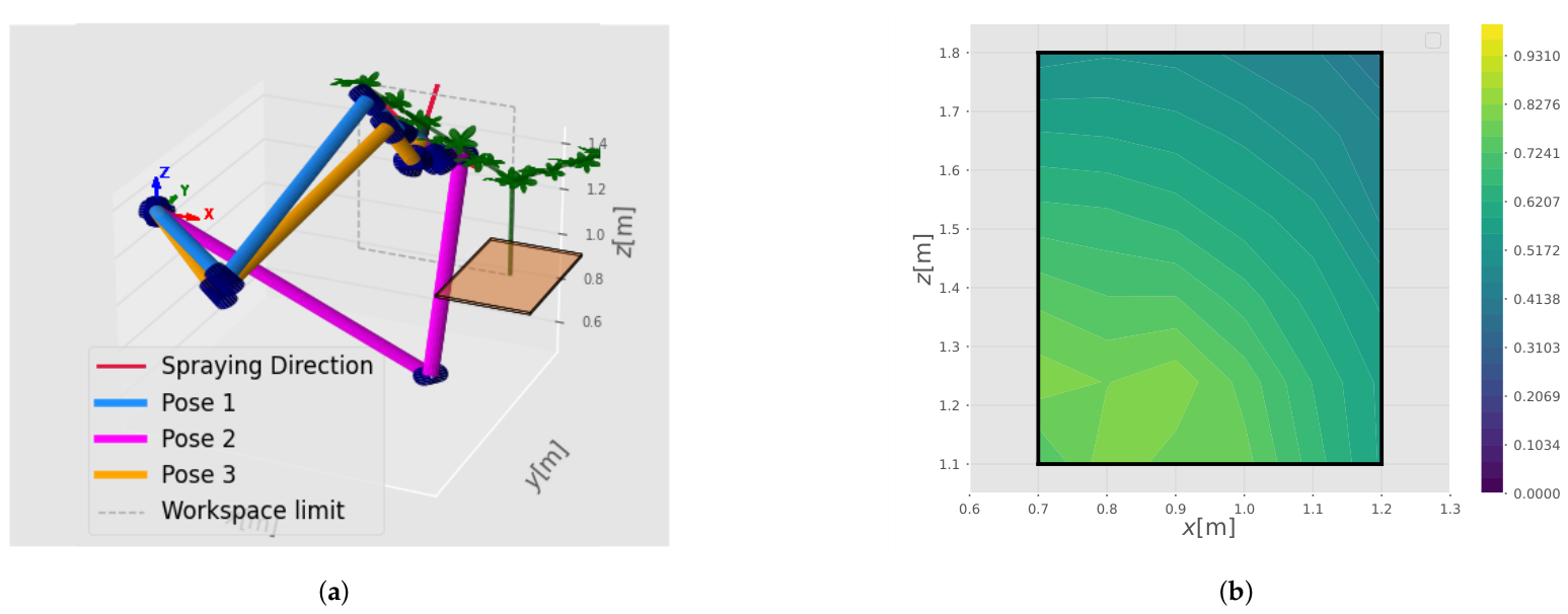
The capability to orient the end effector in several directions of the obtained design $F_1$ of Table 5 for the manipulator $RRR$ + wrist manipulator is evaluated by considering several poses obtained using Algorithm 1. The same Cartesian position ${\mathbf{t}}_{\mathbf{w}}={\left[\begin{array}{ccc}0.9& 0& 1.6\end{array}\right]}^T$ is considered for the three evaluated poses presented in Figure 9a. Pose 1 maximizes the manipulator’s reachability Index for the design $F_1$; it is worth noting that the pose that maximizes the local orientation capability was selected to evaluate the kinematic dexterity. Moreover, poses 2 and 3 present alternative manipulator positioning options for orienting the spraying nozzle during the spraying task (see Figure 9a). Additionally, the local dexterity over the workspace is considered for the poses that maximize reachability. The Local Conditioning Index reveals a distinct diagonal performance gradient across the flat rectangular workspace, with high kinematic dexterity in the bottom-left region peaking at 0.815 and a systematic degradation toward the upper-right corner, where it drops to a minimum of 0.412. For practical path planning, this specific design ensures high-precision tasks, as the minimum Local Conditioning Index remains high, preventing joint binding and control instability.

Figure 9. Performance analysis of $F_1$ solution of $RRR$ + wrist manipulator presented in Table 4: (a) Assessment of several poses for the same Cartesian position of the end effector. (b) Local Conditioning Index ($1/\kappa \left({\mathbf{J}}_{\mathbf{t}}(\mathbf{x},\mathbf{q})\right)$) over the desired workspace $\mathbf{w}$.

3.5. Manipulator Evaluation in a Virtual Vineyard Environment

The PyBullet simulator was used in Python to implement a motion-planning framework to evaluate the performance of the $RRR$ + wrist manipulator design for the spraying task. PyBullet is an intuitive Python framework for simulating physics, robotic architectures, and machine learning environments [29].

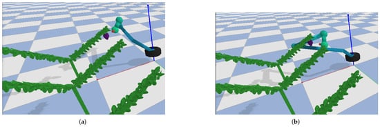
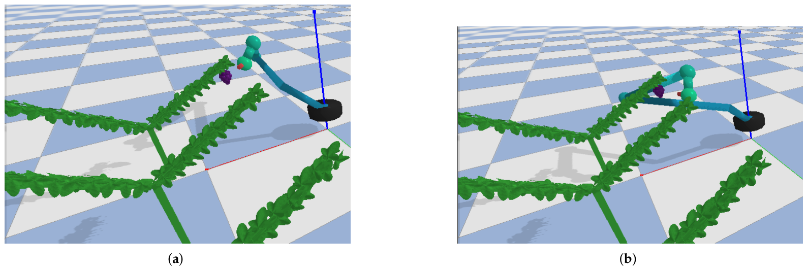
The PyBullet environment enables inverse and forward kinematics, motion planning, control, and visualization. A continuous orbital spraying trajectory around the target grape cluster that consists of a continuous quintic polynomial interpolation applied over a sweep angle range of $[-{60}^{\circ },+{60}^{\circ }]$ at $r_{\mathrm{orbit}}=0.28\mathrm{m}$ with the start position (Figure 10a) and end position (Figure 10b), was simulated with full multibody dynamics to quantify the dynamic feasibility of the optimal kinematic structure.

Figure 10. Illustration of $RRR$ + wrist manipulator performing a continuous orbital spraying trajectory around the target grape cluster using PyBullet: (a) start position (b) end position.

The manipulator achieved a peak joint torque demand of only $36.44\mathrm{Nm}$, well within the nominal effort capacity of industrial actuators. The nozzle maintained a mean Cartesian target-reaching offset of $45.06\mathrm{mm}$ around the grape cluster, attributable to the wrist length Tool Center Point (TCP), which falls comfortably within the effective swath radius of vineyard spray nozzles. A $100\%\mathrm{collision}\text{-}\mathrm{free}\mathrm{completion}\mathrm{rate}$ was achieved across a “Y”-shaped vineyard, validating both the kinematic synthesis and the obstacle avoidance clearance in this canopy structure.

Finally, the design variables $\mathbf{x}$ derived from the DH parameters are used to obtain a Unified Robot Description Format (URDF) file [30]. Furthermore, the URDF serves as a template for rapid workspace prototyping and can be integrated into a ROS/Gazebo ecosystem. This extension is essential to bridge the gap between kinematic design synthesis and full rigid-body dynamic validation.

4. Conclusions

This manuscript presented a multi-objective design optimization framework applied to a 6-DOF robotic manipulator for precision agricultural tasks, specifically targeting vineyard spraying. The mechanical performance was evaluated using kinematic and dynamic models to maximize kinematic dexterity quantified by the global conditioning index ($GCI$) and to minimize actuator power consumption along an operational trajectory. In addition, the global posture index ($GPI$) and the required workspace evaluation were included in the optimization framework as inequality constraints to obtain practical designs.

The multi-objective framework applied to eight different manipulator architectures established a performance criterion between the serial 6-DOF robotic manipulator topologies. NSGA-II was selected as the multi-objective solver due to its superior overall robustness across all evaluated manipulator architectures. In addition, the Pareto trade-offs established the theoretical foundation for the subsequent kinematic trajectory validation stage, which was directly verified along realistic task paths to confirm their simulated dynamic feasibility. Therefore, a comparative evaluation revealed distinct functional trade-offs:

• The fully prismatic ($PPP$) architecture achieved peak kinematic dexterity ($GCI=1.0$) with moderate mechanical power demand; however, its fixed joint axes limit its ability to execute complex, multi-directional spraying maneuvers required for deep canopy penetration.
• Conversely, the fully revolute ($RRR$) architecture demonstrated high posture flexibility and superior directional dexterity (${\Delta }_{\theta }$), making it ideal for penetrating dense grape foliage despite higher dynamic joint torques.
• The hybrid $RPR$ and $RPP$ architectures provided balanced Pareto-optimal trade-offs, as distal prismatic joints reduce active moving inertia and dynamic torques while revolute joints preserve nozzle dexterity.
• In contrast, $PRR$ and $PRP$ configurations featuring base-prismatic joints exhibited poor overall performance due to constrained reachability and elevated actuator mechanical demand.

The results of this study established a suitable methodology for selecting manipulator topologies and corresponding geometric parameters for precision vineyard spraying, helping designers balance kinematic dexterity with actuator power requirements. Future experimental validation will enable the development of physical prototypes and field testing.

References

- Gonzalez-de Santos, P.; Ribeiro, A.; Fernandez-Quintanilla, C.; Lopez-Granados, F.; Brandstoetter, M.; Tomic, S.; Pedrazzi, S.; Peruzzi, A.; Pajares, G.; Kaplanis, G.; et al. Fleets of robots for environmentally-safe pest control in agriculture. Precis. Agric. 2017, 18, 574–614. [Google Scholar] [CrossRef] [Scilit]
- Molaei, F.; Ghatrehsamani, S. Kinematic-based multi-objective design optimization of a grapevine pruning robotic manipulator. AgriEngineering 2022, 4, 606–625. [Google Scholar] [CrossRef] [Scilit]
- Stavridis, S.; Droukas, L.; Doulgeri, Z. Bimanual grape manipulation for human-inspired robotic harvesting. IEEE/ASME Trans. Mechatron. 2024, 30, 2722–2732. [Google Scholar] [CrossRef] [Scilit]
- Lytridis, C.; Bazinas, C.; Kalathas, I.; Siavalas, G.; Tsakmakis, C.; Spirantis, T.; Badeka, E.; Pachidis, T.; Kaburlasos, V.G. Cooperative grape harvesting using heterogeneous autonomous robots. Robotics 2023, 12, 147. [Google Scholar] [CrossRef] [Scilit]
- Xu, Z.; Liu, J.; Wang, J.; Cai, L.; Jin, Y.; Zhao, S.; Xie, B. Realtime picking point decision algorithm of trellis grape for high-speed robotic cut-and-catch harvesting. Agronomy 2023, 13, 1618. [Google Scholar] [CrossRef] [Scilit]
- Williams, H.; Smith, D.; Shahabi, J.; Gee, T.; Nejati, M.; McGuinness, B.; Black, K.; Tobias, J.; Jangali, R.; Lim, H.; et al. Modelling wine grapevines for autonomous robotic cane pruning. Biosyst. Eng. 2023, 235, 31–49. [Google Scholar] [CrossRef] [Scilit]
- Fernandes, M.; Gamba, J.D.; Pelusi, F.; Bratta, A.; Caldwell, D.; Poni, S.; Gatti, M.; Semini, C. Grapevine winter pruning: Merging 2D segmentation and 3D point clouds for pruning point generation. Comput. Electron. Agric. 2025, 237, 110589. [Google Scholar] [CrossRef] [Scilit]
- Azriel, R.; Degani, O.; Bechar, A. A Methodology to Characterize an Optimal Robotic Manipulator Using PSO and ML Algorithms for Selective and Site-Specific Spraying Tasks in Vineyards. Robotics 2025, 14, 58. [Google Scholar] [CrossRef] [Scilit]
- Khiali, E.; Marchetti, A.; Ribolla, G.; Negrello, F.; Corsanici, M.; Tincani, V.; Bicchi, A.; Previdi, F.; Catalano, M.G. Towards a Robotic Platform for Precision Vineyard Operations. IEEE Access 2026, 14, 23495–23512. [Google Scholar]
- Liu, E.; Gold, K.M.; Cadle-Davidson, L.; Kanaley, K.; Combs, D.; Jiang, Y. PhytoPatholoBot: Autonomous Ground Robot for Near-Real-Time Disease Scouting in the Vineyard. J. Field Robot. 2026, 43, 442–453. [Google Scholar] [CrossRef] [Scilit]
- Yang, Z.; Khan, Z.; Shen, Y.; Liu, H. An Efficient Embedded Vision Framework for Real-Time Grapes Vineyard Unhealthy Leaves Detection and Precision Guided Spraying. IEEE Trans. Autom. Sci. Eng. 2026, 23, 10718–10729. [Google Scholar] [CrossRef] [Scilit]
- Patel, S.; Sobh, T. Task based synthesis of serial manipulators. J. Adv. Res. 2015, 6, 479–492. [Google Scholar] [CrossRef] [Scilit]
- Lara-Molina, F.A.; Dumur, D.; Assolari Takano, K. Multi-objective optimal design of flexible-joint parallel robot. Eng. Comput. 2018, 35, 2775–2801. [Google Scholar] [CrossRef] [Scilit]
- Bloch, V.; Degani, A.; Bechar, A. A methodology of orchard architecture design for an optimal harvesting robot. Biosyst. Eng. 2018, 166, 126–137. [Google Scholar] [CrossRef] [Scilit]
- Huczala, D.; Kot, T.; Pfurner, M.; Heczko, D.; Oščádal, P.; Mostỳn, V. Initial estimation of kinematic structure of a robotic manipulator as an input for its synthesis. Appl. Sci. 2021, 11, 3548. [Google Scholar] [CrossRef] [Scilit]
- Ma, Y.; Feng, Q.; Sun, Y.; Guo, X.; Zhang, W.; Wang, B.; Chen, L. Optimized Design of Robotic Arm for Tomato Branch Pruning in Greenhouses. Agriculture 2024, 14, 359. [Google Scholar] [CrossRef] [Scilit]
- Soleimani, A. The soft computing approaches in optimising multi-objective mechanical design of a weeding robot. Smart Agric. Technol. 2024, 9, 100674. [Google Scholar] [CrossRef] [Scilit]
- Peng, C.; Feng, Q.; Guo, Z.; Ma, Y.; Li, Y.; Zhang, Y.; Gao, L. Structural Parameter Optimization of a Tomato Robotic Harvesting Arm: Considering Collision-Free Operation Requirements. Plants 2024, 13, 3211. [Google Scholar] [CrossRef] [Scilit]
- Cao, X.; Yan, H.; Huang, Z.; Ai, S.; Xu, Y.; Fu, R.; Zou, X. A multi-objective particle swarm optimization for trajectory planning of fruit picking manipulator. Agronomy 2021, 11, 2286. [Google Scholar] [CrossRef] [Scilit]
- Rybak, L.; Carbone, G.; Mohan, S.; Gaponenko, E.; Malyshev, D.; Voloshkin, A. New design and construction of a mechanical gripping device with a telescopic link of a fruit harvesting robot. Robotica 2025, 43, 69–85. [Google Scholar] [CrossRef] [Scilit]
- Chitre, N.; Dogra, A.; Singla, E. Optimal synthesis of reconfigurable manipulators for robotic assistance in vertical farming. Robotica 2023, 41, 2283–2297. [Google Scholar] [CrossRef] [Scilit]
- Yoshikawa, T. Dynamic manipulability of robot manipulators. Trans. Soc. Instrum. Control Eng. 1985, 21, 970–975. [Google Scholar] [CrossRef] [Scilit]
- Siciliano, B.; Sciavicco, L.; Villani, L.; Oriolo, G. Robotics: Modelling, Planning and Control; Springer: Berlin/Heidelberg, Germany, 2009. [Google Scholar]
- Angeles, J. Fundamentals of Robotic Mechanical Systems: Theory, Methods, and Algorithms; Springer: Berlin/Heidelberg, Germany, 2003. [Google Scholar]
- Corke, P.; Haviland, J. Not your grandmother’s toolbox–the Robotics Toolbox reinvented for Python. In Proceedings of the 2021 IEEE International Conference on Robotics and Automation (ICRA); IEEE: New York, NY, USA, 2021; pp. 11357–11363. [Google Scholar]
- Gosselin, C.; Angeles, J. A Global Performance Index for the Kinematic Optimization of Robotic Manipulators. J. Mech. Des. 1991, 113, 220–226. [Google Scholar] [CrossRef] [Scilit]
- Blank, J.; Deb, K. Pymoo: Multi-objective optimization in python. IEEE Access 2020, 8, 89497–89509. [Google Scholar] [CrossRef] [Scilit]
- Deb, K.; Pratap, A.; Agarwal, S.; Meyarivan, T. A fast and elitist multiobjective genetic algorithm: NSGA-II. IEEE Trans. Evol. Comput. 2002, 6, 182–197. [Google Scholar] [CrossRef] [Scilit]
- Panerati, J.; Zheng, H.; Zhou, S.; Xu, J.; Prorok, A.; Schoellig, A.P. Learning to fly—A gym environment with pybullet physics for reinforcement learning of multi-agent quadcopter control. In Proceedings of the 2021 IEEE/RSJ International Conference on Intelligent Robots and Systems (IROS); IEEE: New York, NY, USA, 2021; pp. 7512–7519. [Google Scholar]
- Tola, D.; Corke, P. Understanding urdf: A survey based on user experience. In Proceedings of the 2023 IEEE 19th International Conference on Automation Science and Engineering (CASE); IEEE: New York, NY, USA, 2023; pp. 1–7. [Google Scholar]
- Denavit, J.; Hartenberg, R.S. A Kinematic Notation for Lower-Pair Mechanisms Based on Matrices. J. Appl. Mech. 2021, 22, 215–221. [Google Scholar]
Disclaimer/Publisher’s Note: The statements, opinions and data contained in all publications are solely those of the individual author(s) and contributor(s) and not of MDPI and/or the editor(s). MDPI and/or the editor(s) disclaim responsibility for any injury to people or property resulting from any ideas, methods, instructions or products referred to in the content. |
© 2026 by the authors. Licensee MDPI, Basel, Switzerland. This article is an open access article distributed under the terms and conditions of the Creative Commons Attribution (CC BY) license.