


Abstract
We pose and study the inverse problem of the chiral low-energy constants (LECs): with our re-implemented and checked Yang large- forward operator (reproducing all eight LECs of Yang’s Table I within , four within ), we use the experimental LECs of Pan et al. and the lattice quark mass function of Oliveira et al. as data to invert for the quark self-energy . (1) Treating as a free function results in a multimodal posterior; two independent analyses locate the LEC information window at ∼0.5– and distinguish the profile-sensitive – from the comparatively profile-rigid under the tested changes in . (2) Parametrizing through the kernel of the gap equation (Maris–Tandy/Qin–Chang) collapses the inversion to three kernel parameters : the resulting posterior is unimodal, the lattice data and LECs are fitted simultaneously, and the uncertainties in at representative momenta are reduced by factors of 2–4. (3) The fitted result contains four apparent deviations from Pan/FLAG. A proper-time regulator scan examines their response to the forward prescription. The apparent tensions in , and the condensate are not particularly stable under the checks performed, whereas remains above the Pan central value throughout the scan. It also varies little across the two kernel realizations and the exploratory profile proxy. At the representative point, differs by from the quoted Pan value ; the condensate-based comparison and the scalar resonance-saturation estimate show the same tendency. These results support a possible tension associated with the scalar-channel LEC within the tested leading- rainbow construction.
1. Introduction
The low-energy constants (LECs) of chiral perturbation theory (ChPT) encode the dynamics of QCD in the pseudoscalar-meson sector [1,2,3,4,5]. A long-standing line of research connects them to the underlying theory through the quark self-energy : Yang, Wang, Kuang and Lu [6] worked in the large- limit [7,8] within an improved ladder approximation, expressing the LECs as a set of momentum integrals over and its derivatives (), and obtained values broadly consistent with experiment by solving the Schwinger–Dyson equation [9,10,11]. The forward map is thereby well defined; yet its inverse problem—what the measured set of LECs implies for the self-energy, and what that comparison in turn reveals about the framework itself—has not been studied.
This paper poses and studies that inverse problem directly. Using the experimentally determined LECs of Pan et al. [12] together with the lattice quark mass function of Oliveira et al. [13] as data, we ask which self-energies are compatible with them under the Yang forward operator. We re-implement the operator in full (15 integrals, six auxiliary polynomials, the explicit constant- subtraction, and the LEC assembly) as a differentiable PyTorch [14] map, and check it against Yang’s Table I (all eight LECs within , four within ; Section 2), including an audit of the remaining numerical discrepancies.
Two features make the inverse problem at once nontrivial and ultimately informative:
(i) It is underdetermined and multimodal. Six data points (or thirteen when the lattice pins are included) constrain a -point discretization of . Treating as a free function, the posterior is severely underdetermined. We show (Section 3) that the LEC data carry information about only in a mid-momentum window – (located by two independent analyses); moreover, different LECs respond differently to the tested changes in —the profile-sensitive – versus the comparatively profile-rigid (Section 5)—a classification that guides the subsequent diagnostics.
(ii) It can be constrained by physical priors. Rather than fitting a free , we parametrize it through the kernel of the gap equation: replacing Yang’s bare interaction with the Maris–Tandy/Qin–Chang effective interaction [15,16], we solve the (rainbow, ) gap equation, generating a self-energy with the expected ultraviolet tail, monotonicity and dynamical chiral symmetry breaking built in. The inverse problem then collapses to three kernel parameters ; the resulting posterior is unimodal (Section 4).
These features enable a diagnostic comparison of four apparent deviations from Pan/FLAG. We use a proper-time regulator scan to examine their response to variations in the forward prescription. Within the checks performed, the apparent tensions in , and the condensate are not particularly stable, while the independent -resonance estimate for is close to Pan [17,18]. shows a different pattern: it remains above the Pan central value throughout the regulator scan, responds only weakly to the tested changes in the profile, and varies little across the two kernel realizations and the exploratory profile proxy. The condensate-based comparison and the scalar resonance-saturation estimate point in the same direction, supporting a possible tension within the tested leading- rainbow construction (Section 5).
The paper is organized as follows. Section 2 presents the forward operator and its implementation check; Section 3 establishes the multimodality diagnosis of the free- inversion and the LEC information window; Section 4 carries out the kernel-parametrized inversion; Section 5 examines the four apparent deviations using the LEC profile split, proper-time regulator scan, and resonance-saturation comparisons, and the two tested kernel realizations; Section 6 summarizes the conclusions and discusses them.
2. The Forward Operator
Following Yang et al. [6,19], in the large- limit the low-energy constants are given by linear combinations of 15 integrals (their Equation (25)). Five of the vanish identically (), so the large- prediction is ; the gap to the nonzero experimental values is the known deviation, and we exclude from the likelihood, keeping them as a model-bias check.
The remaining 10 nonzero integrals (Yang Equation (36)) involve the self-energy and its first and second derivatives together with six auxiliary polynomials – (Yang Equation (38)). The Wick-rotated integration measure is
where is the Euclidean (dimensionless) and is the Schwinger regulator cutoff; the Wick rotation takes , , . After inserting the vanishing , the six LECs entering the likelihood are assembled from the (Yang Equation (25), ) as
where is determined self-consistently by (Yang Equation (34)). All operations are implemented as PyTorch tensors, ensuring automatic differentiability; a single forward pass takes ∼30 ms. The forward pass requires a dense grid for the explicit constant- subtraction, for which we take points. Throughout this paper, numerical values quoted for the without an explicit power of ten are given in units of .
As an implementation check, we digitize the Model A self-energy of Yang’s Figure 2 [6], interpolate it onto the grid as forward input, and compare it against the first row of Yang’s Table I (Table 1): all eight LECs agree within , four of them within , and the self-consistency residual is .
Table 1.
Implementation check of the forward operator on the Yang Model A baseline. is the exact large- prediction, independent of the fit; is checked self-consistently through the independent Pagels–Stokar relation [20].
To examine the likely origin of the -level implementation-check residuals, we varied the quadrature density and domain, floating-point precision, ultraviolet continuation of the digitized self-energy, an independent digitization of the published curve, and the finite numerical realization of the constant- subtraction. Grid and precision effects are below about ; across the converged integration domains, the reported LECs change by at most about (and by at most ). The ultraviolet continuation and re-digitization produce observable-dependent shifts of several percent—about 4– for and 6– for . The finite subtraction realization is more consequential: the tested variations are at the tens-of-percent level for , below about for , about for , and about 10– for . Because the numerical profile and complete implementation details were not published, the origins of these discrepancies cannot be determined uniquely. They do not alter the inverse-problem formulation or the differentiation, optimization and sampling procedures, but they do affect the quantitative interpretation of the fitted outputs; this point is taken up in Section 5.
3. Free- Inversion: Multimodality and the LEC Information Window
3.1. Single-Chain Fit
Bayesian setup. We discretize into points in the logarithmic momentum variable , with the posterior . The likelihood takes the Gaussian form
where the first term contains Pan’s six LECs (), with the corresponding block of Pan’s covariance [12]; the large--vanishing are excluded. is assembled via Equation (2), and the second term contains Oliveira’s 7 lattice pins [13], giving about 13 observations in total. The prior is a zero-mean Gaussian process [21] with RBF covariance (, , ). This prior is chosen because it encodes only the weakest physical constraint—smoothness of the self-energy: in the strongly underdetermined inversion of a -dimensional curve from observations, it supplies the necessary physical prior without imposing excessive constraints.
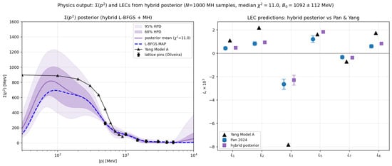
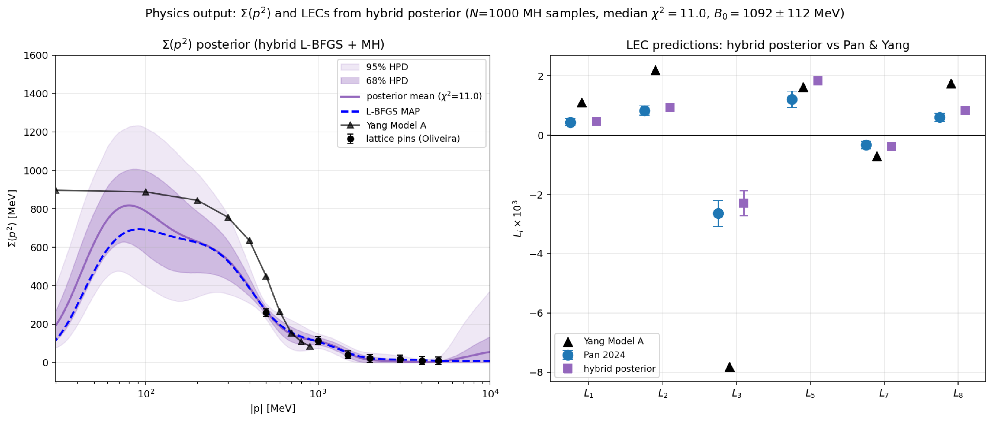
Single-chain result: We find the MAP with L-BFGS [22], then sample a single chain with Hessian-preconditioned Metropolis [23,24]. The single chain already achieves a good fit (): the posterior band passes through all 7 Oliveira lattice points and reproduces Pan’s LECs (Figure 1). As far as fitting the data themselves is concerned, the free- scheme can therefore reproduce the modern LEC data within the Yang framework.
Figure 1.
Posterior of the free- inversion (L-BFGS MAP + Hessian-MH). Left: HPD band of , posterior mean (), L-BFGS MAP, Yang Model A and Oliveira lattice points; right: LEC predictions (posterior vs. Pan et al. [12] and Yang). The band passes through all lattice points and reproduces the LECs; the single chain already reaches .
3.2. Multiple Chains Reveal Multimodality
A good single-chain fit does not imply that the posterior is unique. We repeat the sampling with 12 independent chains, each with steps, and compute the Gelman–Rubin [25] (Table 2). Quantities constrained by the data agree across chains (, ESS for ), but the directions not constrained by the data do not converge over the sampled runs (median componentwise , max , with not decreasing to even after total steps): different chains stabilize on different shapes, i.e., the posterior is multimodal. Correspondingly, the deep-IR region appears unconstrained ().
Table 2.
Posterior and convergence diagnostics of the free- inversion with multiple chains (12 chains, each with steps). Quantities constrained by data agree across chains; the of unconstrained directions stays high, indicating posterior multimodality.
In other words, although the free- inversion can fit the data, it does not yield a unique, well-constrained : 13 data points are insufficient to pin down a 1000-dimensional curve, and the excess degrees of freedom manifest as multimodality. At the same time, the contrast between the good fit in the mid-momentum region and the unconstrained deep IR suggests that the information on in the deep IR is insufficient. We therefore perform an LEC-sensitivity test in both the forward and the inverse directions to identify the cause of the multimodality of the free- posterior. The posterior and diagnostics in Table 2 show the multimodality across chains.
3.3. Forward/Inverse Scans Locate the Information Window
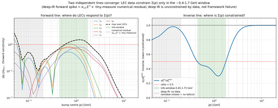
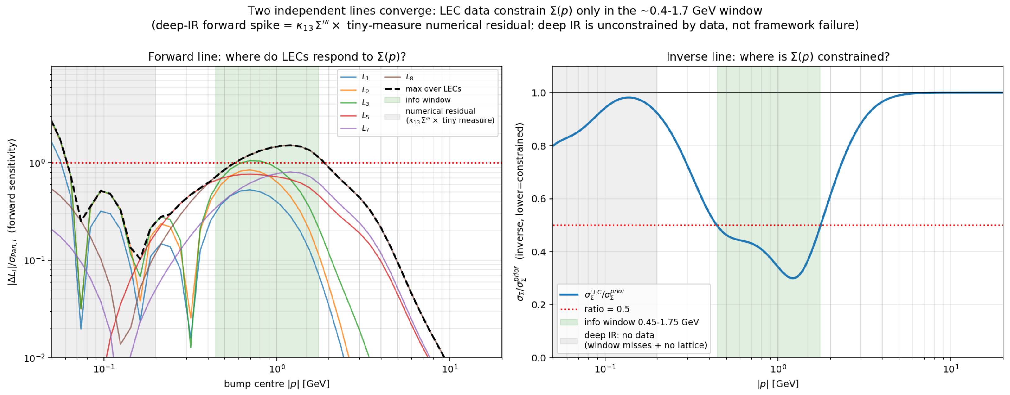
Forward line (sensitivity kernel). We perturb the baseline (L-BFGS MAP) with a Gaussian bump whose width matches the prior length scale, scan it across momentum, and record the response . The region in which the maximum response over the six LECs exceeds 1 is –. Inverse line (posterior width). Propagating the posterior width from the MAP via the LEC-only Gauss–Newton Hessian, the ratio of posterior to prior width drops below over –, with the strongest constraint at . The two windows coincide at ∼0.5–1.75 GeV (Figure 2). Outside the window, the data carry little information, so the deep IR is weakly constrained. This reflects the limited sensitivity of the LECs to in that region.
Figure 2.
Two independent lines close on the ∼0.5– information window. Left: forward sensitivity kernel, where the red dotted line marks the unit-sensitivity threshold; right: inverse posterior-to-prior width ratio, where the black horizontal line marks equality of the posterior and prior widths. The small forward peak in the deep IR is an unphysical numerical residual arising from the product of and a tiny measure.
3.4. Cross-Validation and Summary
As a cross-validation of the LECs’ predictive power for , we remove the two lattice pins at and and refit using only the 6 LECs plus the 5 outer pins. The held-out prediction agrees with the removed lattice value within , with a prediction width of only of the prior, indicating a constraint from the retained data rather than direct use of the removed pins.
Summary: Together, the two tests characterize the free- inversion. First, the information-window analysis from two independent approaches shows that the LECs are insensitive to outside the window (especially the deep IR); second, the cross-validation above shows that within the sensitive region the LECs and lattice data provide constraints supported by the held-out comparison ( agreement, with a width only of the prior). In the mid-momentum region where the data carry information, the free- inversion therefore gives a data-constrained . The multimodality exposed in Section 3.2 is associated with underdetermination in the deep IR: the there is only weakly constrained, and the excess degrees of freedom manifest as multimodality. This information deficit outside the window is the starting point for Section 4, where a physical kernel supplies the deep-IR degrees of freedom.
4. Kernel-Parametrized Inversion
4.1. From Fitting to Fitting the Kernel
The free- multimodality arises from using 13 data points to constrain degrees of freedom. Rather than fitting itself, we fit the kernel of the gap equation that produces , compressing the curve’s degrees of freedom to a few physical parameters. The large number of parameters allows the function to vary widely where deep-IR information is limited, whereas with only a few parameters, constraints from the LEC information window can propagate into the deep IR through the functional form. The kernel replacement also addresses a weakness of the Yang framework: Yang’s bare interaction is , whose running coupling lacks a first-principles definition in the infrared and therefore requires an explicit modeling and regularization prescription. We replace it with the Maris–Tandy/Qin–Chang effective interaction [15,16] ,
which characterizes the infrared strength by an infrared-finite Gaussian enhancement (strength D, width ) and incorporates the expected ultraviolet asymptotic behavior through the logarithmic term. Its canonical parametrization is calibrated against hadron phenomenology and has an explicit infrared form. This replaces the infrared prescription of Yang’s bare by an explicitly parametrized interaction for the subsequent inversion. We retain the truncation to keep the Yang forward operator (built on ) usable as is—the forward operator, the data layer and the assembly are all reused, and only the source of is replaced. The self-energy is constrained by the gap equation, and the dimensionality collapses from 1000 to 3.
4.2. Gap Equation and Ultraviolet-Anchor Validation
The Euclidean, Landau-gauge, rainbow, scalar equation [26] is
with . The two-dimensional angular integral must be evaluated explicitly (Yang’s angular approximation is exact only for the bare kernel and fails when the kernel is replaced); for the bare kernel our numerical agrees with the analytic expression to . The overall constant is calibrated by physical anchors: a UV anchor (, validated analytically) plus the asymptotic tail (the chiral-solution UV logarithmic slope measured as over , consistent with Yang Equation (46)). Before using the solver in the inverse analysis, we also check it at the canonical MT parameter point : the coupled equation gives , , and , at the expected constituent-mass scale quoted in the MT/FLAG literature [15,27,28]. This comparison is used as a reasonable implementation check for the coupled gap solver.
4.3. Three-Parameter Fit Results
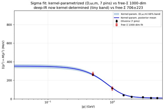
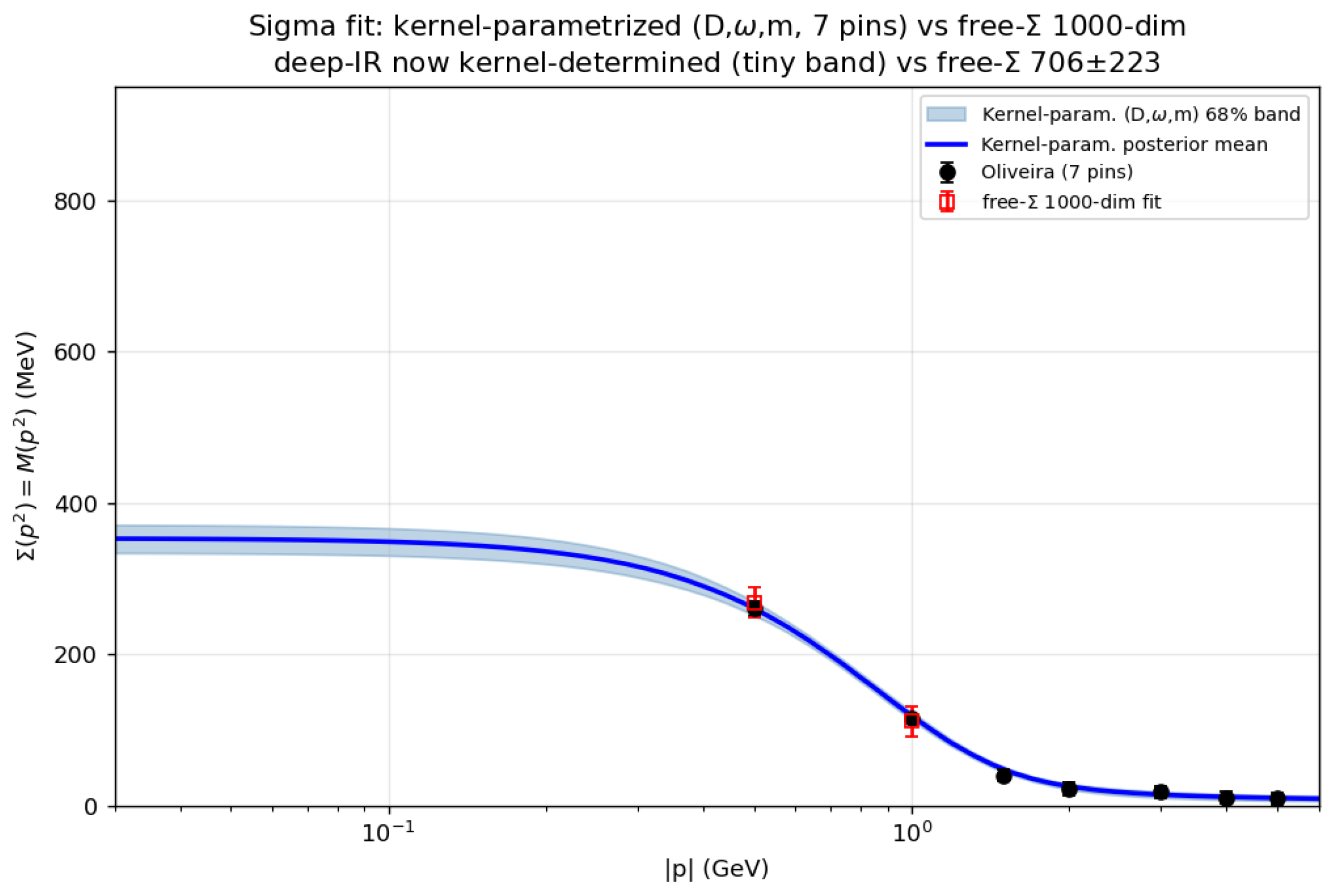
The posterior , where combines contributions from the Pan LEC data, the Oliveira lattice data, and the anchor, is computed directly on a three-dimensional grid in , without MCMC sampling (∼0.6 s per point). The joint fit gives , , ; all 7 lattice points are fitted simultaneously (), yielding , , with posterior uncertainties 2–4 times smaller than those from the 1000-dimensional free inversion reported in Table 2 (Figure 3). Because there are only three parameters and the posterior is integrated directly on the grid, the evaluated posterior is unimodal on the tested grid: the multimodality and non-converging of the 1000-dimensional free inversion in Section 3.2 are not observed here. This supports the interpretation that the excess deep-IR degrees of freedom drive the multimodality of the free inversion; compressing to three kernel parameters removes those degrees of freedom in the present fit. The resulting LECs are listed in Table 3, with small uncertainties (), providing a baseline for the framework diagnosis of Section 5.
Figure 3.
Posterior band (blue) of the kernel-parametrized inversion , passing through all 7 Oliveira lattice points (black).
Table 3.
LECs from the three-parameter kernel-parametrized fit (; central value from the best self-energy, uncertainties from the three-parameter posterior standard deviations; units , pull relative to Pan [12]). The posterior is unimodal and the uncertainties are small; the higher values relative to Pan are analyzed in Section 5.
The fitted D differs from the canonical value quoted above, mainly because the latter comes from a calibration with coupled dynamics and meson Bethe–Salpeter calculations [15,16], whereas the present inverse fit fixes to reuse the Yang forward operator and refits D within this reduced equation. At the fitted point, the Pagels–Stokar estimate [20] of the pion decay constant is , in close agreement with the input value . This agreement provides a basic pion-sector consistency check and supports the physical plausibility of the present fit within the setup.
5. A Possible Tension in the Leading- Rainbow Framework
A comparison of the framework forward predictions (kernel-parametrized LECs, Table 3) with Pan/FLAG [12,28] reveals four apparent deviations: , , the chiral condensate and . This section compares their responses to identifiable regulator and -shape variations. Within the variations examined here, the apparent deviations in , and the condensate are less persistent, whereas the discrepancy is more persistent. The comparison rests on the response split of the LECs to the profile (Section 5.1) and the proper-time regulator response (Section 5.2), followed by further diagnostics of (Section 5.3 and Section 5.4).
5.1. Different Responses of the LECs to the Profile
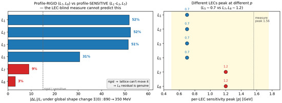
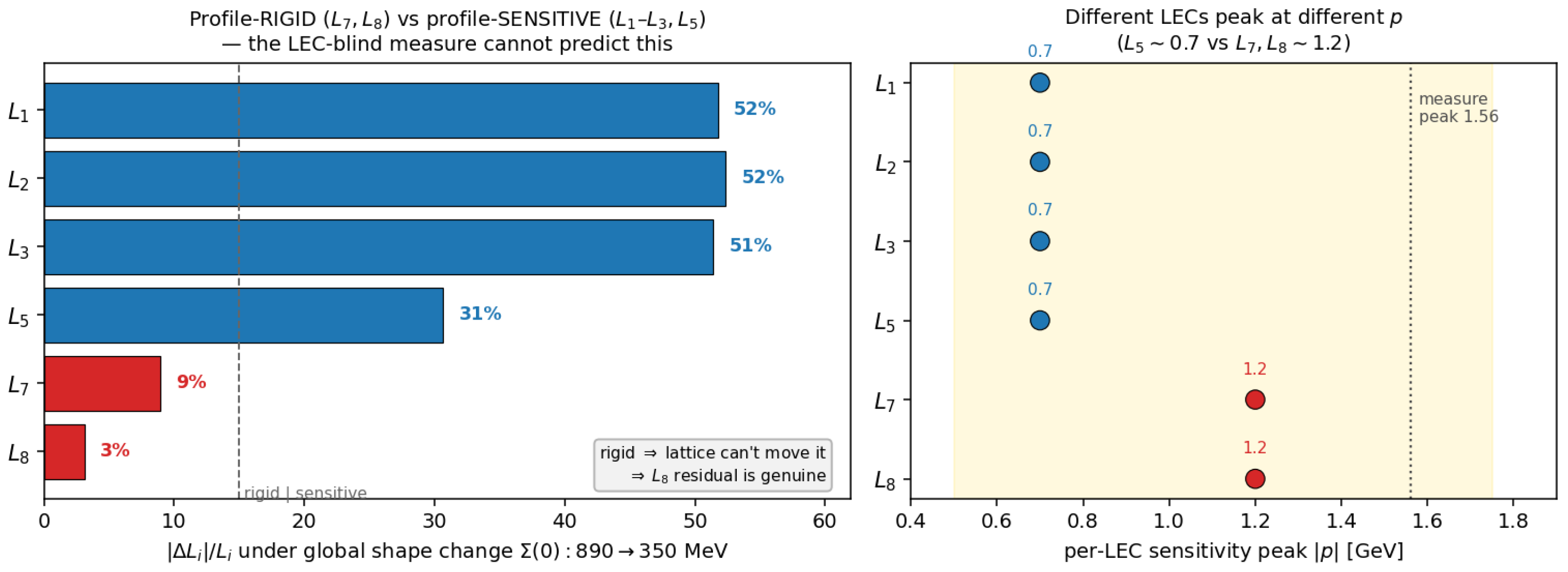
The LECs’ sensitivity to is concentrated in the mid-momentum information window (Section 3), but different LECs are affected differently by . When the kernel replacement changes the overall profile substantially (), – move by ∼50% and by (profile-sensitive), whereas move by only and (profile-rigid, Figure 4); the sensitivity-peak positions also differ (– at , at ). This split originates in the assembly structure.
Figure 4.
Comparatively profile-rigid () versus profile-sensitive (–) responses under the tested global profile change. Left: fractional shift of each LEC; right: position of each LEC’s sensitivity peak.
This comparison shows that the profile-sensitive – are strongly affected by the choice of /kernel, so replacing the kernel (Section 4) can move them away from the Yang bare-kernel prediction toward the modern values; are comparatively insensitive to this particular profile change at fixed forward prescription.
The fixed-prescription qualifier is important. The implementation audit in Section 2 finds a subtraction response below about for , about for , and about 10– for . Although not negligible, the subtraction responses of and are moderate compared with the tens-of-percent responses of and . In the present inverse fit and kernel-replacement comparison, the change in the shape of is the primary variation of interest. Combining this consideration with the moderate subtraction responses of and , we give priority in the subsequent analysis to these two comparatively profile-rigid LECs.
5.2. Proper-Time Regulator Sensitivity of , and
The three LECs carrying (Yang Equation (25)) are
The relation [3] enters together with the integrals, and both are recomputed self-consistently for the same self-energy at each proper-time regulator value . The ChPT renormalization scale enters directly in the definition and phenomenological comparison of the renormalized LECs , but incorporating this scale dependence consistently into the inverse fit is nontrivial. For example, the one-loop ChPT property [3,18] provides an additional constraint on the interpretation of the response. As a practical preliminary diagnostic, we therefore examine the response of the apparent deviations in , , and to a scan of the forward-model regulator . The aim is to identify which deviations remain comparatively persistent under this controlled variation and therefore merit priority in the subsequent analysis.
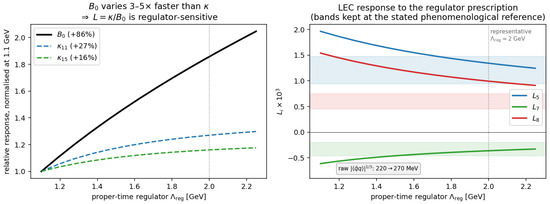
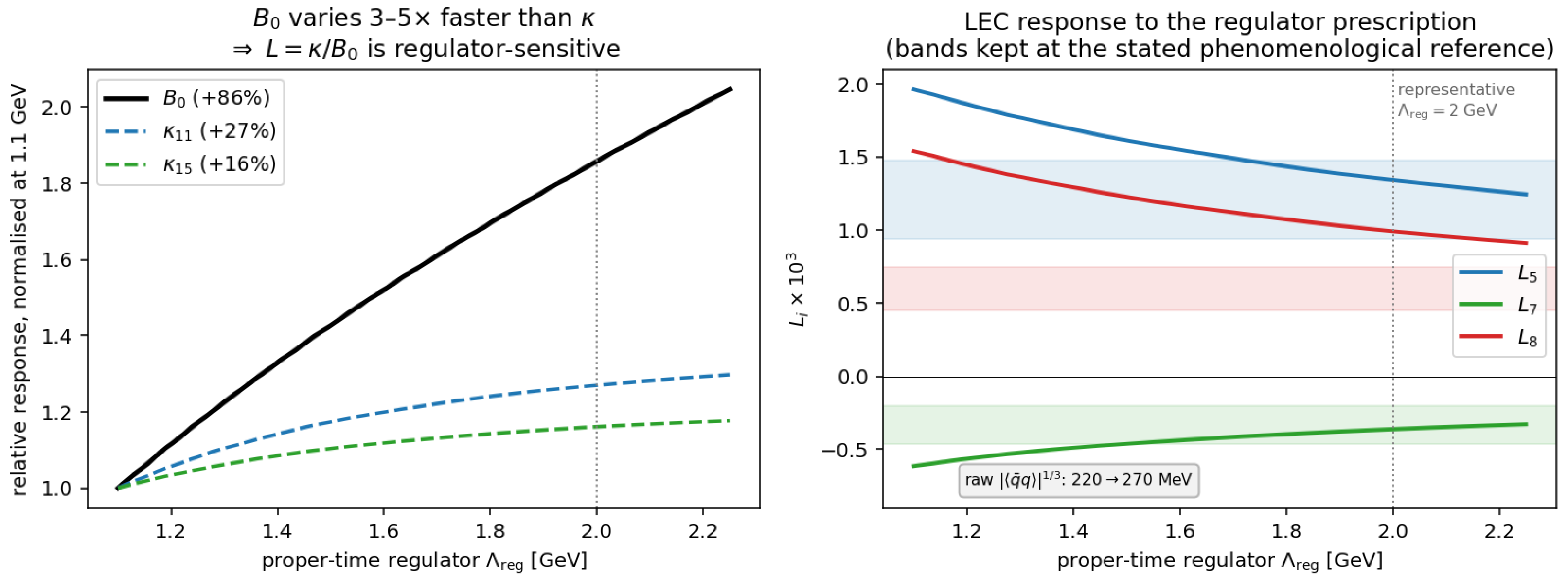
We perform a multipoint calculation in which the same self-energy is evaluated at 14 regulator values from to , with all and recomputed at every point (Figure 5). Table 4 lists two representative points. Between and , rises by , while the numerators rise by only 16–; consequently, , , and .
Figure 5.
The 14-point proper-time regulator scan. Left: relative responses of , and . Right: as functions of the proper-time regulator; the phenomenological bands are held fixed at their stated reference.
Table 4.
Representative points from the multipoint proper-time regulator scan (kernel-parametrized best self-energy).
Over the scanned interval, , and the condensate estimate all move toward the quoted Pan/FLAG values. For , an additional comparison independent of the present inversion is provided by the resonance-saturation -channel value [17,18] , which is close to both the framework value and the Pan value [12]. The condensate estimate changes from about 220 to , approaching the quoted FLAG value [28]. Across these diagnostic checks, the apparent tensions in , , and the condensate are not particularly stable; the following subsection therefore focuses on the more persistent candidate.
behaves differently in this diagnostic. Inverting the assembly relation with the baseline held fixed gives the effective required to reproduce each Pan central value: requires and requires , whereas requires , substantially higher than the values required for the former two. We therefore examine further in the following subsection.
5.3. Further Diagnostics of
At the representative point, . Comparison with the quoted Pan value [12] gives a numerical difference of . Across the 14-point scan over –, exhibits a different pattern from , , and the condensate: the latter three reach their quoted Pan/FLAG ranges, whereas remains above the Pan central value throughout. This contrast draws attention to the discrepancy.
The condensate provides a reference independent of the regulator scan. Using the Yang normalization [6] and the quoted FLAG value [28], the relation gives . The algebraic values obtained above with the baseline held fixed, for and for , lie near this condensate-based reference, whereas requires the substantially larger value .
A further external comparison is provided by resonance saturation. In the standard resonance-saturation decomposition [17,18], is saturated purely by the scalar channel (vector, axial-vector and contributions are all zero), with the large- scalar value . This agrees with the older phenomenological value , but is above the modern NLO value . By contrast, is saturated by the channel, whose estimate near is consistent with Pan. The regulator response, the condensate-based comparison and the resonance-saturation pattern all direct attention to within the leading large- framework. Omitted subleading scalar contributions provide a possible origin of this pattern [29].
5.4. Effects of Rainbow Truncation and Kernel Choice
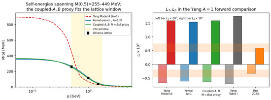
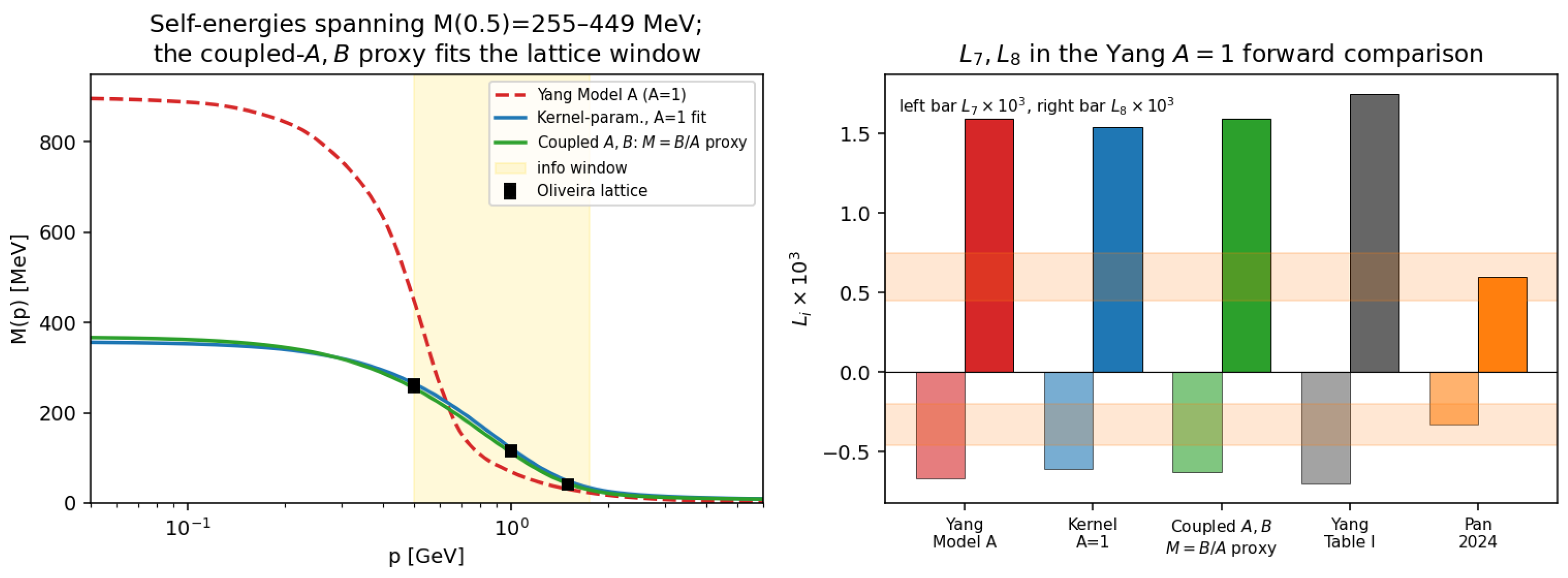
To examine the sensitivity of to the mass-function profile, we solve the coupled rainbow gap equations for and [15,16] and insert the resulting mass function into the existing Yang forward operator (; Table 5, Figure 6). Three input self-energies of very different profiles, with ranging from 255 to , give – in this common assembly, dominated by the scalar term (128–). Across the tested coupled parameter grid, the lattice-compatible proxies with give –. Thus, the mass-function substitution does not remove the discrepancy within the tested grid.
Table 5.
Results after the kernel replacement: varies only over a narrow range.
Figure 6.
Left: the three scalar input profiles coincide in the window and differ in the deep infrared. Right: the predictions for are ∼2–3 times the corresponding Pan et al. [12] values in the configurations shown. The orange horizontal bands denote the corresponding quoted Pan uncertainty intervals.
The result remains a profile proxy rather than a complete calculation of the LECs. The quoted range therefore characterizes the profile sensitivity within the unchanged assembly, rather than the uncertainty of a complete forward operator. Yang’s own Table I [6] gives , which itself lies above the modern Pan value, independently of the kernel replacement and inverse fit introduced in this work. Yang’s result, the MT/QC-based result and the exploratory proxy all yield high values across the tested profiles and the two kernel realizations, further strengthening the indication of a possible tension.
5.5. Summary
Of the four apparent deviations in the fitted result, those in , and the condensate are not persistent under the relevant diagnostic variations. and move substantially under the proper-time regulator scan, while the condensate comparison remains prescription-dependent. For , the independent -resonance estimate is also close to the Pan value. These results therefore leave only weak indications of tension in these three quantities.
displays a different pattern. It remains above the Pan central value throughout the proper-time regulator scan and remains high across the tested self-energy profiles, the two kernel realizations and the exploratory proxy. The effective required to reproduce the Pan central value, , is also substantially higher than the condensate-based reference and the values required for and . Moreover, the scalar resonance-saturation value itself lies above the modern Pan value. Taken together, these observations strengthen the indication of a possible tension localized in the scalar-channel LEC within the tested leading- rainbow construction.
6. Conclusions
We have turned the LEC-to-self-energy inverse problem into an end-to-end quantitative diagnosis. The main conclusions are as follows.
Method and diagnosis. We re-implemented the Yang large- forward operator and checked it against Yang’s Table I, reproducing all eight LECs within and four within , with self-consistency at the level. The implementation audit finds negligible grid and precision effects, percent-level responses to the digitized profile and its ultraviolet continuation, and larger observable-dependent responses to the subtraction prescription. Since the original numerical profile and full implementation details are not available, the origins of the remaining discrepancies cannot be determined uniquely, and these sensitivities are included in the interpretation of the LEC comparisons. Treating as a free function gives a multimodal posterior; two independent analyses locate the LEC information window at ∼0.5–, while the held-out prediction agrees with the removed lattice point within and has a width equal to of the prior. Parametrizing the gap equation by three kernel parameters yields a unimodal posterior on the tested grid, fits the lattice and LEC data simultaneously, and reduces the uncertainty in by a factor of 2–4.
Phenomenological indication: a possible Ptension in the tested leading- rainbow framework. The fitted result contains four apparent deviations from Pan/FLAG. We use the proper-time regulator scan to examine how these four apparent tensions respond to variations in the forward prescription. Within the checks performed, the apparent tensions in , and the condensate are not particularly stable, and the independent -resonance estimate for is close to the Pan value. shows a different pattern. Although it changes under the regulator and subtraction prescriptions, it remains above the Pan central value throughout the regulator scan. It also varies little across the two kernel realizations and the exploratory profile proxy. At the representative point, differs by from the quoted Pan value . The effective required to reproduce the Pan central value is , above the condensate-based reference , while the scalar resonance-saturation estimate is also above Pan. These observations support a possible tension associated with the scalar-channel LEC within the construction tested here.
Limitations and outlook. The present kernel comparison covers two interaction realizations, and the substitution is a profile-level diagnostic rather than a complete calculation of the LECs. A broader kernel comparison and a full forward operator would therefore be needed to assess general kernel and truncation dependence. Cross-validation of the kernel-parametrized inversion and a treatment beyond rainbow with a consistent Bethe–Salpeter equation [30,31,32] may be addressed in future work. More broadly, the method applies to inverse problems of similar structure (high-dimensional parameters, few observations, and a physically regularizable forward operator).
Author Contributions
Conceptualization, X.X. and D.-K.K.; methodology, X.X. and D.-K.K.; software, X.X.; validation, X.X.; formal analysis, X.X.; investigation, X.X.; data curation, X.X.; visualization, X.X.; writing—original draft preparation, X.X.; writing—review and editing, X.X. and D.-K.K.; resources, D.-K.K.; supervision, D.-K.K. All authors have read and agreed to the published version of the manuscript.
Funding
This research received no external funding.
Data Availability Statement
The original contributions presented in this study are included in the article. Further inquiries can be directed to the corresponding author.
Conflicts of Interest
The authors declare no conflicts of interest.
Abbreviations
The following abbreviations are used in this manuscript:
| ChPT | Chiral perturbation theory |
| LEC | Low-energy constant |
| QCD | Quantum chromodynamics |
| DSE | Dyson–Schwinger equation |
| MT | Maris–Tandy |
| QC | Qin–Chang |
| IR | Infrared |
| UV | Ultraviolet |
| MAP | Maximum a posteriori |
| HPD | Highest posterior density |
| ESS | Effective sample size |
| GP | Gaussian process |
| RBF | Radial basis function |
References
- Weinberg, S. Phenomenological Lagrangians. Physica A 1979, 96, 327–340. [Google Scholar] [CrossRef] [Scilit]
- Gasser, J.; Leutwyler, H. Chiral Perturbation Theory to One Loop. Ann. Phys. 1984, 158, 142–210. [Google Scholar] [CrossRef] [Scilit]
- Gasser, J.; Leutwyler, H. Chiral Perturbation Theory: Expansions in the Mass of the Strange Quark. Nucl. Phys. B 1985, 250, 465–516. [Google Scholar] [CrossRef] [Scilit]
- Scherer, S. Introduction to Chiral Perturbation Theory. Adv. Nucl. Phys. 2003, 27, 277–538. [Google Scholar]
- Bijnens, J.; Ecker, G. Mesonic Low-Energy Constants. Annu. Rev. Nucl. Part. Sci. 2014, 64, 149–174. [Google Scholar] [CrossRef] [Scilit]
- Yang, H.; Wang, Q.; Kuang, Y.P.; Lu, Q. Calculation of the Chiral Lagrangian Coefficients from the Underlying Theory of QCD: A Simple Approach. Phys. Rev. D 2002, 66, 014019. [Google Scholar] [CrossRef] [Scilit][Green Version]
- ’t Hooft, G. A Planar Diagram Theory for Strong Interactions. Nucl. Phys. B 1974, 72, 461–473. [Google Scholar] [CrossRef] [Scilit]
- Kaiser, R.; Leutwyler, H. Large Nc in Chiral Perturbation Theory. Eur. Phys. J. C 2000, 17, 623–649. [Google Scholar] [CrossRef] [Scilit]
- Roberts, C.D.; Williams, A.G. Dyson-Schwinger Equations and Their Application to Hadronic Physics. Prog. Part. Nucl. Phys. 1994, 33, 477–575. [Google Scholar] [CrossRef] [Scilit]
- Alkofer, R.; von Smekal, L. The Infrared Behaviour of QCD Green’s Functions: Confinement, Dynamical Symmetry Breaking, and Hadrons as Relativistic Bound States. Phys. Rep. 2001, 353, 281–465. [Google Scholar] [CrossRef] [Scilit]
- Maris, P.; Roberts, C.D. Dyson-Schwinger Equations: A Tool for Hadron Physics. Int. J. Mod. Phys. E 2003, 12, 297–365. [Google Scholar] [CrossRef] [Scilit]
- Pan, H.X.; Kong, D.K.; Wen, Q.Y.; Jiang, S.Z. Bayesian Method for Fitting the Low-Energy Constants in Chiral Perturbation Theory. Front. Phys. 2024, 19, 64203. [Google Scholar] [CrossRef] [Scilit]
- Oliveira, O.; Kızılersü, A.; Silva, P.J.; Skullerud, J.I.; Sternbeck, A.; Williams, A.G. Lattice Landau Gauge Quark Propagator and the Quark-Gluon Vertex. Acta Phys. Pol. B Proc. Suppl. 2016, 9, 363–368. [Google Scholar] [CrossRef] [Scilit][Green Version]
- Paszke, A.; Gross, S.; Massa, F.; Lerer, A.; Bradbury, J.; Chanan, G.; Killeen, T.; Lin, Z.; Gimelshein, N.; Antiga, L.; et al. PyTorch: An Imperative Style, High-Performance Deep Learning Library. In Proceedings of the Advances in Neural Information Processing Systems; Neural Information Processing Systems Foundation, Inc.: San Diego, CA, USA, 2019; Volume 32, pp. 8024–8035. [Google Scholar]
- Maris, P.; Tandy, P.C. Bethe-Salpeter Study of Vector Meson Masses and Decay Constants. Phys. Rev. C 1999, 60, 055214. [Google Scholar] [CrossRef] [Scilit]
- Qin, S.X.; Chang, L.; Liu, Y.X.; Roberts, C.D.; Wilson, D.J. Interaction Model for the Gap Equation. Phys. Rev. C 2011, 84, 042202. [Google Scholar] [CrossRef] [Scilit]
- Ecker, G.; Gasser, J.; Pich, A.; de Rafael, E. The Role of Resonances in Chiral Perturbation Theory. Nucl. Phys. B 1989, 321, 311–342. [Google Scholar] [CrossRef] [Scilit]
- Pich, A. Chiral Perturbation Theory. Rep. Prog. Phys. 1995, 58, 563–609. [Google Scholar] [CrossRef] [Scilit]
- Lu, Q.; Yang, H.; Wang, Q. Fermion Determinant with Dynamical Chiral Symmetry Breaking. Commun. Theor. Phys. 2002, 38, 185–188. [Google Scholar] [CrossRef] [Scilit][Green Version]
- Pagels, H.; Stokar, S. Pion Decay Constant, Electromagnetic Form Factor, and Quark Electromagnetic Self-Energy in Quantum Chromodynamics. Phys. Rev. D 1979, 20, 2947–2952. [Google Scholar] [CrossRef] [Scilit]
- Rasmussen, C.E.; Williams, C.K.I. Gaussian Processes for Machine Learning; MIT Press: Cambridge, MA, USA, 2006. [Google Scholar]
- Liu, D.C.; Nocedal, J. On the Limited Memory BFGS Method for Large Scale Optimization. Math. Program. 1989, 45, 503–528. [Google Scholar] [CrossRef] [Scilit]
- Metropolis, N.; Rosenbluth, A.W.; Rosenbluth, M.N.; Teller, A.H.; Teller, E. Equation of State Calculations by Fast Computing Machines. J. Chem. Phys. 1953, 21, 1087–1092. [Google Scholar] [CrossRef] [Scilit]
- Hastings, W.K. Monte Carlo Sampling Methods Using Markov Chains and Their Applications. Biometrika 1970, 57, 97–109. [Google Scholar] [CrossRef]
- Gelman, A.; Rubin, D.B. Inference from Iterative Simulation Using Multiple Sequences. Stat. Sci. 1992, 7, 457–472. [Google Scholar] [CrossRef] [Scilit]
- Higashijima, K. Dynamical Chiral-Symmetry Breaking. Phys. Rev. D 1984, 29, 1228–1232. [Google Scholar] [CrossRef] [Scilit][Green Version]
- Bhagwat, M.S.; Pichowsky, M.A.; Roberts, C.D.; Tandy, P.C. Analysis of a Quenched Lattice-QCD Dressed-Quark Propagator. Phys. Rev. C 2003, 68, 015203. [Google Scholar] [CrossRef] [Scilit][Green Version]
- Aoki, Y. et al. [Flavour Lattice Averaging Group (FLAG)] FLAG Review 2021. Eur. Phys. J. C 2022, 82, 869. [Google Scholar] [CrossRef] [Scilit]
- Sanz-Cillero, J.J. Scalar and Pseudoscalar Correlators in Resonance Chiral Theory. Nucl. Phys. B Proc. Suppl. 2010, 207–208, 236–239. [Google Scholar] [CrossRef] [Scilit]
- Chang, L.; Roberts, C.D. Sketching the Bethe–Salpeter Kernel. Phys. Rev. Lett. 2009, 103, 081601. [Google Scholar] [CrossRef] [Scilit] [PubMed]
- Chang, L.; Roberts, C.D. Tracing Masses of Ground-State Light-Quark Mesons. Phys. Rev. C 2012, 85, 052201. [Google Scholar] [CrossRef] [Scilit]
- Williams, R.; Fischer, C.S.; Heupel, W. Light Mesons in QCD and Unquenching Effects from the 3PI Effective Action. Phys. Rev. D 2016, 93, 034026. [Google Scholar] [CrossRef] [Scilit]

Disclaimer/Publisher’s Note: The statements, opinions and data contained in all publications are solely those of the individual author(s) and contributor(s) and not of MDPI and/or the editor(s). MDPI and/or the editor(s) disclaim responsibility for any injury to people or property resulting from any ideas, methods, instructions or products referred to in the content. |
© 2026 by the authors. Licensee MDPI, Basel, Switzerland. This article is an open access article distributed under the terms and conditions of the Creative Commons Attribution (CC BY) license.