


Abstract
We constrain the difference in gravitational potential between our location and sources at using datasets at those redshifts. Our motivation is that the Hubble tension might be caused by a local void, as suggested by galaxy number counts. This would increase the redshift through outflow and gravitational redshift (GR). Only the latter is important at high redshift, where a void contributes a fixed additional GR contribution of due to our location on a potential hill. This model has various subtle effects that were not previously considered, including a hotter CMB and reduced BAO scale . We test whether can have the previously expected value of 0.84%, which was based on the fitting of void parameters to galaxy number counts and local measurements. Combining BBN, CMB, BAO, and CC datasets at , we find that = , which rises to when extending our analysis down to . Although the results prefer the standard value of , the best-fitting model with fits the data almost as well as CDM, with . We find that CDM faces a BAO anomaly in the standard parameter space, where different regions are preferred by BAO and non-BAO datasets from . Fixing reduces this to . This suggests that a local void large enough to solve the Hubble tension cannot be ruled out by higher-redshift datasets, despite its novel impacts on them.
1. Introduction
Although it has been clear for over a century that the Universe is expanding [1,2], the present rate of expansion remains a topic of major controversy known as the Hubble tension [3,4]. This arises due to a mismatch between the observed rate at which redshift (z) increases with distance (r) in the local Universe and the predicted rate of increase in the Lambda cold dark matter (CDM) standard cosmological paradigm [5,6] calibrated using observations of the early Universe. If the Universe is taken to be homogeneous and isotropic, it must hold that
where c is the speed of light, dz/dr in the local Universe, a is the cosmic scale factor normalised to unity today, overdots denote time derivatives, 0 subscripts denote quantities at the present epoch, and is the Hubble parameter [7].
We can predict from unrelated observations in several ways, but the technique most commonly used nowadays involves fitting the precisely observed power spectrum of anisotropies in the cosmic microwave background (CMB) using the CDM model. The power spectrum has characteristic oscillatory features, which provide a wealth of information about the baryon–photon plasma in the primordial Universe [8,9]. Modern observations cover up to ten peaks in the CMB power spectrum [10,11,12]. This is enough to fix the CDM parameters to high precision, leading to a clear prediction that km/s/Mpc [12].
This precise prediction is in >7 tension with the “community consensus” estimate of km/s/Mpc reported recently by the Distance Network Collaboration [4]. This estimate combines several popular methods and takes into account their covariances, though it does not properly account for selection effects and homogeneous Malmquist bias, the larger volume per unit distance at larger distances due to sources being distributed in 3D [13,14,15]. A wide variety of different techniques to construct the local distance ladder give numerically similar estimates of [16]. The most precise results rely on using the period–luminosity relation or Leavitt Law of Cepheid variable stars [17] to calibrate Type Ia supernovae (SNe Ia), which are then assumed to be physically similar out to [18,19]. Single-step techniques such as the use of masers [20,21] and Type II SNe [22] have also been claimed to produce values above . This is also the case with a two-rung geometry-to-Cepheids ladder [14]. For a comprehensive review of the Hubble tension and possible solutions, we refer the reader to Di Valentino et al. [3].
Given the evidence that , many workers have tried to find a way to explain the CMB anisotropies in a cosmology with higher values, for instance, with early dark energy [23,24] or primordial magnetic fields [25]. Whatever the precise details, the lack of new physics in the late Universe implies that should be 9% above that predicted by the CMB-calibrated CDM cosmology for . This generic prediction runs into several difficulties. For instance, a faster expansion rate throughout nearly the entirety of cosmic history would reduce the age of the Universe from the usual 13.8 Gyr down to ≈13.8/1.09 = 12.7 Gyr [26]. This is inconsistent with the ages of the oldest Galactic stars and globular clusters [26,27,28,29,30,31,32,33,34,35,36,37,38,39,40,41]. While these results are based on absolute stellar ages, similar conclusions can be drawn from differential ages between galaxies at different redshifts [42,43]. In general, probes of the expansion rate at intermediate epochs line up well with the Planck cosmology (for a review, see [44]). Moreover, one might expect that substantial changes to pre-recombination physics would distort the CMB power spectrum in some way. However, there are no anomalies in the CMB power spectrum that might be associated with the hypothesised new physics prior to recombination [10,12,45,46]. There are several additional challenges to this approach [47], which may also introduce some tension with Big Bang nucleosynthesis (BBN), given that CMB fits with higher values are usually associated with a higher baryon density [48,49].
Since the CMB only probes the late Universe through the comoving distance to recombination, it is possible to distort the expansion history such that this integral constraint is preserved but is higher. A crucial constraint on such models is baryon acoustic oscillation (BAO) measurements from the DESI data release 2 (DESI DR2; [50]). The BAO provides a standard statistical ruler whose comoving size () was fixed by the sound horizon at early times [8,9]. By observing the angular scale and redshift depth of the BAO ruler, we can place tight constraints on the expansion history at intermediate epochs [51,52]. A recent exploration of several background solutions to the Hubble tension found that all the considered models struggle when confronted with the BAO [53]. The more physically motivated models generally struggled more, while the phenomenological (“Phen”) models performed better. A major result is that the Phen models can succeed to a large extent, but the deviation from CDM behaviour should be restricted to rather low redshifts, far below the scale where dark energy causes to switch sign. It is unclear why would start deviating from CDM only at such low redshifts after working well for billions of years. This would require very unusual behaviour for the dark energy equation of state in the context of General Relativity, though the empirically reconstructed behaviour might be natural in some modified gravity theory.
Given these difficulties with solving the Hubble tension through new physics prior to recombination or a modified background expansion history at late times, we must seriously question the validity of Equation (1), the only common thread in all the proposals mentioned above. The only way to violate Equation (1) is if some of the observed redshift arises from sources other than homogeneous cosmic expansion. can be inflated if there are outward peculiar velocities or we are located on a potential hill, creating gravitational redshift (GR) contributions as photons from the distant Universe struggle against gravity to reach our detectors (Equation (1) of [54]). Both arguments require that we live in a local underdensity or void. While these non-cosmological contributions to z would generally decay as we get to larger redshift, an increasing trend is possible over a limited range of radii, depending on the void properties and our vantage point. A void of the required size and depth is not possible in CDM, which predicts too little cosmic variance in to explain the Hubble tension this way [55,56]. Therefore, the local void scenario still requires new physics—but not at the background level. The main requirement is enhanced growth of structure on scales of ≳100 Mpc, which we suggest is related to a modified behaviour of gravity on these scales.
Unlike most solutions to the Hubble tension, which were proposed only after it became apparent, a local void was proposed many decades prior based on optical galaxy number counts [57,58]. The void was later claimed in near-infrared observations covering 90% of the sky, which suggest that we live inside the Keenan–Barger–Cowie (KBC) void [59]. There is evidence for the KBC void across the electromagnetic spectrum, from X-rays [60,61] to radio wavelengths [62,63] and in the infrared band [59,64,65,66,67,68,69,70,71]. Since the underlying observable is the galaxy luminosity density or source number density in redshift space, these results are not dependent on what value is assumed for the local . The increasing comoving luminosity density towards larger redshift is difficult to understand through selection effects, which would instead be expected to favour the detection of nearby galaxies. The observations can be understood in a homogeneous Universe only if we assume extreme evolution of the galaxy population at , followed by much milder evolution out to [71]. Another argument for a local underdensity is that the mass fraction of galaxies residing in their stellar haloes increases with redshift [72]. Because this halo fraction traces the merger history of galaxies, it can serve as a probe of the local galaxy-number density, as noted by those authors.
The local void scenario was explored in some detail by [73]. Those authors evolved a semi-analytic model of a small initial underdensity from to the present, enhancing the gravitational field using an approach inspired by Milgromian dynamics (MOND; [74]). It proved possible to obtain a joint fit to the local and the redshift-space comoving density profile of the KBC void, whose apparent density contrast in redshift space is inconsistent with CDM expectations at >6 confidence [73]. More recently, their best-fitting models were claimed to provide a good match to BAO observations over the last 20 years [52]. One can conversely infer the existence of a local void similar to that claimed by Keenan et al. [59] without using galaxy number counts if a background Planck cosmology is assumed and local constraints are applied [75]. These and other studies on the local void model were recently reviewed in Banik et al. [76].
Just like background solutions to the Hubble tension, a local void would necessarily introduce `spillover’ effects at high redshift, by which we mean that some impact on cosmology is inevitable besides inflating the local . Our main goal in this contribution is to check if the predicted spillover effects of a local void are consistent with the latest observations, which by now are quite precise yet remain close to CDM expectations. While some of the effects we will consider have been previously discussed [73], they have not been calculated in detail or compared to the latest observations, while other effects have not been recognised. This is crucial in addressing high-precision BAO observations, which were claimed to provide strong support for the [73] void model compared to the homogeneous Planck cosmology [52]. However, we identify several major deficiencies with this study:
- The cosmological parameters were fixed to values that best fit the CMB, but slightly varying them while remaining consistent allows for a much improved fit to the BAO.
- The CMB perceived by an average observer at the present epoch must be slightly hotter than that measured at Earth if we live on a potential hill (Section 5.3.3 of [73]). Those authors argued that slight changes to the cosmological parameters should allow a good CMB fit to be preserved, but these changes were not taken into account when predicting the BAO.
- Related to the above, would be slightly lower with a hotter CMB because we generally expect the physical size of the BAO ruler to remain about the same—but a hotter CMB implies less expansion since decoupling. Combined with the reduced that a hotter CMB requires [77], there would be a reduction in the product, which is crucial in BAO studies.
To test the local void model at high redshift, we discuss how it affects high-z observables in Section 2, where we also describe the observational constraints. Our results are presented in Section 3 and discussed in Section 4. We conclude this paper in Section 5. Appendix A provides useful fitting formulae for the recombination and decoupling temperatures in CDM as a function of the baryon and CDM densities. Appendix B discusses the evolution of the neutrino density, while Appendix C discusses the accuracy of the compressed CMB likelihood approach for handling CMB constraints on models with standard physics prior to recombination.
2. Methods and Observational Constraints
In this contribution, we focus on testing the local void model at high redshift because this greatly simplifies the setup. In general, a local void distorts the distance–redshift relation by creating additional non-cosmological contributions to the redshift through peculiar velocity and GR. Equation (52) of [73] shows that the observed redshift (z) satisfies
where a is the cosmic scale factor at the emission time (t) of an observed photon; is the outward gravitational field induced by the void due to it having less density than the cosmic mean; and is the outflow velocity in the reference frame of the void, which may be moving as a whole.
A local void would have little physical effect on the high-redshift Universe. This allows us to greatly simplify the effect of a local void by neglecting peculiar velocity. Moreover, since GR would mostly arise at rather small distances, we can assume that the GR contribution remains fixed as we observe sources at ever larger redshift. We discuss the validity of these approximations in Section 2.1. With these simplifications, the relation between the observed redshift (z) and the cosmological redshift () becomes
where is a model parameter capturing the dimensionless height of the local gravitational potential hill created by the void. For a void that can solve the Hubble tension jointly with galaxy number counts, we expect that (Section 5.3.3 of [73]). Our main goal is to freely vary , then check if its inferred value is consistent with this estimate, which was made prior to DESI without considering BAO data. We also fix to the prediction of [73] and assess the impact on the considered datasets. Since it is quite possible that somewhat different void profiles can also fit the available observations, we then consider a reduced value of . Finally, we perform control CDM analyses by setting .
In the following sections, we discuss the validity of the approximation for the impact of a local void (Section 2.1). We then describe how affects cosmological observables at various epochs, assuming a standard background expansion history, which we briefly recap in Section 2.2. The main impact at low redshift is that the cosmological redshift is slightly smaller than the observed redshift (Section 2.3 and Section 2.4). In the early Universe, the term has important implications for our interpretation of the CMB anisotropies (Section 2.5) and the sound horizon at recombination and decoupling, changing the calibration of CMB and BAO observations, respectively (Section 2.6).
2.1. Validity of the Approximation
Our approximate treatment of the impact of a local void (Equation (3)) is only expected to be valid at sufficiently high redshift. To estimate where our approximation first becomes accurate, we use Figure 1 to reproduce Figure 4 of Banik and Kalaitzidis [52]. This shows the ratio between and its predicted value in the CDM model calibrated using Planck observations of the CMB [10], where is the isotropically averaged BAO distance (Equation (10)). Unlike in the present study, uncertainties in cosmological parameters due to uncertainties in CMB observations were included only by means of a 0.2% error margin in . This does not account for uncertainty in the predicted expansion history at low redshift, which inflates uncertainties from the CMB due to the need to extrapolate forward over many Gyr and >3 orders of magnitude in a.
Figure 1.
Ratio between the isotropically averaged BAO distance scale () and the CDM prediction based on Planck observations of the CMB [10]. The shaded grey horizontal band shows a 0.2% uncertainty on the CDM prediction due to the Planck uncertainty on [10], though this does not properly account for the uncertainties (see the text). The coloured lines show predictions of the best-fitting void models from [73] with an initial underdensity profile that is exponential (red), Gaussian (blue), or Maxwell–Boltzmann (green). Solid lines show predictions including both non-cosmological redshift contributions in Equation (2), while the dashed lines in the same colour show the corresponding results without the GR contribution. This highlights that the dominant non-cosmological contribution is the Doppler effect at low redshift, while GR dominates at high redshift. Points with uncertainties show BAO measurements over the last 20 years, with different colours indicating different surveys and larger markers indicating more recent results, as indicated towards the bottom left. Reproduced from Figure 4 of Banik and Kalaitzidis [52].
The important aspect of Figure 1 for our purposes is the comparison between the thin solid and dashed lines in the same colour, with different colours indicating different initial underdensity profiles. The solid lines show model predictions including both non-cosmological sources of redshift in Equation (2), while the dashed lines show predictions considering only the special relativistic Doppler effect, excluding the impact of GR. The similarity of the predictions with and without GR shows that at low redshift, the dominant source of non-cosmological redshift is predicted to be the Doppler effect. The reason is that sources here are at a potential height similar to that of the void centre, but the gravitational fields are still able to create some outflow, which is necessary to solve the Hubble tension. The opposite occurs at high redshift, where outflows alone only negligibly distort the CDM prediction. This is apparent from the dashed lines without GR lying almost on top of the CDM expectation (). However, the solid lines including GR are still appreciably different from CDM. It is therefore clear that GR is the dominant source of non-cosmological redshift at high redshift. This is because sources very far out are not directly affected by outflow from a local void. Its only impact is an observational effect due to the need for photons from such sources to climb the local gravitational potential hill in order to reach our detectors.
Figure 1 shows that GR is more important than the Doppler effect at for all three density profiles considered in [73]. We therefore consider data from a ‘nominal redshift range’ of , where GR completely dominates over the Doppler effect of outflow velocities. This allows us to address 12 of the 13 BAO measurements from DESI DR2 [50]. We complement this by considering an `extended redshift range’ of for most analyses. This simplifies the comparison with other studies that typically include all 13 BAO measurements. We argue that the approximation should still work fairly well at this lower redshift because GR is still dominant over the Doppler effect at . Sources at would be partway up the local potential hill, reducing the GR contribution compared to that for a very distant source. On the other hand, outflows are obviously important at in the local void model. These would increase the non-cosmological redshift via the Doppler effect (Equation (2)). We can suppose that there would be an approximate cancellation between the impact of a reduced GR contribution and an unmodelled outflow contribution to z. The results for our extended redshift range should clearly be taken with some caution, given the approximate nature of this argument, but we note that the approximation would become valid at lower redshift with a smaller void than that proposed in [73], as suggested based on peculiar velocities [78]. This would make the approximation more accurate at the redshifts considered here. Bearing these caveats in mind, we show variants of most of our analyses in which we consider data at . The extra data from tightens the constraints somewhat compared to our nominal analysis.
2.2. Friedmann Equation with Neutrinos
By construction, the local void model does not alter the standard . Considering dark energy, matter, radiation, and neutrinos, the Friedmann equation for is expressed as follows [53]:
where refers to the present fraction of the cosmic critical density () in component x (which is , , , or for dark energy, baryons + CDM, photons, or neutrinos, respectively) and is the present contribution of each neutrino species (i) if these neutrinos were massless, while is the scale factor when they transition from ultra-relativistic to non-relativistic. We label the neutrino species as A, B, and C in descending order of rest mass. The final term only includes species A and B due to our assumption that neutrinos of species C are massless, therefore behaving like radiation. For the massive species (A and B), we find using the approach discussed in Appendix B, which also recaps the ratio between photon and neutrino energy densities in the ultra-relativistic limit. We follow the same outline as Appendix B of [53], but unlike their study, we assume different masses for the different neutrino species to better conform to terrestrial neutrino experiments. We follow the usual convention of keeping the neutrino masses as low as possible, so the neutrino species are assumed to have meV/. This places the transition from relativistic to non-relativistic behaviour at (20) for species A (B), while species C is massless. The matter density parameter () applicable to lower redshift datasets includes the massive neutrino contribution (Equation (22)). The photon energy density follows from standard blackbody physics assuming a photon temperature of (Equation (11)). Motivated by inflationary theory, we only consider flat models, neglecting the curvature contribution.
2.3. Cosmic Chronometers (CCs)
The stellar populations in passively evolving galaxies serve as excellent CCs [42,43,79,80,81,82]. The relative age between galaxies at different redshifts constrains the expansion history even more directly than the distance–redshift relation, since there is no need to convert distances into lookback times through division by c. Observers report CC results in the form of
which is generally not the same as . Assuming a fixed GR contribution to the redshift, applying the chain rule to Equation (3) tells us that
This inflates both and by the same factor of , which therefore cancels out. Taking into account that observations at a redshift of z are actually probing the apparent expansion rate at the cosmological redshift (), Equation (5) reduces to
We compare predictions for with a widely used compilation of 32 observations [81] supplemented by a very recent measurement at [83]. However, not all 33 of these CC measurements are used in our analyses because the model is not a valid approximation of a local void at low redshift (Section 2.1). This requires us to consider only those CC measurements beyond the redshift floor imposed for each analysis (0.29 or 0.5).
2.4. Comoving and Hubble Distances from BAO
The BAO signal provides both a redshift depth and an angular scale [52]. Equation (6) shows that the redshift depth is inflated by a factor of , reducing the inferred Hubble distance ().
The angular BAO scale is used to constrain the comoving distance () to the redshift of the used tracer, where
This remains true in the model, provided we calculate the integral in terms of rather than z. This is because the BAO constraint on tells us the comoving distance to in the void-free cosmology, implying that must be used in the integral rather than .
We use the 13 BAO measurements from DESI DR2 [50]. In our nominal analysis considering only data at , we neglect the lowest redshift measurement of , where is the isotropically averaged BAO distance.
The other measurements tell us and their covariance at six redshifts, leading to a total of measurements and a block-diagonal covariance matrix. In our extended analyses using data at , we consider all 13 measurements. Since BAO measurements must be calibrated using some assumed , we recalculate it at each step of our analysis using the approach described in Section 2.6.
2.5. CMB Temperature and Anisotropies
The GR contribution in Equation (2) would also affect CMB photons. This would make the CMB appear to be slightly cooler than it actually is. In other words, an idealised observer at the present epoch (not on a potential hill or in a potential well) would measure a CMB temperature of
where K is the temperature observed by the Far-Infrared Absolute Spectrophotometer (FIRAS) instrument onboard the Cosmic Background Explorer (COBE) satellite [84]. We neglect the negligible uncertainty on .
The impact of a hotter CMB has been explored in a few previous studies [77,85]. The main impact is that since the recombination temperature () is almost fixed, there must have been less expansion since recombination. To preserve the physics in the primordial Universe, the present baryon and matter densities must be correspondingly increased. Therefore, the standard CMB constraint on the physical baryon density () must be reinterpreted as a constraint on
where in units of 100 km/s/Mpc, for any component (x), and the tilde denotes division by . This argument also applies to , the total matter contribution at early times. To match the constraint on the angular scale of the acoustic peaks, a slightly lower is required for a hotter CMB [77]. Those authors showed that with these changes, the primary CMB anisotropies are unaltered because the physics in the early Universe and the comoving distance to recombination remain the same. This means the CMB power spectrum is barely affected. There is a subtle effect on large angular scales, which we return to in Section 4.1.
Since a core objective of the local void model is to avoid introducing new physics at early times, we can follow standard techniques when comparing the void model to the CMB. We do this using the compressed CMB likelihood [86], a widely used approximation that preserves most of the information contained in the full CMB likelihood [50]. We demonstrate the accuracy of this framework in Appendix C. Within this framework, the CMB constraints are expressed in terms of the parameter vector , where
where r denotes the comoving sound horizon and ★ subscripts denote recombination. The comoving distance to it is found using Equation (4) for , while the sound horizon is found using Equation (15).
We obtain our adopted CMB constraints on from the chains in [12], which combines Planck 2020 [10], SPT-3G [12], and ACT DR6 [11]. The observed values of these parameters and their associated covariance matrix are expressed as follows:
These are slightly updated from the results stated in Appendix B of [53] because that referenced an older version of SPT-3G Collaboration [12], but here, we use its final published version in which the authors corrected a previous coding error.
A higher matter density necessarily implies a higher in the matter-dominated era. To compensate for and preserve , we must reduce at late times. This is possible through a reduced dark energy density. We therefore expect a hotter CMB to be associated with reduced [77]. However, we find that the shift is quite small compared to uncertainties in the local . A more serious issue is that the reduced reinforces the reduced (Section 2.6) to yield a smaller product, which is tightly constrained by BAO.
2.6. CMB and BAO Sound Horizons
One of the most precisely constrained quantities in cosmology is , the ratio between the comoving distance to recombination and the comoving sound horizon at that epoch. We compute using the exact analytic result from [8]:
where ★ subscripts denote recombination; eq subscripts denote matter–radiation equality (treating neutrinos as radiation; Equation (A6)); bc refers to the combination of baryons and CDM; and is related to the speed of sound, which depends on the ratio between the baryon density () and the photon density () (see Appendix B of [53]).
To solve Equation (15), we need to know and, thus, the recombination scale factor (). We do not obtain this following the approach of [53], as it relies on an ancient fitting formula, albeit rescaled to better line up with modern results. Instead, we run the Cosmic Linear Anisotropy Solving System (class; [87]) over a small grid of parameters centred approximately where we expect the posterior inference to peak based on preliminary calculations. For reasons described in Section 2.5, we set up our grid in terms of the parameters , and . For each step in our grid, we record the recombination temperature (), which should reduce the sensitivity to . We also record the decoupling temperature (), which corresponds to the end of the `drag epoch’ when photons have significant momentum exchange with baryons. We use d subscripts to denote quantities evaluated at this epoch, when the BAO becomes fixed.
We obtain from using the following relation:
where is found using Equation (11). There is an analogous relation between and , which is important for the BAO. We find by applying Equation (15) using instead of . We note that this equation cannot be applied at any later stage in cosmic history because it assumes tight coupling between photons and baryons.
Since and do not change much across our parameter grid, we approximate these temperatures as depending quadratically on the model parameters. Thus, we assume that
where K, is the difference between the model parameters and the reference values at the grid centre, is the gradient of with respect to the considered parameters, and is the Hessian. is found using an analogous procedure. The grid we use is centred on
Using our class grid, we find that
Across our parameter grid, the maximum absolute error in is only 1.1 mK, while the root mean square (rms) error is only 0.24 mK. Given that K, our quadratic approximation to is more than sufficient for our purposes.
We obtain similarly to Equation (17). Since we extract both and from CLASS when running it, remains the same as in Equation (18). The reference temperature is now only K, while the gradient and Hessian become
The maximum absolute error in across our parameter grid is only 1.0 mK, while the rms error is only 0.34 mK. This is, again, a negligibly small fraction of K.
We expect that because the recombination redshift is defined as the maximum of the visibility function, which, roughly speaking, requires photons to be unaffected by baryons. Since there are far fewer baryons than photons, this is relatively easy to obtain, so it occurs earlier in cosmic history. However, decoupling requires baryons to no longer be `dragged’ by photons. Since there are far more photons than baryons, the ionisation fraction has to drop far lower to reach this stage. Therefore, baryon–photon decoupling occurs later in cosmic history than recombination.
2.7. BBN
In the first few minutes after the Big Bang, the whole Universe was hot enough to fuse hydrogen nuclei into deuterium and helium, along with trace amounts of metals [88,89,90,91]. The precise details of BBN have a large impact on the final yields of non-trivial nuclei, making their measured primordial abundances a sensitive probe of the baryon:photon ratio ().
Since BBN provides a tight constraint on , studies that report a BBN constraint on must assume some value for the present photon temperature. This is presumably , which, nowadays, is typically assumed without question. We therefore assume that any reported BBN constraints on are actually constraints on . Since the CMB also constrains (Section 2.5), a slightly hotter CMB would not affect the agreement in standard theory between inferred from BBN and that from the CMB anisotropies [90].
Applying the primat nuclear reaction code [92] to BBN, assuming a primordial deuterium abundance of [93] and a primordial helium abundance of [94], the baryon density is [95]. This result is based on the purely BBN section of their Table B1 with a fixed , corresponding to the effective number of neutrino species. For simplicity, we symmetrised their very slightly asymmetric error bars while fixing their reported lower and upper limits on . We adopt this constraint on by adding the corresponding contribution.
3. Analysis and Results
We conduct several analyses to understand the impact of . The most obvious is to let be a free parameter, which we infer. Since we have a clear a priori expectation that (Section 5.3.3 of [73]), we also run analyses where we fix to 0.84%. Given the results of Stiskalek et al. [78] suggesting a smaller void, we also consider the case of . CDM behaviour is recovered by fixing . We also extend our main analysis by including SNe Ia from the recent Dark Energy Survey (DES) Dovekie catalogue [96,97]. The prior ranges of the model parameters are summarised in Table 1.
Table 1.
The range for the uniform prior we adopt on each model parameter.
3.1. Nested Sampling of Model Parameters
We use the dynesty1 nested sampling algorithm [98,99,100,101,102] to compute the posterior probability and the Bayesian evidence (Z), given by
where is the parameter vector, is the prior, and is the likelihood of data given model with parameters of . We take 500 live points and use a stopping criterion of , where the hat denotes that this is the approximate remaining Z, not the true Z. We will see later that this tolerance is sufficient because the different models considered herein have much larger differences in Z. We plot the and 2 contours using the GetDist package2 [103]. Posterior convergence was confirmed by checking that the number of effective samples was for all analyses.
Our full nested sampling analyses consider the parameters , and . We do not infer ; rather, we compute it by adding the baryon + CDM contribution to that of the neutrinos which are non-relativistic at low redshift.
Late-time observables like BAO and CC are sensitive to , while early-Universe observables like the CMB are sensitive to , as the neutrinos are still relativistic then.
Figure 2 shows the triangle plot resulting from our full analysis, with open black contours showing our nominal redshift range and filled red contours showing our extended redshift range. The previously published expectation that is shown as a dotted line in panels involving . It is clear that the posterior inference on is consistent with 0.84%, though it peaks at a very slightly negative . Using the extended redshift range reduces the uncertainties, but interestingly, the inferred rises slightly, so the mild tension with the predicted 0.84% remains about the same. This is because the DESI DR2 measurement of at lines up better with the void model, as we discuss later (Section 3.2).
Figure 2.
Triangle plot showing the inferred parameters with data from (open black contours) or (filled red contours). We show the and error ellipses in panels involving two parameters. The dotted line shows the a priori prediction that (Section 5.3.3 of [73]).
The degeneracies apparent in Figure 2 are to be expected from previous analyses. For instance, we expect a negative correlation between and h due to the shape of the CMB power spectrum providing a tight constraint on and the opposite impacts of and h on [104,105]. As discussed in Section 2.5, we also expect a negative correlation between and h because a hotter CMB implies a higher matter density and, thus, a higher expansion rate at high redshift, which must be compensated for by a lower expansion rate at low redshift to maintain the same comoving distance to recombination (see also [77]). These degeneracies are, indeed, apparent from our results, explaining the induced positive correlation between and .
The inferred model parameters are summarised in Table 2. The reported central value is the mean across the dynesty chain, while the confidence interval is taken to be the range between percentiles 15.87 and 84.13. The first column shows results with free , while other columns show results with fixed to 0 (CDM), 0.5%, or 0.84%. Fixing reduces the uncertainties considerably, but it also slightly shifts the inferred values due to the parameter degeneracies discussed above. The inferred is slightly negative with our nominal redshift range, but it is almost exactly 0 with our extended redshift range. In both cases, the prediction of 0.84% [73] is just outside the range.
Table 2.
Inferred parameter values under different assumed scenarios for the nominal redshift range (top) and extended redshift range (bottom).
3.2. Reconstructed BAO Distance Scale
To gain further insight into the impact of on BAO predictions, we use our dynesty chain to obtain the posterior predictive distribution (PPD) of at each redshift in the range of (0.1, 2.5). This allows us to obtain the mean value of and its confidence interval, which we, again, approximate using percentiles 15.87–84.13. For the confidence interval, we use percentiles 2.275–97.725.
Since spans a large range in values over such a wide redshift range, it is common to divide at each redshift by the value in some fiducial cosmology. For this, we use the mean value of the PPD of in the CDM model (). This approach is similar to using the best-fitting CDM model as our fiducial cosmology when calculating , which is defined as divided by the fiducial value. However, our approach involves obtaining from a fiducial framework (CDM) instead of a fiducial model (CDM with best-fitting values of its parameters). We note that the fiducial has no bearing on our statistical results, as it is used only for plotting purposes. We will see that using a fiducial CDM cosmology with parameters that best fit all considered high-redshift datasets leads to important differences compared to considering just the CMB (Figure 1).
Figure 3 shows our reconstructed using our analysis with free . The solid blue line shows the mean of the PPD on at each z, while the dark- and light-blue bands show the and confidence intervals, respectively. The DESI data points are shown in red. Since the CDM model is used as the fiducial cosmology, the CDM prediction is, by definition, , which we highlight as a dotted grey line. This fits most of the data points quite well, underscoring the lack of a clear BAO anomaly in CDM when considering only high-redshift datasets. Although a BAO anomaly is widely discussed in the literature [50] and often attributed to evolution of the dark energy density in a theoretically problematic manner [106], the anomaly is not apparent in the DESI data space [53]. It is apparent in the commonly used parameter space, an issue we return to later (Section 3.3).
Figure 3.
Reconstructed in units of its fiducial value at each redshift, which, here, is the mean value from our CDM nested sampling analysis using data at (see the text). The solid blue line shows the mean result using our free analysis with the same data, while the shaded blue bands show the and uncertainties using Gaussian equivalent percentiles. The red data points with uncertainties show DESI DR2 measurements [50]. The solid green line shows the best-fitting model with , while the solid black line assumes the previously expected value of [73].
A crucial aspect of Figure 3 is the prediction of the best-fitting model where is fixed to various values. The predicted run of for the 0.5% case is shown using the solid green curve, while the solid black curve shows results with fixed to the previously expected 0.84% [73]. In both cases, the results are in good agreement with the reconstructed when assuming a free . There is a slight mismatch with DESI DR2 at and 0.9, but this is also the case for CDM. Raising to 0.5% or even 0.84% only slightly worsens the tension here.
The minimum of each considered model is shown in Table 3. The parameters are usually optimised to minimise with a fixed , but in the central column, is also varied, and its best-fitting value is indicated. Each row shows the contribution to the total from each considered observable, for which we give the number of degrees of freedom (d.o.f.). All contributions and the total are clearly acceptable for CDM, as might be expected from Figure 3 and the low data-space BAO–CMB tension [53]. Unlike the Hubble tension in which the CMB and local cannot be fit simultaneously, we can adequately fit the CMB and BAO datasets in CDM. However, the parameters required for this are clearly not exactly the same as those that best fit the CMB. Indeed, fixing the parameters to those in the Planck cosmology [10] leads to almost tension with DESI DR2 [52]. This shows the continued importance of improving CMB constraints to better assess the BAO anomaly [12].
Table 3.
The contributions from each considered observable and the total for each assumed scenario, shown here considering data in our nominal redshift range (top) and extended redshift range (bottom). The numbers in brackets in the first column show how many d.o.f. each observable contributes.
As might be expected from the slightly negative inferred values of , fixing it to a positive value of 0.5% or 0.84% slightly increases the total . Interestingly, this improves the agreement with the CMB, especially for our extended redshift range. However, this is more than offset by increased from BAO. Even so, the differences in are rather small, especially with BBN and CC. Changes to the total do not clearly favour any of the considered values over any other. This highlights that lies within present uncertainties. We can envisage that a slightly different void model with might also fit low-z constraints like the local . This would be in even better agreement with the high-redshift datasets considered here.
3.3. Quantifying the BAO Anomaly
To quantify whether the BAO data can be predicted by a model with parameters constrained using the non-BAO datasets considered here, we follow the approach of [53]. Those authors defined two metrics known as the data-space and parameter-space tensions, the former working directly in the DESI data space (12 or 13 d.o.f.) and the latter in the parameter space (2 d.o.f.), which is commonly used in BAO analyses because these are the two main quantities which can easily be extracted. We avoid using non-standard parameter spaces to quantify the tension faced by each model, since this can create look-elsewhere effects associated with considering multiple possible metrics.
The data-space tension captures the extent to which the individual DESI measurements can be predicted by a model that has been fitted to other data. Usually, only the CMB is considered, but since there is little tension between it and CC [43] or BBN [91], we use all non-BAO datasets to constrain the parameters of each model when predicting the BAO angular scale and redshift depth. Uncertainties in both the DESI observations and model predictions must be considered when calculating the total , which is then converted into a Gaussian equivalent tension for 12 or 13 d.o.f., depending on whether we are using our nominal or extended redshift range, respectively. The parameter-space tension is calculated similarly, but this has only 2 d.o.f. Following [53], we recommend that the maximum of the data- and parameter-space (MDPS) tension be used to efficiently quantify the BAO anomaly in any model, since both contain useful information and neither should be large in the correct model. In the community, the focus is usually on the parameter-space tension, which is the MDPS tension for CDM.
The top part of Table 4 shows the BAO tension in data and parameter space for our nominal redshift range. Given that models with or even 0.84% are barely distinguishable from CDM at the level of current observations, it is unsurprising that, just as with CDM, these non-standard scenarios have more tension in parameter space than in data space. The MDPS tension for CDM is . Fixing to the previously expected level of 0.84% [73] reduces the MDPS tension to . This slightly worsens the data-space tension from to , which is quite small in both cases. There appears to be an interesting tradeoff between the tension in data and parameter space. The local void model appears able to navigate this subtlety in such a way that the MDPS tension is reduced, thereby slightly alleviating the conventional measure of the BAO anomaly.
Table 4.
BAO tensions for our nominal redshift range (top) and extended redshift range (bottom), showing the data-space and parameter-space and corresponding Gaussian equivalent tension for each assumed scenario. The MDPS tension is highlighted in bold in each column.
The reduced MDPS tension in the local void model is even more apparent in the bottom part of Table 4, which shows the BAO tension for our extended redshift range. In this case, CDM faces a tension of , but this is reduced to with . Note that since is fixed in both scenarios, the parameter uncertainties are almost identical (Table 2). The reduced MDPS tension must then arise from assuming genuinely shifting the regions of parameter space preferred by the BAO and non-BAO datasets considered here.
Our estimated MDPS tension of for CDM is higher than the reported by [53]. This is partly due to the removal of low-redshift data required by the approximation to the local void model. However, when assessing CDM, we can include low-redshift CC measurements. We excluded them simply to ensure that the same data is used when comparing different scenarios. For better assessment of the BAO anomaly faced by CDM, we extend the non-BAO dataset to include all 33 considered CC measurements [81,83]. In this case, the data-space tension becomes , while the parameter-space tension becomes . Both tensions are very slightly lower than for our extended redshift range. The MDPS tension of is higher than the previously reported [53]. This could be due to a much more modern calculation of the recombination temperature (Appendix A) and a more accurate treatment of neutrinos (Appendix B).
3.4. Bayesian Evidence
Since our analysis infers a very slightly negative while a local void requires a positive value, the data considered here do not, by themselves, prefer the addition of as an extra model parameter. To quantify this, we compute the Bayesian evidence of each model (Equation (21)). The results in Table 5 show that adding as a free parameter reduces Z by around 2 natural units (nats). If is fixed to 0.5%, there is a loss of only 0.37 nats, which rises to 0.82 nats when fixing to the previously expected 0.84%. These very small differences in Z indicate that the considered data are presently not discriminating enough to tell whether , but this remains allowed.
Table 5.
The natural logarithmic Bayesian evidence for different datasets and assumed scenarios (Equation (21)). Results are shown relative to the corresponding CDM model, whose uncertainty of 0.16 is not included here.
In both our analysis and that of [53], local measurements are not included because CDM cannot fit these simultaneously with the other datasets, making it unphysical to calibrate the CDM parameters using, e.g., both the CMB and the local . However, this approach should be followed in models that can solve the Hubble tension, since data should obviously generally be included if at all possible. The local constraint is indirectly included in our results through the choice of [73]. In the future, we hope to directly address local constraints using a more advanced void model with outflows, which must be included to address the distance ladder.
3.5. Results Including DES-Dovekie SNe
We extend our main analysis by including likely SNe Ia from the DES-Dovekie catalogue [96,97]. Even with our extended redshift range, the redshift floor of 0.29 is high enough to exclude all external or legacy SNe in the catalogue, helping to ensure its homogeneity by involving only the DES photometric filter system. Since the SNe are not always spectroscopically confirmed, we restrict our attention to only those SNe with a probability of being Type Ia.
The predicted luminosity distance () is found as follows:
where the heliocentric redshift () is corrected for small-scale peculiar velocities to obtain , which is then used to estimate the cosmic redshift () by applying Equation (3). As with other datasets, we only consider SNe with sufficiently large values for the approximation to be accurate. We use the predicted to obtain a predicted distance modulus, which we compare to the observed value using the published precision or inverse covariance matrix. Since the DES catalogue lacks any absolute calibration, we add a magnitude offset with a wide uniform prior to the published distance moduli, which assume a particular arbitrary calibration. Since this offset is arbitrary, we marginalise over it. We note that although the SNe Ia are uncalibrated, combining with other datasets assuming the validity of CDM at early times effectively does impose a calibration via the inverse distance ladder.
Figure 4 shows the triangle plot from our nested sampling run with free . The parameters are summarised in Table 6. Including DES-Dovekie SNe Ia leads to tighter constraints, especially with our extended redshift range. However, the central parameter values do not change much, with the posterior still peaking close to 0. This leads to just over tension with the previously predicted value of 0.84% [73]. The posterior likelihood of an even higher is 1.20%, indicating that cannot be excluded at the 99% confidence level, even if we use our extended redshift range and include DES-Dovekie SNe Ia. If we do not include SNe, the likelihood that rises to for our extended redshift range, indicating that SNe disfavour the previously predicted . Interestingly, this is not the case for our nominal redshift range, where including DES-Dovekie SNe Ia raises from 7.27% to 9.74%. This is because although SNe do tighten the error bars, they also increase the inferred value of for the nominal redshift range, while the opposite occurs for the extended redshift range. Given that the approximation might be inaccurate for the extended redshift range (Section 2.1), a more detailed analysis is required to assess whether SNe favour the local void scenario.
Figure 4.
Triangle plot shown similarly to Figure 2 including also DES-Dovekie SNe Ia. The posteriors are now tighter than before, but the previously predicted is still allowed at just over .
Table 6.
Inferred parameter values under different assumed scenarios for the nominal redshift range (top) and extended redshift range (bottom), including DES-Dovekie SNe Ia in the analysis. This leads to tighter constraints (c.f., Table 2).
3.6. Results Excluding the LRG2 BAO Measurement
The low measured at slightly reduces the inferred (Figure 3). This may explain why the best-fit with our nominal redshift range. The inferred is not as negative with our extended redshift range, presumably due to the slightly low measurement at pushing up . We note that other measurements at are all higher than reported by DESI DR2, typically by around 2–3% (Figure 1). If the DESI DR2 measurement of at is, indeed, revised upwards in the future and ends up more in line with pre-DESI results, this would reduce the tension for both CDM and the model. It would also increase the inferred , which might then be in better agreement with the predicted 0.84%.
Given the somewhat anomalous nature of the luminous red galaxy (LRG) 2 BAO measurement from DESI DR2 at , we redo our free analysis without the BAO angular scale and redshift depth measurements at this redshift. The inference is summarised in Table 7 for our nominal and extended redshift without and with DES-Dovekie SNe Ia. Although the results are consistent with in all cases, the inferred is slightly higher as a result of excluding the LRG2 BAO measurement (c.f., Table 2)—as one might expect from Figure 3. The preference for a higher is especially apparent if we neglect SNe and use our extended redshift range. However, once SNe are included, the posterior peak remains close to 0, even if we exclude LRG2. Removing this point has only a modest impact on the results with SNe. Even so, it will still be important to revisit our analysis once updated BAO measurements become available.
Table 7.
The inferred value of in analysis variants excluding the LRG2 BAO measurement from DESI DR2 at , motivated by previous measurements at a similar redshift being systematically higher (Figure 1). Different rows show results without and with DES-Dovekie SNe Ia (Section 3.5). Compared to results including the LRG2 BAO measurement (Table 2 and Table 6), the inferred is slightly higher, especially for our extended redshift range without SNe. However, remains consistent with 0 in all cases, especially once SNe are included.
4. Discussion
4.1. Implications for the Local Void Scenario
Our results demonstrate that the latest measurements provide a sub-percent constraint on any fixed non-cosmological contribution to the redshift of distant sources. In the local void scenario, it was expected that this contribution would be (Section 5.3.3 of [73]). This remains plausible for both our nominal and extended redshift ranges (bottom-right panel of Figure 2). Interestingly, the most likely inferred by our analysis increases slightly in the latter case, lining up better with the predicted 0.84%. This shows that the spillover effects of a local void at high redshift remain consistent with the latest observations. However, our results prefer the CDM value of , causing the Bayesian evidence to disfavour the addition of as an extra model parameter (Table 5).
Our reconstructed shows that CDM can adequately match the available BAO observations, as shown by the horizontal line at unity passing through most of the DESI DR2 measurements in Figure 3. The fiducial cosmology used to normalise the predicted differs slightly from the parameters that best fit the CMB, but the total is still quite acceptable (Table 3). Fixing to 0.5% or 0.84% slightly increases the total , but this remains well within acceptable bounds. Interestingly, the higher arises despite a better fit to the CMB. This is because of a worse fit to DESI DR2, as shown in Figure 3.
The mild tension faced by both CDM and the considered models is clearly largely driven by the anomalously low measurement at , though the low measurement at also contributes somewhat. While there are few pre-DESI measurements at with which to compare, there are several measurements at (Figure 1). These measurements are generally about 2–3% higher than reported by DESI DR2. A recent reanalysis of DESI DR1 using a covariance matrix estimated from mock catalogues also gives a result about 2% higher than if DESI DR2 results are linearly interpolated to the same redshift [107]. This makes it likely that the DESI DR2 measurement at will be revised upwards by about this amount in future data releases, reducing the mild tension faced by both CDM and the void models. We note that the inferred is clearly dragged down by the low DESI measurement at , since reducing to negative values provides a better fit to this point (Figure 3). We therefore expect the posterior inference on to shift upwards in the future, which might then line up even better with the prediction of the local void scenario. We explore this possibility by inferring without the LRG2 BAO measurement (Section 3.6). This does, indeed, increase the inferred , but including DES-Dovekie SNe Ia reduces it to almost exactly 0.
Our results in Figure 3 show little visible sign of the controversial BAO anomaly, a claimed internal inconsistency between high-redshift datasets in CDM. However, this has to be assessed following the usual scientific method of making predictions in advance of the observations used to test a model – or at least by setting up the model without using those observations. This procedure was discussed in detail in Section 5 of [53]. The corresponding results in the model are presented in Section 3.3. With our nominal redshift range, CDM faces an MDPS tension of , which rises to with our extended redshift range. Focusing on the latter because it includes all 13 DESI DR2 BAO measurements, we find that the local void model can reduce this tension down to if . This is despite a slight increase in data-space tension from to , but this is not the MDPS tension (Table 4). Our results imply that although the local void model slightly worsens the fit to the data in terms of and ability to predict the DESI observations, it reduces the gap between BAO and non-BAO datasets in the standard parameter space commonly used for BAO problems. The reduced parameter-space tension cannot be explained by inflated uncertainties because these are almost the same regardless of whether we fix or 0.84% (Table 2). The latter gives a lower MDPS tension, but BAO and non-BAO datasets are inconsistent at the 99% confidence level in both scenarios. However, if we double the probability of consistency to account for the look-elsewhere effect associated with considering the maximum of two tension metrics, then the reduction in parameter-space tension that arises from fixing instead of 0 is sufficient to reconcile BAO and non-BAO datasets from at the 99% confidence level. In short, despite the slightly worse fit to the data if , the residuals with respect to observations look less systematic in standard ways of viewing BAO problems.
The local void model with performs quite well compared to the background solutions considered by [53]. Their Table 5 shows that each model with best-fitting values of its parameters usually predicts a BAO contribution to exceeding 20, often by a substantial margin. This is not ideal for 13 d.o.f. The only exceptions are the Phen models, which assume a simple algebraic addition to the CDM (see their Equation (31)). The Phen, exp model achieves a BAO of 19.24, while the Phen, sech model achieves 18.31. Our Table 3 shows that the best-fitting model with achieves a similar BAO contribution of 18.61. This could be reduced further if the void parameters are optimised including BAO datasets, since it is quite possible that a different model with a reduced might still adequately fit the local and galaxy number counts. For instance, if , the BAO contribution to drops to 16.79. Even without this, it is clear that the void model provides an adequate fit for 13 d.o.f.
To perform a comparison in terms of the MDPS BAO tension, we need to mimic our procedure of fixing to the best-fitting value based on non-BAO datasets. For this, we rerun the BAO tension calculation in [53] for two of the Phen models, fixing their two non-standard parameters to best-fitting values on the basis of all the non-BAO datasets they considered. The third Phen model in their study is not shown here because it cannot solve the Hubble tension (the CMB contribution to is 26.7 from 3 d.o.f.). The results for the other two models are shown in Table 8. As with CDM, the MDPS tension comes from parameter space and is just under for both Phen models. According to this measure, the local void model with our extended redshift range and performs slightly worse, since it faces an MDPS tension of , also from parameter space (bottom part of Table 4). Moreover, the data-space tension is slightly higher in the void model compared to the Phen models from [53]. These small differences make it difficult to tell which is better from an observational perspective.
Table 8.
BAO tensions for the Phen models considered by [53] which can solve the Hubble tension. The MDPS tension is highlighted in bold in each column.
We suggest that the Phen models in [53] empirically capture how a local void distorts the distance–redshift relation. While their models can, of course, be interpreted as background solutions, this raises fine-tuning issues because the non-standard addition to must decay rather rapidly with redshift, as captured by their parameter. Those authors inferred that at high confidence (see their Table 3). This is far below the redshift where dark energy changes the sign of , raising the question of why departures from CDM should arise only at such recent epochs. If this is the case, it would imply rather unusual behaviour for the effective dark energy equation of state (see their Figure 4). As argued by those authors, the low inferred is more naturally interpreted as capturing the impact of a local void rather than a genuine adjustment to the background .
While our goal here is to address the consistency of the local void model at high redshift, it is clear that its main impact would be at lower redshift, where a more detailed model would be required [73]. This would be particularly important if the DESI BAO measurements can be extended to lower redshift, where a larger deviation from CDM is expected. Indeed, a generic consequence of a low-redshift solution to the Hubble tension is that at low redshift because inflating by 9% would correspondingly reduce the distance to any given z [52]. Other tests of a local void are also possible at low redshift [76]. For instance, it is possible to reconstruct assuming CDM at high redshift by allowing a flexible evolution for the dark energy equation of state [108,109,110]. These results can be cast in terms of how much deviation there is from the CMB-calibrated CDM expectation using the concept of , the value of that would be inferred from extrapolation of data in a narrow redshift range centred on z down to , assuming CDM [111,112]. The predicted curve in the void model [7] is in good agreement with the observational reconstruction [109]. More recent results indicate even better agreement [110,113]. Importantly, the tendency for the reconstructed to reach the community consensus on the local as occurs without applying local constraints [110]. Those authors only used uncalibrated SNe Ia combined with BAO assuming a standard , which effectively calibrates SNe Ia via the inverse distance ladder. Similar results can be obtained by taking the opposite approach, using the local without assuming CDM at high redshift [114]. These results make it likely that the solution to the Hubble tension lies at low redshift, though the authors did not directly address whether this is through a local void or a late-Universe background solution.
One unusual aspect of the CMB that cannot easily be understood through modified is the preference for a much lower and hotter CMB when the FIRAS prior is dropped [77]. Their Figure 3 shows that if we fix , we can alter without impacting the primary CMB anisotropies, but there is a small secondary effect on the power spectrum around a multipole moment of . This is due to the integrated Sachs–Wolfe (ISW) effect [115], which depends on the balance between matter and dark energy densities at late times. Since this is the only discernible impact on the CMB power spectrum if we move along the usual degeneracy between and corresponding to fixed , it seems likely that the inference of a hotter CMB is related to some difficulty faced by CDM with the growth of structure on large scales. We note that the CMB temperature anomaly would be even larger than reported by Ivanov et al. [77] if they had allowed , since the posteriors on and were clearly truncated by this prior, which lacks theoretical motivation (the cosmological constant could be negative). The large deviation from conventional estimates of and is not a sign that these parameters could really be drastically different from CDM but, instead, indicates that it faces a problem with the CMB power spectrum in the temperature-sensitive part at . This may be related to the enhanced growth of structure on large scales required for a local void to solve the Hubble tension. Since the details of the CMB power spectrum at these low multipoles depend on as yet unknown details of structure formation on large scales, our main analyses neglect the fact that altering at fixed slightly alters the predicted CMB power spectrum at low ℓ values. The information content here is, in any case, far lower than in the primary CMB anisotropies, which are unaffected at fixed [77].
To obtain a more detailed prediction for the CMB power spectrum at low ℓ values, we would require a deeper theory where KBC-like voids are common, yet the background expansion history and early-Universe physics remain largely unchanged. Models that increase the frequency of extreme voids would inevitably also increase the frequency of extreme overdensities, perhaps explaining the properties of the El Gordo massive galaxy cluster collision better than CDM, which struggles to explain its high redshift, mass, and collision velocity [116,117]. It has even been proposed that relaxing the assumption of independence between modes on different wavelengths could jointly solve the Hubble tension and the cosmic radio dipole anomaly, an unexpectedly large dipole amplitude in radio-source number counts at cosmological distances [118,119,120,121,122]. Both tensions could be assigned to cosmic variance if it is enhanced in this way [123].
4.2. Implications for Theories Other than a Local Void
The limits that we place on limit the scope for theories that enhance the growth of structure too much, as that would make it unlikely for to be as small as our results imply (c.f. [124]). Indeed, the main reason the Haslbauer et al. [73] model predicts at an almost observable level is their use of MOND-inspired equations to enhance the gravitational field of a given (under)density distribution on scales ≳100 Mpc. Thus, the Haslbauer et al. [73] model has both a larger and deeper underdensity than allowed in CDM, as well as stronger outward gravity, even for the same underdensity.
To illustrate this, we can consider the predicted if there is a standard relation between the gravitational field and the density distribution sourcing it. Though we assume that density variations exist only in the matter component, our derivation works similarly if the underdensity is, instead, in the dark energy distribution [125]. The gravitational field (g) at a distance of r from a spherically symmetric fractional underdensity () is
where is the cosmic average matter density. Assuming the void has a size of and integrating Equation (24) once to obtain the central potential (), we can estimate that
where , using the fact that . Assuming that km/s/Mpc and , our constraint that (Table 2) implies that
This constraint is very weak for any structure that can be described as local or non-cosmological, indicating that our limit on is not particularly helpful in standard gravity. This is the case even if we assume the density variation actually lies in the dark energy, since that would just replace , leaving our result qualitatively unchanged.
Our constraints on are far more relevant to modified theories of gravity in which it is stronger than in standard theory on very large scales. The ultimate detection of at the level would suggest that the effective G relevant to the growth of structure on scales Mpc is different from the G entering the Friedmann equation. In the context of the local void model, our constraint places a limit on the void size because (Equation (25)). Incorporating the techniques developed here into the Haslbauer et al. [73] analysis would naturally rectify its tendency to drift towards very large values (see their Appendix C).
We have assumed that any local structure would be contained within , enabling us to use the approximation (Equation (3)). This would not be true in scenarios where there is a very long wavelength perturbation imprinted by inflationary physics. In this case, we could make the opposite approximation that any local potential hill would extend out much farther than the most distant BAO data point at . In this case, the term would still affect the CMB and the calculation, but it should not be considered when calculating CC and BAO predictions. This is because there would be little potential difference between us and any sources at . Our analysis would need to be redone with this revised structure to test such models, though it is possible that stronger constraints can be obtained from the kinematic Sunyaev–Zel’dovich (kSZ) effect [126]. kSZ constraints still allow a void similar to the KBC void, but a much larger and deeper void is excluded [127,128]. A similar argument would apply to a local overdensity, which would create a kSZ signal of the opposite sign. Constraints from the kSZ effect probe peculiar velocities generated by a potential gradient, while constraints directly probe potential differences through impacts like a hotter predicted CMB and reduced , issues we have considered in some detail.
Although our focus has been on GR, there is also a kinematic contribution to the redshift. This is generally expected to be small at the distances considered here, even in the local void scenario [52]. However, it has been proposed that the cosmic radio dipole anomaly is caused by substantial velocity between the quasar rest frame and the CMB, which would create angular variation in number counts due to special relativistic beaming effects [129,130]. This kinematic interpretation is by no means necessary, even if the cosmic radio dipole anomaly is confirmed, since the dipole in number counts could be intrinsic [123,131]. In the kinematic interpretation, there would be an interesting interplay with BAO observations because these generally cover only a small portion of the sky. A coherent bulk flow on such large scales could then create an extra contribution to the redshift, distorting the relation between redshift and the BAO observables. However, even a bulk flow of 1000 km/s is still only , so the effect ought to be well below our uncertainty on . This is especially true given that much of the impact of on our analysis stems from the hotter predicted CMB, which would not arise in this scenario, given CMB observations cover the whole sky. It is also unclear how a coherent bulk flow could arise on the very large scales relevant to DESI DR2 BAO observations, though this should be tested by checking for anisotropy in the BAO angular scale and redshift depth once deep BAO surveys cover more of the sky.
5. Conclusions
There is now a considerable body of evidence that the local (Section 1). This Hubble tension might arise due to outflow from a local void (as reviewed in [76]). As with all models to inflate the local , there are inevitably spillover effects at high redshift. We test the consistency of the local void model using the wealth of high-z data that has recently become available, including BBN, CMB, CC, and especially BAO measurements from DESI DR2 [50]. It was previously claimed that the local void model from [73] provides a better fit than CDM to BAO measurements over the last 20 years [52]. We assess this claim in more detail by including several effects that those authors did not account for.
To simplify our analysis, we approximate a local void only affecting the redshift through a fixed additional GR contribution of , keeping only the GR term in Equation (2). Figure 1 shows that this is a good approximation at , where a local void would have little physical effect. Its main impact on observations of such distant sources would be through the GR contribution arising from photons being repelled by the outward gravity of a local void. We therefore approximate a local void using the model (Equation (3)). We argue in Section 2.1 that this may still be reasonably accurate down to , permitting comparison with all 13 DESI DR2 BAO measurements and benefiting from several additional CC measurements (Section 3).
Our main result is that with data from our nominal redshift range, rising to for our extended redshift range. In both cases, the results are in good agreement with the prior expectation that based on fitting of the local and galaxy number counts without considering BAO datasets (Section 5.3.3 of [73]). A slightly better fit can be obtained in a different void model with if it still matches the local constraints. This might arise due to a smaller void (as suggested by [78]). In either case, the best-fitting models are in good agreement with DESI DR2 (Figure 3) and provide an acceptable (Table 3).
It has been claimed that CDM suffers from an internal tension between BAO and other high-redshift datasets. This BAO anomaly arises when considering the ability of CDM to predict BAO data on the basis of non-BAO datasets [53]. Applying their approach to data from our extended redshift range so that all DESI DR2 measurements can be addressed, we find that CDM faces an MDPS tension of from the standard parameter space. In the local void model with , this decreases to , which now lies within the 99% credible region if the tail probability is doubled to account for the look-elsewhere effect associated with considering the maximum of two tension metrics. This is not the case for CDM. The BAO anomaly is not apparent in data space, where CDM faces a tension of only for our extended redshift range. Interestingly, the void model actually increases this to , indicating that it navigates the subtle tradeoffs between data- and parameter-space tensions to reduce the MDPS tension, which is conventionally used to quantify the BAO anomaly.
Fixing to the 0.84% level predicted by a model previously shown to fit local constraints quite well (Section 5.3.3 of [73]), we find an MDPS BAO tension of only and acceptable contributions from BBN, CMB, BAO, and CC in the best-fitting model (Table 3). Despite the non-standard prediction of a slightly hotter CMB and reduced , fixing does not cause conflict with the high-redshift datasets considered here. It is also possible that a different void model could acceptably fit local constraints with a reduced of perhaps 0.5%, which would fit the data better but mildly increase the MDPS tension to . We therefore conclude that the local void model remains consistent with high-redshift datasets despite their high precision and, at best, modest deviations from the best-fit CDM model.
These results motivate a more thorough analysis of the void scenario beyond the high-redshift approximation adopted here, since its primary impact occurs at low redshift, where a more detailed model including outflows is required to assess its viability in light of the Hubble tension. A valuable dataset in this context is the CF4 galaxy catalogue of redshifts and redshift-independent distances [132]. This was used to show that any local void in a background Planck cosmology should be smaller and perhaps deeper than claimed by [73], but the local over the 100–600 Mpc range typically used to measure it can still be as high as 73 km/s/Mpc within the error bar for one of the three considered void density profiles [78]. We are also exploring if the rapid return to the Planck cosmology predicted by the local void scenario is consistent with DESI CC measurements at [83].
Author Contributions
Conceptualization, I.B. and J.A.N.; methodology, I.B. and J.A.N.; software, I.B. and J.A.N.; validation, I.B. and J.A.N.; formal analysis, J.A.N.; investigation, J.A.N.; resources, H.D.; writing—original draft preparation, I.B.; writing—review and editing, I.B., J.A.N. and H.D.; visualization, J.A.N.; supervision, I.B. and H.D.; project administration, H.D.; funding acquisition, H.D. All authors have read and agreed to the published version of the manuscript.
Funding
All authors are supported by Royal Society University Research Fellowship grant 211046.
Data Availability Statement
Our code is publicly available https://github.com/antonionajeraq/z0_local_void_BAO.git, accessed on 26 July 2026. This includes the main cosmological analysis and scripts to extract class recombination and decoupling temperatures over a parameter grid, fit the results using a quadratic form, then print out the rms and maximum absolute residual. The datasets used in this work are publicly available and come from the cited publications.
Acknowledgments
The authors are grateful to the anonymous referees for comments which helped to substantially improve this manuscript.
Conflicts of Interest
The authors declare no conflicts of interest.
Appendix A. The Recombination and Decoupling Temperatures in ΛCDM
Most solutions to the Hubble tension are at the background level, in which case and . For the benefit of readers, here, we provide fitting formulae for the recombination and decoupling temperatures as a function of , with our grid still centred on (0.0225, 0.1450) as before. Though is no longer a parameter, should still be found using Equation (17), with found analogously.
The reference recombination temperature is now K, while its gradient and Hessian become
The reference decoupling temperature is now K, while its gradient and Hessian become
These results are very similar to those used in our main analysis if we simply set , but fixing this when calculating our class grid improves the accuracy slightly in studies that assume homogeneity. This is evident in that the maximum (rms) error in across our grid is now only 0.68 (0.23) mK, while the maximum (rms) error in is only 0.80 (0.32) mK.
Appendix B. Evolution of the Neutrino Density
We assume a standard background cosmology similarly to [53], but we make a small refinement to the handling of neutrinos in their Appendix B. Since the neutrino energy density is defined relative to that in photons, we briefly recap the photon energy density. Expressed as an equivalent mass density, this is
where k is Boltzmann’s constant, ℏ the reduced Planck constant, and the temperature of the CMB (Equation (11)). The photon number density () follows from standard blackbody physics.
where is the Riemann zeta function with argument 3.
Neutrinos behave like photons at high redshift. The ultra-relativistic neutrino density in species i is
We designate the neutrino species as A, B, and C in descending order of rest mass. The ur subscript indicates that the ratio of between the photon density and that in neutrino species i is applicable only in the early Universe, when neutrinos were ultra-relativistic. Using quantum statistics, we obtain
where is effectively the number of neutrino species around the time of recombination [133,134,135].
In the non-relativistic regime, the neutrino density in species i is given by
where is the neutrino mass of flavour i and is the number density of such neutrinos, which is given by
If the neutrinos were thermalised, the exponent here would be . We use a smaller exponent of 0.68 to ensure that, in the non-relativistic limit, [136]. The lower exponent arises because the energy from electron–positron annihilation mostly goes into the high-energy tail of the neutrino energy distribution, which does not have enough time to thermalise before neutrino decoupling.
Unlike photons, which are always relativistic, massive neutrinos of species i become non-relativistic when the cosmic scale factor is
We use the following form for the transition between relativistic and non-relativistic behaviour:
This only applies to massive neutrinos, which consequently have a present neutrino density of , what the neutrino density would have been if the neutrinos were massless. For any massless species, the behaviour is identical to radiation:
Nájera et al. [53] assumed, for simplicity, that all the neutrino species have the same mass, so meV/. We replace this with the much more realistic assumption that meV/, as indicated by terrestrial neutrino experiments if neutrino rest masses are kept as low as possible, implying we need to use the normal hierarchy or mass ordering. The neutrino mass sum therefore remains meV/, matching [53] and most other studies.
Equation (A10) can be generalised to
Following [53], we assume that the transition of neutrinos from relativistic to non-relativistic has a sharpness of . We can obtain a better fit to detailed calculations using Fermi–Dirac statistics if we use (Equation (26) of [137]). However, we will see below that this makes very little difference to the results. We therefore assume that , which is much cheaper computationally because it avoids the use of fractional powers.
Appendix C. Accuracy of the Compressed CMB Likelihood
An important improvement over [53] is that the recombination temperature is found using a quadratic fit to class results rather than based on an ancient fitting formula [8]. To better line up with modern results and include three decades of progress on the atomic physics constants and other factors relevant to recombination, Nájera et al. [53] adapted the formula slightly by changing a fixed factor of in their Equation A10. In our approach, such a `fix’ is not necessary, but it is still important to check the accuracy of our approach in some way.
We infer , , and in CDM using the compressed CMB likelihood (Equation (14)). Since the preferred values and covariance matrix are obtained from the chains in [12] without using their reported , we can compare this to our inference. The results are shown in Table A1 for different assumed values of and the neutrino masses, with meV/ in all cases. The first column shows , the mass of the most massive neutrino species. We assume this is the only massive neutrino, species A and B are the only massive neutrinos, or that all three species are equally massive (as assumed in [53]). Our nominal assumption is that meV/ and meV/, with species C being massless. Our results are barely affected by whether we choose or 2, so we choose the latter to reduce complexity.
Table A1.
The inferred value of with fixed meV/ but different masses for the most massive neutrino, as indicated in the first column. In the 50 meV/ case, another species has a mass of 10 meV/, while the third species is massless. All neutrinos are equally massive in the 20 meV/ case. The sharpness of the relativistic-to-non-relativistic transition is governed by the parameter (Equation (A12)).
The SPT-3G Collaboration SPT-3G Collaboration [12] implicitly assumed that species B and C are massless, recovering km/s/Mpc in this case. Our compressed CMB likelihood approach is able to recover this value and uncertainty to an accuracy of 0.01 km/s/Mpc, which is a negligibly small difference. This demonstrates the reliability of our much simpler system of equations, which bypasses calls to class in the likelihood function and does not involve comparison with the full CMB power spectrum. Although we assume that meV/ and meV/, the results are barely affected by instead assuming that only species A is massive while keeping fixed. However, there is a noticeable difference if we assume that all three species are equally massive, despite fixing . This means that although details of the relativistic-to-non-relativistic neutrino transition are far less important for cosmology than , it is still important to assign the vast majority of to just one species, as indicated by terrestrial neutrino experiments if we make the usual assumption that neutrino masses should be kept as low as possible. This assumption is called the normal mass ordering, which can be distinguished from the inverted mass ordering with a few years of data from the recently constructed Jiangmen Underground Neutrino Observatory (JUNO; [138]).
Notes
| 1 | https://dynesty.readthedocs.io/en/v2.1.5/, accessed on 26 July 2026. |
| 2 | https://getdist.readthedocs.io/en/latest/, accessed on 26 July 2026. |
References
- Wirtz, C. Einiges zur Statistik der Radialbewegungen von Spiralnebeln und Kugelsternhaufen. Astron. Nachrichten 1922, 215, 349. [Google Scholar] [CrossRef] [Scilit]
- Wirtz, C. De Sitters Kosmologie und die Radialbewegungen der Spiralnebel. Astron. Nachrichten 1924, 222, 21. [Google Scholar] [CrossRef] [Scilit]
- Di Valentino, E.; Said, J.L.; Riess, A.; Pollo, A.; Poulin, V.; Gómez-Valent, A.; Weltman, A.; Palmese, A.; Huang, C.D.; van de Bruck, C.; et al. The CosmoVerse White Paper: Addressing observational tensions in cosmology with systematics and fundamental physics. Phys. Dark Universe 2025, 49, 101965. [Google Scholar] [CrossRef] [Scilit]
- Casertano, S.; Anand, G.; Anderson, R.I.; Beaton, R.; Bhardwaj, A.; Blakeslee, J.P.; Boubel, P.; Breuval, L.; Brout, D.; H0DN Collaboration; et al. The Local Distance Network: A community consensus report on the measurement of the Hubble constant at ∼1% precision. Astron. Astrophys. 2026, 708, A166. [Google Scholar] [CrossRef] [Scilit]
- Efstathiou, G.; Sutherland, W.J.; Maddox, S.J. The cosmological constant and cold dark matter. Nature 1990, 348, 705. [Google Scholar] [CrossRef] [Scilit]
- Ostriker, J.P.; Steinhardt, P.J. The observational case for a low-density Universe with a non-zero cosmological constant. Nature 1995, 377, 600–602. [Google Scholar] [CrossRef] [Scilit]
- Mazurenko, S.; Banik, I.; Kroupa, P. The redshift dependence of the inferred H0 in a local void solution to the Hubble tension. Mon. Not. R. Astron. Soc. 2025, 536, 3232–3241. [Google Scholar] [CrossRef] [Scilit]
- Hu, W.; Sugiyama, N. Small-Scale Cosmological Perturbations: An Analytic Approach. Astrophys. J. 1996, 471, 542. [Google Scholar] [CrossRef] [Scilit]
- Eisenstein, D.J.; Hu, W. Baryonic Features in the Matter Transfer Function. Astrophys. J. 1998, 496, 605. [Google Scholar] [CrossRef] [Scilit] [PubMed]
- Aghanim, N.; Akrami, Y.; Ashdown, M.; Aumont, J.; Baccigalupi, C.; Ballardini, M.; Banday, A.J.; Barreiro, R.B.; Bartolo, N. Planck Collaboration VI; et al. Planck 2018 results. VI. Cosmological parameters. Astron. Astrophys. 2020, 641, A6. [Google Scholar] [CrossRef] [Scilit]
- Louis, T.; La Posta, A.; Atkins, Z.; Jense, H.T.; Abril-Cabezas, I.; Addison, G.E.; Ade, P.A.R.; Aiola, S.; Alford, T.; Alonso, D. The Atacama Cosmology Telescope Collaboration; et al. The Atacama Cosmology Telescope: DR6 power spectra, likelihoods and ΛCDM parameters. J. Cosmol. Astropart. Phys. 2025, 2025, 062. [Google Scholar] [CrossRef] [Scilit]
- Camphuis, E.; Quan, W.; Balkenhol, L.; Khalife, A.R.; Ge, F.; Guidi, F.; Huang, N.; Lynch, G.P.; Omori, Y. SPT-3G Collaboration; et al. SPT-3G D1: CMB temperature and polarization power spectra and cosmology from 2019 and 2020 observations of the SPT-3G main field. Phys. Rev. 2026, 113, 083504. [Google Scholar] [CrossRef] [Scilit]
- Desmond, H.; Stiskalek, R.; Nájera, J.A.; Banik, I. The subtle statistics of the distance ladder: On the distance prior and selection effects. Mon. Not. R. Astron. Soc. 2026, 550, stag1144. [Google Scholar] [CrossRef] [Scilit]
- Stiskalek, R.; Desmond, H.; Tsaprazi, E.; Heavens, A.; Lavaux, G.; McAlpine, S.; Jasche, J. 1.8 per cent measurement of H0 from Cepheids alone. Mon. Not. R. Astron. Soc. 2026, 546, staf2260. [Google Scholar] [CrossRef] [Scilit]
- Stiskalek, R.; Riess, A.; Desmond, H.; Lavaux, G.; Scolnic, D. Forward-modelling Milky Way Cepheids: Selection effects and physical priors in the Gaia-HST calibration. arXiv 2026, in press. [Google Scholar] [CrossRef] [Scilit]
- Scolnic, D.; Vincenzi, M. The Role of Type Ia Supernovae in Constraining the Hubble Constant. arXiv 2023, arXiv:2311.16830. [Google Scholar] [CrossRef] [Scilit]
- Leavitt, H.S.; Pickering, E.C. Periods of 25 variable stars in the Magellanic Clouds. Harv. Coll. Obs. Circ. 1912, 173, 1–3. [Google Scholar]
- Riess, A.G.; Yuan, W.; Macri, L.M.; Scolnic, D.; Brout, D.; Casertano, S.; Jones, D.O.; Murakami, Y.; Anand, G.S.; Breuval, L.; et al. A Comprehensive Measurement of the Local Value of the Hubble Constant with 1 km s−1 Mpc−1 Uncertainty from the Hubble Space Telescope and the SH0ES Team. Astrophys. J. Lett. 2022, 934, L7. [Google Scholar] [CrossRef] [Scilit]
- Breuval, L.; Riess, A.G.; Casertano, S.; Yuan, W.; Macri, L.M.; Romaniello, M.; Murakami, Y.S.; Scolnic, D.; Anand, G.S.; Soszyński, I. Small Magellanic Cloud Cepheids Observed with the Hubble Space Telescope Provide a New Anchor for the SH0ES Distance Ladder. Astrophys. J. 2024, 973, 30. [Google Scholar] [CrossRef] [Scilit]
- Pesce, D.W.; Braatz, J.A.; Reid, M.J.; Riess, A.G.; Scolnic, D.; Condon, J.J.; Gao, F.; Henkel, C.; Impellizzeri, C.M.V.; Kuo, C.Y.; et al. The Megamaser Cosmology Project. XIII. Combined Hubble Constant Constraints. Astrophys. J. Lett. 2020, 891, L1. [Google Scholar] [CrossRef] [Scilit]
- Barua, S.; Ramakrishnan, V.; Desai, S. Determination of Hubble constant from Megamaser Cosmology Project using profile likelihood. Astrophys. Space Sci. 2025, 270, 62. [Google Scholar] [CrossRef] [Scilit]
- Vogl, C.; Taubenberger, S.; Csörnyei, G.; Leibundgut, B.; Kerzendorf, W.E.; Sim, S.A.; Peterson, E.R.; Courtois, H.M.; Blondin, S.; Flörs, A.; et al. No rungs attached: A distance-ladder-free determination of the Hubble constant through type II supernova spectral modelling. Astron. Astrophys. 2025, 703, A41. [Google Scholar] [CrossRef] [Scilit]
- Poulin, V.; Smith, T.L.; Karwal, T.; Kamionkowski, M. Early Dark Energy can Resolve the Hubble Tension. Phys. Rev. Lett. 2019, 122, 221301. [Google Scholar] [CrossRef] [Scilit] [PubMed]
- Poulin, V.; Smith, T.L.; Karwal, T. The Ups and Downs of Early Dark Energy solutions to the Hubble tension: A review of models, hints and constraints circa 2023. Phys. Dark Universe 2023, 42, 101348. [Google Scholar] [CrossRef] [Scilit]
- Mirpoorian, S.H.; Jedamzik, K.; Pogosian, L. Is dynamical dark energy necessary? DESI BAO and modified recombination. J. Cosmol. Astropart. Phys. 2025, 2025, 050. [Google Scholar] [CrossRef] [Scilit]
- Bernal, J.L.; Verde, L.; Jimenez, R.; Kamionkowski, M.; Valcin, D.; Wandelt, B.D. Trouble beyond H0 and the new cosmic triangles. Phys. Rev. 2021, 103, 103533. [Google Scholar] [CrossRef] [Scilit]
- Valcin, D.; Bernal, J.L.; Jimenez, R.; Verde, L.; Wandelt, B.D. Inferring the age of the universe with globular clusters. J. Cosmol. Astropart. Phys. 2020, 2020, 002. [Google Scholar] [CrossRef] [Scilit]
- Montalbán, J.; Mackereth, J.T.; Miglio, A.; Vincenzo, F.; Chiappini, C.; Buldgen, G.; Mosser, B.; Noels, A.; Scuflaire, R.; Vrard, M.; et al. Chronologically dating the early assembly of the Milky Way. Nat. Astron. 2021, 5, 640–647. [Google Scholar] [CrossRef] [Scilit]
- Valcin, D.; Jimenez, R.; Verde, L.; Bernal, J.L.; Wandelt, B.D. The age of the Universe with globular clusters: Reducing systematic uncertainties. J. Cosmol. Astropart. Phys. 2021, 2021, 017. [Google Scholar] [CrossRef] [Scilit]
- Limberg, G.; Souza, S.O.; Pérez-Villegas, A.; Rossi, S.; Perottoni, H.D.; Santucci, R.M. Reconstructing the disrupted dwarf galaxy gaia-sausage/enceladus using its stars and globular clusters. Astrophys. J. 2022, 935, 109. [Google Scholar] [CrossRef] [Scilit]
- Xiang, M.; Rix, H.-W. A time-resolved picture of our Milky Way’s early formation history. Nature 2022, 603, 599–603. [Google Scholar] [CrossRef] [Scilit] [PubMed]
- Cimatti, A.; Moresco, M. Revisiting the Oldest Stars as Cosmological Probes: New Constraints on the Hubble Constant. Astrophys. J. 2023, 953, 149. [Google Scholar] [CrossRef] [Scilit] [PubMed]
- Nepal, S.; Chiappini, C.; Queiroz, A.B.; Guiglion, G.; Montalbán, J.; Steinmetz, M.; Miglio, A.; Khalatyan, A. Discovery of the local counterpart of disc galaxies at z > 4: The oldest thin disc of the Milky Way using Gaia-RV. Astron. Astrophys. 2024, 688, A167. [Google Scholar] [CrossRef] [Scilit]
- Souza, S.O.; Libralato, M.; Nardiello, D.; Kerber, L.O.; Ortolani, S.; Pérez-Villegas, A.; Oliveira, R.A.P.; Barbuy, B.; Bica, E.; Griggio, M.; et al. Combined Gemini-South and HST photometric analysis of the globular cluster NGC 6558—The age of the metal-poor population of the Galactic bulge. Astron. Astrophys. 2024, 690, A37. [Google Scholar] [CrossRef] [Scilit]
- Lundkvist, M.S.; Larsen, J.R.; Li, Y.; Winther, M.L.; Bedding, T.R.; Kjeldsen, H.; White, T.R.; Nielsen, M.B.; Buldgen, G.; Guillaume, C.; et al. Asteroseismic investigation of HD 140283: The Methuselah star. Astron. Astrophys. 2025, 703, A232. [Google Scholar] [CrossRef] [Scilit]
- Valcin, D.; Jimenez, R.; Seljak, U.; Verde, L. The age of the universe with globular clusters. Part III. Gaia distances and hierarchical modeling. J. Cosmol. Astropart. Phys. 2025, 2025, 030. [Google Scholar] [CrossRef] [Scilit]
- Xiang, M.; Rix, H.-W.; Yang, H.; Liu, J.; Huang, Y.; Frankel, N. The formation and survival of the Milky Way’s oldest stellar disk. Nat. Astron. 2025, 9, 101–110. [Google Scholar] [CrossRef] [Scilit]
- Banik, I.; Kudakolawa Kaluarachchige, T.; Cookson, S.; Desmond, H. The age of the Universe from a large sample of the oldest Galactic stars. arXiv 2026, arXiv:2607.00764. [Google Scholar] [CrossRef] [Scilit]
- Shariat, C.; El-Badry, K.; Bhattacharjee, S. How precisely can we measure the ages of subgiant and giant stars? Open J. Astrophys. 2026, 9, 162534. [Google Scholar] [CrossRef] [Scilit]
- Tomasetti, E.; Chiappini, C.; Nepal, S.; Moresco, M.; Lardo, C.; Cimatti, A.; Anders, F.; Queiroz, A.B.A.; Limberg, G. The oldest Milky Way stars: New constraints on the age of the Universe and the Hubble constant. Astron. Astrophys. 2026, 707, A111. [Google Scholar] [CrossRef] [Scilit]
- Valcin, D.; Jimenez, R.; Lardo, C.; Seljak, U.; Verde, L. The Age of the Universe with Globular Clusters IV: Multiple Stellar Populations. arXiv 2026, arXiv:2603.04872. [Google Scholar] [CrossRef] [Scilit]
- Cogato, F.; Moresco, M.; Amati, L.; Cimatti, A. An analytical late–Universe approach to the weaving of modern cosmology. Mon. Not. R. Astron. Soc. 2024, 527, 4874–4888. [Google Scholar] [CrossRef] [Scilit]
- Guo, W.; Wang, Q.; Cao, S.; Biesiada, M.; Liu, T.; Lian, Y.; Jiang, X.; Mu, C.; Cheng, D. Newest Measurements of Hubble Constant from DESI 2024 Baryon Acoustic Oscillation Observations. Astrophys. J. Lett. 2025, 978, L33. [Google Scholar] [CrossRef] [Scilit]
- Banik, I.; Samaras, N. Constraints on the Hubble and Matter Density Parameters with and Without Modelling the CMB Anisotropies. Astronomy 2025, 4, 24. [Google Scholar] [CrossRef] [Scilit]
- Tristram, M.; Banday, A.J.; Douspis, M.; Garrido, X.; Górski, K.M.; Henrot-Versillé, S.; Hergt, L.T.; Ilić, S.; Keskitalo, R.; Lagache, G.; et al. Cosmological parameters derived from the final Planck data release (PR4). Astron. Astrophys. 2024, 682, A37. [Google Scholar] [CrossRef] [Scilit]
- Calabrese, E.; Hill, J.C.; Jense, H.T.; La Posta, A.; Abril-Cabezas, I.; Addison, G.E.; Ade, P.A.R.; Aiola, S.; Alford, T.; Alonso, D.; et al. The Atacama Cosmology Telescope: DR6 constraints on extended cosmological models. J. Cosmol. Astropart. Phys. 2025, 2025, 063. [Google Scholar] [CrossRef] [Scilit]
- Vagnozzi, S. Seven Hints That Early-Time New Physics Alone Is Not Sufficient to Solve the Hubble Tension. Universe 2023, 9, 393. [Google Scholar] [CrossRef] [Scilit]
- Giovanetti, C. A generic ωb tension in early-time solutions to the Hubble tension. arXiv 2026, arXiv:2604.05095. [Google Scholar] [CrossRef] [Scilit]
- Launders, T.; Giovanetti, C.; Liu, H. A data-driven prediction for the primordial deuterium abundanc. arXiv 2026, arXiv:2604.16600. [Google Scholar] [CrossRef] [Scilit]
- Abdul Karim, M.; Aguilar, J.; Ahlen, S.; Alam, S.; Allen, L.; Allende Prieto, C.; Alves, O.; Anand, A.; Andrade, U. DESI Collaboration; et al. DESI DR2 results. II. Measurements of baryon acoustic oscillations and cosmological constraints. Phys. Rev. 2025, 112, 083515. [Google Scholar] [CrossRef] [Scilit]
- Chen, S.-F.; Howlett, C.; White, M.; McDonald, P.; Ross, A.J.; Seo, H.-J.; Padmanabhan, N.; Aguilar, J.; Ahlen, S.; Alam, S.; et al. Baryon acoustic oscillation theory and modelling systematics for the DESI 2024 results. Mon. Not. R. Astron. Soc. 2024, 534, 544–574. [Google Scholar] [CrossRef] [Scilit]
- Banik, I.; Kalaitzidis, V. Testing the local void hypothesis using baryon acoustic oscillation measurements over the last 20 yr. Mon. Not. R. Astron. Soc. 2025, 540, 545–561. [Google Scholar] [CrossRef] [Scilit]
- Nájera, J.A.; Banik, I.; Desmond, H.; Kalaitzidis, V. Comparing Measures of the Hubble and BAO Tensions in ΛCDM and Possible Solutions in f(Q) Gravity. Galaxies 2026, 14, 19. [Google Scholar] [CrossRef] [Scilit]
- Zhao, H.; Peacock, J.A.; Li, B. Testing gravity theories via transverse Doppler and gravitational redshifts in galaxy clusters. Phys. Rev. D. 2013, 188, 043013. [Google Scholar] [CrossRef] [Scilit]
- Wu, H.-Y.; Huterer, D. Sample variance in the local measurements of the Hubble constant. Mon. Not. R. Astron. Soc. 2017, 471, 4946–4955. [Google Scholar] [CrossRef] [Scilit]
- Camarena, D.; Marra, V. Impact of the cosmic variance on H0 on cosmological analyses. Phys. Rev. 2018, 98, 023537. [Google Scholar] [CrossRef] [Scilit]
- Maddox, S.J.; Efstathiou, G.; Sutherland, W.J.; Loveday, J. The power spectrum of IRAS galaxies. Mon. Not. R. Astron. Soc. 1990, 242, 43P–47P. [Google Scholar] [CrossRef] [Scilit]
- Shanks, T. The Galactic and Extragalactic Background Radiation. In International Astronomical Union Symposium; Bowyer, S., Leinert, C., Eds.; Springer: Dordrecht, The Netherlands, 1990; Volume 139, pp. 269–281. [Google Scholar]
- Keenan, R.C.; Barger, A.J.; Cowie, L.L. Evidence for a ∼300 megaparsec scale under-density in the local galaxy distribution. Astrophys. J. 2013, 775, 62. [Google Scholar] [CrossRef] [Scilit]
- Böhringer, H.; Chon, G.; Bristow, M.; Collins, C.A. The extended ROSAT-ESO Flux-Limited X-ray Galaxy Cluster Survey (REFLEX II). Astron. Astrophys. 2015, 574, A26. [Google Scholar] [CrossRef] [Scilit]
- Böhringer, H.; Chon, G.; Collins, C.A. Observational evidence for a local underdensity in the Universe and its effect on the measurement of the Hubble constant. Astron. Astrophys. 2020, 636, A19. [Google Scholar] [CrossRef] [Scilit]
- Rubart, M.; Schwarz, D.J. Cosmic radio dipole from NVSS and WENSS. Astron. Astrophys. 2013, 555, A117. [Google Scholar] [CrossRef] [Scilit]
- Rubart, M.; Bacon, D.; Schwarz, D.J. Impact of local structure on the cosmic radio dipole. Astron. Astrophys. 2014, 565, A111. [Google Scholar] [CrossRef] [Scilit]
- Huang, J.S.; Cowie, L.L.; Gardner, J.P.; Hu, E.M.; Songaila, A.; Wainscoat, R.J. The Hawaii K-Band Galaxy Survey. II. Bright K-Band Imaging. Astrophys. J. 1997, 476, 12. [Google Scholar] [CrossRef] [Scilit] [PubMed]
- Busswell, G.S.; Shanks, T.; Frith, W.J.; Outram, P.J.; Metcalfe, N.; Fong, R. The local hole in the galaxy distribution: New optical evidence. Mon. Not. R. Astron. Soc. 2004, 354, 991. [Google Scholar] [CrossRef] [Scilit]
- Frith, W.J.; Busswell, G.S.; Fong, R.; Metcalfe, N.; Shanks, T. The local hole in the galaxy distribution: Evidence from 2MASS. Mon. Not. R. Astron. Soc. 2003, 345, 1049–1056. [Google Scholar] [CrossRef] [Scilit]
- Frith, W.J.; Shanks, T.; Outram, P.J. 2MASS constraints on the local large-scale structure: A challenge to λCDM? Mon. Not. R. Astron. Soc. 2005, 361, 701–709. [Google Scholar] [CrossRef] [Scilit]
- Frith, W.J.; Metcalfe, N.; Shanks, T. New H-band galaxy number counts: A large local hole in the galaxy distribution. Mon. Not. R. Astron. Soc. 2006, 371, 1601–1609. [Google Scholar] [CrossRef] [Scilit]
- Whitbourn, J.R.; Shanks, T. The local hole revealed by galaxy counts and redshifts. Mon. Not. R. Astron. Soc. 2014, 437, 2146–2162. [Google Scholar] [CrossRef] [Scilit]
- Whitbourn, J.R.; Shanks, T. The galaxy luminosity function and the Local Hole. Mon. Not. R. Astron. Soc. 2016, 459, 496–507. [Google Scholar] [CrossRef] [Scilit]
- Wong, J.H.W.; Shanks, T.; Metcalfe, N.; Whitbourn, J.R. The local hole: A galaxy underdensity covering 90 per cent of sky to ≈200 Mpc. Mon. Not. R. Astron. Soc. 2022, 511, 5742–5755. [Google Scholar] [CrossRef] [Scilit]
- Tao, B.; Zhang, H.-X.; Wang, W.; Wang, E.; Chen, G.; Wang, H.; Chen, L.; Chen, Q.-H.; Huang, S.; Kong, X.; et al. The First Systematic Survey of Stellar Halos in High-inclination Galaxies Reveals Unusually Quiescent Merger Histories of Nearby Galaxies. Astrophys. J. Suppl. Ser. 2026, 284, 31. [Google Scholar] [CrossRef] [Scilit]
- Haslbauer, M.; Banik, I.; Kroupa, P. The KBC void and Hubble tension contradict ΛCDM on a Gpc scale—Milgromian dynamics as a possible solution. Mon. Not. R. Astron. Soc. 2020, 499, 2845–2883. [Google Scholar] [CrossRef] [Scilit]
- Milgrom, M. A modification of the Newtonian dynamics as a possible alternative to the hidden mass hypothesis. Astrophys. J. 1983, 270, 365–370. [Google Scholar] [CrossRef] [Scilit] [PubMed]
- Futamase, T.; Kojima, R.; Tomonaga, M. Reconstructing a large-scale matter-density contrast profile to reconcile Pantheon + supernovae with DESI DR2 BAO observations in an inhomogeneous universe. Phys. Rev. D. 2026, 113, 103515. [Google Scholar] [CrossRef] [Scilit]
- Banik, I.; Desmond, H.; Kalaitzidis, V.; Mazurenko, S. The local void model for the Hubble and BAO tensions. arXiv 2026, arXiv:2602.03928. [Google Scholar] [CrossRef] [Scilit]
- Ivanov, M.M.; Ali-Haïmoud, Y.; Lesgourgues, J. H0 tension or T0 tension? Phys. Rev. D. 2020, 102, 063515. [Google Scholar] [CrossRef] [Scilit]
- Stiskalek, R.; Desmond, H.; Banik, I. Testing the local supervoid solution to the Hubble tension with direct distance tracers. Mon. Not. R. Astron. Soc. 2025, 543, 1556–1573. [Google Scholar] [CrossRef] [Scilit]
- Jimenez, R.; Loeb, A. Constraining Cosmological Parameters Based on Relative Galaxy Ages. Astrophys. J. 2002, 573, 37. [Google Scholar] [CrossRef] [Scilit] [PubMed]
- Moresco, M.; Jimenez, R.; Verde, L.; Pozzetti, L.; Cimatti, A.; Citro, A. Setting the Stage for Cosmic Chronometers. I. Assessing the Impact of Young Stellar Populations on Hubble Parameter Measurements. Astrophys. J. 2018, 868, 84. [Google Scholar] [CrossRef] [Scilit]
- Moresco, M.; Jimenez, R.; Verde, L.; Cimatti, A.; Pozzetti, L. Setting the Stage for Cosmic Chronometers. II. Impact of Stellar Population Synthesis Models Systematics and Full Covariance Matrix. Astrophys. J. 2020, 898, 82. [Google Scholar] [CrossRef] [Scilit]
- Moresco, M. Measuring the expansion history of the Universe with cosmic chronometers. arXiv 2024, arXiv:2412.01994. [Google Scholar] [CrossRef] [Scilit]
- Wang, Z.; Lei, L.; Fan, Y. New H(z) Measurement at Redshift = 0.12 with DESI Data Release 1. Astrophys. J. 2026, 1003, 81. [Google Scholar] [CrossRef] [Scilit]
- Fixsen, D.J. The Temperature of the Cosmic Microwave Background. Astrophys. J. 2009, 707, 916. [Google Scholar] [CrossRef] [Scilit]
- Yoo, J.; Mitsou, E.; Dirian, Y.; Durrer, R. Background photon temperature : A new cosmological Parameter? Phys. Rev. D. 2019, 100, 063510. [Google Scholar] [CrossRef] [Scilit]
- Lemos, P.; Lewis, A. CMB constraints on the early Universe independent of late-time cosmology. Phys. Rev. 2023, 107, 103505. [Google Scholar] [CrossRef] [Scilit]
- Blas, D.; Lesgourgues, J.; Tram, T. The Cosmic Linear Anisotropy Solving System (CLASS). Part II: Approximation schemes. J. Cosmol. Astropart. Phys. 2011, 2011, 034. [Google Scholar] [CrossRef] [Scilit]
- Alpher, R.A.; Bethe, H.; Gamow, G. The origin of chemical elements. Phys. Rev. 1948, 73, 803. [Google Scholar] [CrossRef] [Scilit]
- Tytler, D.; O’Meara, J.M.; Suzuki, N.; Lubin, D. Review of Big Bang Nucleosynthesis and Primordial Abundances. Phys. Scr. 2000, 85, 12. [Google Scholar] [CrossRef] [Scilit]
- Cyburt, R.H.; Fields, B.D.; Olive, K.A.; Yeh, T.-H. Big Bang Nucleosynthesis: Present status. Rev. Mod. Phys. 2016, 88, 015004. [Google Scholar] [CrossRef] [Scilit]
- Pettini, M.; Cooke, R. Precision cosmology with the lightest elements. Astrophys. Space Sci. 2026, 371, 20. [Google Scholar] [CrossRef] [Scilit]
- Pitrou, C.; Coc, A.; Uzan, J.-P.; Vangioni, E. Precision big bang nucleosynthesis with improved Helium-4 predictions. Phys. Rep. 2018, 754, 1–66. [Google Scholar] [CrossRef] [Scilit]
- Cooke, R.J.; Pettini, M.; Steidel, C.C. One Percent Determination of the Primordial Deuterium Abundance. Astrophys. J. 2018, 855, 102. [Google Scholar] [CrossRef] [Scilit]
- Aver, E.; Olive, K.A.; Skillman, E.D. The effects of He I λ10830 on helium abundance determinations. J. Cosmol. Astropart. Phys. 2015, 2015, 011. [Google Scholar] [CrossRef] [Scilit]
- Giovanetti, C.; Lisanti, M.; Liu, H.; Mishra-Sharma, S.; Ruderman, J.T. Cosmological parameter estimation with a joint-likelihood analysis of the cosmic microwave background and big bang nucleosynthesis. Phys. Rev. D. 2025, 112, 063530. [Google Scholar] [CrossRef] [Scilit]
- Abbott, T.M.C.; Acevedo, M.; Aguena, M.; Alarcon, A.; Allam, S.; Alves, O.; Amon, A.; Andrade-Oliveira, F.; Annis, J.; DES Collaboration; et al. The Dark Energy Survey: Cosmology Results with ∼1500 New High-redshift Type Ia Supernovae Using the Full 5 yr Data Set. Astrophys. J. Lett. 2024, 973, L14. [Google Scholar] [CrossRef] [Scilit]
- Popovic, B.; Shah, P.; Kenworthy, W.D.; Kessler, R.; Davis, T.M.; Goobar, A.; Scolnic, D.; Vincenzi, M.; Wiseman, P.; Chen, R.; et al. The Dark Energy Survey supernova program: A reanalysis of cosmology results and evidence for evolving dark energy with an updated Type Ia supernova calibration. Mon. Not. R. Astron. Soc. 2026, 548, stag63. [Google Scholar] [CrossRef] [Scilit]
- Skilling, J. Bayesian Inference and Maximum Entropy Methods in Science and Engineering. In American Institute of Physics Conference Series Vol. 735, Proceedings of the 24th International Workshop on Bayesian Inference and Maximum Entropy Methods in Science and Engineering, Jarinu, Brazil, 9–14 July 2004; Fischer, R., Preuss, R., Toussaint, U.V., Eds.; AIP: College Park, MD, USA, 2004; pp. 395–405. [Google Scholar] [CrossRef] [Scilit]
- Skilling, J. Nested sampling for general Bayesian computation. Bayesian Anal. 2006, 1, 833–859. [Google Scholar] [CrossRef] [Scilit]
- Feroz, F.; Hobson, M.P.; Bridges, M. MultiNest: An efficient and robust Bayesian inference tool for cosmology and particle physics. Mon. Not. R. Astron. Soc. 2009, 398, 1601. [Google Scholar] [CrossRef] [Scilit]
- Speagle, J.S. DYNESTY: A dynamic nested sampling package for estimating Bayesian posteriors and evidences. Mon. Not. R. Astron. Soc. 2020, 493, 3132–3158. [Google Scholar] [CrossRef] [Scilit]
- Koposov, S.; Speagle, J.; Barbary, K.; Ashton, G.; Bennett, E.; Buchner, J.; Scheffler, C.; Cook, B.; Talbot, C.; Guillochon, J.; et al. joshspeagle/dynesty, Version v2.1.4; Zenodo: Geneva, Switzerland, 2024. [CrossRef]
- Lewis, A. GetDist: A Python package for analysing Monte Carlo samples. J. Cosmol. Astropart. Phys. 2025, 2025, 025. [Google Scholar] [CrossRef] [Scilit]
- Percival, W.J.; Sutherland, W.; Peacock, J.A.; Baugh, C.M.; Bland-Hawthorn, J.; Bridges, T.; Cannon, R.; Cole, S.; Colless, M.; Collins, C.; et al. Parameter constraints for flat cosmologies from cosmic microwave background and 2dFGRS power spectra. Mon. Not. R. Astron. Soc. 2002, 337, 1068–1080. [Google Scholar] [CrossRef] [Scilit]
- Kable, J.A.; Addison, G.E.; Bennett, C.L. Quantifying the CMB Degeneracy between the Matter Density and Hubble Constant in Current Experiments. Astrophys. J. 2019, 871, 77. [Google Scholar] [CrossRef] [Scilit]
- Lewis, A.; Chamberlain, E. Understanding acoustic scale observations: The one-sided fight against Λ. J. Cosmol. Astropart. Phys. 2025, 2025, 065. [Google Scholar] [CrossRef] [Scilit]
- Kamalinejad, F.; Slepian, Z.; Krolewski, A.; Greco, A.; Leonard, W.O.; Chellino, J.; Reinhard, M.; Fernández-García, E.; Prada, F.; Aguilar, J.; et al. First Detection of the Baryon Acoustic Oscillation (BAO) Feature in the 3-Point Correlation Function of DESI DR1 Luminous Red Galaxies. arXiv 2026, arXiv:2602.16134. [Google Scholar] [CrossRef] [Scilit]
- Jia, X.D.; Hu, J.P.; Wang, F.Y. Evidence of a decreasing trend for the Hubble constant. Astron. Astrophys. 2023, 674, A45. [Google Scholar] [CrossRef] [Scilit]
- Jia, X.D.; Hu, J.P.; Yi, S.X.; Wang, F.Y. Uncorrelated Estimations of H0 Redshift Evolution from DESI Baryon Acoustic Oscillation Observations. Astrophys. J. Lett. 2025, 979, L34. [Google Scholar] [CrossRef] [Scilit]
- Jia, X.D.; Hu, J.P.; Gao, D.H.; Yi, S.X.; Wang, F.Y. The Hubble Tension Resolved by the DESI Baryon Acoustic Oscillations Measurements. Astrophys. J. Lett. 2025, 994, L22. [Google Scholar] [CrossRef] [Scilit]
- Krishnan, C.; Colgáin, E.Ó.; Ruchika; Sen, A.A.; Sheikh-Jabbari, M.M.; Yang, T. Is there an early Universe solution to Hubble tension? Phys. Rev. D. 2020, 102, 103525. [Google Scholar] [CrossRef] [Scilit]
- Krishnan, C.; Colgáin, E.Ó.; Sheikh-Jabbari, M.M.; Yang, T. Running Hubble tension and a H0 diagnostic. Phys. Rev. D. 2021, 103, 103509. [Google Scholar] [CrossRef] [Scilit]
- Jia, X.-D.; Dai, X.-Y.; Yang, Y.-P.; Wang, F.-Y. A Review on Resolving the Hubble Tension via Late-Universe Physics. Galaxies 2026, 14, 55. [Google Scholar] [CrossRef] [Scilit]
- Lopez-Hernandez, M.; De-Santiago, J. Is there a dynamical tendency in H0 with late time measurements? J. Cosmol. Astropart. Phys. 2025, 2025, 026. [Google Scholar] [CrossRef] [Scilit]
- Sachs, R.K.; Wolfe, A.M. Perturbations of a Cosmological Model and Angular Variations of the Microwave Background. Astrophys. J. 1967, 147, 73. [Google Scholar] [CrossRef] [Scilit] [PubMed]
- Asencio, E.; Banik, I.; Kroupa, P. A massive blow for ΛCDM—The high redshift, mass, and collision velocity of the interacting galaxy cluster El Gordo contradicts concordance cosmology. Mon. Not. R. Astron. Soc. 2021, 500, 5249–5267. [Google Scholar] [CrossRef] [Scilit]
- Asencio, E.; Banik, I.; Kroupa, P. The El Gordo Galaxy Cluster Challenges ΛCDM for Any Plausible Collision Velocity. Astrophys. J. 2023, 954, 162. [Google Scholar] [CrossRef] [Scilit]
- Secrest, N.J.; von Hausegger, S.; Rameez, M.; Mohayaee, R.; Sarkar, S.; Colin, J. A Test of the Cosmological Principle with Quasars. Astrophys. J. Lett. 2021, 908, L51. [Google Scholar] [CrossRef] [Scilit]
- Secrest, N.J.; von Hausegger, S.; Rameez, M.; Mohayaee, R.; Sarkar, S. A Challenge to the Standard Cosmological Model. Astrophys. J. Lett. 2022, 937, L31. [Google Scholar] [CrossRef] [Scilit]
- Dam, L.; Lewis, G.F.; Brewer, B.J. Testing the cosmological principle with CatWISE quasars: A bayesian analysis of the number-count dipole. Mon. Not. R. Astron. Soc. 2023, 525, 231–245. [Google Scholar] [CrossRef] [Scilit]
- Wagenveld, J.D.; Klöckner, H.-R.; Gupta, N.; Sekhar, S.; Jagannathan, P.; Deka, P.P.; Jose, J.; Balashev, S.A.; Borgaonkar, D.; Chatterjee, A.; et al. The MeerKAT Absorption Line Survey Data Release 2: Wideband continuum catalogues and a measurement of the cosmic radio dipole. Astron. Astrophys. 2024, 690, A163. [Google Scholar] [CrossRef] [Scilit]
- Oayda, O.T.; Lewis, G.F. Wising up to CatWISE: Using simulation-based inference to interpret the ecliptic bias and confirm the cosmic dipole excess. Mon. Not. R. Astron. Soc. 2026, 546, stag248. [Google Scholar] [CrossRef] [Scilit]
- Gandhi, A. Intrinsic dipole anisotropies and the Hubble tension: A unified theoretical framework for correlated large-scale modes. Mon. Not. R. Astron. Soc. 2026, 548, stag582. [Google Scholar] [CrossRef] [Scilit]
- Russell, A.; Banik, I.; Cray, O.; Zhao, H. How does a MOND cosmology fare on Gpc scales?—Collisionless N-body simulations of νHDM. Mon. Not. R. Astron. Soc. 2026, 547, stag399. [Google Scholar] [CrossRef] [Scilit]
- Nunes, N.J.; Mota, D.F. Structure formation in inhomogeneous dark energy models. Mon. Not. R. Astron. Soc. 2006, 368, 751–758. [Google Scholar] [CrossRef] [Scilit]
- Sunyaev, R.A.; Zeldovich, I.B. Microwave Background Radiation as a Probe of the Contemporary Structure and History of the Universe. Annu. Rev. Astron. Astrophys. 1980, 18, 537–560. [Google Scholar] [CrossRef] [Scilit]
- Ding, Q.; Nakama, T.; Wang, Y. A gigaparsec-scale local void and the Hubble tension. Sci. China Phys. Mech. Astron. 2020, 63, 290403. [Google Scholar] [CrossRef] [Scilit]
- Cai, T.; Ding, Q.; Wang, Y. Reconciling cosmic dipolar tensions with a gigaparsec void. Phys. Rev. 2025, 111, 103502. [Google Scholar] [CrossRef] [Scilit]
- Singal, A.K. Discordance of dipole asymmetries seen in recent large radio surveys with the cosmological principle. Mon. Not. R. Astron. Soc. 2023, 524, 3636. [Google Scholar] [CrossRef] [Scilit]
- Bashir, M.; Chingangbam, P.; Appleby, S. The CatWISE2020 Quasar Dipole: A Reassessment of the Cosmic Dipole Anomaly. Astrophys. J. 2026, 1003, 162. [Google Scholar] [CrossRef] [Scilit]
- Wagenveld, J.D.; von Hausegger, S.; Klöckner, H.-R.; Schwarz, D.J. The kinematic contribution to the cosmic number count dipole. Astron. Astrophys. 2025, 697, A112. [Google Scholar] [CrossRef] [Scilit]
- Tully, R.B.; Kourkchi, E.; Courtois, H.M.; Anand, G.S.; Blakeslee, J.P.; Brout, D.; de Jaeger, T.; Dupuy, A.; Guinet, D.; Howlett, C.; et al. Cosmicflows-4. Astrophys. J. 2023, 944, 94. [Google Scholar] [CrossRef] [Scilit]
- Akita, K.; Yamaguchi, M. A precision calculation of relic neutrino decoupling. J. Cosmol. Astropart. Phys. 2020, 2020, 012. [Google Scholar] [CrossRef] [Scilit]
- Froustey, J.; Pitrou, C.; Volpe, M.C. Neutrino decoupling including flavour oscillations and primordial nucleosynthesis. J. Cosmol. Astropart. Phys. 2020, 2020, 015. [Google Scholar] [CrossRef] [Scilit]
- Bennett, J.J.; Buldgen, G.; de Salas, P.F.; Drewes, M.; Gariazzo, S.; Pastor, S.; Wong, Y.Y.Y. Towards a precision calculation of the effective number of neutrinos Neff in the Standard Model. Part II. Neutrino decoupling in the presence of flavour oscillations and finite-temperature QED. J. Cosmol. Astropart. Phys. 2021, 2021, 073. [Google Scholar] [CrossRef] [Scilit]
- Lesgourgues, J.; Pastor, S. Neutrino Mass from Cosmology. Adv. High Energy Phys. 2012, 2012, 608515. [Google Scholar] [CrossRef] [Scilit]
- Komatsu, E.; Smith, K.M.; Dunkley, J.; Bennett, C.L.; Gold, B.; Hinshaw, G.; Jarosik, N.; Larson, D.; Nolta, M.R.; Page, L.; et al. Seven-year wilkinson microwave anisotropy probe (WMAP) observations: Cosmological interpretation. Astrophys. J. Suppl. Ser. 2011, 192, 18. [Google Scholar] [CrossRef] [Scilit]
- Abusleme, A.; Adam, T.; Ahmad, S.; Ahmed, R.; Aiello, S.; Akram, M.; Aleem, A.; An, F.; An, Q.; Juno Collaboration; et al. Potential to identify neutrino mass ordering with reactor antineutrinos at JUNO. Chin. Phys. C 2025, 49, 033104. [Google Scholar] [CrossRef] [Scilit]
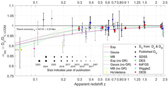
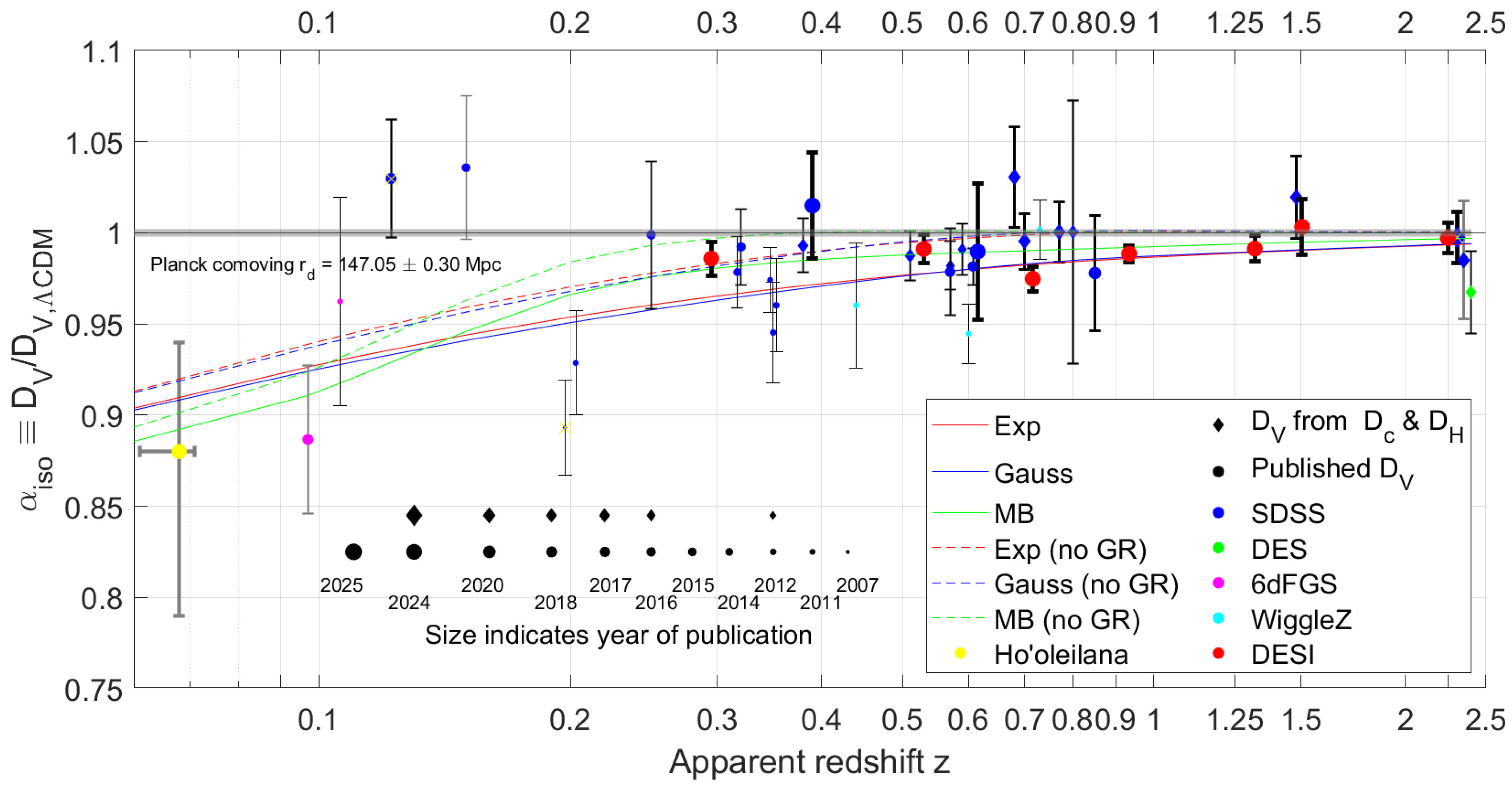
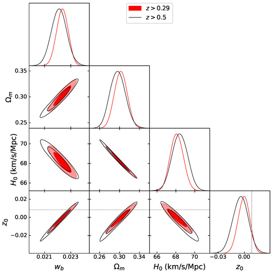
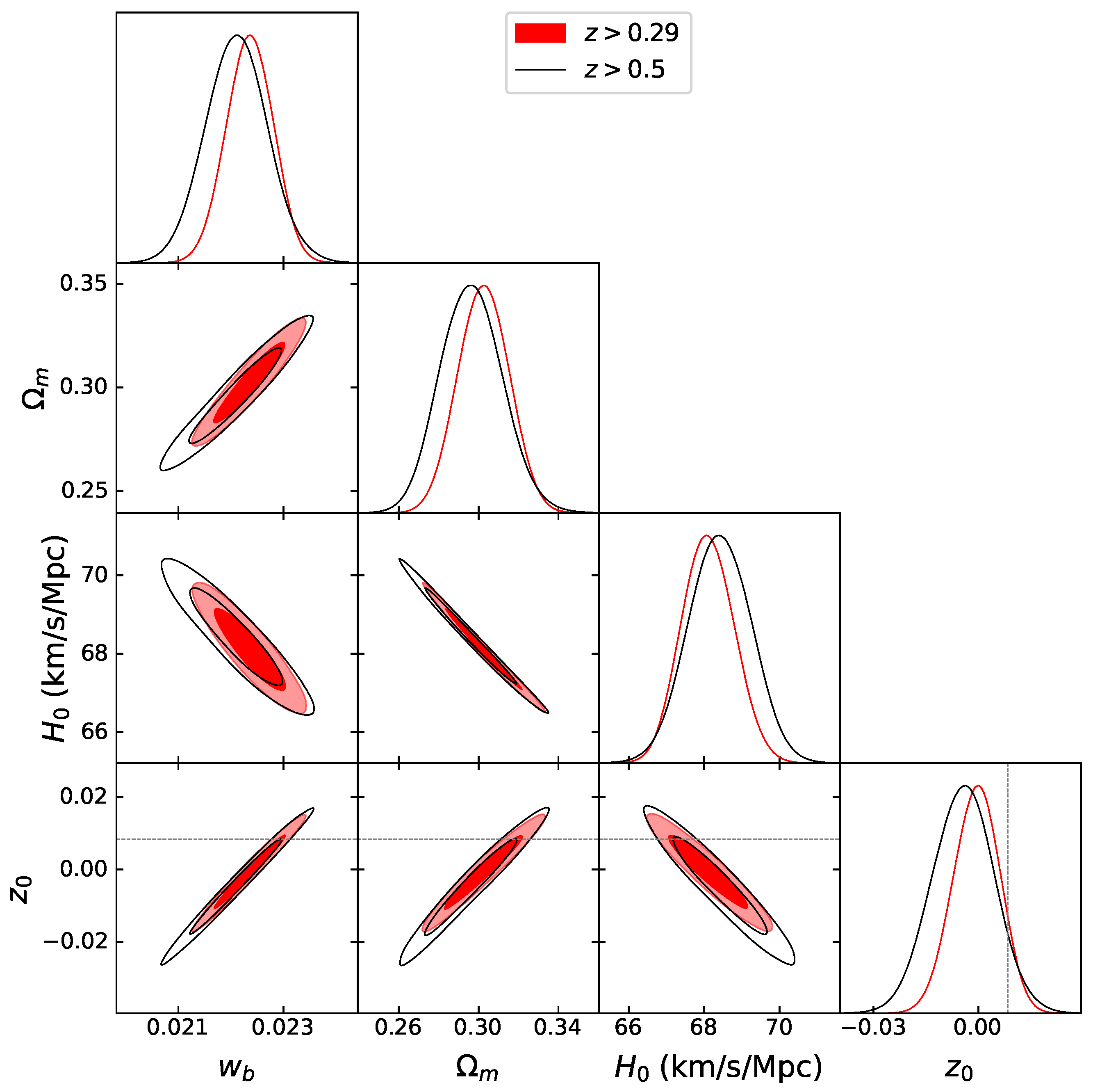
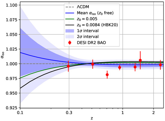
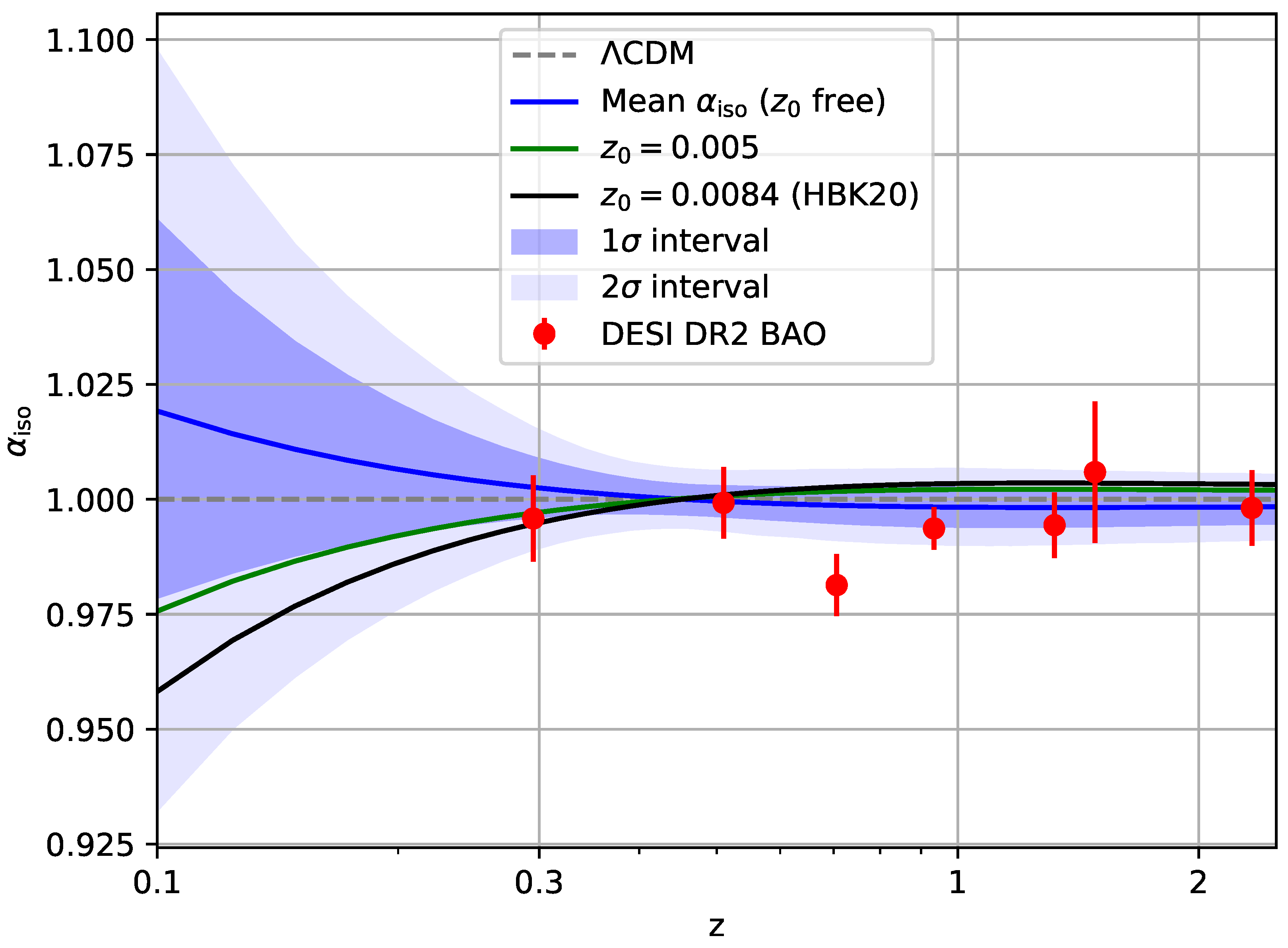
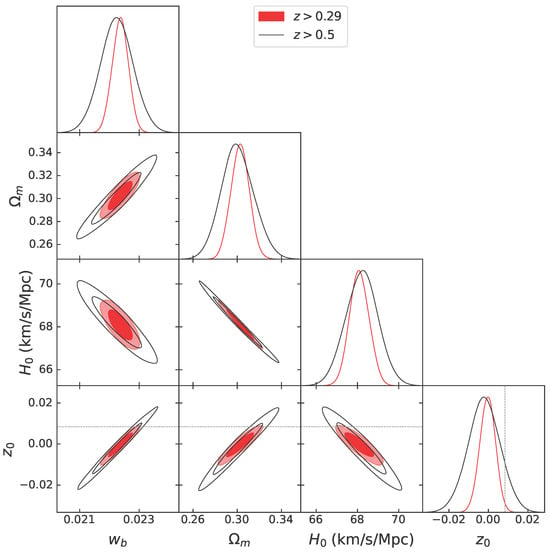
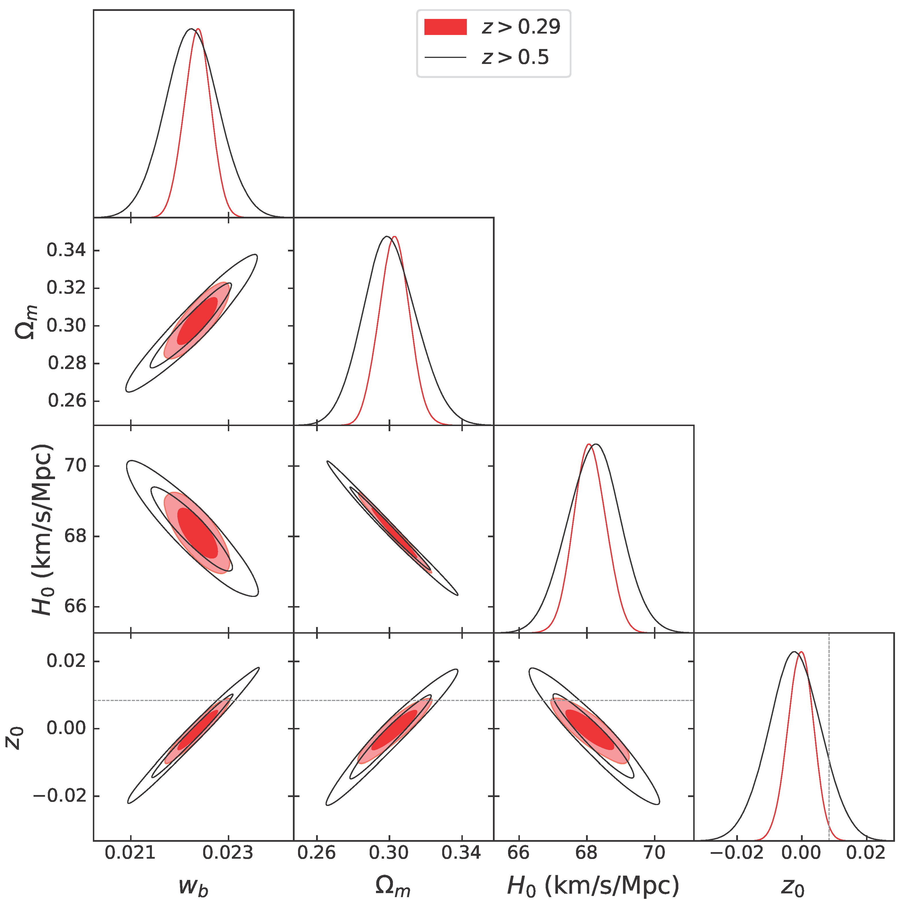

Disclaimer/Publisher’s Note: The statements, opinions and data contained in all publications are solely those of the individual author(s) and contributor(s) and not of MDPI and/or the editor(s). MDPI and/or the editor(s) disclaim responsibility for any injury to people or property resulting from any ideas, methods, instructions or products referred to in the content. |
© 2026 by the authors. Licensee MDPI, Basel, Switzerland. This article is an open access article distributed under the terms and conditions of the Creative Commons Attribution (CC BY) license.