Astrometric Systematic Errors as a Limiting Factor in Stellar-Aberration-Based Autonomous Navigation

Abstract

Stellar-aberration-based navigation requires angular measurements at the milliarcsecond (mas) level. While random sensor noise can be reduced by temporal integration, plate-solution uncertainty and residual geometric distortion may set a practical astrometric error floor. Here, we quantify the plate-model contribution to this error budget and examine its impact on the feasibility of stellar-aberration-based navigation. Using Gaia DR3 stars, HEALPix all-sky sampling, and covariance propagation to epoch J2026.0, we evaluate nine polynomial plate models while accounting for reference-star density and spatial distribution. We identify a bias–variance trade-off between model complexity, distortion-correction capability, and numerical stability. For the adopted ∼1° sparse-field configuration, the four-parameter linear model gives the lowest plate-constant variance, with a median of 0.95 mas and a 95th percentile of 1.7 mas. Using the first-order scaling of $\delta v\sim c\delta \theta$, this uncertainty corresponds to an approximate velocity-error scale of 0.9–2.5 m/s. These results show that plate-model errors can contribute at the meter-per-second level and must be included explicitly in StarNAV filter design.

1. Introduction

Autonomous onboard navigation is increasingly important for deep-space missions, where long communication delays and limited ground-tracking availability can constrain real-time operations [1,2]. Ground-based radiometric tracking remains indispensable, but its reliance on long-distance communication links and shared tracking resources can limit real-time autonomous operations. Consequently, autonomous celestial navigation techniques that reduce dependence on ground support have become an important research direction. Representative approaches include X-ray pulsar navigation (XNAV) [3] and image-based optical navigation, which has been used in several deep-space mission phases [4].

A notable flight demonstration is Deep Space 1, whose AutoNav system performed interplanetary cruise-orbit determination using images of distant asteroids acquired with the Miniature Integrated Camera and Spectrometer (MICAS) [5]. Optical navigation measurements have also been used in missions such as Stardust [6] and New Horizons [7], where onboard images of target bodies against stellar backgrounds supported trajectory refinement and encounter targeting, although these operations generally involved ground-based navigation processing. Beyond image-based navigation, the CHASE/Xihe mission carried the Solar Atomic Frequency Discriminator for Autonomous Navigation (SAFDAN), which demonstrated solar spectral velocity measurements in orbit and thereby provided an experimental basis for Doppler-velocity-based autonomous navigation [8].

A complementary approach is stellar-aberration-based navigation, which infers spacecraft velocity from velocity-induced changes in the apparent angular separations between stars. This concept was formalized as StarNAV by Christian et al. [9], and subsequent studies have examined its feasibility, observability, and integration with other navigation observables, e.g., [10,11]. Compared with navigation methods that rely on specific solar-system bodies, StarNAV is attractive because stellar sources are widely distributed across the sky and, with appropriate measurement geometry, can provide direct velocity information. Crucially, differential inter-star angle measurements can mitigate common-mode attitude errors, making the approach less dependent on absolute pointing knowledge. The availability of dense, high-precision stellar catalogs from the Gaia mission, particularly Gaia Data Release 3, further strengthens the practical basis for such measurements [12,13]. Recent studies have further explored wide-field sensor architectures, integrated navigation schemes, and adaptive filtering strategies to improve robustness and estimation accuracy [11,14].

However, practical StarNAV performance depends on the recovery of stellar directions or inter-star angles at the milliarcsecond level. At this precision, the astrometric reduction pipeline—including centroiding, geometric-distortion calibration, plate transformation, and reference-catalog errors—can introduce systematic errors that are comparable to the navigation signal. If not properly modeled, these errors may form a practical accuracy floor for the navigation system.

To assess one key component of the StarNAV error budget, this paper quantifies plate-model-induced systematic errors and examines how they depend on model complexity, reference-star density, and catalog precision. The remainder of this paper is organized as follows. Section 2 elaborates on the theoretical basis of StarNAV and defines the astrometric challenges specific to the single-field observation mode. Section 3 details the simulation methodology, including the construction of the high-precision navigation star catalog and the mathematical model for error propagation. Section 4 presents the results of the sensitivity analysis, evaluating the performance of nine plate models under varying star densities. Finally, Section 5 discusses the engineering implications of these findings, and Section 6 summarizes our conclusions.

2. Motivation

The fundamental observable in StarNAV is the velocity-induced change in the apparent angular separation between stars, arising from stellar aberration with respect to the inertial reference frame. To the first order, the characteristic aberration angle is of order $v/c$, where c is the speed of light. As an order-of-magnitude estimate, the corresponding velocity uncertainty scales as ${\sigma }_v\sim c{\sigma }_{\theta }$ before accounting for measurement geometry, weighting, and the number of available star pairs. Thus, 1 mas ($4.85\times {10}^{-9}$ rad) corresponds nominally to about 1.45 m/s. This scaling imposes a stringent requirement: m/s-level velocity estimation requires the astrometric error budget, including both random and systematic components, to be controlled at the milliarcsecond level.

In designing the observation scheme, we focus on a single-field mode that uses one sensor with a wide field of view (FOV). Compared with multi-field configurations [9], a single-field design is potentially attractive because of its simpler hardware architecture and lower mass and power requirements. However, such a configuration also introduces field-dependent astrometric distortions, especially toward the edge of the FOV. In a single-field design, all stellar measurements are reduced through a common focal plane-to-tangent plane transformation, so any inadequacy of the plate model directly propagates into the recovered inter-star angles. The raw optical distortions can be much larger than the milliarcsecond-level differential aberration signal and must therefore be calibrated through an appropriate plate model. Therefore, quantifying residual errors after plate-model calibration is essential for determining whether a single-field StarNAV system can meet the required astrometric precision.

To assess this source of error, it is useful to distinguish random measurement noise from systematic astrometric biases. When the random and systematic components are statistically characterized and treated as independent, the total positional uncertainty may be expressed in a root-sum-square (RSS) form. Random errors (${\sigma }_{\mathrm{rnd}}$) such as photon noise and detector readout noise can be reduced by increasing the exposure time or stacking multiple frames, approximately following statistical averaging under stable observing conditions. By contrast, biases associated with calibration, catalog errors, and plate-model inadequacy do not average down in the same way. After sufficient averaging, the remaining error budget may become dominated by systematic components (${\sigma }_{\mathrm{sys}}$), including calibration residuals and plate-model errors.

Conventional star-tracker attitude performance is commonly specified at the arcsecond level, which illustrates the gap between attitude sensing and the milliarcsecond-level astrometric precision required here. However, system-level attitude performance should not be directly equated with the precision of stellar angular measurements. One important detector-level contributor is systematic centroiding error on the focal plane. For instance, the Center of Gravity (COG) method is known to suffer from periodic sub-pixel “S-curve” errors, whose reported magnitude can reach the level of several hundredths of a pixel [15]. Advanced centroiding algorithms such as Fast Gaussian Fitting and sieve-search-based approaches can substantially reduce centroiding errors [16,17]. Nevertheless, if detector-level systematic centroiding biases are not calibrated, they may remain at the level of several hundredths of a pixel [18]. In this study, centroiding errors are not the main object of investigation; they are introduced only to illustrate the severity of the measurement requirement. The following analysis isolates the plate-model contribution by assuming that detector-level centroiding has been calibrated or treated separately.

In this work, we adopt a representative 1° × 1° FOV as the fiducial single-field configuration. This choice reflects a trade-off between reference-star availability and distortion control. A smaller FOV may contain too few reference stars for an overdetermined plate solution, whereas a larger FOV generally increases the importance of higher-order distortion terms. The required number of reference stars depends on the number of plate constants; in practice, an overdetermined solution requires more stars than the mathematical minimum. For a 1° field sampled by a $1024\times 1024$ detector, the pixel scale is approximately ${3.52}^{″}$ per pixel. We use 200 mas as an order-of-magnitude diagnostic threshold for catastrophic plate-solution failure in Section 4.3. For this pixel scale, 200 mas corresponds to about 0.057 pixels (≃0.06 pixel), which is comparable to the systematic centroiding biases of several hundredths of a pixel reported for uncalibrated or algorithm-dependent star-centroid measurements [15,18]. This comparison illustrates that a detector-level systematic bias of a size already familiar in the centroiding literature would be far above the nominal 1 mas StarNAV requirement if left uncalibrated.

Under a given plate model, reference-star distribution, and catalog precision, the residual systematic error after plate correction represents a practical lower bound on the attainable astrometric precision. In the context of StarNAV, this systematic component is driven by both reference-catalog uncertainties and residual errors in the plate transformation between detector coordinates and tangent-plane coordinates. Therefore, quantifying this component of ${\sigma }_{\mathrm{sys}}$ is essential for the separation of the astrometric-reduction floor from detector-level noise and centroiding performance.

The Gaia astrometric catalog provides the natural reference frame for this task because of its dense all-sky coverage and high-precision stellar astrometry [12,13]. Gaia Data Release 3 (DR3) provides sub-milliarcsecond astrometry for bright stars at the catalog epoch, but the propagated accuracy at future navigation epochs depends on proper-motion uncertainties and must be evaluated for the selected navigation-star sample [13]. For the bright-star subset considered in this study, the propagated Gaia positional uncertainties are expected to be below or comparable to the nominal 1 mas requirement, provided that proper-motion uncertainties are properly accounted for, as evaluated in Section 3.1. However, transferring catalog-level precision to measured focal-plane positions, then to recovered tangent-plane coordinates, is non-trivial. In this work, a plate-constant model is used to describe the transformation between measured focal-plane coordinates $(x,y)$ and standard tangent-plane coordinates $(\xi ,\eta )$. Although such transformations are standard in astrometry, the estimated plate constants have finite uncertainties because they are constrained by a limited number of reference stars with non-zero catalog errors. These uncertainties propagate into the corrected target-star position as a plate-solution variance contribution, commonly discussed as plate-constant variance [19].

Although plate-constant variance has been studied in classical photographic and wide-field astrometry [19,20,21], its impact on a milliarcsecond-level StarNAV error budget has not yet been systematically quantified. Building on the StarNAV measurement framework of Christian et al. [9], this work isolates the plate-model contribution to the astrometric error budget. Rather than modeling a complete hardware error budget, we isolate the plate-model contribution under controlled assumptions. By establishing a plate-model systematic error budget, we aim to quantify how plate-solution residuals constrain the attainable accuracy of stellar-aberration-based navigation.

3. Materials and Methods

3.1. Reference Catalog and Optical Geometry

We constructed a simulation framework to quantify plate-model-induced systematic errors. We adopted Gaia Data Release 3 (DR3) as the base catalog [13]. We selected stars with $G<10$ mag as candidate navigation stars, where G denotes the broad white-light Gaia magnitude measured over an approximately 330–1050 nm passband [12,13]. This threshold represents a bright-star sample relevant to high-sensitivity spaceborne optical sensors [11]. This magnitude cutoff favors high-SNR centroiding and keeps the catalog size manageable; its engineering implications are discussed in Section 5. This selection yielded 477,502 stars, corresponding to a mean density of about 12 stars deg⁻².

To sample regions with different stellar densities, we divided the sky using the Hierarchical Equal Area isoLatitude Pixelization (HEALPix) scheme [22]. We adopted a resolution parameter of $N_{\mathrm{side}}=64$ (order $k=6$). This partition divides the full sky into $12N_{\mathrm{side}}^2=\mathrm{49,152}$ equal-area pixels. The solid angle of each pixel is

$${\Omega }_{\mathrm{pix}}={\displaystyle \frac{4\pi }{12N_{\mathrm{side}}^2}}\simeq 0.84{\mathrm{deg}}^2,$$

(1)

corresponding to an effective linear scale of $\sqrt{{\Omega }_{\mathrm{pix}}}\simeq 0.92°$. This scale approximates the adopted 1° × 1° single-field FOV and provides a practical compromise between reference-star availability and distortion control. With the $G<10$ mag selection, the median field contains about eight stars, although the number varies strongly with Galactic latitude. This provides an overdetermined solution for simple plate models and allows sparse-field limitations to be assessed for higher-order models. The exact minimum number of stars depends on the number of plate constants in the model, and robust estimation generally requires more stars than the algebraic minimum. In our simulation, each HEALPix pixel is treated as an independent observational FOV.

The Gaia astrometric reference epoch is $t_0=\mathrm{J}2016.0$. For a representative mission epoch of $t=\mathrm{J}2026.0$, we propagated the catalog positions from J2016.0 using proper motions. In this simplified simulation, parallax and radial-velocity terms were neglected; their impact should be assessed in a full end-to-end navigation model. We adopted the standard astrometric propagation model described by Lindegren et al. [23] to derive the celestial coordinates and their associated covariance matrix at the mission epoch. We used the semi-major axis of the propagated tangent-plane error ellipse as the scalar positional uncertainty:

$${\sigma }_{\mathrm{pos},max}=\sqrt{\frac{1}{2}(C_{00}+C_{11})+\frac{1}{2}\sqrt{{(C_{11}-C_{00})}^2+4C_{01}^2}},$$

(2)

where $C_{00}$, $C_{11}$, and $C_{01}$ are the elements of the propagated tangent-plane covariance matrix.

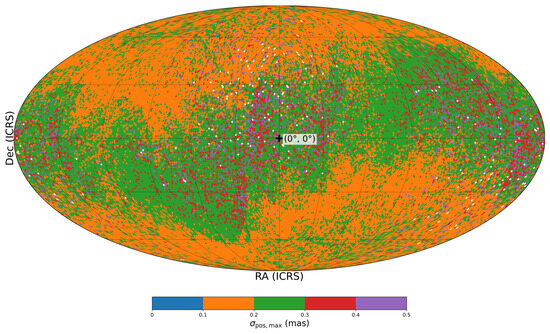
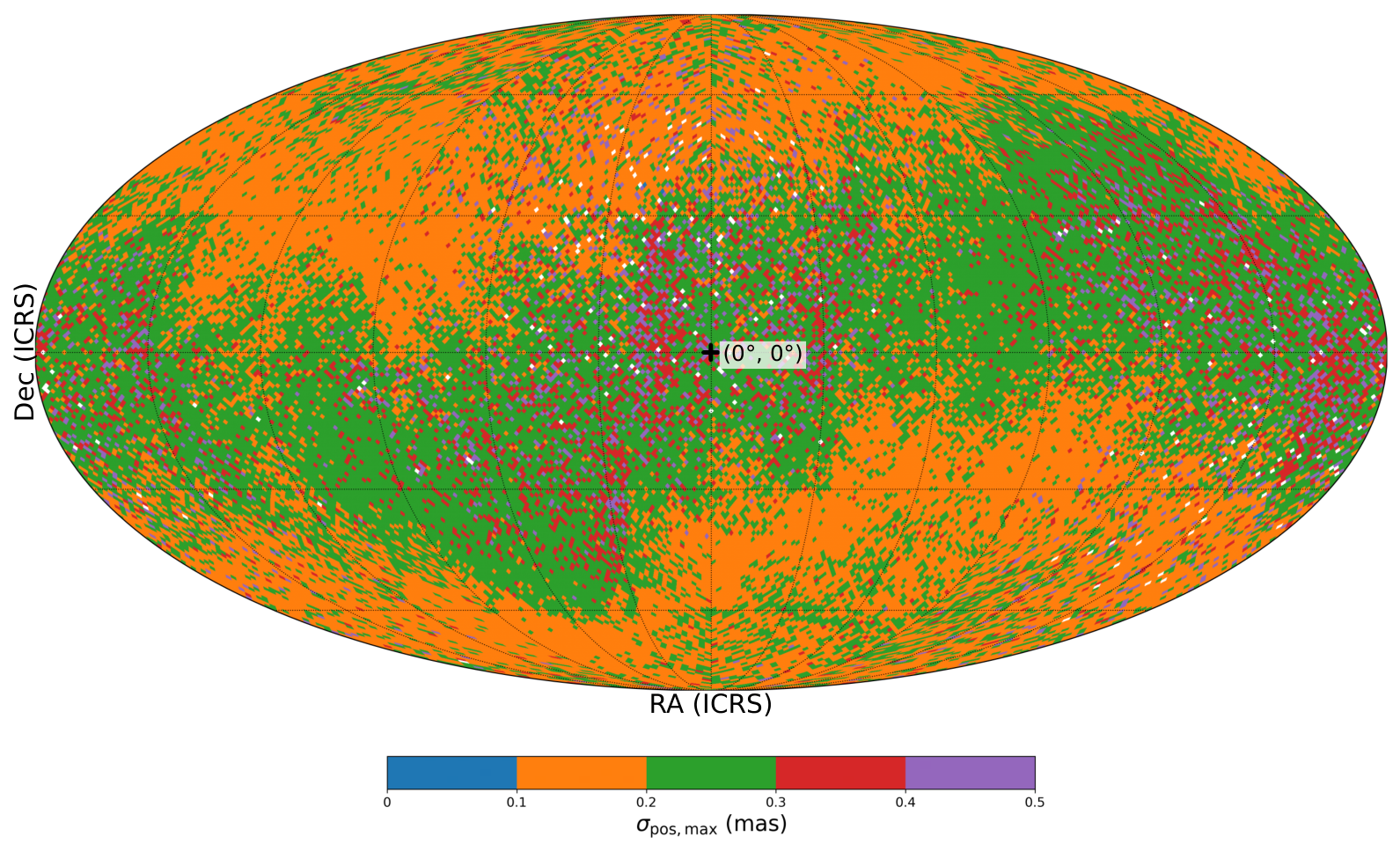
Figure 1 illustrates the all-sky distribution of these positional uncertainties. Most selected stars have propagated positional uncertainties below 0.3 mas at J2026.0, which is lower than the nominal 1 mas requirement.

Figure 1. All-sky distribution of the total positional uncertainty (${\sigma }_{\mathrm{pos},max}$) for navigation stars ($G<10$ mag) propagated to J2026.0. The color scale shows the median value in each HEALPix pixel and is clipped at 0.5 mas to emphasize the main distribution. The map is shown in a Mollweide all-sky projection in ICRS equatorial coordinates (RA–Dec), with $(\mathrm{RA},\mathrm{Dec})=(0°,0°)$ at the center of the map.

3.2. Plate-Model Formalism and Error Propagation

In an optical system, the mapping between focal-plane coordinates $(x,y)$ and tangent-plane coordinates $(\xi ,\eta )$ departs from an ideal linear transformation because of geometric distortion. Therefore, a plate model is used to describe this transformation. To compare plate-model choices for StarNAV, we considered a set of polynomial transformations, including both constrained and unconstrained forms. As a reference, a full two-dimensional polynomial of order n can be written as

$$\xi ={\displaystyle \sum _{i=0}^n}{\displaystyle \sum _{j=0}^{n-i}}{a}_{ij}{x}^i{y}^j,\eta ={\displaystyle \sum _{i=0}^n}{\displaystyle \sum _{j=0}^{n-i}}{b}_{ij}{x}^i{y}^j,$$

(3)

where n is the order of the polynomial [19]. The specific constrained and unconstrained models tested here are listed in Appendix A. In brief, we tested nine plate models with 4 to 14 parameters, ranging from conformal linear transformations to third-order radial-distortion models.

Higher-order models can fit more complex distortions, but they require more reference stars and are more sensitive to the spatial distribution and noise of those stars. For example, a fourth-order polynomial with 30 parameters has a formal minimum of 15 reference stars, but a stable weighted least-squares solution generally requires a substantially larger and well-distributed reference-star sample. In the sparse-field regime considered here, such models may become underdetermined or poorly conditioned. Consequently, the primary challenge is to identify a plate model (typically, of first or second order) that remains algebraically solvable and numerically stable under sparse star-count constraints.

To generate synthetic data with controlled distortion, we defined a reference truth model motivated by calibrated space-based optical instruments. The HST/ACS calibration is used only to motivate the order of magnitude of geometric-distortion amplitudes, not to define the physical pixel scale or exact optical geometry of the simulated StarNAV sensor [24]. Because the simulated StarNAV sensor has a much wider FOV than ACS/WFC, the adopted coefficients are not intended to reproduce the ACS/WFC solution. All detector coordinates are normalized over the simulated field before applying the plate model, and the residuals are converted to angular units using the adopted 1° field scale. The baseline linear coefficients used in the controlled distortion field are expressed as follows:

$$\begin{array}{cccccc}\hfill A& =0.9998,\hfill & \hfill B& =-0.0003,\hfill & \hfill C& =0.12945,\hfill \\ \hfill A^{\prime }& =0.0003,\hfill & \hfill B^{\prime }& =0.9998,\hfill & \hfill C^{\prime }& =-0.71780.\hfill \end{array}$$

(4)

We then added controlled second- and third-order terms to test the sensitivity of each fitted plate model to unmodelled distortion. The representative dimensionless coefficients, defined for normalized detector coordinates, were set as follows:

$$\begin{array}{c}p=q=r=1.0\times {10}^{-4},\hfill \\ p^{\prime }=r^{\prime }=1.0\times {10}^{-4},q^{\prime }=-1.0\times {10}^{-4},\hfill \\ \alpha ={\alpha }^{\prime }=1.0\times {10}^{-7}.\hfill \end{array}$$

(5)

We then propagated reference-star uncertainties through each plate solution. In this paper, we separate the variance caused by noisy reference stars from the bias caused by model inadequacy. The former is the plate-constant-variance (PCV) contribution, while the latter is the residual distortion left when the fitted plate model cannot represent the reference truth model. For each HEALPix field, the observation equation for a given plate model can be written as

$$\mathbf{y}=\mathbf{H}\mathbf{p}+ϵ,$$

(6)

where $\mathbf{y}={[{\xi }_1,{\eta }_1,{\xi }_2,{\eta }_2,\dots ,{\xi }_N,{\eta }_N]}^{\mathsf{T}}$ aggregates the standard coordinates of the N reference stars and $\mathbf{p}$ is the vector of plate constants. For each plate model, the design matrix ($\mathbf{H}\in {\mathbb{R}}^{2N\times M}$) is constructed from the corresponding basis functions listed in Table A1. For example, for the six-constant affine model, $\mathbf{H}$ is

$$\mathbf{H}=\left[\begin{array}{cccccc}{x}_1& y_1& 1& 0& 0& 0\\ 0& 0& 0& x_1& y_1& 1\\ ⋮& ⋮& ⋮& ⋮& ⋮& ⋮\\ x_N& y_N& 1& 0& 0& 0\\ 0& 0& 0& x_N& y_N& 1\end{array}\right]$$

(7)

Plate constants are estimated by weighted least squares. The resulting covariance matrix of the parameters ($\mathrm{Cov}\left(\mathbf{p}\right)$) is given by

$$\mathrm{Cov}\left(\mathbf{p}\right)={\left({\mathbf{H}}^{\mathsf{T}}\mathbf{W}\mathbf{H}\right)}^{-1}.$$

(8)

Here, $\mathbf{W}={\mathbf{C}}_y^{-1}$, where ${\mathbf{C}}_y$ is the covariance matrix of the standard-coordinate observations after propagating catalog and centroiding uncertainties into the same coordinate system. For a navigation-target star at a measured location $(x_t,y_t)$, let ${\mathbf{H}}_t\in {\mathbb{R}}^{2\times M}$ be the target design matrix constructed from the same model basis. The PCV contribution to the corrected target-star coordinates is then

$${\mathbf{C}}_{t,\mathrm{pcv}}\approx {\mathbf{H}}_t\mathrm{Cov}\left(\mathbf{p}\right){\mathbf{H}}_t^{\mathsf{T}}.$$

(9)

We define the scalar plate-constant-variance error as

$${\sigma }_{\mathrm{pcv}}=\sqrt{\mathrm{tr}\left({\mathbf{C}}_{t,\mathrm{pcv}}\right)}.$$

(10)

This metric quantifies the uncertainty in the target-star direction caused by the propagation of reference-star errors through the plate solution. If the residual model bias (${\mathbf{b}}_{t,\mathrm{mod}}$) is explicitly evaluated against the reference truth model, the total plate-model error can be represented as

$${\sigma }_{\mathrm{plate}}=\sqrt{{\sigma }_{\mathrm{pcv}}^2+{\parallel {\mathbf{b}}_{t,\mathrm{mod}}\parallel }^2}.$$

(11)

Unless otherwise stated, the numerical results below report the PCV contribution (${\sigma }_{\mathrm{pcv}}$) and use the reference truth model only to test sensitivity to model inadequacy.

4. Results

4.1. Spatial Error Distribution in a Fiducial Sparse Field

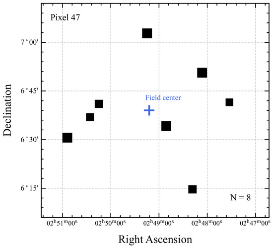
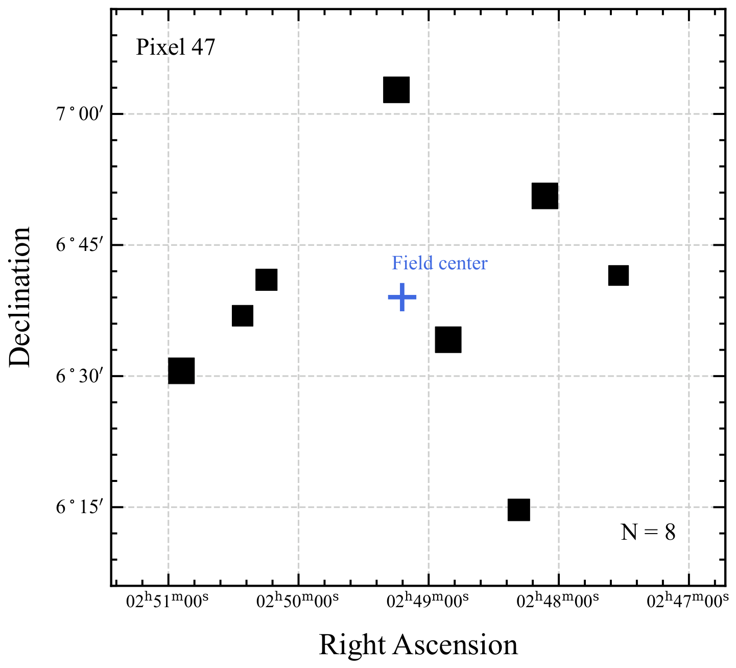
To illustrate the impact of plate-model selection on astrometric accuracy, we selected a fiducial HEALPix field (Pixel 47) containing eight reference stars. This number corresponds to the median star count in our all-sky sample for the adopted $G<10$ mag selection and ∼1° field scale. Figure 2 shows the spatial distribution of these reference stars within the field. The sparse and irregular distribution illustrates the limited geometric constraints that can occur in median-density fields. We use this field to compare the nine plate models.

Figure 2. Distribution of the eight reference stars in the selected fiducial field (Pixel 47). Black squares mark the reference stars, and the blue cross marks the geometric field center.

Following Section 3.2, we report the plate-constant-variance error (${\sigma }_{\mathrm{pcv}}$) as the propagated positional uncertainty derived from the covariance of the fitted plate constants. At a given focal-plane position, this scalar uncertainty is computed from the two-dimensional propagated covariance as

$${\sigma }_{\mathrm{pcv}}=\sqrt{\mathrm{tr}\left({\mathbf{H}}_t\mathrm{Cov}\left(\mathbf{p}\right){\mathbf{H}}_t^{\mathsf{T}}\right)}.$$

(12)

This metric excludes the centroiding noise of the target star itself but includes the uncertainty propagated from the reference stars through the plate solution.

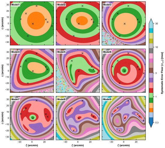
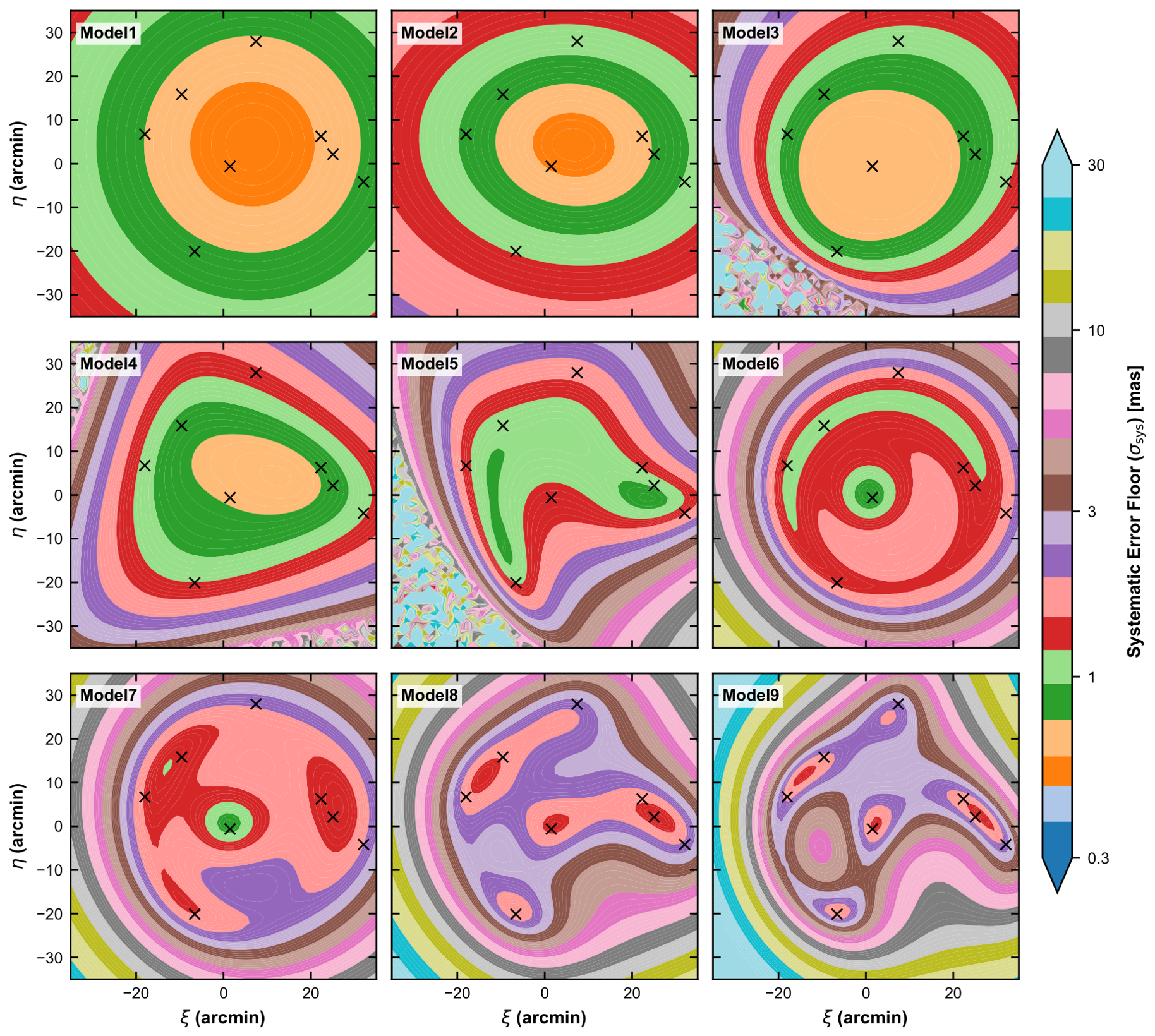
Figure 3 shows the spatial distribution of ${\sigma }_{\mathrm{pcv}}$ across the sensor plane. The models show clear differences in their error patterns. Linear models (Models 1–2) show smooth error distributions, with ${\sigma }_{\mathrm{pcv}}$ remaining below 2 mas across the field. This low variance does not imply that linear models fully remove optical distortion; their model bias must be evaluated separately. In contrast, the high-parameter models (Models 8–9) become poorly conditioned in this low-star-count regime. Owing to weak geometric constraints, the propagated error increases rapidly toward the FOV periphery and exceeds 20 mas in some regions. This edge amplification is analogous to the Runge phenomenon, but in the present case, it is more directly caused by poor conditioning and sparse boundary constraints.

Figure 3. Spatial distribution of the plate-constant-variance error (${\sigma }_{\mathrm{pcv}}$) in the selected fiducial FOV (Pixel 47) containing eight reference stars.

This boundary instability is problematic for StarNAV because the method relies on relative astrometry across the field. Large angular separations between stellar pairs can improve aberration sensitivity, but they also require reliable astrometry over a large fraction of the FOV. For high-parameter models, the large uncertainties near the FOV corners imply that stellar pairs involving peripheral sources may suffer from amplified error propagation. As a result, the advantage of wide-separation stellar pairs may be reduced or lost if the plate model is not sufficiently constrained.

4.2. Dependence of Plate-Constant Variance on Star Density

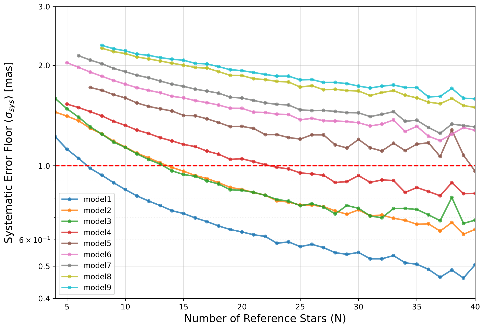
After illustrating the poor conditioning of high-parameter models in a sparse fiducial field, we quantified how the PCV error depends on the number of reference stars. We analyzed all 49,152 HEALPix fields. For each field and each model, we computed the maximum ${\sigma }_{\mathrm{pcv}}$ over the focal-plane grid, denoted as ${\sigma }_{max}$. Fields were then grouped by their reference-star count (N), and the median ${\sigma }_{max}$ was computed for each group.

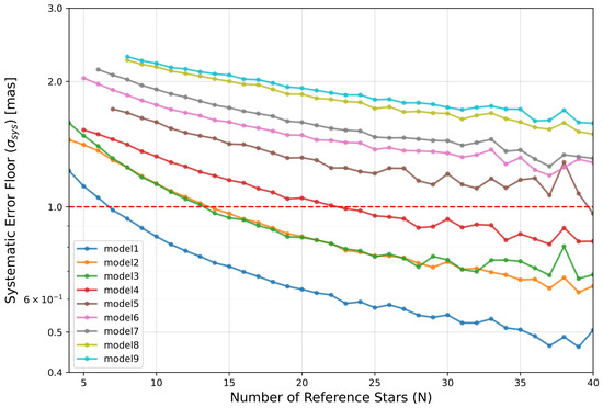
Figure 4 shows the dependence of $\mathrm{median}\left({\sigma }_{max}\right)$ on N for the nine models, illustrating the increasing sensitivity of high-parameter models to sparse reference-star geometry. Model 1 is the least demanding in terms of reference-star count, reaching the 1 mas threshold at $N=7$ in this median statistic. Models 2–3 require $N\simeq 14$ reference stars to reach the same threshold. Model 5 reaches the 1 mas threshold only at $N\simeq 40$, while Models 6–9 do not reach this threshold within the sampled star-count range. Because the median available star count is only $N\approx 8$, these high-parameter models are poorly suited to the median-density $G<10$ mag fields considered here. The corresponding reference-star count thresholds are summarized in Table 1.

Figure 4. Dependence of the median maximum plate-constant-variance error ($\mathrm{median}\left({\sigma }_{max}\right)$) on the number of reference stars (N). The red dashed horizontal line marks the nominal 1 mas target threshold.

Table 1. Reference-star count thresholds required for the median maximum plate-constant-variance error to fall below 10 mas and 1 mas. “N/A” indicates that the threshold is not reached within the sampled star-count range.

Model	${\mathit{N}}_{10\mathbf{mas}}$	${\mathit{N}}_{1\mathbf{mas}}$
Model 1 (Linear 4)	4	7
Model 2 (Linear 6)	4	14
Model 3 (Quad 6)	4	14
Model 4 (Quad 8)	5	23
Model 5 (Quad 12)	7	40
Model 6 (Cubic 7)	5	N/A
Model 7 (Cubic 9)	6	N/A
Model 8 (Cubic 13)	8	N/A
Model 9 (Cubic 14)	8	N/A

4.3. All-Sky Statistical Performance and Stability

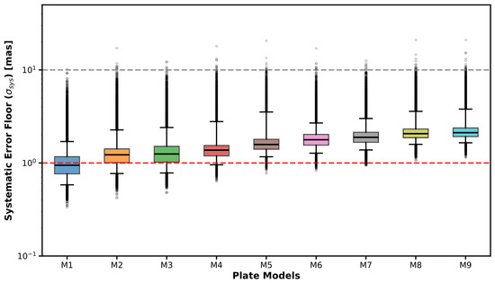
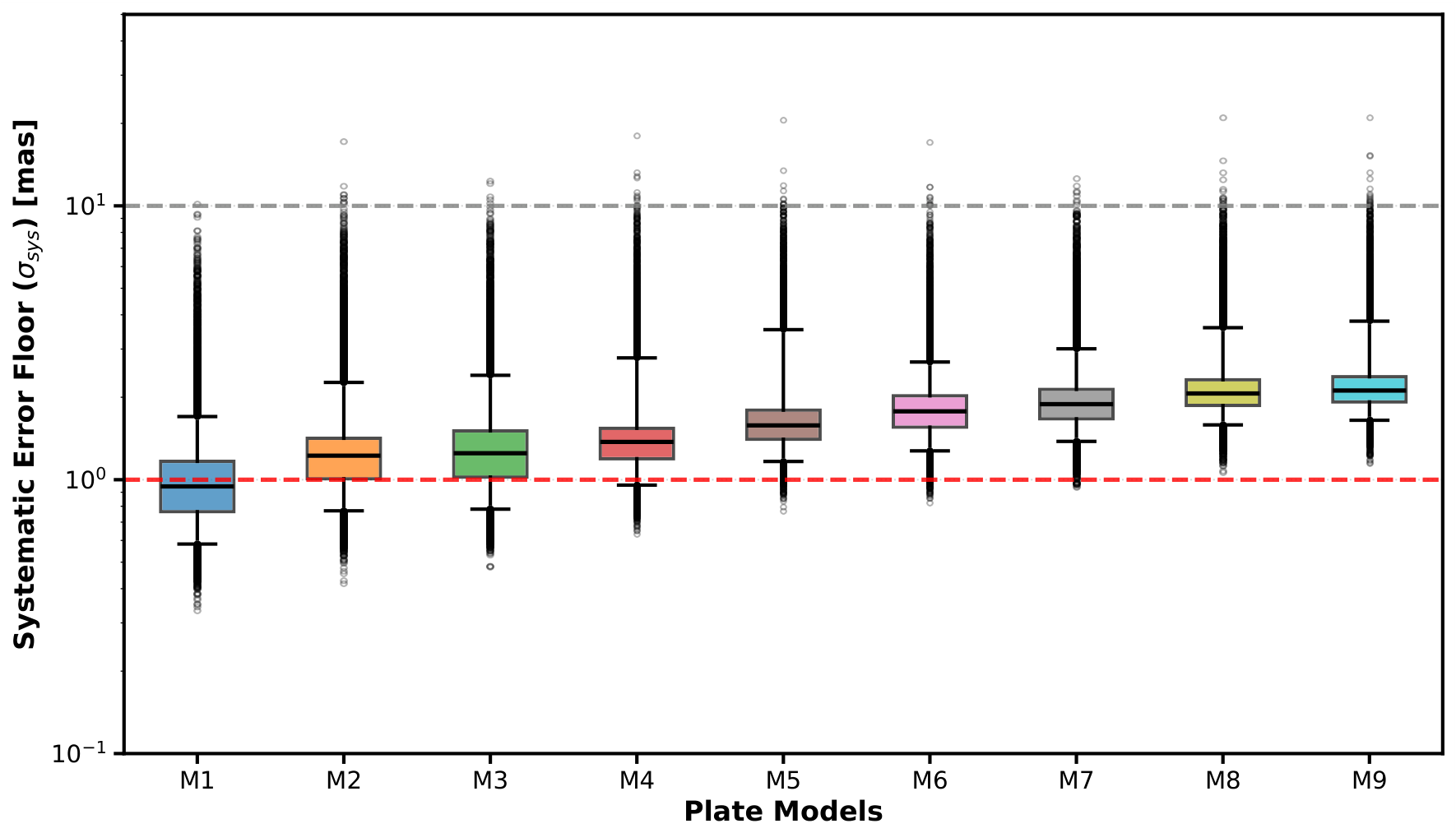
To assess the robustness of the plate solutions under all-sky sampling, we analyzed all 49,152 HEALPix fields. We defined a catastrophic plate-solution failure as any case with ${\sigma }_{\mathrm{pcv}}>200$ mas. This threshold is not a navigation requirement but a diagnostic criterion used to identify catastrophic instability. It is roughly two orders of magnitude above the nominal 1 mas target and usually indicates a nearly singular or poorly conditioned plate solution. Table 2 and Figure 5 summarize the results.

Table 2. Global performance statistics across all 49,152 HEALPix fields. The fail rate is the percentage of fields with catastrophic plate-solution instability, defined as ${\sigma }_{\mathrm{pcv}}>200$ mas. The 5th, 50th, and 95th percentiles are computed only from successful fields.

Model	P5 [mas]	P50 [mas]	P95 [mas]	Fail Rate [%]
Model 1	0.582	0.945	1.700	0.00
Model 2	0.770	1.224	2.266	0.00
Model 3	0.781	1.249	2.407	26.50
Model 4	0.956	1.374	2.785	12.95
Model 5	1.166	1.578	3.531	46.80
Model 6	1.274	1.777	2.690	0.00
Model 7	1.380	1.887	3.006	0.00
Model 8	1.585	2.065	3.591	0.00
Model 9	1.648	2.117	3.794	0.00

Figure 5. All-sky distribution of ${\sigma }_{\mathrm{pcv}}$ for the nine plate models. Failed fields are excluded from the box plot. The box shows the interquartile range (25th–75th percentiles).

The global analysis shows that some higher-parameter models have substantial reliability risks. Model 5 has the highest failure rate of 46.80%, indicating that it is unsuitable for autonomous use under the present $G<10$ mag, ∼1° FOV assumptions. Models 3 and 4 also show non-negligible failure rates of 26.5% and 13.0%, respectively.

In contrast, Model 1 is the most robust under this failure criterion. It remains below the failure threshold in all sky fields. It also has the lowest median ${\sigma }_{\mathrm{pcv}}$ of 0.95 mas among the tested models. Its 95th percentile is 1.70 mas, indicating that 95% of successful fields remain below this level.Because the quantiles are computed only from successful cases, they should be interpreted together with the failure rate.

The zero failure rates of Models 6–9 should not be interpreted as an overall advantage of the cubic models. The failure rate is controlled by rare cases with ${\sigma }_{\mathrm{pcv}}>200$ mas, whereas the listed percentiles describe the successful fields only. The non-zero failure rates of Models 3–5 indicate that, in some sparse and geometrically uneven fields, the quadratic inversion can become locally ill-conditioned and produce catastrophic uncertainty amplification. Models 6–9 add constrained radial-cubic terms such as $\alpha x{r}^2$ and $\alpha y{r}^2$, which, in the present parameterization, suppress these extreme outliers, but their larger P50 and P95 values show that their typical variance remains higher. Thus, the zero failure rate reflects the absence of catastrophic outliers under this specific threshold, not the general superiority of the cubic models.

These statistics indicate that the four-parameter linear model (Model 1) provides the best trade-off in the present PCV analysis. This does not imply that Model 1 is optimal once residual model bias is included. With greater centroiding noise, high-parameter models would be even more sensitive to reference-star noise. Under the sparse-field conditions considered here, this sensitivity outweighs their potential advantage in modeling higher-order distortion.

Finally, we translate the plate-solution error into an approximate velocity-error scale. Using the first-order scaling ($\delta v\sim c\delta \theta$), the Model 1 range of 0.6–1.7 mas corresponds to an approximate velocity-error scale of 0.9–2.5 m/s, with a median of 1.4 m/s. This scaling suggests that plate-solution uncertainty alone can contribute an error scale of order 1 m/s, even if random measurement noise is reduced by temporal averaging. Therefore, this plate-model contribution should be included in the design and covariance modeling of future stellar-aberration-based navigation filters.

5. Discussion

This study evaluates the plate-model contribution to the astrometric error budget of stellar-aberration-based autonomous navigation. We now discuss the implications for optical architecture, plate-model selection, and StarNAV velocity-error estimates.

Optical configuration is a key design choice for stellar-aberration-based navigation. Our simulations focused on a single-field configuration with a ∼1° FOV because of its hardware simplicity. However, this configuration is sensitive to field-dependent distortion because useful reference and navigation stars may lie near the edge of the sensor, where distortion and plate-solution uncertainty are often larger. A multi-field architecture using two or more narrow-field telescopes pointed in different directions could reduce this problem by keeping each stellar image closer to the optical axis while still providing a large angular baseline. Although multi-field systems increase mass, volume, and power consumption, they may become attractive for missions requiring sub-milliarcsecond astrometric stability, especially if wide-field distortion cannot be calibrated to the required level.

The adopted magnitude cutoff of $G<10$ mag also deserves comment. This value should not be interpreted as a fundamental limit of stellar-aberration-based navigation but as a bright-star benchmark chosen to keep centroiding and Gaia proper-motion propagation in a high-SNR regime. Published small-satellite star-sensor examples commonly adopt shallower limiting magnitudes, such as $V\simeq 6.5$ for StarSense and StarberrySense [25,26]. In contrast, higher-sensitivity optical navigation or small-telescope concepts can use fainter stars when aperture, integration time, attitude stability, and onboard processing permit. For example, an 85 mm nanosatellite telescope concept was analyzed at 1 Hz using an 11th-magnitude guide star [27], while the New Horizons LORRI optical-navigation camera can detect much fainter unresolved targets through long exposures, pixel re-binning, special tracking, and image co-addition [28,29]. Taken together, these published instrument studies bracket the adopted limit: $G<10$ mag is deeper than the operating assumptions of many wide-field real-time star trackers but remains a plausible and conservative order of magnitude for a dedicated high-sensitivity navigation camera. Relaxing the limit to $G<11$ mag or $G<12$ mag would increase the number of reference stars per field and would likely reduce the conditioning and fail-rate problems found for higher-order plate models. The trade-off is that fainter-star operation generally requires longer integration, a larger aperture, improved tracking, or stacking, which reintroduce random-noise and operational constraints not modeled explicitly here. A full joint optimization of limiting magnitude, exposure strategy, aperture, and plate-model order is therefore left for future work.

Under the plate-constant-variance metric, our analysis identifies the four-parameter linear model (Model 1) as the most stable option for sparse fields with $N\approx 8$. However, this numerical stability comes at the cost of unmodeled optical distortion. Real optical systems generally contain field-dependent radial, tangential, and higher-order distortions. A purely linear model cannot absorb these nonlinear terms; instead, it leaves a residual distortion bias that is not captured by the plate-constant-variance term alone. Higher-order polynomials are commonly used in dense-field astrometry to model such distortions. In the sparse $G<10$ mag fields considered here, however, free estimation of many high-order coefficients is poorly constrained. The problem is not only the formal number of degrees of freedom but also the poor conditioning caused by uneven reference-star geometry. An alternative to general Cartesian polynomial expansions is to impose a more physically constrained distortion model. The Brown–Conrady family, originating from classical lens-decentering and photogrammetric camera calibration work [30,31] and widely used in modern camera calibration [32], combines radial distortion terms with tangential or decentering terms. Models 6–9 include a first-order radial component ($\alpha x{r}^2$, $\alpha y{r}^2$), but the models tested here do not include tangential/decentering terms or higher-order radial terms such as $r^4$ and $r^6$. Such physically constrained forms could, in principle, capture dominant optical distortion modes with fewer freely estimated coefficients than a general polynomial of comparable flexibility, thereby shifting the bias–variance trade-off toward better-conditioned solutions at low reference-star counts. We did not explore this model class in the present analysis; validating a Brown–Conrady-type model against a specific optical design is therefore a natural extension of the present plate-model comparison.

Therefore, the 0.6–1.7 mas range obtained for Model 1 should be interpreted as a low-variance benchmark, not as the complete plate-model error. A complete assessment must also include the residual bias from unmodelled distortion. This distinction is important in interpreting the apparent advantage of Model 1: it is stable in the covariance-propagation sense, but it may not be the physically best distortion-correction model if higher-order field distortion is significant. Therefore, future work should combine plate-solution variance, calibrated distortion priors, and residual model bias in a single astrometric error model.

Previous StarNAV analyses have often emphasized measurement geometry and random sensor noise while treating detailed astrometric-reduction errors as calibrated or secondary effects [9]. In such a framework, improved integration or repeated measurements primarily reduce the random component of the velocity error. Our results indicate that the astrometric-reduction component deserves explicit treatment in the StarNAV error budget. Using the first-order scaling ($\delta v\sim c\delta \theta$), the Model 1 median plate-solution uncertainty of ∼0.95 mas corresponds to an approximate velocity-error scale of ∼1.4 m/s. This estimate should be interpreted as the contribution of plate-solution uncertainty rather than as a lower bound on the full navigation solution. Therefore, future navigation filters should include plate-model uncertainty and residual distortion bias explicitly rather than treating all astrometric errors as independent random noise that averages down with integration time.

6. Conclusions

In this paper, we performed an all-sky sensitivity analysis of the plate-model contribution to the astrometric error budget in stellar-aberration-based navigation. Using Gaia DR3 stars, HEALPix all-sky sampling, and covariance propagation, we evaluated nine plate models under a representative sparse-field configuration. For the adopted ∼1° field scale and $G<10$ mag reference-star selection, the median number of available stars is only $N\approx 8$, making freely fitted high-parameter plate models poorly constrained or unstable. Under the plate-constant-variance metric, the four-parameter linear model is the most stable case, with a median error of 0.95 mas and a 95th percentile of 1.7 mas. However, this result reflects low variance and numerical robustness, not necessarily sufficient correction of real nonlinear optical distortion. Using the first-order scaling ($\delta v\sim c\delta \theta$), this plate-solution uncertainty corresponds to an approximate velocity-error scale of 0.9–2.5 m s⁻¹. These results support the feasibility of StarNAV only if plate-solution uncertainty and residual distortion bias are explicitly included in the navigation error budget. Therefore, future systems should treat the plate model as a key contributor to the astrometric error budget, alongside sensor noise, optical calibration, and catalog errors.

References

- Turan, E.; Speretta, S.; Gill, E. Autonomous navigation for deep space small satellites: Scientific and technological advances. Acta Astronaut. 2022, 193, 56–74. [Google Scholar] [CrossRef] [Scilit]
- McKee, P.; Kowalski, J.; Christian, J.A. Navigation and star identification for an interstellar mission. Acta Astronaut. 2022, 192, 390–401. [Google Scholar] [CrossRef] [Scilit]
- Sheikh, S.I.; Pines, D.J.; Ray, P.S.; Wood, K.S.; Lovellette, M.N.; Wolff, M.T. Spacecraft Navigation Using X-Ray Pulsars. J. Guid. Control Dyn. 2006, 29, 49–63. [Google Scholar] [CrossRef] [Scilit]
- Ma, Y.; Gu, C.; Jiang, J.; Wei, X.; Xie, D.; Wang, G.; Li, J. Review of Autonomous Optical Navigation for Deep Space Exploration. IEEE Trans. Instrum. Meas. 2025, 74, 8502430. [Google Scholar] [CrossRef] [Scilit]
- Bhaskaran, S. The Deep Space 1 Autonomous Navigation System—A Post-Flight Analysis. In Proceedings of the AIAA/AAS Astrodynamics Specialist Conference and Exhibit, Denver, CO, USA, 14–17 August 2000. [Google Scholar] [CrossRef] [Scilit]
- Bhaskaran, S.; Mastrodemos, N.; Riedel, J.E.; Synnott, S.P. Optical Navigation for the Stardust Wild 2 Encounter. In Proceedings of the 18th International Symposium on Space Flight Dynamics, Munich, Germany, 11–15 October 2004; Volume 548. [Google Scholar]
- Flanigan, S.H.; Rogers, G.D.; Guo, Y.; Kirk, M.N.; Weaver, H.A.; Owen, W.M.; Jackman, C.D.; Bauman, J.; Pelletier, F.; Nelson, D.; et al. Destination Pluto: New Horizons performance during the approach phase. Acta Astronaut. 2016, 128, 33–43. [Google Scholar] [CrossRef] [Scilit]
- Zhang, W.; Yang, Y.; You, W.; Zheng, J.; Ye, H.; Ji, K.; Chen, X.; Lin, X.; Huang, Q.; Cheng, X.; et al. Autonomous navigation method and technology implementation of high-precision solar spectral velocity measurement. Sci. China Phys. Mech. Astron. 2022, 65, 289606. [Google Scholar] [CrossRef] [Scilit]
- Christian, J.A. StarNAV: Autonomous Optical Navigation of a Spacecraft by the Relativistic Perturbation of Starlight. Sensors 2019, 19, 4064. [Google Scholar] [CrossRef] [Scilit] [PubMed]
- Li, M.; Sun, J.; Peng, Y.; Liu, J. Observability and Performance Analysis of Spacecraft Autonomous Navigation Using Stellar Aberration Observation. In Proceedings of the 2021 5th International Conference on Vision, Image and Signal Processing (ICVISP), Kuala Lumpur, Malaysia, 18–20 December 2021; IEEE: Piscataway, NJ, USA, 2021; pp. 218–223. [Google Scholar] [CrossRef] [Scilit]
- Xiong, K.; Wei, C.; Zhou, P. Integrated Autonomous Optical Navigation Using Q-Learning Extended Kalman Filter. Aircr. Eng. Aerosp. Technol. 2022, 94, 848–861. [Google Scholar] [CrossRef] [Scilit]
- Gaia Collaboration; Prusti, T.; de Bruijne, J.H.J.; Brown, A.G.A.; Vallenari, A.; Babusiaux, C.; Bailer-Jones, C.A.L.; Bastian, U.; Biermann, M.; Evans, D.W.; et al. The Gaia mission. Astron. Astrophys. 2016, 595, A1. [Google Scholar] [CrossRef] [Scilit]
- Vallenari, A. et al. [Gaia Collaboration] Gaia Data Release 3. Summary of the content and survey properties. Astron. Astrophys. 2023, 674, A1. [Google Scholar] [CrossRef] [Scilit]
- McKee, P.; Nguyen, H.; Kudenov, M.W.; Christian, J.A. StarNAV with a wide field-of-view optical sensor. Acta Astronaut. 2022, 197, 220–234. [Google Scholar] [CrossRef] [Scilit]
- Wei, X.; Xu, J.; Li, J.; Yan, J.; Zhang, G. S-curve centroiding error correction for star sensor. Acta Astronaut. 2014, 99, 231–241. [Google Scholar] [CrossRef] [Scilit]
- Wan, X.; Wang, G.; Wei, X.; Li, J.; Zhang, G. Star Centroiding Based on Fast Gaussian Fitting for Star Sensors. Sensors 2018, 18, 2836. [Google Scholar] [CrossRef] [Scilit] [PubMed]
- Karaparambil, V.C.; Manjarekar, N.S.; Singru, P.M. Sieve Search Centroiding Algorithm for Star Sensors. Sensors 2023, 23, 3222. [Google Scholar] [CrossRef] [Scilit] [PubMed]
- Yang, J.; Liang, B.; Zhang, T.; Song, J. A Novel Systematic Error Compensation Algorithm Based on Least Squares Support Vector Regression for Star Sensor Image Centroid Estimation. Sensors 2011, 11, 7341–7363. [Google Scholar] [CrossRef] [Scilit] [PubMed]
- Eichhorn, H.; Williams, C.A. On the systematic accuracy of photographic astrographic data. Astron. J. 1963, 68, 221–231. [Google Scholar] [CrossRef] [Scilit] [PubMed]
- Plummer, H.C. Note on the Influence of the Plate Constants on the Accuracy of the Position of an Object measured on a Photograph. Mon. Not. R. Astron. Soc. 1904, 64, 645. [Google Scholar] [CrossRef] [Scilit]
- Bienayme, O. Field astrometry using orthogonal functions. Astron. Astrophys. 1993, 278, 301–306. [Google Scholar]
- Górski, K.M.; Hivon, E.; Banday, A.J.; Wandelt, B.D.; Hansen, F.K.; Reinecke, M.; Bartelmann, M. HEALPix: A Framework for High-Resolution Discretization and Fast Analysis of Data Distributed on the Sphere. Astrophys. J. 2005, 622, 759–771. [Google Scholar] [CrossRef] [Scilit] [PubMed]
- Lindegren, L.; Klioner, S.A.; Hernández, J.; Bombrun, A.; Ramos-Lerate, M.; Steidelmüller, H.; Bastian, U.; Biermann, M.; de Torres, A.; Gerlach, E.; et al. Gaia Early Data Release 3. The astrometric solution. Astron. Astrophys. 2021, 649, A2. [Google Scholar] [CrossRef] [Scilit]
- Kozhurina-Platais, V.; Grogin, N.; Sabbi, E. Accuracy of the HST Standard Astrometric Catalogs w.r.t. Gaia; Instrument Science Report ACS 2018-01; Space Telescope Science Institute: Baltimore, MD, USA, 2018; 17p. [Google Scholar]
- Sarpotdar, M.; Mathew, J.; Sreejith, A.G.; Nirmal, K.; Ambily, S.; Prakash, A.; Safonova, M.; Murthy, J. A Software Package for Evaluating the Performance of a Star Sensor Operation. Exp. Astron. 2017, 43, 45–65. [Google Scholar] [CrossRef] [Scilit]
- Chandra P., B.; Sarpotdar, M.; Nair, B.G.; Rai, R.; Mohan, R.; Mathew, J.; Safonova, M.; Murthy, J. Low-Cost Raspberry Pi Star Sensor for Small Satellites. J. Astron. Telesc. Instrum. Syst. 2022, 8, 036002. [Google Scholar] [CrossRef] [Scilit]
- Douglas, E.S.; Tracy, K.; Manchester, Z. Practical Limits on Nanosatellite Telescope Pointing: The Impact of Disturbances and Photon Noise. arXiv 2021, arXiv:2112.12835. [Google Scholar] [CrossRef] [Scilit]
- Cheng, A.F.; Weaver, H.A.; Conard, S.J.; Morgan, M.F.; Barnouin-Jha, O.; Boldt, J.D.; Cooper, K.A.; Darlington, E.H.; Grey, M.P.; Hayes, J.R.; et al. Long-Range Reconnaissance Imager on New Horizons. Space Sci. Rev. 2008, 140, 189–215. [Google Scholar] [CrossRef] [Scilit]
- Weaver, H.A.; Cheng, A.F.; Morgan, F.; Taylor, H.W.; Conard, S.J.; Nunez, J.I.; Rodgers, D.J.; Lauer, T.R.; Owen, W.M.; Spencer, J.R.; et al. In-Flight Performance and Calibration of the LOng Range Reconnaissance Imager (LORRI) for the New Horizons Mission. Publ. Astron. Soc. Pac. 2020, 132, 035003. [Google Scholar] [CrossRef] [Scilit]
- Conrady, A.E. Decentred Lens-Systems. Mon. Not. R. Astron. Soc. 1919, 79, 384–390. [Google Scholar] [CrossRef] [Scilit]
- Brown, D.C. Decentering Distortion of Lenses. Photogramm. Eng. 1966, 32, 444–462. [Google Scholar]
- Zhang, Z. A Flexible New Technique for Camera Calibration. IEEE Trans. Pattern Anal. Mach. Intell. 2000, 22, 1330–1334. [Google Scholar] [CrossRef] [Scilit]
Disclaimer/Publisher’s Note: The statements, opinions and data contained in all publications are solely those of the individual author(s) and contributor(s) and not of MDPI and/or the editor(s). MDPI and/or the editor(s) disclaim responsibility for any injury to people or property resulting from any ideas, methods, instructions or products referred to in the content. |
© 2026 by the authors. Licensee MDPI, Basel, Switzerland. This article is an open access article distributed under the terms and conditions of the Creative Commons Attribution (CC BY) license.