Superradiant Scattering by Wormholes in Bopp–Podolsky Electrodynamics

Abstract

Superradiance is a scattering process in which incident waves are amplified by a scatterer, such as a black hole, leading to the extraction of energy from the system. In this work, we study superradiant scattering within Bopp–Podolsky electrodynamics, an extension of Maxwell electrodynamics that introduces higher-derivative terms in the electromagnetic field and a non-minimal coupling to curved spacetime. We analyze the propagation of scalar waves in a static, spherically symmetric wormhole geometry obtained perturbatively from the Reissner–Nordström solution of General Relativity coupled to Maxwell electrodynamics. We demonstrate that superradiant scattering occurs in this background and, through numerical analysis, find that the Podolsky parameter suppresses the amplification.

1. Introduction

Rotational superradiance is a scattering phenomenon in which incident waves are amplified by a spinning object, leading to the extraction of energy from the scatterer. Following Zel’dovich’s seminal work demonstrating that low-frequency waves can be amplified when scattered off a rotating conducting cylinder [1,2,3,4], it was soon realized that bosonic fields (including scalar, electromagnetic, and gravitational waves) undergo superradiant amplification by Kerr black holes [5,6,7,8]. Black hole superradiance relies on the presence of an ergoregion, allowing for negative-energy modes, together with an event horizon, which provides a dissipative channel for such modes [9]. Superradiant amplification may therefore be understood as the wave analogue of the Penrose process [10,11], which describes energy extraction in terms of particle dynamics.

Superradiance, however, is not restricted to rotating black holes. It also arises in static, charged black holes, such as the Reissner–Nordström black hole, provided the scattered field carries electric charge [12,13]. In this scenario, the electromagnetic interaction between the wave and the black hole gives rise to a generalized ergoregion [14], analogous to the standard ergosphere, while the event horizon once again provides the necessary channel for dissipation. More generally, superradiant amplification is possible in horizonless systems, such as stars or wormholes. In these cases, the role of the horizon is effectively replaced by internal dissipation within the star [15,16,17,18] or by appropriate absorptive boundary conditions at the wormhole throat [19,20,21,22].

The Reissner–Nordström black hole emerges when General Relativity is minimally coupled to Maxwell electrodynamics. Despite the remarkable success of Maxwell’s theory, several generalizations have been proposed and continue to attract attention. Among them is Bopp–Podolsky electrodynamics [23,24,25,26], which introduces a fundamental length scale and second-order derivative terms in the electromagnetic Lagrangian. The presence of higher-order derivatives leads to massive photons [27], establishing connections with broader classes of gauge and effective field theories. In recent years, Bopp–Podolsky electrodynamics has been investigated in a wide range of contexts, including quantum field theory [28], analysis of partial differential equations [29,30], materials science [31], and effective field theory frameworks [32].

When coupled to General Relativity, Bopp–Podolsky electrodynamics naturally gives rise to non-minimal curvature couplings [33]. Within a perturbative framework, the resulting equations admit gravitational and electromagnetic fields describing wormhole geometries [34], which can be interpreted as deformations of the Reissner–Nordström black hole. In this work, we explore the possibility of superradiant scattering by such wormhole solutions in Bopp–Podolsky electrodynamics, with particular emphasis on deviations from superradiant scattering by Reissner–Nordström black holes.

This paper is organized as follows. In Section 2, we review the fundamental equations of Bopp–Podolsky electrodynamics in curved spacetimes and present the corresponding wormhole solutions. In Section 3, we describe the scattering of scalar waves by such wormholes, focusing on superradiance. In Section 4, we present a numerical analysis of the scattering process, determining the amplification factors associated with superradiance by Bopp–Podolsky wormholes. Finally, in Section 5, we present our conclusions. Throughout this work we use $G=c=\hslash =1$ units.

2. Bopp–Podolsky Electrodynamics in Curved Spacetimes

In a curved spacetime endowed with the metric $g_{\mu \nu }$, the Lagrangian density of Bopp–Podolsky electrodynamics reads as [33]

$$\begin{array}{cc}\hfill {\mathcal{L}}_m& =-{\displaystyle \frac{1}{4}}{F}_{\alpha \beta }{F}^{\alpha \beta }+{\displaystyle \frac{(a^2+2b^2)}{2}}{\nabla }_{\beta }{F}^{\alpha \beta }{\nabla }_{\gamma }{F}_{\alpha }^{\gamma }\hfill \\ \hfill & +b^2\left(R_{\sigma \beta }{F}^{\sigma \alpha }{F}_{\alpha }^{\beta }+R_{\sigma \beta \gamma }^{\alpha }{F}^{\sigma \gamma }{F}_{\alpha }^{\beta }\right),\hfill \end{array}$$

(1)

where $F_{\alpha \beta }={\nabla }_{\alpha }{A}_{\beta }-{\nabla }_{\beta }{A}_{\alpha }$ is the electromagnetic tensor (defined in terms of the electromagnetic four-potential $A_{\alpha }$), ${\nabla }_{\alpha }$ is the covariant derivative, $R_{\alpha \sigma \beta \gamma }$ is the Riemann tensor, and $R_{\alpha \beta }$ is the Ricci tensor. The parameters a and b are coupling constants: a relates to minimally coupled interactions, whereas b accounts for the strength of non-minimal coupling terms. We remark that this Lagrangian, which depends on the gauge field and its first and second derivatives, is Lorentz-invariant, invariant under the $U\left(1\right)$ gauge symmetry, and quadratic in the gauge field and its derivatives. When both coupling constants vanish ($a=b=0$), Maxwell electrodynamics is recovered.

The action describing Bopp–Podolsky electrodynamics coupled to gravity reads as

$$S={\displaystyle \frac{1}{16\pi }}\int d^{4}x\sqrt{-g}\left(-R+4{\mathcal{L}}_m\right),$$

(2)

where g is the determinant of the metric and R is the Ricci scalar. Variation of the action above with respect to the field $A_{\mu }$ leads to the Bopp–Podolsky equations in curved spacetime:

$${\nabla }_{\mu }\left[F^{\mu \nu }-\left(a^2+2b^2\right)H^{\mu \nu }+2b^2{S}^{\mu \nu }\right]=0,$$

(3)

where

$$\begin{array}{cc}\hfill H^{\mu \nu }& \equiv {\nabla }^{\mu }{K}^{\nu }-{\nabla }^{\nu }{K}^{\mu },\hfill \end{array}$$

(4)

$$\begin{array}{cc}\hfill S^{\mu \nu }& \equiv F^{\mu \sigma }R_{\sigma }{}^{\nu }-F^{\nu \sigma }R_{\sigma }{}^{\mu }+2R^{\mu }{}_{\sigma }{}^{\nu }{}_{\beta }{F}^{\beta \sigma },\hfill \end{array}$$

(5)

with $K^{\mu }\equiv {\nabla }_{\gamma }{F}^{\mu \gamma }$. On the other hand, variation of the action with respect to the metric tensor $g_{\mu \nu }$ yields the gravitational field equations:

$$R_{\mu \nu }-{\displaystyle \frac{1}{2}}{g}_{\mu \nu }R=8\pi T_{\mu \nu }=8\pi \left(T_{\mu \nu }^M+T_{\mu \nu }^a+T_{\mu \nu }^b\right).$$

(6)

The source term $T_{\mu \nu }$ is the energy–momentum tensor, which can be conveniently split into three contributions: $T_{\mu \nu }^M$, associated with Maxwell electrodynamics, $T_{\mu \nu }^a$ arising from minimal couplings, and $T_{\mu \nu }^b$, originating from non-minimal couplings. Explicitly, these components are given by

$$T_{\mu \nu }^M={\displaystyle \frac{1}{4\pi }}\left[F_{\mu \sigma }{F}_{\nu }^{\sigma }+g_{\mu \nu }{\displaystyle \frac{1}{4}}{F}^{\alpha \beta }{F}_{\alpha \beta }\right],$$

(7a)

$$\begin{array}{cc}\hfill T_{\mu \nu }^a=& {\displaystyle \frac{a^2}{4\pi }}\left[g_{\mu \nu }{F}_{\beta }^{\gamma }{\nabla }_{\gamma }{K}^{\beta }+{\displaystyle \frac{g_{\mu \nu }}{2}}{K}^{\beta }{K}_{\beta }\right.\hfill \\ \hfill & \left.+2F_{(\mu }^{\alpha }{\nabla }_{\nu )}{K}_{\alpha }-2F_{(\mu }^{\alpha }{\nabla }_{\alpha }{K}_{\nu )}-K_{\mu }{K}_{\nu }\right],\hfill \end{array}$$

(7b)

$$\begin{array}{cc}\hfill T_{\mu \nu }^b=& {\displaystyle \frac{b^2}{2\pi }}\left[-{\displaystyle \frac{1}{4}}{g}_{\mu \nu }{\nabla }^{\beta }{F}^{\alpha \gamma }{\nabla }_{\beta }{F}_{\alpha \gamma }+F_{(\mu }^{\gamma }{\nabla }^{\beta }{\nabla }_{\beta }{F}_{\nu )\gamma }\right.\hfill \\ \hfill & \left.+F_{\gamma (\mu }{\nabla }_{\beta }{\nabla }_{\nu )}{F}^{\beta \gamma }-{\nabla }_{\beta }\left(F_{\gamma }^{\beta }{\nabla }_{(\mu }{F}_{\nu )}^{\gamma }\right)\right].\hfill \end{array}$$

(7c)

The Bopp–Podolsky equation, Equation (3), and Einstein’s equation, Equation (6), together, imply energy conservation through

$${\nabla }_{\nu }{T}^{\mu \nu }=0.$$

(8)

To solve the Einstein–Bopp–Podolsky system of equations, we follow Refs. [33,34]. In particular, using Bekenstein’s method [35,36,37], Ref. [33] demonstrated that the exterior solution for a spherically symmetric black hole, when $b=0$, corresponds to the Reissner–Nordström solution. Remarkably, the minimal coupling terms, related to the constant a, do not affect the external solution. Building on the results of [33], Ref. [34] employed a perturbative approach when $b\ne 0$ to obtain a wormhole geometry that parameterizes deviations from the Reissner–Nordström geometry. Below we review the steps leading to this wormhole geometry.

We consider a static, spherically symmetric spacetime described by the line element

$$d{s}^2={\displaystyle \frac{f\left(r\right)}{r^2}}d{t}^2-{\displaystyle \frac{r^2}{h\left(r\right)}}d{r}^2-r^{2}d{\theta }^2-r^2{sin}^2\theta d{\phi }^2,$$

(9)

together with an electromagnetic tensor of the form

$$F_{\mu \nu }=E\left(r\right)\left[{\delta }_{\mu }^1{\delta }_{\nu }^0-{\delta }_{\mu }^0{\delta }_{\nu }^1\right],$$

(10)

where the metric functions $f\left(r\right)$ and $h\left(r\right)$, as well as the electric field $E\left(r\right)$, are to be determined. We employ the perturbative ansatz

$$\begin{array}{cc}\hfill f\left(r\right)& =f_0\left(r\right)+b^2{f}_1\left(r\right)+\mathcal{O}\left(b^4\right),\hfill \end{array}$$

(11a)

$$\begin{array}{cc}\hfill h\left(r\right)& =h_0\left(r\right)+b^2{h}_1\left(r\right)+\mathcal{O}\left(b^4\right),\hfill \end{array}$$

(11b)

$$\begin{array}{cc}\hfill E\left(r\right)& =E_0\left(r\right)+b^2{E}_1\left(r\right)+\mathcal{O}\left(b^4\right),\hfill \end{array}$$

(11c)

with quantities carrying the subscript 0 corresponding to the Reissner–Nordström spacetime. If M denotes the total mass of the spacetime and Q denotes the total electric charge, then

$$f_0\left(r\right)=h_0\left(r\right)=\mathrm{\Delta }\left(r\right)=r^2-2Mr+Q^2,$$

(12)

and

$$E_0\left(r\right)={\displaystyle \frac{Q}{r^2}}.$$

(13)

Working to the first order in $b^2/M^2$, the Einstein–Bopp–Podolsky system reduces to a set of three coupled ordinary differential equations for the unknown functions $f_1\left(r\right)$, $h_1\left(r\right)$, and $E_1\left(r\right)$. Imposing asymptotic flatness, we find, in the regime $b\ll M$,

$$\begin{array}{cc}\hfill f\left(r\right)& =\mathrm{\Delta }\left(r\right)+{\displaystyle \frac{2b^2{Q}^2}{r^2}}-{\displaystyle \frac{6M{b}^2{Q}^2}{r^3}}+{\displaystyle \frac{18b^2{Q}^4}{5r^4}},\hfill \end{array}$$

(14a)

$$\begin{array}{cc}\hfill h\left(r\right)& =\mathrm{\Delta }\left(r\right)-{\displaystyle \frac{4b^2{Q}^2}{r^2}}+{\displaystyle \frac{6M{b}^2{Q}^2}{r^3}}-{\displaystyle \frac{12b^2{Q}^4}{5r^4}},\hfill \end{array}$$

(14b)

$$\begin{array}{cc}\hfill E\left(r\right)& ={\displaystyle \frac{Q}{r^2}}\left(1-{\displaystyle \frac{8M{b}^2}{r^3}}+{\displaystyle \frac{11b^2{Q}^2}{r^4}}\right).\hfill \end{array}$$

(14c)

The corresponding electromagnetic four-potential is

$$A_{\mu }=\left(\varphi \left(r\right),0,0,0\right),$$

(15)

with the associated electrostatic potential $\varphi \left(r\right)$ given by

$$\varphi \left(r\right)={\displaystyle \frac{Q}{r}}\left(1-{\displaystyle \frac{2M{b}^2}{r^3}}+{\displaystyle \frac{11b^2{Q}^2}{5r^4}}\right).$$

(16)

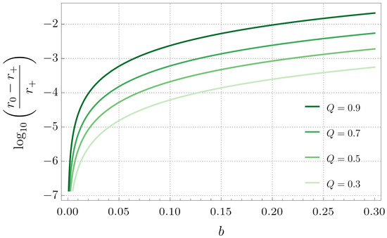
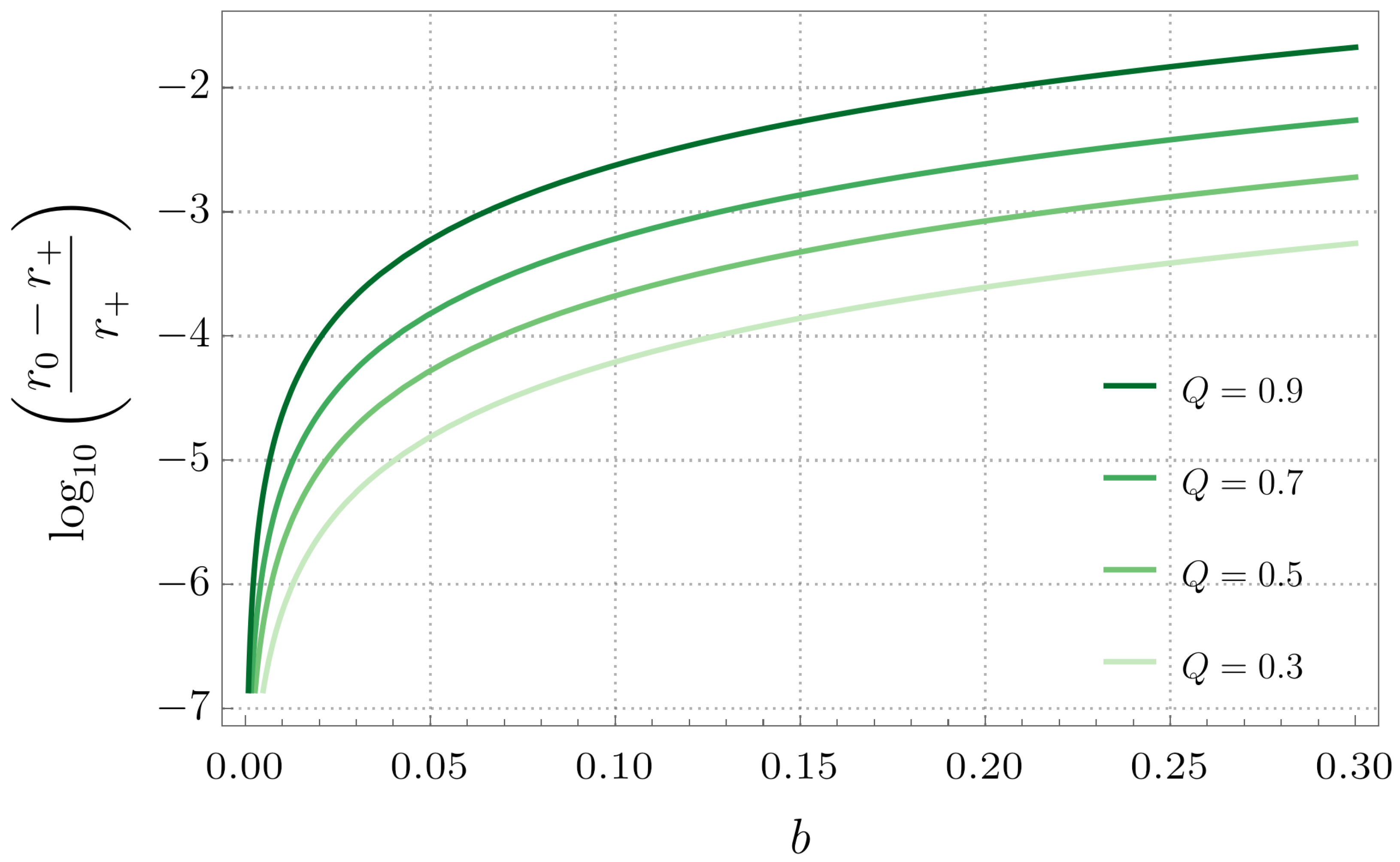
The metric (9), together with (14), describes a static and spherically symmetric wormhole in Bopp–Podolsky electrodynamics [34]. The wormhole throat radius $r_0$ is determined by the vanishing of the inverse radial metric component $g^{rr}$, equivalently $h\left(r_0\right)=0$. Note that the coupling constant b may be interpreted as a parameter controlling deviations from the Reissner–Nordström geometry. In the limit $b=0$, one obtains $f\left(r\right)=h\left(r\right)=\mathrm{\Delta }\left(r\right)$, and the Reissner–Nordström black hole is recovered, with $r_0=r_{+}:=M+\sqrt{M^2-Q^2}$ denoting the event horizon of the spacetime. To quantify the differences between the location of the event horizon of the Reissner–Nordström black hole and the location of the wormhole throat, we plot in Figure 1 the relative difference $(r_0-r_{+})/r_{+}$ as a function of the Podolsky parameter b for several values of the charge Q. We observe that the relative difference increases with both b and Q. In particular, for $b\le 0.01$, the relative difference remains below $0.01\%$ for all values of charge analyzed. For $Q=0.5$ and $b=0.3$, the difference is approximately $0.2\%$.

Figure 1. Relative difference between the wormhole throat radius $r_0$ and the Reissner–Nordström event horizon radius $r_{+}$, for configurations with the same mass M and charge Q, as a function of the Podolsky parameter b. Each curve corresponds to $M=1$ and a different value of the charge Q.

To characterize the wormhole geometry, we introduce the proper radial coordinate $L\left(r\right)$, defined by

$${\displaystyle \frac{dL}{dr}}={\displaystyle \frac{r}{\sqrt{h\left(r\right)}}},$$

(17)

such that $L=0$ at the throat $r=r_0$. The areal radius r has a local minimum with respect to the proper distance at $r=r_0$. Following the seminal work by Morris and Thorne [38], the coordinate $L\left(r\right)$ can be extended to $L<0$, so that the full domain $L\in (-\infty ,\infty )$ connects two asymptotically flat regions through the throat located at $L=0$ [34,39]. Thus, the geometry described by (9) corresponds to a traversable wormhole, allowing the propagation of fields or particles between two causally connected universes.

3. Superradiant Scattering of Scalar Fields

We consider a massless test scalar field $\psi$, with electric charge q, propagating on the wormhole spacetime described by (9). The interaction between the scalar field and the background is governed by the Klein–Gordon equation

$$\begin{array}{cc}\hfill \left({\mathsf{\nabla }}_{\mu }+iq{A}_{\mu }\right)\left({\nabla }^{\mu }+iq{A}^{\mu }\right)\psi & =\hfill \\ \hfill \left[{\displaystyle \frac{1}{\sqrt{-g}}}{\mathsf{\partial }}_{\mu }\left(g^{\mu \nu }\sqrt{-g}{\mathsf{\partial }}_{\nu }\right)+2iq{A}^{\mu }{\mathsf{\partial }}_{\mu }-q^2{A}^{\mu }{A}_{\mu }\right]\psi & =0.\hfill \end{array}$$

(18)

Due to the spherical symmetry and the static nature of the spacetime, the above equation can be separated if we decompose the scalar field into wave modes of frequency $\omega >0$, orbital number $\mathsf{\ell }\in \mathbb{N}$, and azimuthal number $m\in \mathbb{Z}$ satisfying $\mathsf{\ell }\ge \left|m\right|$. More precisely, if we consider the following ansatz,

$$\mathrm{\Phi }(t,r,\theta ,\phi )=R\left(r\right)Y_{\mathsf{\ell }m}(\theta ,\phi )e^{-i\omega t},$$

(19)

where $Y_{\mathsf{\ell }m}$ are the spherical harmonics of the indices ℓ and m, the Klein–Gordon equation reduces to a single ordinary differential equation for the unknown radial function $R\left(r\right)$. After some simplifications, the resulting equation takes the form

$${\displaystyle \frac{d}{dr}}\left(\sqrt{fh}{\displaystyle \frac{dR}{dr}}\right)+\left({\displaystyle \frac{r^4{K}^2}{\sqrt{fh}}}-\mathsf{\ell }(\mathsf{\ell }+1)\sqrt{{\displaystyle \frac{f}{h}}}\right)R=0,$$

(20)

where $K=K\left(r\right)=\omega -q\varphi \left(r\right)$.

To recast the radial Equation (20) into a Schrödinger-like equation, we define $\mathrm{\Psi }\left(r\right)=rR\left(r\right)$ and introduce the tortoise coordinate $r_{*}$ through the relation

$${\displaystyle \frac{d{r}_{*}}{dr}}={\displaystyle \frac{r^2}{\sqrt{f\left(r\right)h\left(r\right)}}}.$$

(21)

In terms of these new variables, Equation (20) transforms into

$${\displaystyle \frac{d^2\mathrm{\Psi }}{d{r}_{*}^2}}+\left[{\left(\omega -q\varphi \left(r\right)\right)}^2-V\left(r\right)\right]\mathrm{\Psi }=0,$$

(22)

where

$$V\left(r\right)=-{\displaystyle \frac{2fh}{r^6}}+{\displaystyle \frac{1}{2r^5}}{\displaystyle \frac{d\left(fh\right)}{dr}}+{\displaystyle \frac{\mathsf{\ell }(\mathsf{\ell }+1)f}{r^4}}$$

(23)

is the effective potential. To make the dependence on the Podolsky parameter b explicit, we use the notation $V=V_b$ and $\varphi ={\varphi }_b$. Given that the spacetime is asymptotically flat, far away from the wormhole (i.e., $r\to \infty$) solutions of the wave Equation (22) are linear combinations of ingoing ($e^{-i\omega r_{*}}$) and outgoing waves ($e^{+i\omega r_{*}}$). On the other hand, near the wormhole’s throat (i.e., $r\to r_0$), solutions of the wave equation are linear combinations of $e^{\pm i\kappa r_{*}}$, where $\kappa$ is the wavenumber defined by

$${\kappa }^2={(\omega -q\varphi \left(r_0\right))}^2-{\displaystyle \frac{f\left(r_0\right)}{r_0^4}}\left[\mathsf{\ell }(\mathsf{\ell }+1)+{\displaystyle \frac{h^{\prime }\left(r_0\right)}{2r_0}}\right].$$

(24)

To ensure oscillatory behavior near the throat, we consider only frequencies satisfying ${\kappa }^2\ge 0$.

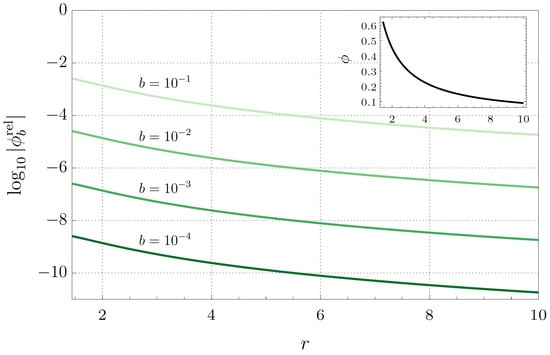
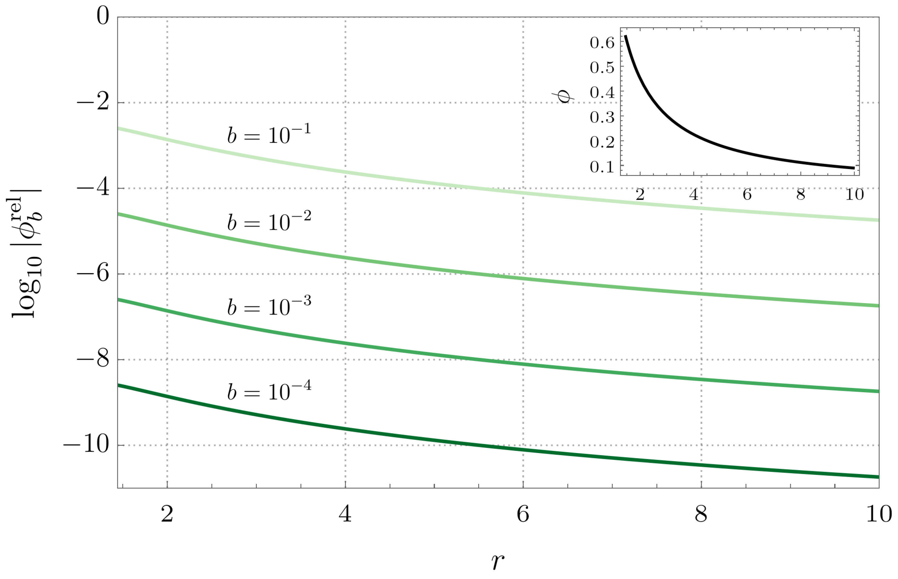
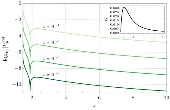
The spacetime geometry is encoded in the electrostatic potential $\varphi \left(r\right)$ and the effective potential $V\left(r\right)$. To illustrate how the parameter b affects the background geometry and, consequently, the scattering process, we plot in Figure 2 the relative difference between the electrostatic potentials for a Bopp–Podolsky wormhole ($b\ne 0$) and a Reissner–Nordström black hole ($b=0$) when $M=1$ and $Q=0.9$. This relative difference is defined as

$${\varphi }_b^{\mathrm{rel}}\left(r\right)={\displaystyle \frac{{\varphi }_b\left(r\right)-{\varphi }_0\left(r\right)}{{\varphi }_0\left(r\right)}}.$$

(25)

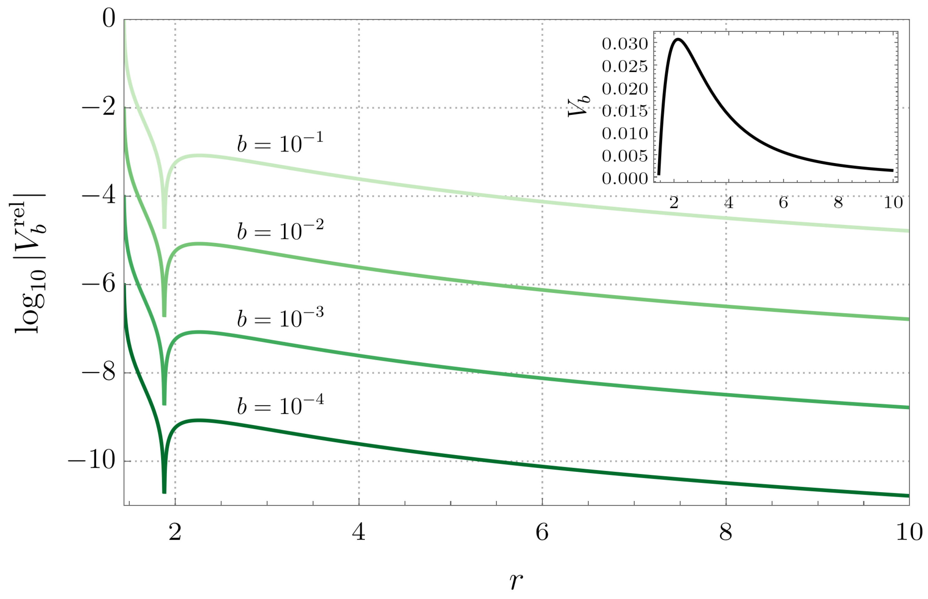
Similarly, in Figure 3 we plot the relative difference between the effective potentials, defined by

$$V_b^{\mathrm{rel}}\left(r\right)={\displaystyle \frac{V_b\left(r\right)-V_0\left(r\right)}{V_0\left(r\right)}},$$

(26)

when $\mathsf{\ell }=0$. In each plot, the inset depicts the Reissner–Nordström potential, which is visually indistinguishable from its Bopp–Podolsky counterpart when $b\ll M$. We note that the electrostatic potential for the wormhole is always weaker than the electrostatic potential of the Reissner–Nordström black hole. In contrast, the effective potential for the wormhole lies above the Reissner–Nordström effective potential at large radii, and below it at small radii. The apparent minima in Figure 3, around $r=2$, correspond to the radii at which the effective potentials coincide, leading to a divergence in the logarithm.

Figure 2. Relative difference ${\varphi }_b^{\mathrm{rel}}$ between the electrostatic potentials for a Bopp–Podolsky wormhole ($b\ne 0$) and a Reissner–Nordström black hole ($b=0$) when $M=1$ and $Q=0.9$ for different values of the parameter b. The inset shows the Reissner–Nordström potential, which is visually indistinguishable from its Bopp–Podolsky counterpart when $b\ll M$. As b increases the curves become progressively lighter and the deviation from the Reissner–Nordström metric grows.

Figure 3. Relative difference $V_b^{\mathrm{rel}}$ between the effective potentials for a Bopp–Podolsky wormhole ($b\ne 0$) and a Reissner–Nordström black hole ($b=0$) when $M=1$, $Q=0.9$, and $\mathsf{\ell }=0$ for different values of the parameter b. The inset shows the Reissner–Nordström potential, which is visually indistinguishable from its Bopp–Podolsky counterpart when $b\ll M$. As b increases the curves become progressively lighter and the deviation from the Reissner–Nordström metric grows.

Another important distinction between the scattering of scalar waves by a Reissner–Nordström black hole and by a Bopp–Podolsky wormhole lies in their different causal structures. In principle, this difference should manifest itself through the boundary conditions imposed on the differential Equation (20). The proper radial coordinate introduced in (17) makes the regular structure of the spacetime explicit, with a bridge connecting two asymptotically flat regions. Following Refs. [19,20,21,22], we adopt a no-return condition for waves crossing the wormhole throat. In this scenario, waves that pass through the throat of the traversable wormhole (located at $L=0$) propagate from the region $L>0$ to the region $L<0$, while no waves traverse the throat in the opposite direction.

Although the physical interpretation differs from the black hole case, where one assumes that no waves propagate from inside the horizon to the exterior, the resulting boundary condition is mathematically analogous in both situations. In both cases, one effectively imposes a one-way propagation condition at the inner boundary of the problem. The solution of (22) that accounts for this boundary condition is

$$\mathrm{\Psi }\left(r_{*}\right)=\left\{\begin{array}{cc}{Y}_t{e}^{-i\kappa r_{*}},\hfill & r_{*}\to -\infty ,\hfill \\ Y_i{r}_{*}^{iqQ}{e}^{-i\omega r_{*}}+Y_r{r}_{*}^{-iqQ}{e}^{i\omega r_{*}},\hfill & r_{*}\to +\infty ,\hfill \end{array}\right.$$

(27)

where $Y_i$, $Y_r$ and $Y_t$ represent, respectively, the amplitudes of the incoming, reflected and transmitted waves.

The scattering amplitudes can be combined into a conservation relation for the energy flux. Taking into account the constancy of the Wronskian between $\mathrm{\Psi }$ and its complex conjugate, we obtain

$$\mathcal{R}+\mathcal{T}=1,$$

(28)

where the reflection coefficient $\mathcal{R}$ and the transmission coefficient $\mathcal{T}$ are defined as

$$\mathcal{R}={\displaystyle \frac{{\left|R\right|}^2}{{\left|I\right|}^2}},\mathcal{T}={\displaystyle \frac{\kappa }{\omega }}{\displaystyle \frac{{\left|T\right|}^2}{{\left|I\right|}^2}}.$$

(29)

The sign of $\kappa$, defined through Equation (24), is chosen such that the group velocity of the wave near the throat, $-\mathsf{\partial }\omega /\mathsf{\partial }\kappa$, is negative. This corresponds to waves propagating from the region $L>0$ toward $L<0$. The phase velocity, $-\omega /\kappa$, however, depends on the sign of $\kappa$ and may therefore be either positive or negative. For sufficiently small $\omega$, one finds that $\kappa$ becomes negative, implying that the phase velocity is directed outward at the wormhole throat. In this regime, the energy flux is opposite to the direction of wave propagation, so that the reflected wave carries more energy than the incident one, thus extracting energy from the wormhole. This amplification characterizes the phenomenon of superradiance.

We remark that the boundary condition considered in this work corresponds to a perfectly absorbing throat. If transmission from the region $L<0$ to the region $L>0$ were allowed, the asymptotic behavior near the throat, described by (27), would also include the outgoing mode $e^{+i\kappa r_{*}}$ in the limit $r_{*}\to -\infty$. In this case, the reflection coefficient $\mathcal{R}$ would receive an additional contribution from flux originating in the $L<0$ region, and any resulting enhancement should therefore be interpreted with care. Such an enhancement would not necessarily correspond to the standard notion of superradiant amplification, as it could originate from flux transmitted through the throat from the $L<0$ region rather than from energy extraction driven by waves incident from $L>0$.

In terms of the scattering coefficients, superradiance manifests itself through a reflection coefficient larger than unity and a negative transmission coefficient. It is customary to quantify this amplification through the factor Z, defined as the relative increase in the reflected flux with respect to the incident one [8],

$$Z\equiv \mathcal{R}-1=-\mathcal{T}.$$

(30)

The parameter Z, therefore, measures the fraction of energy gained or lost during the scattering process. When $Z>0$, the reflected wave is amplified and superradiance occurs, whereas $Z<0$ corresponds to attenuation of the wave, indicating absorption of energy by the wormhole. As before, to make the dependence on the Podolsky parameter b explicit, we use the notation $Z=Z_b\left(\omega \right)$.

4. Amplification Factors

We solve Equation (20) numerically, using Equation (27) to implement the initial conditions and extract the reflection and transmission coefficients. In particular, to investigate the influence of the Podolsky parameter b on superradiance, we compute the amplification factor Z for several choices of parameters and compare the results with those obtained in the standard Reissner–Nordström black hole scenario.

The numerical scheme consists of solving the initial value problem defined by Equation (20) together with the initial conditions

$$\begin{array}{cc}\hfill R\left(r_i\right)& =\sqrt{r_0ϵ},\hfill \end{array}$$

(31a)

$$\begin{array}{cc}\hfill R^{\prime }\left(r_i\right)& ={\displaystyle \frac{-i\kappa r_0^2}{\sqrt{f\left(r_0\right)h^{\prime }\left(r_0\right)}}},\hfill \end{array}$$

(31b)

with the initial point chosen as $r_i=r_0(1+ϵ)$, where $ϵ\ll 1$ parameterizes the distance from the wormhole’s throat. Note that the above initial conditions correspond to Equation (27) with $Y_t=1$. Because the differential equation is linear, the solution for an arbitrary value of $Y_t$ can then be obtained by a simple rescaling.

We integrate the initial value problem up to $r_f$, where the values of $R\left(r_f\right)$ and $R^{\prime }\left(r_f\right)$ are extracted. These are then substituted into Equation (27) to determine the coefficients $Y_i$ and $Y_r$. Numerical accuracy is improved by including subleading terms in the asymptotic expansion (27) up to order $r^{-4}$. Convergence of the results is verified by varying the parameters $ϵ$ and $r_f$. We typically use $ϵ={10}^{-8}$ and $r_f={10}^4{r}_0$, which are generally sufficient to ensure numerical convergence, although more stringent choices may be required for very small $\omega$ or near-extremal charges.

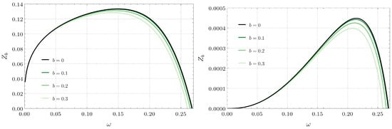
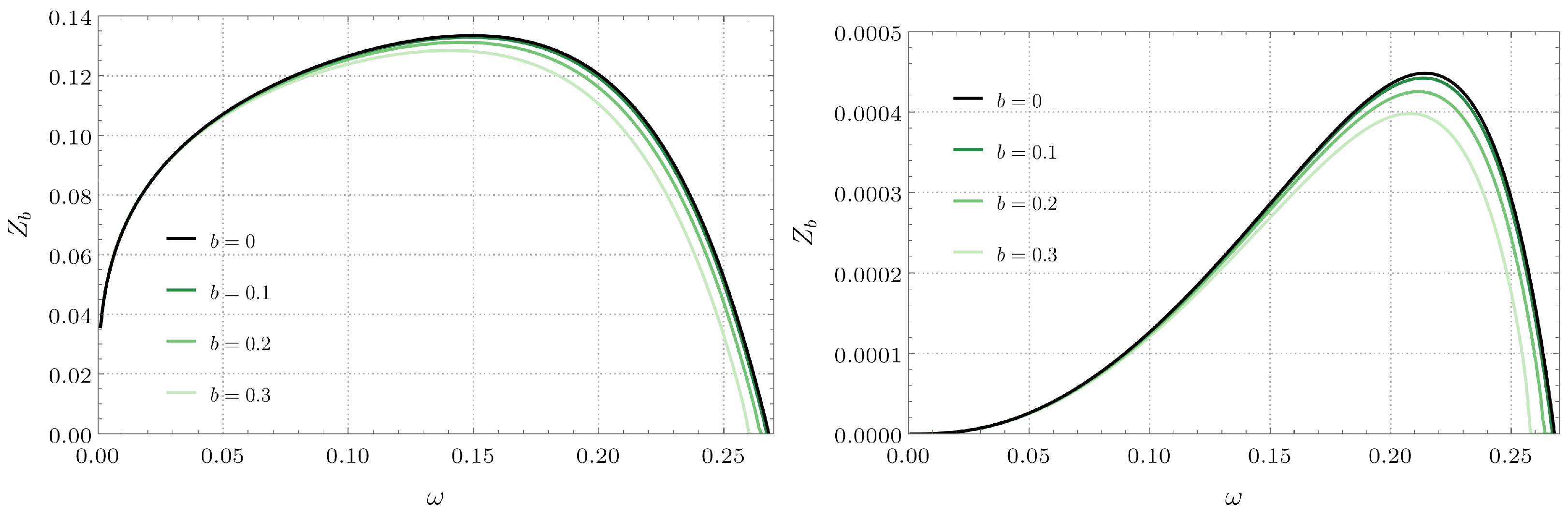
In Figure 4, we present the amplification factor for the Bopp–Podolsky wormhole with $M=1$ and $Q=0.5$, highlighting the effect of the parameter b for $\mathsf{\ell }=0$ (left panel) and $\mathsf{\ell }=1$ (right panel) when $q=1$. The results show that superradiance occurs in Bopp–Podolsky electrodynamics and demonstrate that the coupling parameter b tends to suppress the amplification in comparison to the Reissner–Nordström case. In particular, as b increases, the amplification factor $Z_b$ decreases for a given frequency $\omega$. Another notable feature is that the range of superradiant frequencies shrinks as b increases. This behavior indicates that deviations from the Reissner–Nordström solution, parameterized by the coupling constant b, effectively inhibit energy extraction due to superradiance.

Figure 4. Superradiant amplification factor $Z=Z_b\left(\omega \right)$ for $\mathsf{\ell }=0$ (left panel) and $\mathsf{\ell }=1$ (right panel) charged scalar perturbations ($q=1$) around Bopp–Podolsky wormholes with mass $M=1$ and charge $Q=0.5$ for different values of the parameter b. The black solid line represents the Reissner–Nordström black hole ($b=0$), and the curves become progressively lighter as b increases.

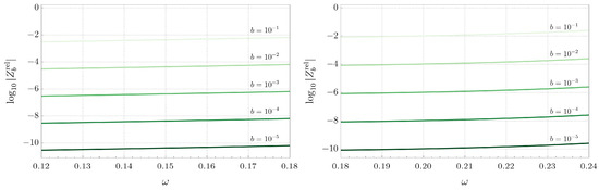
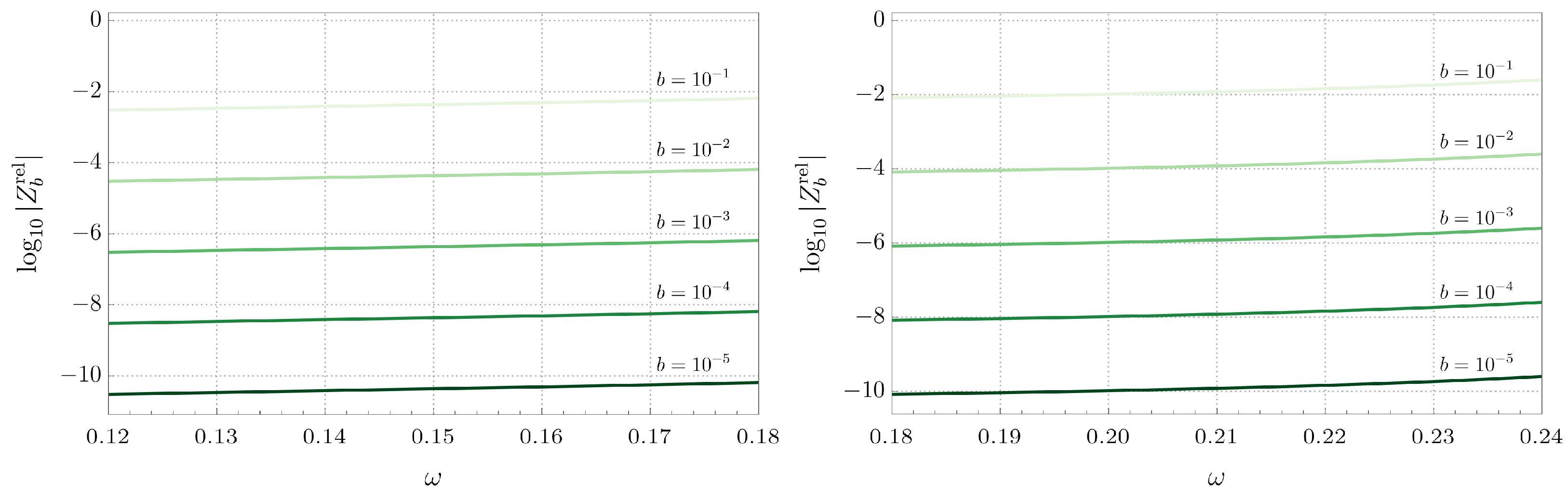
To further explore the quantitative differences in superradiant scattering between Bopp–Podolsky wormholes and Reissner–Nordström black holes, we focus on the regime $b\sim \mathcal{O}\left({10}^{-5}\right)$–$\mathcal{O}\left({10}^{-2}\right)$. We consider frequencies near the peak of superradiant amplification shown in Figure 4, which occurs around $\omega \approx 0.15$ for $\mathsf{\ell }=0$ (left panel) and $\omega \approx 0.22$ for $\mathsf{\ell }=1$ (right panel). In this regime, we compute the relative difference between the corresponding amplification factors for Bopp–Podolsky wormholes and Reissner–Nordström black holes, defined as

$$Z_b^{\mathrm{rel}}\left(\omega \right)={\displaystyle \frac{Z_b\left(\omega \right)-Z_0\left(\omega \right)}{Z_0\left(\omega \right)}}.$$

(32)

The results are shown in Figure 5. We observe that the suppression of superradiant amplification for Bopp–Podolsky wormholes is small, typically of order $b^2/M^2$, consistent with the perturbative regime underlying the wormhole solution. Consequently, in the regime $b\ll M$ the phenomenology of superradiant scattering remains largely indistinguishable from the Reissner–Nordström case, suggesting that differences between Maxwell and Bopp–Podolsky electrodynamics would be challenging to detect through superradiance alone.

Figure 5. Relative difference of the superradiant amplification factor between Bopp–Podolsky wormholes and Reissner–Nordström black holes when $M=1$, $Q=0.5$, and $q=1$. The (left panel) corresponds to $\mathsf{\ell }=0$ and depicts the frequency range $[0.12,0.18]$ around the peak of the black curve shown in the left panel of Figure 4. The (right panel) corresponds to $\mathsf{\ell }=1$ and depicts the frequency range $[0.18,0.24]$ around the peak of the black curve shown in the right panel of Figure 4. As b increases the curves become progressively lighter and the deviation from the Reissner–Nordström metric grows.

The suppression of superradiance can be qualitatively understood through the analysis of the effective potential and the electrostatic potential. As the Podolsky parameter b increases from zero, the peak of the potential barrier increases (see Figure 3), making it increasingly difficult for waves to cross the potential barrier. Consequently, a smaller fraction of the incident energy flux reaches the throat. Similarly, the energy flux propagating from the wormhole towards infinity is also reduced, thus contributing to the suppression of superradiance. The effect of the electrostatic potential follows from Equations (24) and (29). As shown in Figure 2, increasing b weakens the electrostatic potential. Therefore, the wavenumber $\kappa$, defined through Equation (24), becomes less negative and, hence, the transmission coefficient $\mathcal{T}$, defined in Equation (29), also becomes less negative, leading to a suppression of the superradiant reflection coefficient $\mathcal{R}$.

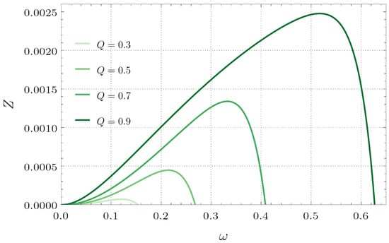
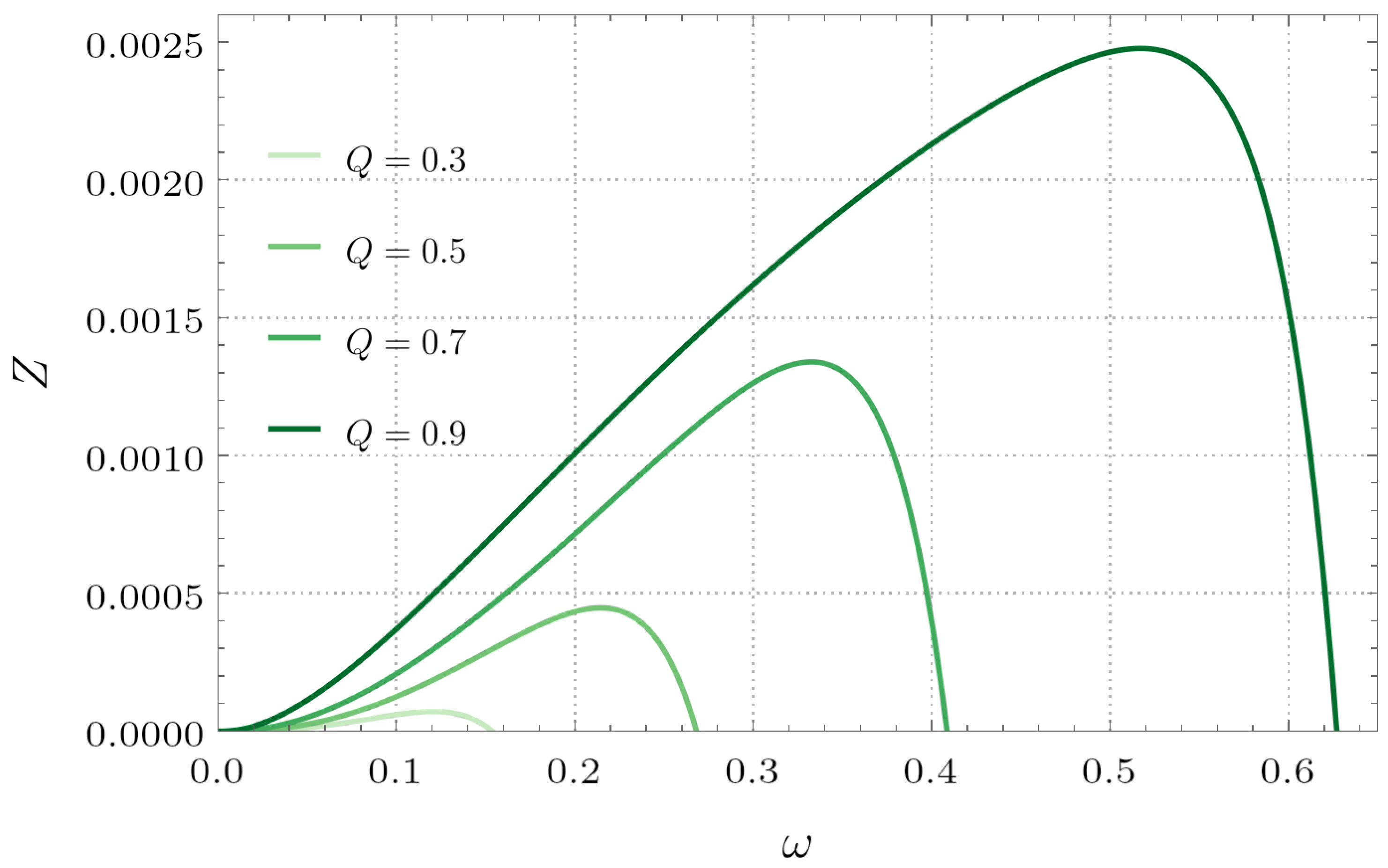
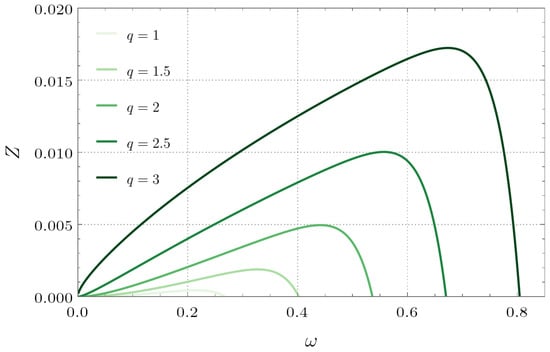
Finally, in Figure 6, we fix the coupling parameter $b=0.01$, the orbital number $\mathsf{\ell }=1$, the field charge $q=1$, and present the amplification factors for the Bopp–Podolsky wormhole with $M=1$ as the wormhole charge varies from $Q=0.3$ to $Q=0.9$. Similarly, in Figure 7, we fix $b=0.01$, $\mathsf{\ell }=1$, $Q=0.5$, and $M=1$, and present the amplification factor as the field charge varies from $q=1$ to $q=3$. We observe that increasing either the wormhole charge Q or the field charge q enhances superradiant amplification, both in magnitude and across a wider frequency range. This behavior reflects the strengthening of the electromagnetic coupling $qQ$ and exhibits no qualitative differences from superradiance in Reissner–Nordström black holes.

Figure 6. Superradiant amplification factor $Z=Z_b\left(\omega \right)$ for $\mathsf{\ell }=1$ charged scalar perturbations ($q=1$) around Bopp–Podolsky wormholes with mass $M=1$ and Podolsky parameter $b=0.01$ for different values of the charge Q. The curves become progressively darker as Q increases.

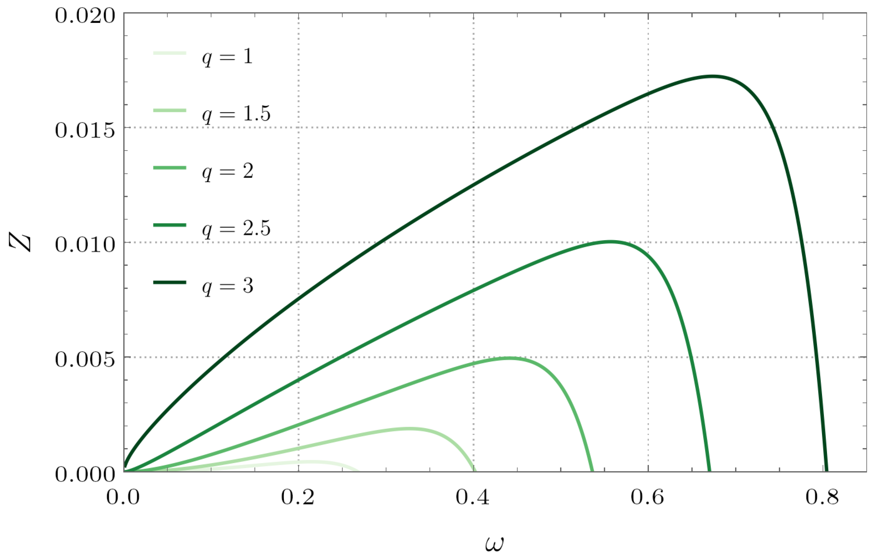
Figure 7. Superradiant amplification factor $Z=Z_b\left(\omega \right)$ for $\mathsf{\ell }=1$ charged scalar perturbations around Bopp–Podolsky wormholes with mass $M=1$, charge $Q=0.5$ and Bopp–Podolsky parameter $b=0.01$ for different values of the scalar charge q. The curves become progressively darker as q increases.

5. Conclusions

In this work, we have analyzed the superradiant scattering of scalar waves in the background of Bopp–Podolsky wormholes, focusing on how deviations from Maxwell electrodynamics, parameterized by the coupling constant b, affect the amplification factor. The underlying geometry provides a natural setting to explore wormhole configurations within a modified electrodynamics framework. From the scalar wave equation, we derived the relevant effective potential and implemented a numerical scheme to compute the reflection and transmission coefficients, and hence the superradiant amplification factor. We have adopted boundary conditions that allow waves to cross the throat in one direction only, with no incoming flux from the opposite asymptotic region.

Our results show that the parameter b tends to suppress superradiant amplification. As b increases, both the magnitude of the amplification factor and the range of superradiant frequencies decrease, indicating that deviations from Maxwell electrodynamics inhibit the efficiency of energy extraction. This behavior is robust across different multipoles and parameter choices. From a comparative perspective, the deviations we find with respect to the Reissner–Nordström case are systematic but quantitatively small in the regime $b\ll M$. In particular, the suppression of the amplification factor and the narrowing of the superradiant frequency window provide clear signatures of Bopp–Podolsky electrodynamics at the theoretical level. However, the magnitude of these effects decreases rapidly as $b\to 0$, making them increasingly difficult to resolve.

We remark that, for Reissner–Nordström black holes, superradiant scattering relies on the dissipative nature of the event horizon, which absorbs negative-energy modes and prevents their return to the exterior region. The boundary condition employed in this work plays a similar role: it effectively imposes perfect absorption at the wormhole throat, so that negative-energy modes traversing the throat from $L>0$ to $L<0$ never return, thus enabling superradiant scattering. If, however, wave propagation from $L<0$ to $L>0$ is allowed, the repeated reflection and amplification of negative-energy modes may trigger instabilities commonly associated with horizonless compact objects, such as wormholes and gravastars [21,40].

It is important to emphasize that electrically charged black holes are not expected to be realized in realistic astrophysical environments. Any net electric charge is efficiently neutralized by opposite charges [41]. Even tiny charge imbalances generate electric fields strong enough to attract ambient charges and rapidly discharge the object, leading to effectively neutral configurations on very short timescales. As a result, Reissner–Nordström black holes, and their generalizations, are best viewed as theoretical laboratories rather than direct astrophysical models. In this light, the present results should be interpreted as a controlled framework to assess how modifications induced by Bopp–Podolsky electrodynamics affect superradiant amplification.

A more promising route toward experimental relevance is provided by purely electrodynamical realizations of superradiance based on Zel’dovich’s cylinder [1,2,3,4]. Recent experiments [42,43] reported the observation of superradiant amplification and related instabilities in electromagnetic circuits, providing a concrete realization of Zel’dovich’s superradiance. From this perspective, a natural extension of the present work would be to analyze superradiant amplification in purely electromagnetic setups governed by generalized electrodynamics, such as the Bopp–Podolsky theory. This would allow one to directly assess how alternatives to Maxwell electrodynamics modify the amplification factor in experimentally accessible configurations, potentially leading to observable signatures.

Finally, it is worth noting that superradiance is closely connected to other energy extraction mechanisms involving electromagnetic fields in strong gravity. A prominent example is the Blandford–Znajek process [44], which describes the extraction of rotational energy from a Kerr black hole via magnetized plasma. Although the present analysis is restricted to static, charged configurations, it would be interesting to explore how Bopp–Podolsky-type corrections would affect such mechanisms.

References

- Zel’Dovich, Y.B. Generation of Waves by a Rotating Body. JETP Lett. 1971, 14, 180. [Google Scholar]
- Zel’Dovich, Y.B. Amplification of Cylindrical Electromagnetic Waves Reflected from a Rotating Body. Sov. Phys. JETP 1972, 35, 1085. [Google Scholar]
- Zel’dovich, Y.B.; Rozhanskii, L.V.; Starobinskii, A.A. Rotating bodies and electrodynamics in a rotating coordinate system. Radiophys. Quantum Electron. 1986, 29, 761–768. [Google Scholar] [CrossRef] [Scilit]
- Bekenstein, J.D.; Schiffer, M. The Many faces of superradiance. Phys. Rev. D 1998, 58, 064014. [Google Scholar] [CrossRef] [Scilit]
- Misner, C. Stability of Kerr black holes against scalar perturbations. Bull. Am. Phys. Soc. 1972, 17, 472. [Google Scholar]
- Starobinsky, A.A. Amplification of waves reflected from a rotating “black hole”. Sov. Phys. JETP 1973, 37, 28–32. [Google Scholar]
- Starobinsky, A.A.; Churilov, S.M. Amplification of electromagnetic and gravitational waves scattered by a rotating “black hole”. Sov. Phys. JETP 1974, 38, 1. [Google Scholar]
- Brito, R.; Cardoso, V.; Pani, P. Superradiance: New Frontiers in Black Hole Physics; Lecture Notes in Physics; Springer: Cham, Switzerland, 2020; Volume 971, pp. 1–293. [Google Scholar] [CrossRef] [Scilit]
- Richartz, M.; Weinfurtner, S.; Penner, A.J.; Unruh, W.G. Generalized superradiant scattering. Phys. Rev. D 2009, 80, 124016. [Google Scholar] [CrossRef] [Scilit]
- Penrose, R. “Golden Oldie”: Gravitational collapse: The role of general relativity. Gen. Relativ. Gravit. 2002, 34, 1141–1165. [Google Scholar] [CrossRef] [Scilit]
- Penrose, R.; Floyd, R.M. Extraction of rotational energy from a black hole. Nature 1971, 229, 177–179. [Google Scholar] [CrossRef] [Scilit]
- Bekenstein, J.D. Extraction of energy and charge from a black hole. Phys. Rev. D 1973, 7, 949–953. [Google Scholar] [CrossRef] [Scilit]
- Benone, C.L.; Crispino, L.C.B. Superradiance in static black hole spacetimes. Phys. Rev. D 2016, 93, 024028. [Google Scholar] [CrossRef] [Scilit]
- Christodoulou, D.; Ruffini, R. Reversible transformations of a charged black hole. Phys. Rev. D 1971, 4, 3552–3555. [Google Scholar] [CrossRef] [Scilit]
- Richartz, M.; Saa, A. Superradiance without event horizons in General Relativity. Phys. Rev. D 2013, 88, 044008. [Google Scholar] [CrossRef] [Scilit]
- Cardoso, V.; Brito, R.; Rosa, J.L. Superradiance in stars. Phys. Rev. D 2015, 91, 124026. [Google Scholar] [CrossRef] [Scilit]
- Day, F.V.; McDonald, J.I. Axion superradiance in rotating neutron stars. J. Cosmol. Astropart. Phys. 2019, 10, 051. [Google Scholar] [CrossRef] [Scilit]
- Cardoso, V.; Pani, P.; Yu, T.T. Superradiance in rotating stars and pulsar-timing constraints on dark photons. Phys. Rev. D 2017, 95, 124056. [Google Scholar] [CrossRef] [Scilit]
- Lima, H.C.D.; Benone, C.L.; Crispino, L.C.B. Scalar absorption: Black holes versus wormholes. Phys. Rev. D 2020, 101, 124009. [Google Scholar] [CrossRef]
- Lima Junior, H.C.D.; Benone, C.L.; Crispino, L.C.B. Scalar scattering by black holes and wormholes. Eur. Phys. J. C 2022, 82, 638. [Google Scholar] [CrossRef] [Scilit]
- Franzin, E.; Liberati, S.; Mazza, J.; Dey, R.; Chakraborty, S. Scalar perturbations around rotating regular black holes and wormholes: Quasinormal modes, ergoregion instability, and superradiance. Phys. Rev. D 2022, 105, 124051. [Google Scholar] [CrossRef] [Scilit]
- Bao, S.S.; Hou, S.; Zhang, H. Searching for wormholes with gravitational wave scattering. Eur. Phys. J. C 2023, 83, 127. [Google Scholar] [CrossRef] [Scilit]
- Podolsky, B. A Generalized Electrodynamics Part I-Non-Quantum. Phys. Rev. 1942, 62, 68–71. [Google Scholar] [CrossRef] [Scilit]
- Podolsky, B.; Kikuchi, C. A Generalized Electrodynamics Part II-Quantum. Phys. Rev. 1944, 65, 228–235. [Google Scholar] [CrossRef] [Scilit]
- Podolsky, B.; Schwed, P. Review of a Generalized Electrodynamics. Rev. Mod. Phys. 1948, 20, 40. [Google Scholar] [CrossRef] [Scilit]
- Galvao, C.A.P.; Pimentel Escobar, B.M. The Canonical Structure of Podolsky Generalized Electrodynamics. Can. J. Phys. 1988, 66, 460–466. [Google Scholar] [CrossRef] [Scilit]
- Cuzinatto, R.R.; de Melo, C.A.M.; Pompeia, P.J. Second order gauge theory. Ann. Phys. 2007, 322, 1211–1232. [Google Scholar] [CrossRef] [Scilit]
- Bertin, M.C.; Pimentel, B.M.; Zambrano, G.E.R. The Canonical structure of Podolsky’s generalized electrodynamics on the Null-Plane. J. Math. Phys. 2011, 52, 102902. [Google Scholar] [CrossRef] [Scilit]
- Mascaro, B.; Siciliano, G. Positive Solutions For a Schrödinger-Bopp-Podolsky system in R3. arXiv 2020, arXiv:2009.08531. [Google Scholar] [CrossRef] [Scilit]
- Siciliano, G. Normalized solutions for Schrödinger-Bopp-Podolsky systems in bounded domains. arXiv 2025, arXiv:2504.10385. [Google Scholar] [CrossRef] [Scilit]
- Lazar, M.; Leck, J. Second Gradient Electromagnetostatics: Electric Point Charge, Electrostatic and Magnetostatic Dipoles. Symmetry 2020, 12, 1104. [Google Scholar] [CrossRef] [Scilit]
- Borges, L.H.C.; Barone, F.A.; de Melo, C.A.M.; Barone, F.E. Higher order derivative operators as quantum corrections. Nucl. Phys. B 2019, 944, 114634. [Google Scholar] [CrossRef] [Scilit]
- Cuzinatto, R.R.; de Melo, C.A.M.; Medeiros, L.G.; Pimentel, B.M.; Pompeia, P.J. Bopp–Podolsky black holes and the no-hair theorem. Eur. Phys. J. C 2018, 78, 43. [Google Scholar] [CrossRef] [Scilit]
- Frizo, D.A.; de Melo, C.A.M.; Medeiros, L.G.; Neves, J.C.S. Viable wormhole solution in Bopp–Podolsky electrodynamics. Ann. Phys. 2023, 457, 169411. [Google Scholar] [CrossRef] [Scilit]
- Bekenstein, J.D. Nonexistence of baryon number for static black holes. Phys. Rev. D 1972, 5, 1239–1246. [Google Scholar] [CrossRef] [Scilit]
- Bekenstein, J.D. Nonexistence of baryon number for black holes. ii. Phys. Rev. D 1972, 5, 2403–2412. [Google Scholar] [CrossRef] [Scilit]
- Mayo, A.E.; Bekenstein, J.D. No hair for spherical black holes: Charged and nonminimally coupled scalar field with selfinteraction. Phys. Rev. D 1996, 54, 5059–5069. [Google Scholar] [CrossRef] [Scilit]
- Morris, M.S.; Thorne, K.S. Wormholes in space-time and their use for interstellar travel: A tool for teaching general relativity. Am. J. Phys. 1988, 56, 395–412. [Google Scholar] [CrossRef] [Scilit]
- Raza, M.A.; Tello-Ortiz, F.; Zubair, M.; Gómez-Leyton, Y. Some optical properties of rotating wormhole in Bopp-Podolsky electrodynamics. J. Cosmol. Astropart. Phys. 2025, 2025, 065. [Google Scholar] [CrossRef] [Scilit]
- Cardoso, V.; Pani, P.; Cadoni, M.; Cavaglia, M. Instability of hyper-compact Kerr-like objects. Class. Quant. Grav. 2008, 25, 195010. [Google Scholar] [CrossRef] [Scilit]
- Gibbons, G.W. Vacuum Polarization and the Spontaneous Loss of Charge by Black Holes. Commun. Math. Phys. 1975, 44, 245–264. [Google Scholar] [CrossRef] [Scilit]
- Braidotti, M.C.; Vinante, A.; Cromb, M.; Sandakumar, A.; Faccio, D.; Ulbricht, H. Amplification of electromagnetic fields by a rotating body. Nat. Commun. 2024, 15, 5453. [Google Scholar] [CrossRef] [Scilit] [PubMed]
- Cromb, M.; Braidotti, M.C.; Vinante, A.; Faccio, D.; Ulbricht, H. Creation of a black hole bomb instability in an electromagnetic system. Sci. Adv. 2025, 11, adz4595. [Google Scholar] [CrossRef] [Scilit]
- Blandford, R.D.; Znajek, R.L. Electromagnetic extractions of energy from Kerr black holes. Mon. Not. Roy. Astron. Soc. 1977, 179, 433–456. [Google Scholar] [CrossRef] [Scilit]
Disclaimer/Publisher’s Note: The statements, opinions and data contained in all publications are solely those of the individual author(s) and contributor(s) and not of MDPI and/or the editor(s). MDPI and/or the editor(s) disclaim responsibility for any injury to people or property resulting from any ideas, methods, instructions or products referred to in the content. |
© 2026 by the authors. Licensee MDPI, Basel, Switzerland. This article is an open access article distributed under the terms and conditions of the Creative Commons Attribution (CC BY) license.