Relativistic Positioning Systems in Flat Space-Time with Inertial, Hyperbolic and Rotating Emitters

Abstract

We analyse different configurations of four emitters in a Relativistic Positioning System (RPS) with: (i) one inertial and three static emitters, (ii) one hyperbolic and three static emitters, and (iii) three rotating and one static emitter. For every configuration, we analyse the emission/reception conditions, represent the emission configuration regions and write the user’s location solution. We follow the notions and terminology of previous works on this topic.

1. Introduction

A Relativistic Positioning System (RPS) is essentially a set of four clocks broadcasting their time by means of electromagnetic signals. Although the time of every clock may be any one, for simplicity, we suppose they broadcast their proper times. The set of four such times imprinted on the signals converging at every space-time event constitutes a (four-dimensional) physical coordinate system for the region reached by the signals. Such coordinates are called emission coordinates [1]. Analogous Newtonian emission coordinate systems were constructed from sonic signals and classified in [2].

In this work, we are mainly concerned with specific RPSs in Minkowski space-time. The affine geometry and light-cone structure of flat space-time make viable analytical constructions of RPSs with both inertial and non-inertial emitters. At first glance, these constructions may seem somewhat academic for practical purposes. However, concrete RPS examples contribute to the development of current RPS theory and future applications. Furthermore, the study of Minkowskian RPSs paves the way for realistic constructions in a known gravitational field, modelled as a curved Lorentzian geometry in which the use of the Ruse–Synge world function for the null geodesics [3,4] or the application of distance geometry concepts [5,6] may be mandatory.

The main aim of RPS theory is to give a precise physical frame for the location of events in a gravitationally unknown region in order to dorelativistic gravimetry, as explained in [6,7,8]. The starting ideas of the theory of RPSs are that in such an unknown region, the first object to be constructed is a physical coordinate system, allowing for identification of its events with the points of the mathematical models in use; that such a physical coordinate system has to be constructed generically by means of electromagnetic signals and with a protocol independent of the particular space-time; and that the over-determined interlacement of these signals contains important information (chronometry in arbitrary directions) on the relativistic gravitational field in which we are immersed.

In [9], we analysed the most elemental example of an RPS construction: four static emitters in flat space-time. In the present work, this construction is extended to RPSs including inertial, accelerated and rotating emitters. These constructions present significant novelties and differences with respect to the static situation and may provide insights on fictitious gravitational potentials attached to non-inertial effects.

The location problem in Minkowski space-time was dealt with in [9,10,11,12]. Developments on the subject are found in [13,14,15,16,17], including numerical treatment and prospects. Refs. [18,19,20] offer relevant notions to develop RPS theory, presenting examples in two-dimensional Lorentzian spaces. General concepts and results in 3D and 4D were communicated in [21].

In this work, we develop RPS examples in Minkowski space-time with four emitters following different motions. In all considered cases, we carry out the same procedure. The satellite trajectories in space-time are written, the emission/reception conditions are stated, the satellite trajectories on the grid of emission coordinates are determined and the RPS solution is interpreted by representing the characteristic regions and working out a simplified positioning example. We used Mathematica software 13.3 to represent the characteristic regions of the RPS solutions and perform numerical calculations.

This article is organized as follows: The terminology of an RPS is introduced in Section 2. Section 3 starts with a positioning example involving one inertial and three static emitters, Section 4 considers an RPS with one hyperbolic and three static emitters, and Section 5 analyses the example of one static and three uniformly rotating emitters. A brief summary and conclusions are presented in Section 6. Appendix A summarizes the notation used herein.

2. RPS Terminology and Summary of Results in Flat Space-Time

Following [10,11], here, we present a compendium of the essential RPS terminology and results used to develop this work in Minkowski space-time.

Relativistic positioning system: A set of four emitters ($A=1, 2, 3, 4$) of world lines (${\gamma }_A\left({\tau }^A\right)$) broadcasting their respective proper times (${\tau }^A$) by means of electromagnetic signals.

Emission coordinates of an event: The four times $\left\{{\tau }^A\right\}$ that are received at each space-time event (x) reached by the emitted signals.

Grid of an RPS: The four-space $\mathcal{T}\equiv \left[{\tau }^1\right]\left[{\tau }^2\right]\left[{\tau }^3\right]\left[{\tau }^4\right]\approx {\mathbb{R}}^4$.

Configuration of the emitters for an event (x): A set of four events ($\left\{{\gamma }_A\left({\tau }^A\right)\right\}$) of the emitters at the emission times ($\left\{{\tau }^A\right\}$) received at x.

In Minkowski space-time, ${\gamma }_A\equiv O{\gamma }_A\left({\tau }^A\right)$ denotes the position four-vectorof emitter A with respect to the origin (O) of an inertial coordinate system ($\left\{x^{\alpha }\right\},A=1, 2, 3, 4$).

Configuration vector (χ): A vector informing the emitter configuration at the emission times $\left\{{\tau }^A\right\}$ received at x, i.e.,

$$\chi =\ast (e_1\wedge e_2\wedge e_3),$$

(1)

with $e_a={\gamma }_a-{\gamma }_4$ ($a=1, 2, 3$) representing the relative positions of emitters 1, 2 and 3 with respect to emitter 4 and where * stands for the Hodge dual operator and ∧ is the exterior product (see Appendix A for index-notation transcriptions). An emitter configuration is regular iff $\chi \ne 0$.

Null propagation equations: Consider the following system of non-linear equations:

$${(x-{\gamma }_A)}^2=0,A=1, 2, 3, 4,$$

(2)

with x representing the user position four-vectorwith respect to O. The solution to these equations is the coordinate transformation from emission to inertial coordinates ($x^{\alpha }\left({\tau }^A\right)$).

Shadow of emitter A to emitter B: Space-time events (x) for which future-directed null vectors $m_A=x-{\gamma }_A$ and $m_B=x-{\gamma }_B$ become collinear, i.e., $m_A·m_B=0$, lying on the future light cone with its vertex at the intersection of $m_A$ (or $m_B$) with ${\gamma }_A$.

For four emitters, there are 12 shadows in total, defining the 12 faces of the shadow dodecahedron $\mathcal{D}$ in the grid of emission coordinates.

Emission/reception conditions: Conditions expressing that the null vectors ($m_A=x-{\gamma }_A$, $A=1, 2, 3, 4$) are all either future- or past-oriented, i.e., $m_A·m_B<0$, $A\ne B$:

$${\left(e_a\right)}^2>0,{(e_a-e_b)}^2>0,a, b=1, 2, 3.$$

(3)

Emission region: The set $\mathcal{R}$ of events reached by the four signals broadcast by the positioning system. Every $x\in \mathcal{R}$ is labelled with the corresponding emission coordinates ($\left\{{\tau }^A\right\}$).

Characteristic emission function: A map ($\mathrm{\Theta }$) that, to every $x\in \mathcal{R}$, associates its emission coordinates, that is, $\mathrm{\Theta }\left(x\right)=\left({\tau }^A\right)$.

Emission coordinate region: A subset ($\mathcal{C}$) of the emission region $\mathcal{R}$ where the gradients ($d{\tau }^A$) are well defined and linearly independent.

Orientation of a relativistic positioning system at the event x: The orientation of its emission coordinates at x or, equivalently, the orientation of the tetrad of 1-forms ($\{d{\tau }^1,d{\tau }^2,d{\tau }^3,d{\tau }^4\}$), given by the sign $\widehat{ϵ}$ of the Jacobian determinant ($j_{\mathrm{\Theta }}\left(x\right)$) of $\mathrm{\Theta }$ at x, $\widehat{ϵ}\equiv \mathit{sgn}{j}_{\mathrm{\Theta }}\left(x\right)$. In terms of the gradients of the emission coordinates, one has

$$\widehat{ϵ}=\mathit{sgn}[*(d{\tau }^1\wedge d{\tau }^2\wedge d{\tau }^3\wedge d{\tau }^4)].$$

(4)

The orientation ($\widehat{ϵ}$) of an RPS at an event (x) is, by definition, the orientation of its emission coordinates at x.

For regular configurations, the region where the vector ($\chi$) is timelike or null, ${\chi }^2\le 0$, is called the central region of the RPS. In it, the orientation is uniform and is given by $\widehat{ϵ}=\mathrm{sgn}(u·\chi )$ for any observer (u). But out of this region, it is not possible to determine $\widehat{ϵ}$ solely based on the world lines (${\gamma }_A\left({\tau }^A\right)$) [10]; additional information is necessary [11].

Solution to the null propagation equations: The solution to (2) or, equivalently, the coordinate transformation from emission to inertial coordinates, is [10]

$$\begin{array}{c}\hfill x={\gamma }_4+y_{*}+\lambda \chi ,\end{array}$$

(5)

with $y_{*}$ representing the particular solution, which is found by bringing in a subsidiary vector ($\xi$) satisfying the transversality condition ($\xi ·\chi \ne 0$):

$$y_{*}={\displaystyle \frac{1}{\xi ·\chi }}i\left(\xi \right)H,$$

(6)

where H is the configuration bivector, i.e.,

$$H={\mathrm{\Omega }}_1{E}^1+{\mathrm{\Omega }}_2{E}^2+{\mathrm{\Omega }}_3{E}^3,$$

(7)

with

$$\begin{array}{c}\hfill E^1=\ast (e_2\wedge e_3),E^2=\ast (e_3\wedge e_1),E^3=\ast (e_1\wedge e_2),\end{array}$$

(8)

and

$$\begin{array}{c}\hfill \lambda =-{\displaystyle \frac{y_{*}^2}{(y_{*}·\chi )+\widehat{ϵ}\sqrt{\mathrm{\Delta }}}},\mathrm{\Delta }={(y_{*}·\chi )}^2-y_{*}^2{\chi }^2.\end{array}$$

(9)

Imposing all six emission/reception conditions (3) is equivalent to requiring that all four $\tau$-coordinates of an event have the same emission or reception character, that is, that all four coordinates are either emission coordinates (the user receives four signals from the satellites that codify the proper times at which they were respectively emitted—generically known as a positioning system) or reception coordinates (the user emits a signal that is received by the satellites at the proper times—generically known as a localization system). Reception coordinates were studied in [22,23]. When studying positioning systems, we want all coordinates to be of the same type—specifically, emission coordinates. Formally, the shadow dodecahedron of a positioning system is the same as that of a localization system for a given satellite configuration. We use the term location system for both positioning and localization systems.

On the other hand, the volume enclosed by the surface of the vanishing Jacobian determinant in the $\tau$ grid contains all events for which there is a solution to the null propagation equations (2). The exterior of this surface has no physical meaning. In RPS theory, where we require that all four coordinates be emission coordinates, the surface of the vanishing Jacobian determinant lies within the shadow dodecahedron. This surface has a number of singular points [9], two of which are also vertices of the shadow dodecahedron. The user of an RPS can only approximate the border of the dodecahedron through either of these two singular points. Elsewhere, there is a void separating the surface and the border of the dodecahedron. The user knows when it is on this surface, since the computation only involves the satellite ephemerides and the emission coordinates [10,11]. The surface of the Jacobian determinant only coincides with the border of the shadow dodecahedron at two of its vertices.

The following example with one inertial and three static emitters is the logical extension of the example analysed in [9] involving four static emitters spatially forming an orthogonal tetrahedron. In this example, however, the inertial emitter moves along the spatial bisectrix in such a way that, at zero coordinate time, the four emitters form a regular tetrahedron.

3. RPS with One Inertial and Three Static Emitters

In this example in Minkowski space-time, we consider emitters $2, 3$ and 4 static with respect to an inertial observer (u, where $u^2=-1$). Emitter 1 is moving with constant velocity ($\beta$) with respect to u along the spatial main bisectrix in such a way that at proper time ${\tau }^1=0$, the four emitters spatially form a regular tetrahedron of vertices $(1, 1, 1)$, $(1, -1, -1)$, $(-1, 1, -1)$ and $(-1, -1, 1)$. As ${\tau }^1\to \pm \infty$, the spatial position of emitter 1 tends toward $\pm \infty$ along the main bisectrix $(1, 1, 1)$.

3.1. Emitters’ World Lines and Emission/Reception Conditions

Thus, the world lines referred to the inertial observer (u) are written as follows: 1

$$\begin{array}{cccc}\hfill {\gamma }_1=& \gamma {\tau }^1\left[u+{\displaystyle \frac{\beta }{\sqrt{3}}}(1,1,1)\right]+(1,1,1),\hfill & \hfill {\gamma }_2& ={\tau }^{2}u+(1,-1,-1),\hfill \\ \hfill {\gamma }_3=& {\tau }^{3}u+(-1,1,-1),\hfill & \hfill {\gamma }_4& ={\tau }^{4}u+(-1,-1,1),\hfill \end{array}$$

where $\gamma ={(1-{\beta }^2)}^{-{\displaystyle \frac{1}{2}}}$. The velocity ($\beta$) is expressed as a fraction of the speed of light in vacuum c ($\beta <1$). We consider that the proper times of emitters 2, 3 and 4 are synchronised at their common origin of ${\tau }^2={\tau }^3={\tau }^4=0$ and that the proper time of emitter 1 is synchronised with theirs at ${\tau }^1=0$. The distance covered by emitter 1 ($d_1$) in one second of coordinate time, i.e., $\mathrm{\Delta }{x}^0=1s$ ($\mathrm{\Delta }{\tau }^1={\gamma }^{-1}\mathrm{\Delta }{x}^0={\gamma }^{-1}s$), is $d_1=\beta ls$.2

Defining3

$$\begin{array}{cc}\hfill q_1=& \gamma {\tau }^1-{\tau }^4,q_2={\tau }^2-{\tau }^4,q_3={\tau }^3-{\tau }^4,\hfill \\ \hfill \mathrm{\Gamma }\left({\tau }^1\right)=& {\displaystyle \frac{\gamma \beta }{\sqrt{3}}}{\tau }^1,\hfill \end{array}$$

one obtains the following position vectors with respect to the fourth emitter, i.e., $e_a={\gamma }_a-{\gamma }_4$, $a=1,2,3$:

$$\begin{array}{c}\hfill e_1=q_{1}u+(\mathrm{\Gamma }+2,\mathrm{\Gamma }+2,\mathrm{\Gamma }),e_2=q_{2}u+(2,0,-2),e_3=q_{3}u+(0,2,-2),\end{array}$$

(10)

and the following world functions ${\mathrm{\Omega }}_a=\frac{1}{2}{\left(e_a\right)}^2$, $a=1, 2, 3$:

$$\begin{array}{c}\hfill {\mathrm{\Omega }}_1=\frac{1}{2}(2{(\mathrm{\Gamma }+2)}^2+{\mathrm{\Gamma }}^2-q_1^2),{\mathrm{\Omega }}_2=\frac{1}{2}(8-q_2^2),{\mathrm{\Omega }}_3=\frac{1}{2}(8-q_3^2).\end{array}$$

(11)

A regular emitter configuration is an emission/reception configuration (see [9,10]) iff all relative emitter positions are space-like, i.e., $e_a^2>0$ and ${(e_a-e_b)}^2>0$, $a, b=1, 2, 3$, that is, when the following emission/reception conditions are satisfied:

$$\begin{array}{c}\hfill \begin{array}{cc}\hfill |q_1|& <\sqrt{2{(\mathrm{\Gamma }+2)}^2+{\mathrm{\Gamma }}^2},|q_2|<\sqrt{8},\left|q_3\right|<\sqrt{8},\hfill \\ \hfill |q_1-q_2|<& \sqrt{2{(\mathrm{\Gamma }+2)}^2+{\mathrm{\Gamma }}^2},|q_1-q_3|<\sqrt{2{(\mathrm{\Gamma }+2)}^2+{\mathrm{\Gamma }}^2},\left|q_2-q_3\right|<\sqrt{8}.\hfill \end{array}\end{array}$$

(12)

Notice that the family of parabolas expressed as

$$\begin{array}{c}\hfill y_{\gamma }\left({\tau }^1\right)\equiv 2{(\mathrm{\Gamma }+2)}^2+{\mathrm{\Gamma }}^2=({\gamma }^2-1){\left({\tau }^1\right)}^2+{\displaystyle \frac{8}{\sqrt{3}}}\sqrt{{\gamma }^2-1}{\tau }^1+8\end{array}$$

(13)

shares the same vertex height, which does not depend on $\gamma$, i.e., $y_{\gamma }\left({\tau }_v^1\right)={\displaystyle \frac{8}{3}}$, with ${\tau }_v^1=-{\displaystyle \frac{4}{\sqrt{3}\gamma \beta }}$.

3.2. Emitters’ Trajectories on the Grid $\mathcal{T}$

The grid coordinate (${\tau }^B$) of the trajectory (${\gamma }_A$) on the grid for $B\ne A$ is computed from the intersection of the past null cone of ${\gamma }_A$ with the world line (${\gamma }_B$) by solving the light-cone equation (${({\gamma }_A-{\gamma }_B)}^2=0$) for ${\tau }^B$ and selecting the solution that corresponds to an emission event on ${\gamma }_B$. The grid coordinate (${\tau }^A$) of the trajectory (${\gamma }_A$) is simply ${\tau }^A$. Since all four grid coordinates of the trajectory (${\gamma }_A$) depend on ${\tau }^A$, which is considered the parameter of the trajectory, we omit the superscript.

$$\begin{array}{c}\hfill \begin{array}{cc}\hfill S_1\left(\tau \right)& :\left(\tau ,\gamma \tau -\sqrt{y_{\gamma }\left(\tau \right)},\gamma \tau -\sqrt{y_{\gamma }\left(\tau \right)},\gamma \tau -\sqrt{y_{\gamma }\left(\tau \right)}\right),\hfill \\ \hfill S_2\left(\tau \right)& :\left(\gamma \left[\tau +\frac{4\beta }{\sqrt{3}}\right]-\sqrt{z_{\beta }\left(\tau \right)},\tau ,\tau -\sqrt{8},\tau -\sqrt{8}\right),\hfill \\ \hfill S_3\left(\tau \right)& :\left(\gamma \left[\tau +\frac{4\beta }{\sqrt{3}}\right]-\sqrt{z_{\beta }\left(\tau \right)},\tau -\sqrt{8},\tau ,\tau -\sqrt{8}\right),\hfill \\ \hfill S_4\left(\tau \right)& :\left(\gamma \left[\tau +\frac{4\beta }{\sqrt{3}}\right]-\sqrt{z_{\beta }\left(\tau \right)},\tau -\sqrt{8},\tau -\sqrt{8},\tau \right),\hfill \end{array}\end{array}$$

(14)

with

$$z_{\beta }\left(\tau \right)\equiv {\gamma }^2{[\tau +\frac{4\beta }{\sqrt{3}}]}^2-{\tau }^2+8.$$

This family of parabolas shares the same discriminant with $y_{\gamma }\left(\tau \right)$, i.e., ${\mathrm{\Delta }}_z=-\frac{32}{3}{\gamma }^2{\beta }^2<0$, and the same vertex height, i.e., $z_{\beta }\left({\tau }_v\right)=y_{\gamma }\left({\tau }_v^1\right)={\displaystyle \frac{8}{3}}$, with ${\tau }_v=\gamma {\tau }_v^1$.

The important property is that at ${\tau }_v^1$, emitter 1 is at the spatial location expressed as $-{\displaystyle \frac{1}{3}}(1,1,1)$, being spatially coplanar with emitters 2, 3 and 4 and situated at the circumcentre of the triangle formed by these emitters. This property becomes relevant in Section 3.3.

In this inertial example, the emitters’ trajectories on the grid are not straight lines. Therefore, we can rewrite the trajectories (14) to compare them with the static case [9]:

$$\begin{array}{cc}\hfill S_1\left(\tau \right)& :\tau (1,\gamma ,\gamma ,\gamma )-\sqrt{8}\sqrt{1+{\displaystyle \frac{\gamma \beta }{\sqrt{3}}}\tau +{\displaystyle \frac{{\gamma }^2{\beta }^2}{8}}{\tau }^2}(0,1,1,1),\hfill \\ \hfill S_2\left(\tau \right)& :\tau (\gamma ,1,1,1)-\sqrt{8}\left(\sqrt{1-{\displaystyle \frac{{\tau }^2}{8}}+{\displaystyle \frac{{\gamma }^2}{8}}{(\tau +{\displaystyle \frac{4\beta }{\sqrt{3}}})}^2}+{\displaystyle \frac{4\beta }{\sqrt{3}}},0,1,1\right),\hfill \\ \hfill S_3\left(\tau \right)& :\tau (\gamma ,1,1,1)-\sqrt{8}\left(\sqrt{1-{\displaystyle \frac{{\tau }^2}{8}}+{\displaystyle \frac{{\gamma }^2}{8}}{(\tau +{\displaystyle \frac{4\beta }{\sqrt{3}}})}^2}+{\displaystyle \frac{4\beta }{\sqrt{3}}},1,0,1\right),\hfill \\ \hfill S_4\left(\tau \right)& :\tau (\gamma ,1,1,1)-\sqrt{8}\left(\sqrt{1-{\displaystyle \frac{{\tau }^2}{8}}+{\displaystyle \frac{{\gamma }^2}{8}}{(\tau +{\displaystyle \frac{4\beta }{\sqrt{3}}})}^2}+{\displaystyle \frac{4\beta }{\sqrt{3}}},1,1,0\right).\hfill \end{array}$$

Furthermore, we can approximate them up to the first order in $\beta$ to obtain the following straight lines:

$$\begin{array}{cc}\hfill S_1\left(\tau \right)& :\tau \left(1,1-\sqrt{\frac{2}{3}}\beta ,1-\sqrt{\frac{2}{3}}\beta ,1-\sqrt{\frac{2}{3}}\beta \right)-(0,\sqrt{8},\sqrt{8},\sqrt{8}),\hfill \\ \hfill S_2\left(\tau \right)& :\tau \left(1,1,1,1\right)-\left(\sqrt{8}-{\displaystyle \frac{4}{\sqrt{3}}}\beta ,0,\sqrt{8},\sqrt{8}\right),\hfill \\ \hfill S_3\left(\tau \right)& :\tau \left(1,1,1,1\right)-\left(\sqrt{8}-{\displaystyle \frac{4}{\sqrt{3}}}\beta ,\sqrt{8},0,\sqrt{8}\right),\hfill \\ \hfill S_4\left(\tau \right)& :\tau \left(1,1,1,1\right)-\left(\sqrt{8}-{\displaystyle \frac{4}{\sqrt{3}}}\beta ,\sqrt{8},\sqrt{8},0\right),\hfill \end{array}$$

in agreement with the results obtained for four static emitters.

3.3. Shadow Dodecahedron

As can be seen from the emission/reception conditions (12) and from the RPS solution below, this example with one inertial emitter moving with respect to three static emitters cannot be fully described on the quotient grid ($\mathcal{Q}\equiv \left[q_1\right]\left[q_2\right]\left[q_3\right]\approx {\mathbb{R}}^3$), essentially because of the $\mathrm{\Gamma }$ term, which depends on ${\tau }^1$. Instead, one can consider ${\tau }^1$ a parameter and work on the grid expressed as ${\mathcal{T}}_1\left({\tau }^1\right)\equiv \left[{\tau }^2\right]\left[{\tau }^3\right]\left[{\tau }^4\right]\approx {\mathbb{R}}^3$ for each value of ${\tau }^1$. In the example with four static emitters [9], on an analogous ${\mathcal{T}}_1$ grid, the shadow dodecahedron ($\mathcal{D}$) moves along the main bisectrix for each ${\tau }^1$, but its shape does not change, that is, the relative positions of its vertices remain constant for every ${\tau }^1$. In the case of one moving emitter, however, apart from a translation of the shadow dodecahedron on the ${\mathcal{T}}_1$ grid for each ${\tau }^1$ along the main bisectrix, there is a longitudinal deformation along that axis, since its 14 vertices depend on ${\tau }^1$ as follows:

$$\begin{array}{cc}{V}_1=(G_{+},G_{+},G_{+}),\hfill & V_2=(G_{-},G_{-},G_{-}),\hfill \\ V_3=(G_{+}-\sqrt{8},G_{+},G_{+}),\hfill & V_4=(G_{+},G_{+}-\sqrt{8},G_{+}),\hfill \\ V_5=(G_{+},G_{+},G_{+}-\sqrt{8}),\hfill & V_6=(G_{-}+\sqrt{8},G_{-},G_{-}),\hfill \\ V_7=(G_{-},G_{-}+\sqrt{8},G_{-}),\hfill & V_8=(G_{-},G_{-},G_{-}+\sqrt{8}),\hfill \\ V_9=(G_{+}-\sqrt{8},G_{+}-\sqrt{8},G_{+}),\hfill & V_{10}=(G_{+},G_{+}-\sqrt{8},G_{+}-\sqrt{8}),\hfill \\ V_{11}=(G_{+}-\sqrt{8},G_{+},G_{+}-\sqrt{8}),\hfill & V_{12}=(G_{-}+\sqrt{8},G_{-}+\sqrt{8},G_{-}),\hfill \\ V_{13}=(G_{-},G_{-}+\sqrt{8},G_{-}+\sqrt{8}),\hfill & V_{14}=(G_{-}+\sqrt{8},G_{-},G_{-}+\sqrt{8}),\hfill \end{array}$$

with $G_{\pm }\left({\tau }^1\right)\equiv \gamma {\tau }^1\pm \sqrt{y_{\gamma }\left({\tau }^1\right)}$. Of these 14 vertices, only one coincides with a satellite trajectory on grid ${\mathcal{T}}_1$—namely, $V_2$ with the trajectory of satellite 1.

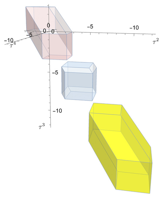
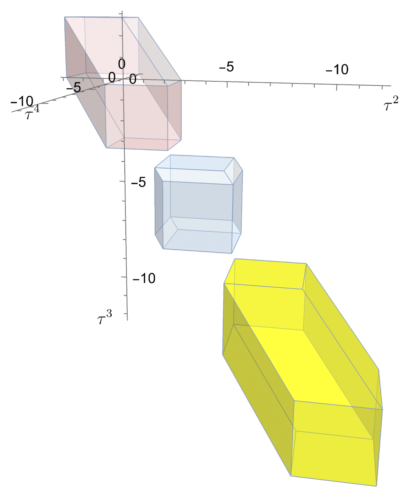
The dodecahedron contracts longitudinally along the main bisectrix as we approach ${\tau }_v^1=-{\displaystyle \frac{4}{\sqrt{3}\gamma \beta }}$ from left and right, where it is smallest. Figure 1 shows the shadow dodecahedron for $\beta ={\displaystyle \frac{1}{2}}$ at the endpoints and midpoint of the interval4 of ${\tau }^1\in [-{\displaystyle \frac{8}{\sqrt{3}\gamma \beta }},0]$, that is, for ${\tau }^1=-8$, ${\tau }^1=-4$ and ${\tau }^1=0$. At the midpoint (${\tau }_v^1=-4$), the dodecahedron is smallest.

Figure 1. The shadow dodecahedron for $\beta ={\displaystyle \frac{1}{2}}$ at ${\tau }^1=0$ (purple), ${\tau }^1=-4$ (blue) and ${\tau }^1=-8$ (yellow).

We can study the motion of the shadow dodecahedron along the main bisectrix through the motion of the spatial circumcentre of the tetrahedron formed by the four satellites, whose world line (${\gamma }_c$), parametrized with the proper time of emitter 1 (${\tau }^1$), is expressed as follow:

$$\begin{array}{cc}\hfill {\gamma }_c=& \gamma {\tau }^{1}u+{\displaystyle \frac{{\omega }_c}{\sqrt{3}}}(1,1,1),\hfill \\ \hfill {\omega }_c=& {\displaystyle \frac{\beta \gamma {\tau }^1(6+\sqrt{3}\beta \gamma {\tau }^1)}{8+2\sqrt{3}\beta \gamma {\tau }^1}}.\hfill \end{array}$$

(15)

As mentioned in the previous section, this world line is degenerate at ${\tau }^1={\tau }_v^1$, when all four emitters are spatially coplanar.

We can now write the trajectory of the spatial circumcentre on the grid (${\mathcal{T}}_1$):

$$\begin{array}{c}{S}_c=(f_c,f_c,f_c),\\ \begin{array}{cc}\hfill f_c\left({\tau }^1\right)& =\gamma {\tau }^1-{\displaystyle \frac{\sqrt{{\mathrm{\Delta }}_c}}{2\left(3\mathrm{\Gamma }+4\right)}},\hfill \\ \hfill {\mathrm{\Delta }}_c& =81{\mathrm{\Gamma }}^4+(36\sqrt{3}+324){\mathrm{\Gamma }}^3+(120\sqrt{3}+432){\mathrm{\Gamma }}^2+(96\sqrt{3}+288)\mathrm{\Gamma }+192.\hfill \end{array}\end{array}$$

In the ${\mathcal{T}}_1$ grid, the spatial circumcentre described by world line ${\gamma }_c$ (15) moves along the bisectrix of the grid. We can determine whether it lies inside the shadow dodecahedron for any ${\tau }^1$ by comparing its coordinates with those of vertices $V_1$ and $V_2$, the end vertices on the bisectrix. It lies inside the dodecahedron for any ${\tau }^1>{\tau }_b^1$ and ${\tau }^1<{\tau }_a^1$, where ${\tau }_a^1$ and ${\tau }_b^1$ are the ${\tau }^1$ coordinates of the two intersection points of $y_{\gamma }\left({\tau }^1\right)$ and $g_c\left({\tau }^1\right)\equiv {\displaystyle \frac{{\mathrm{\Delta }}_c}{4{\left(3\mathrm{\Gamma }+4\right)}^2}}$. In the interval of $[{\tau }_a^1,{\tau }_b^1]$, function $g_c\left({\tau }^1\right)$ diverges at ${\tau }^1={\tau }_v^1$, when the four emitters are spatially coplanar (see Section 3.2).

3.4. Interpreting the RPS Solution

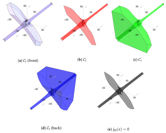
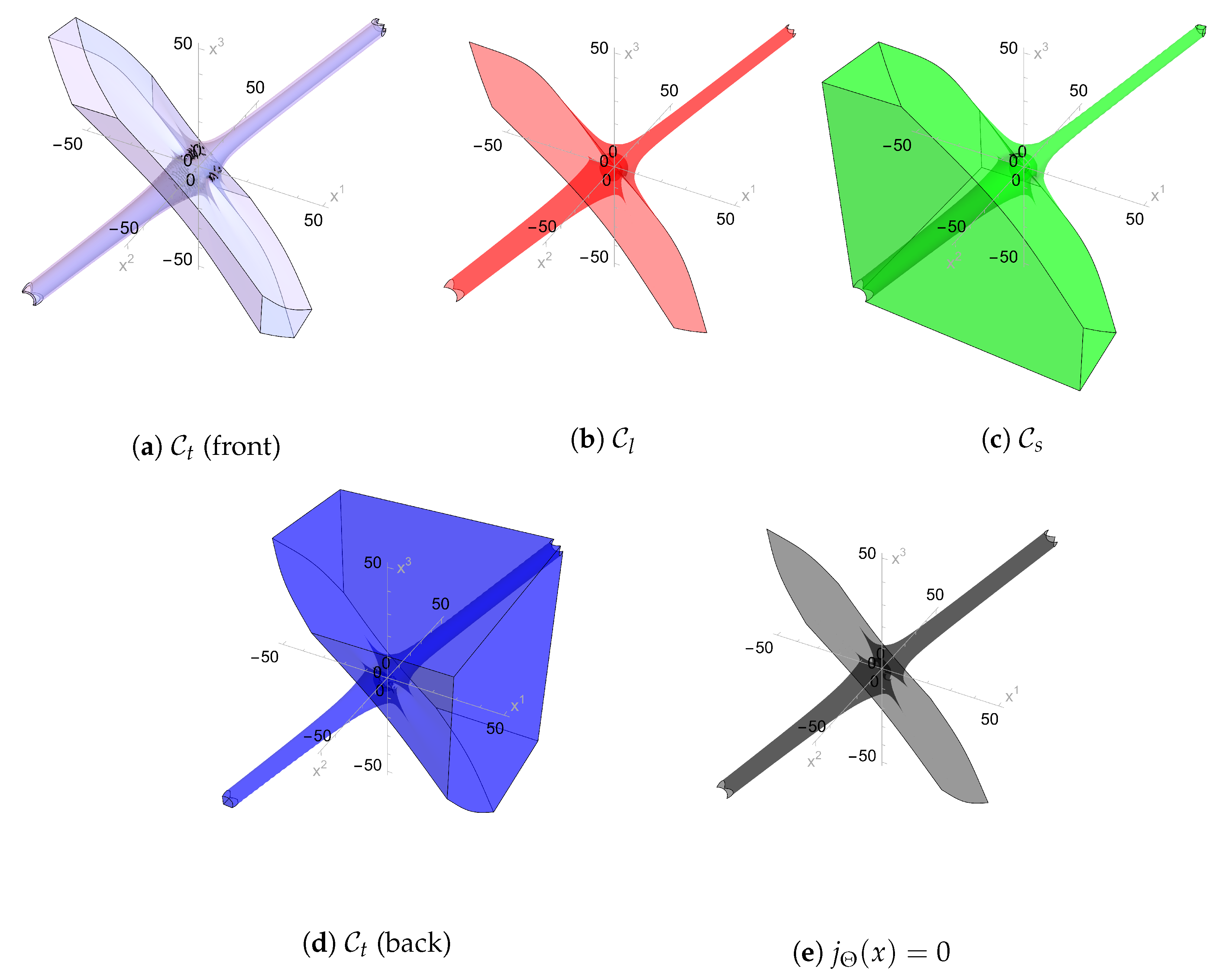
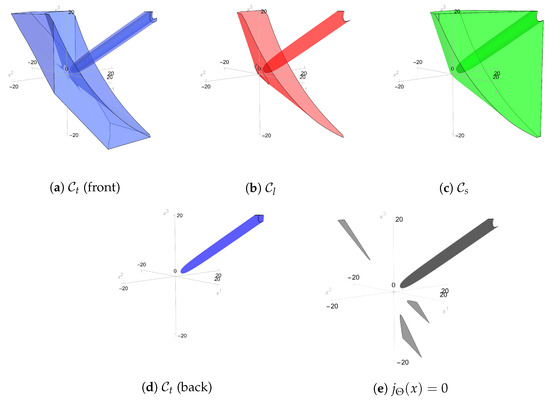
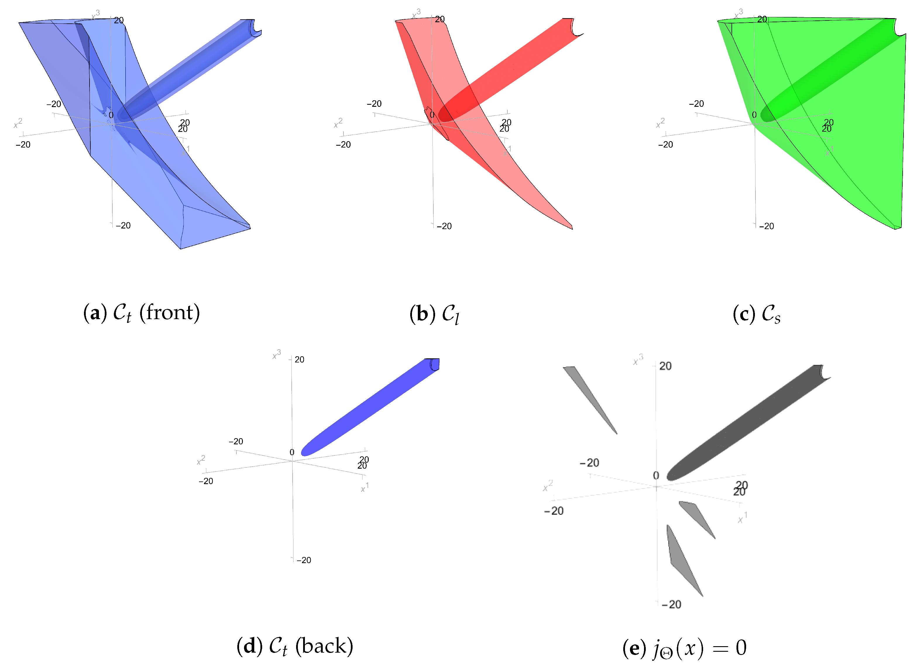
We now represent the characteristic regions of the RPS solution in Cartesian coordinates for this case, depending on the causal character of the configuration vector ($\chi$). Unlike the static situation [9], these regions change with every inertial instant ($x^0$) for a given velocity ($\beta$). But, as in the static situation, for every $x^0$, the RPS solution is defined in the whole Euclidean space $\{x^1,x^2,x^3\}$. Figure 2 shows these regions and the region expressed as $j_{\mathrm{\Theta }}\left(x\right)=0$, where the Jacobian determinant of the transformation from inertial to emission coordinates vanishes, for $\beta ={\displaystyle \frac{1}{2}}$ and $x^0=1$.

Figure 2. Representation of the emission-configuration regions at $x^0=1$ for an RPS with one inertial emitter moving with $\beta ={\displaystyle \frac{1}{2}}$ and three static emitters. Emission configuration regions ${\mathcal{C}}_s$ (space-like), ${\mathcal{C}}_l$ (light-like) and ${\mathcal{C}}_t$ (time-like) are coloured in green, red and blue, respectively. The 3-surface where $j_{\mathrm{\Theta }}\left(x\right)$ vanishes is shown in black.

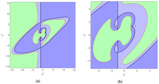
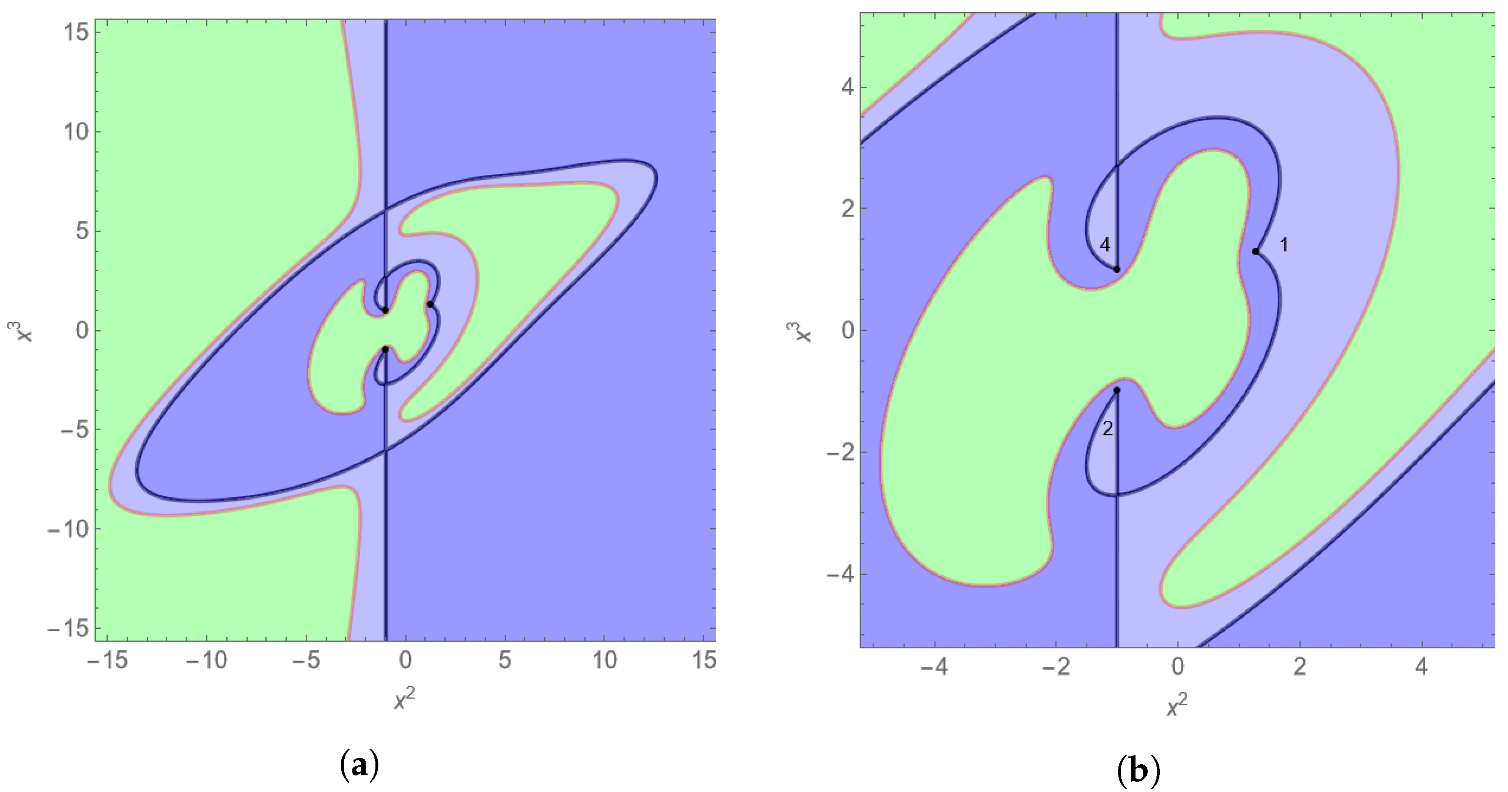
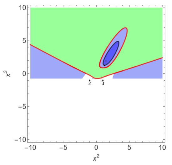
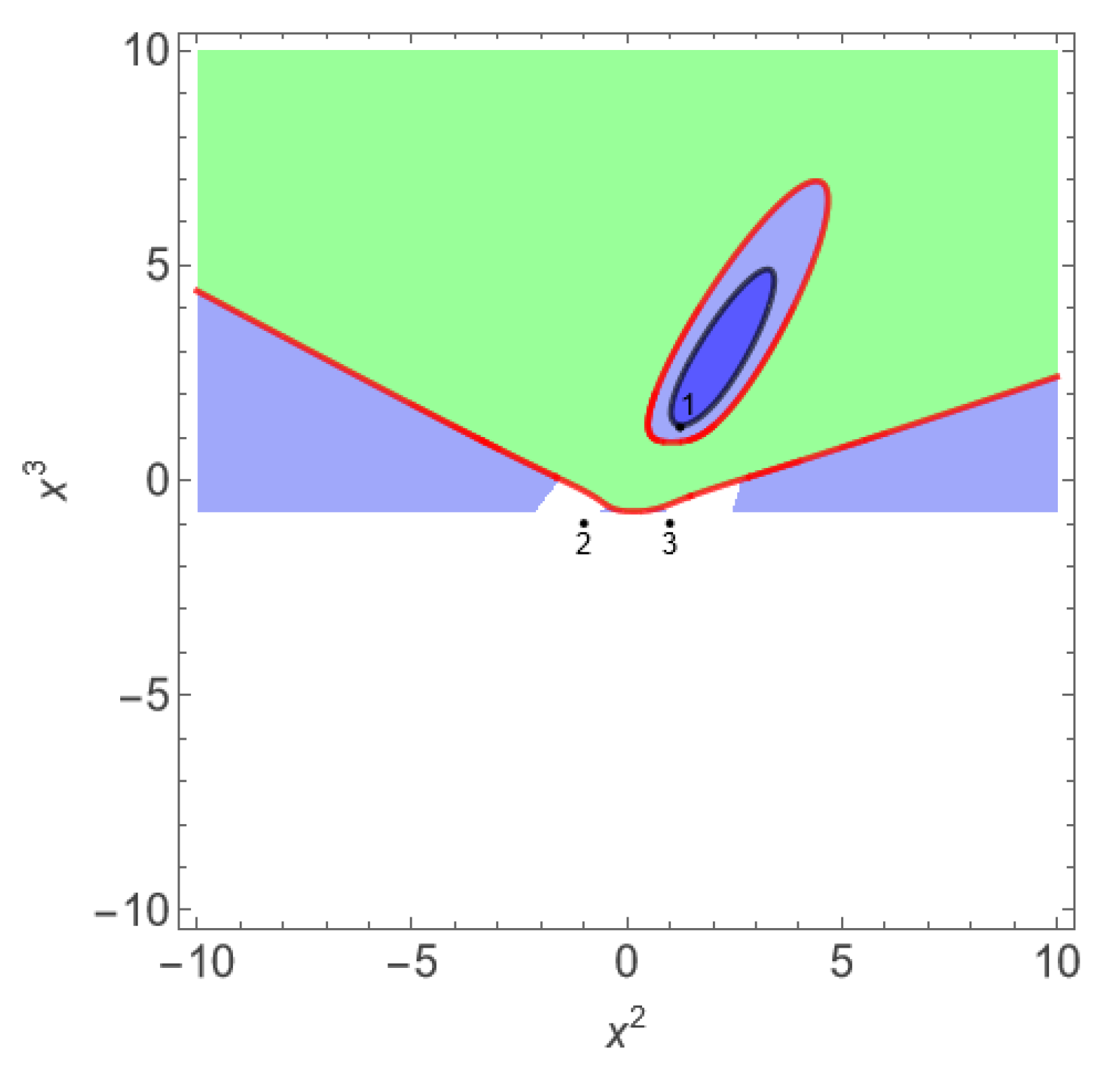
Figure 3 includes a two-dimensional slice of the emission-configuration regions shown in Figure 2, through the plane containing emitters 1, 2 and 4 at $x^0=1$ ($\beta ={\displaystyle \frac{1}{2}}$). The intersection with $j_{\mathrm{\Theta }}\left(x\right)=0$ is also represented. We can see that around the satellites, the configuration regions are interlaced with each other.

Figure 3. Slice of the emission-configuration regions (shown in Figure 2) through the plane containing emitters 1, 2 and 4 at $x^0=1$ ($\beta ={\displaystyle \frac{1}{2}}$). The color convention is the same as in Figure 2. Black points represent satellites, as indicated. (a) Slice of the emission-configuration regions. (b) Zoom in of the region containing satellites 1, 2 and 4.

To remark on the essential properties of the RPS solution in this example, we consider the inertial coordinate location of those users whose emission coordinates satisfy the restrictions expressed as ${\tau }^1=-\sigma ,{\tau }^2={\tau }^3={\tau }^4=\sigma$. We start by computing the configuration covector (1) using (10):

$${\chi }_{\mu }=-4\left(\sqrt{3}\gamma \beta \sigma -4,\left(1+\gamma \right)\sigma ,\left(1+\gamma \right)\sigma ,\left(1+\gamma \right)\sigma \right).$$

(16)

To calculate the particular solution ($y_{*}$), we first compute the configuration bivector (H) using (10), (11), (8) and (7). Setting the transversal vector as $\xi =u$, Equation (6) yields:

$$y_{{*}_{\mu }}={\displaystyle \frac{4}{D}}\left(0,{\sigma }^2(1+\gamma )+2\sqrt{3}\gamma \beta \sigma -4,{\sigma }^2(1+\gamma )+2\sqrt{3}\gamma \beta \sigma -4,{\sigma }^2(1+\gamma )+4\right),$$

(17)

with $D=4(\sqrt{3}\gamma \beta \sigma -4)$. With this choice of $\xi$, the transversality condition restricts this solution to $\{\sigma \in \mathbb{R}|\sigma \ne -{\tau }_v^1={\displaystyle \frac{4}{\sqrt{3}\gamma \beta }}\}$. As stated earlier, at ${\tau }^1={\tau }_v^1$, all four emitters are spatially coplanar, leading to a degenerate situation.5

The solution (5) reads as follows:

$$\begin{array}{c}\hfill x^{\mu }(-\sigma ,\sigma ,\sigma ,\sigma )=(\sigma ,-1,-1,1)+y_{*}-{\displaystyle \frac{{\lambda }_1}{{\lambda }_2}}\chi ,\end{array}$$

(18)

with polynomial functions of $\sigma$, i.e.,

$$\begin{array}{cc}\hfill {\lambda }_1& =4\left(3{(1+\gamma )}^2{\sigma }^4+8\sqrt{3}\gamma \beta (1+\gamma ){\sigma }^3+8(3{\gamma }^2-\gamma -4){\sigma }^2-32\sqrt{3}\gamma \beta \sigma +48\right),\hfill \\ \hfill {\lambda }_2& =D\left(-12{(1+\gamma )}^2{\sigma }^3-16\sqrt{3}\gamma \beta (1+\gamma ){\sigma }^2+16(1+\gamma )\sigma +\widehat{ϵ}D\sqrt{{\mathrm{\Delta }}_{\sigma }}\right),\hfill \\ \hfill {\mathrm{\Delta }}_{\sigma }& ={\displaystyle \frac{{\lambda }_1}{4}}-8{(1+\gamma )}^2{\sigma }^2.\hfill \end{array}$$

In this case, $q_1=-\sigma (\gamma +1)$, $q_2=q_3=0$, and the emission-reception conditions (12) are reduced to the following:

$$\left|\sigma \right|<{\displaystyle \frac{1}{\gamma +1}}\sqrt{({\gamma }^2-1){\sigma }^2-{\displaystyle \frac{8\gamma \beta }{\sqrt{3}}}\sigma +8},$$

(19)

taking into account (13), which is equivalently written as

$$P\left(\sigma \right)\equiv {\sigma }^2+{\displaystyle \frac{4}{\sqrt{3}}}\sqrt{{\displaystyle \frac{\gamma -1}{\gamma +1}}}\sigma -{\displaystyle \frac{4}{\gamma +1}}<0.$$

(20)

The roots of $P\left(\sigma \right)=0$, i.e.,

$${\sigma }_{\pm }={\displaystyle \frac{2}{\sqrt{3}}}{\displaystyle \frac{1}{\sqrt{\gamma +1}}}\left(-\sqrt{\gamma -1}\pm \sqrt{\gamma +2}\right),$$

(21)

provide the limiting values for $\sigma$ imposed by the emission-reception conditions.

Table 1 shows the result of setting $\beta ={\displaystyle \frac{1}{2}}$ for different values of $\sigma$. In this particular case, the emission-reception condition (19) imposes

$$-1.71\approx {\displaystyle \frac{2}{3}}(-2\sqrt{3}-\sqrt{6(\sqrt{3}-1)}+3)<\sigma <{\displaystyle \frac{2}{3}}(-2\sqrt{3}+\sqrt{6(\sqrt{3}-1)}+3)\approx 1.09.$$

Table 1. RPS solution for users with ${\tau }^1=-\sigma ,{\tau }^2=\sigma ,{\tau }^3=\sigma ,{\tau }^4=\sigma$ for different values of $\sigma$.

$\mathit{\sigma }$	${\mathit{\chi }}^2$	${\mathbf{\Delta }}_{\mathit{\sigma }}$	${\mathit{x}}^0$	${\mathit{x}}^1={\mathit{x}}^2={\mathit{x}}^3$	Emission Solutions
${\displaystyle \frac{1}{2}}$	<0	>0	${\displaystyle \frac{9}{44}}\left(5\sqrt{3}+3\right)$	$-{\displaystyle \frac{1}{44}}\left(9\sqrt{3}+23\right)$	$\widehat{ϵ}=-1$ One emission solution
$2(1-\sqrt{3})$	0	>0	$-{\displaystyle \frac{3}{2}}\left(\sqrt{3}-3\right)$	${\displaystyle \frac{1}{2}}\left(\sqrt{3}+1\right)$	$\widehat{ϵ}=-1$ One emission solution
$-{\displaystyle \frac{3}{2}}$	>0	>0	${\displaystyle \frac{5}{4}}(5\sqrt{3}+9)$	${\displaystyle \frac{3}{4}}(5\sqrt{3}+9)$	$\widehat{ϵ}=1$
			${\displaystyle \frac{49}{524}}(17\sqrt{3}-9)$	${\displaystyle \frac{3}{524}}(49\sqrt{3}+159)$	$\widehat{ϵ}=-1$
					Two emission solutions

(i)

For $\sigma ={\displaystyle \frac{1}{2}}$, the emitter configuration is space-like at

$x^{\mu }={\displaystyle \frac{1}{44}}\left(9\left(5\sqrt{3}+3\right),-\left(9\sqrt{3}+23\right),-\left(9\sqrt{3}+23\right),-\left(9\sqrt{3}+23\right)\right)$, which is the sole emission solution (with $\widehat{ϵ}=-1$). The solution with $\widehat{ϵ}=1$ is a reception solution.

(ii)

For $\sigma =2(1-\sqrt{3})$, the emitter configuration is light-like at

$x^{\mu }={\displaystyle \frac{1}{2}}\left(-3\left(\sqrt{3}-3\right),\left(\sqrt{3}+1\right),\left(\sqrt{3}+1\right),\left(\sqrt{3}+1\right)\right)$, which is the sole emission solution (with $\widehat{ϵ}=-1$). The solution with $\widehat{ϵ}=1$ is degenerate.

(iii)

For $\sigma =-{\displaystyle \frac{3}{2}}$, the emitter configuration is time-like at

$x_{+}^{\mu }={\displaystyle \frac{(5\sqrt{3}+9)}{4}}\left(5,3,3,3\right)$ and

$x_{-}^{\mu }={\displaystyle \frac{1}{524}}\left(49(17\sqrt{3}-9),3(49\sqrt{3}+159),3(49\sqrt{3}+159),3(49\sqrt{3}+159)\right)$, both being emission solutions (with $\widehat{ϵ}=1$ and $\widehat{ϵ}=-1$, respectively); $x_{-}\left(x_{+}\right)$ is in the front (back) emission coordinate domain.

The main results obtained in this section can be particularized by setting $\beta =0$ to describe the case where all four emitters are static and spatially form a regular tetrahedron (see [9] for the static case in which the emitters form an orthogonal tetrahedron).

4. RPS with One Hyperbolic and Three Static Emitters

In this example, we consider that emitters $2, 3$ and 4 are static. Emitter 1 is moving in hyperbolic motion with constant proper acceleration of $\alpha >0$ along the bisectrix $(1,1,1)$ in such a way that at ${\tau }^1=0$, the four emitters spatially form a regular tetrahedron. As ${\tau }^1\to \pm \infty$, its spatial position tends toward $+\infty$ along the main bisectrix.

4.1. Emitters’ World Lines and Emission/Reception Conditions

World lines with respect to the inertial observer (u) are expressed as follows:

$$\begin{array}{cccc}\hfill {\gamma }_1=& {\displaystyle \frac{\gamma \left({\tau }^1\right)\beta \left({\tau }^1\right)}{\alpha }}u+\left[{\displaystyle \frac{\gamma \left({\tau }^1\right)-1}{\sqrt{3}\alpha }}+1\right](1,1,1),\hfill & \hfill {\gamma }_2& ={\tau }^{2}u+(1,-1,-1),\hfill \\ \hfill {\gamma }_3=& {\tau }^{3}u+(-1,1,-1),\hfill & \hfill {\gamma }_4& ={\tau }^{4}u+(-1,-1,1),\hfill \end{array}$$

where $\gamma \left({\tau }^1\right)=cosh\left(\alpha {\tau }^1\right)$ and $\beta \left({\tau }^1\right)=tanh\left(\alpha {\tau }^1\right)$. Expressing the coordinate time in seconds, the proper acceleration ($\alpha$) is expressed in $s^{-1}$. We consider that the proper times of emitters 2, 3 and 4 are synchronised at their common origin of ${\tau }^2={\tau }^3={\tau }^4=0$ and that the proper time of emitter 1 is synchronised with theirs at ${\tau }^1=0$. The distance covered by emitter 1 in one second of coordinate time ($\mathrm{\Delta }{x}^0=1s$), starting from zero coordinate time when it is at rest with respect to the inertial observer ($\mathrm{\Delta }{\tau }^1={\displaystyle \frac{arcsinh\left(\alpha \mathrm{\Delta }{x}^0\right)}{\alpha }}={\displaystyle \frac{arcsinh\left(\alpha \right)}{\alpha }}$), is $d_1={\displaystyle \frac{cosh\left(\alpha \mathrm{\Delta }{\tau }^1\right)-1}{\alpha }}ls$.6

Defining

$$\begin{array}{cc}\hfill \mathrm{\Phi }\left({\tau }^1\right)=& {\displaystyle \frac{\gamma \left({\tau }^1\right)\beta \left({\tau }^1\right)}{\alpha }}={\displaystyle \frac{sinh\left(\alpha {\tau }^1\right)}{\alpha }},\mathrm{\Sigma }\left({\tau }^1\right)={\displaystyle \frac{\gamma \left({\tau }^1\right)-1}{\sqrt{3}\alpha }},\hfill \\ \hfill q_1=& \mathrm{\Phi }-{\tau }^4,q_2={\tau }^2-{\tau }^4,q_3={\tau }^3-{\tau }^4,\hfill \end{array}$$

one obtains the following position vectors with respect to the fourth emitter, i.e., $e_a={\gamma }_a-{\gamma }_4$, $a=1, 2, 3$:

$$\begin{array}{c}\hfill e_1=q_{1}u+(\mathrm{\Sigma }+2,\mathrm{\Sigma }+2,\mathrm{\Sigma }),e_2=q_{2}u+(2,0,-2),e_3=q_{3}u+(0,2,-2),\end{array}$$

(22)

along with the following world-functions (${\mathrm{\Omega }}_a=\frac{1}{2}{\left(e_a\right)}^2$, $a=1, 2, 3$):

$$\begin{array}{c}\hfill {\mathrm{\Omega }}_1=\frac{1}{2}\left(2{(\mathrm{\Sigma }+2)}^2+{\mathrm{\Sigma }}^2-q_1^2\right),{\mathrm{\Omega }}_2=\frac{1}{2}(8-q_2^2),{\mathrm{\Omega }}_3=\frac{1}{2}(8-q_3^2).\end{array}$$

(23)

The emission/reception conditions of $e_a^2>0$ and ${(e_a-e_b)}^2>0$ read as follows:

$$\begin{array}{cc}\hfill |\mathrm{\Phi }-{\tau }^4|& <\sqrt{2{(\mathrm{\Sigma }+2)}^2+{\mathrm{\Sigma }}^2},|{\tau }^2-{\tau }^4|<\sqrt{8},\left|{\tau }^3-{\tau }^4\right|<\sqrt{8},\hfill \\ \hfill \left|\mathrm{\Phi }-{\tau }^2\right|<& \sqrt{2{(\mathrm{\Sigma }+2)}^2+{\mathrm{\Sigma }}^2},|\mathrm{\Phi }-{\tau }^3|<\sqrt{2{(\mathrm{\Sigma }+2)}^2+{\mathrm{\Sigma }}^2},\left|{\tau }^2-{\tau }^3\right|<\sqrt{8}.\hfill \end{array}$$

4.2. Emitters’ Trajectories on the Grid ($\mathcal{T}$)

In this case, the equations to obtain the ${\tau }^1$ coordinate of trajectories $S_2$, $S_3$ and $S_4$ (${({\gamma }_i-{\gamma }_1)}^2=0$, $i=2,3,4$) are expressed as follows:

$$\begin{array}{cc}\hfill & A\sqrt{t^2+1}+B_{i}t+C_i=0,t=sinh\left(\alpha {\tau }^1\right),\hfill \\ \hfill & A={\displaystyle \frac{6}{\alpha }}-8\sqrt{3},B_i=-6{\tau }^i,C_i=3\alpha {\left({\tau }^i\right)}^2-24\alpha -A,i=2,3,4.\hfill \end{array}$$

(24)

For $\alpha ={\displaystyle \frac{\sqrt{3}}{4}}\equiv {\alpha }_0$ ($A=0$), the solution to (24) is

$$\begin{array}{c}\hfill v_0\left({\tau }^i\right)={\displaystyle \frac{4}{\sqrt{3}}}arcsinh\left({\displaystyle \frac{\sqrt{3}\left({\left({\tau }^i\right)}^2-8\right)}{8{\tau }^i}}\right),i=2,3,4.\end{array}$$

(25)

Solution $v_0$ is valid for ${\tau }^i\ne 0$. It will be an emission solution iff the corresponding inertial time at the emission event, i.e., $\mathrm{\Phi }\left(v_0\right)$, is less than the inertial time at the reception event, i.e., ${\tau }^i$,${\displaystyle \frac{\sqrt{3}\left({\left({\tau }^i\right)}^2-8\right)}{8{\tau }^i}}<{\tau }^i$, that is, iff ${\tau }^i>0$.

For $\alpha \ne {\alpha }_0$, the solution of (24) is

$$\begin{array}{cc}\hfill v_{\alpha }\left({\tau }^i\right)=& {\displaystyle \frac{1}{\alpha }}arcsinh\left(D_i\right),D_i={\displaystyle \frac{B_i{C}_i+\rho \sqrt{A^2(B_i^2+C_i^2-A^2)}}{A^2-B_i^2}},\rho =\pm 1,i=2,3,4.\hfill \end{array}$$

(26)

The two solutions included in (26), depending on the sign ($\rho$), originate from the solution process of the square-root equation (24) and therefore have to satisfy the additional condition of ${\displaystyle \frac{B_i}{A}}{D}_i+{\displaystyle \frac{C_i}{A}}<0$. Additionally, solution $v_{\alpha }$ is valid for ${\tau }^i\ne \pm \left({\displaystyle \frac{1}{\alpha }}-{\displaystyle \frac{4}{\sqrt{3}}}\right)$ and will be an emission solution iff $D_i<{\tau }^i$.

$v\left(\tau \right)$ denotes solution (25) or (26), depending on the value of $\alpha$, and supposing the conditions for each of these solutions are satisfied, we obtain the following trajectories ($S_A$) on the grid ($\mathcal{T}$):

$$\begin{array}{c}\hfill \begin{array}{cc}\hfill S_1\left(\tau \right)& :\left(\tau ,\mathrm{\Phi }-\sqrt{2{(\mathrm{\Sigma }+2)}^2+{\mathrm{\Sigma }}^2},\mathrm{\Phi }-\sqrt{2{(\mathrm{\Sigma }+2)}^2+{\mathrm{\Sigma }}^2},\mathrm{\Phi }-\sqrt{2{(\mathrm{\Sigma }+2)}^2+{\mathrm{\Sigma }}^2}\right),\hfill \\ \hfill S_2\left(\tau \right)& :\left(v\left(\tau \right),\tau ,\tau -\sqrt{8},\tau -\sqrt{8}\right),\hfill \\ \hfill S_3\left(\tau \right)& :\left(v\left(\tau \right),\tau -\sqrt{8},\tau ,\tau -\sqrt{8}\right),\hfill \\ \hfill S_4\left(\tau \right)& :\left(v\left(\tau \right),\tau -\sqrt{8},\tau -\sqrt{8},\tau \right),\hfill \end{array}\end{array}$$

(27)

with $\mathrm{\Phi }\left(\tau \right)={\displaystyle \frac{sinh\left(\alpha \tau \right)}{\alpha }}$ and $\mathrm{\Sigma }\left(\tau \right)={\displaystyle \frac{\gamma \left(\tau \right)-1}{\sqrt{3}\alpha }}$.

4.3. Shadow Dodecahedron

We can write the coordinates of the 14 vertices of the shadow dodecahedron on the grid (${\mathcal{T}}_1\equiv \left[{\tau }^2\right]\times \left[{\tau }^3\right]\times \left[{\tau }^4\right]$), with these coordinates depending on ${\tau }^1$ as follows:

$$\begin{array}{cc}{V}_1=(K_{+},K_{+},K_{+}),\hfill & V_2=(K_{-},K_{-},K_{-}),\hfill \\ V_3=(K_{+}-\sqrt{8},K_{+},K_{+}),\hfill & V_4=(K_{+},K_{+}-\sqrt{8},K_{+}),\hfill \\ V_5=(K_{+},K_{+},K_{+}-\sqrt{8}),\hfill & V_6=(K_{-}+\sqrt{8},K_{-},K_{-}),\hfill \\ V_7=(K_{-},K_{-}+\sqrt{8},K_{-}),\hfill & V_8=(K_{-},K_{-},K_{-}+\sqrt{8}),\hfill \\ V_9=(K_{+}-\sqrt{8},K_{+}-\sqrt{8},K_{+}),\hfill & V_{10}=(K_{+},K_{+}-\sqrt{8},K_{+}-\sqrt{8}),\hfill \\ V_{11}=(K_{+}-\sqrt{8},K_{+},K_{+}-\sqrt{8}),\hfill & V_{12}=(K_{-}+\sqrt{8},K_{-}+\sqrt{8},K_{-}),\hfill \\ V_{13}=(K_{-},K_{-}+\sqrt{8},K_{-}+\sqrt{8}),\hfill & V_{14}=(K_{-}+\sqrt{8},K_{-},K_{-}+\sqrt{8}),\hfill \end{array}$$

with $K_{\pm }\left({\tau }^1\right)\equiv \mathrm{\Phi }\pm \sqrt{2{(\mathrm{\Sigma }+2)}^2+{\mathrm{\Sigma }}^2}$. Of these 14 vertices, only one coincides with a satellite trajectory on the grid (${\mathcal{T}}_1$)—namely, $V_2$ with the trajectory of satellite 1.

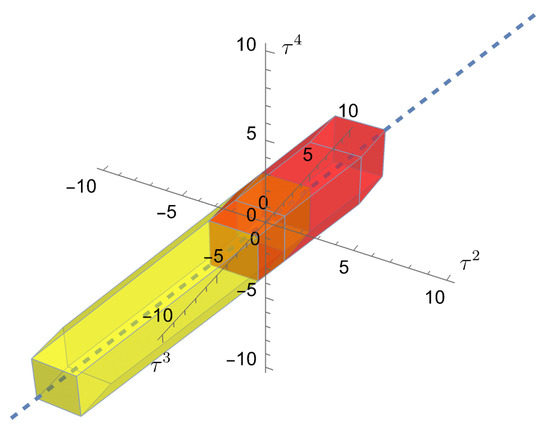
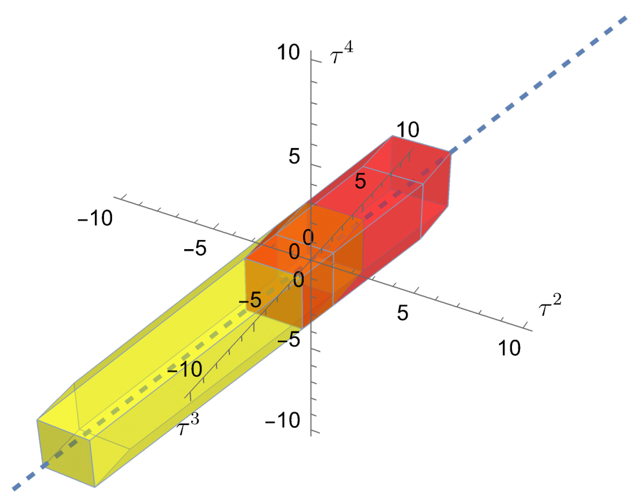
To describe the motion of the dodecahedron on the grid (${\mathcal{T}}_1$) as ${\tau }^1\to \pm \infty$, note that vertices $V_1$ and $V_2$, the endpoints on the main bisectrix, satisfy ${lim}_{{\tau }^1\to -\infty }{V}_1=l_{\alpha }$ and ${lim}_{{\tau }^1\to \infty }{V}_2=-l_{\alpha }$, with $l_{\alpha }=(-{\displaystyle \frac{1}{\alpha }}+{\displaystyle \frac{4}{\sqrt{3}}})(1,1,1)$. The translational motion is therefore restricted by this limit: as ${\tau }^1\to -\infty$, $V_1$ does not go beyond $l_{\alpha }$, and as ${\tau }^1\to \infty$, $V_2$ does not go beyond $-l_{\alpha }$. Its longitudinal deformation, however, increases as $|{\tau }^1|\to \infty$. At ${\tau }^1=0$, the dodecahedron is smallest. Figure 4 shows the shadow dodecahedron for $\alpha =1$ at ${\tau }^1=-2$ and ${\tau }^1=1$.

Figure 4. The shadow dodecahedron on the grid (${\mathcal{T}}_1$) for $\alpha =1$ at ${\tau }^1=-2$ (yellow and orange overlap) and ${\tau }^1=1$ (red and orange overlap). The main bisectrix is also shown (dashed line).

4.4. Interpreting the RPS Solution

We can represent the characteristic regions of the RPS solution in Cartesian coordinates for this example, depending on the causal character of the configuration vector ($\chi$). Figure 5 shows these regions and the region where the Jacobian determinant of the transformation from inertial to emission coordinates vanishes, i.e., $j_{\mathrm{\Theta }}\left(x\right)=0$, for $\alpha =1$ and $x^0=1$. As in the previous example involving inertial motion, these regions change with every inertial instant ($x^0$) for a given proper acceleration ($\alpha$). However, unlike that example, for a given $x^0$, the RPS solution is not defined for the whole Euclidean space. Due to the hyperbolic motion of emitter 1, there are space-time regions for which there are no (emission) solutions to the null propagation equation (${(x-{\gamma }_1)}^2=0$).

Figure 5. Representation of the emission-configuration regions at $x^0=1$ for an RPS with one inertial emitter moving in hyperbolic motion with proper acceleration ($\alpha =1$) along the bisectrix $(1,1,1)$ and three static emitters. Emission-configuration regions ${\mathcal{C}}_s$ (space-like), ${\mathcal{C}}_l$ (light-like) and ${\mathcal{C}}_t$ (time-like) are coloured in green, red and blue, respectively. The 3-surface where $j_{\mathrm{\Theta }}\left(x\right)$ vanishes is shown in black.

Figure 6 includes a two-dimensional slice of the emission-configuration regions shown in Figure 5 through the plane containing emitters 1, 2 and 3 at $x^0=1$ ($\alpha =1$). Black points represent satellite trajectories. The intersection with $j_{\mathrm{\Theta }}\left(x\right)=0$ is also represented.

Figure 6. Slice of the emission-configuration regions (shown in Figure 5) through the plane containing emitters 1, 2 and 3 at $x^0=1$ ($\alpha =1$). The color convention is the same as in Figure 5. Black points represent the satellites, as indicated. In the white region, the RPS solution is not defined.

To remark on the essential properties of the RPS solution in this hyperbolic case, we consider the inertial coordinate location of those users whose emission coordinates satisfy the restrictions of $\mathrm{\Phi }\left({\tau }^1\right)=-\sigma$ and ${\tau }^2={\tau }^3={\tau }^4=\sigma$, for which

$${\chi }_{\mu }=-8\left(2+{\displaystyle \frac{\sqrt{3}}{2\alpha }}(\sqrt{{\alpha }^2{\sigma }^2+1}-1),\sigma ,\sigma ,\sigma \right),$$

(28)

where we use (22) and (1). To calculate the particular solution ($y_{*}$), we first compute H using (22), (23), (8) and (7). Then, setting the transversal vector as $\xi =u$, Equation (6) yields the following:

$$\begin{array}{c}{y}_{{*}_{\mu }}={\displaystyle \frac{2}{{\alpha }^{2}D}}\left(0,y_{{*}_1},y_{{*}_2},y_{{*}_3}\right),D=-4\left(4+{\displaystyle \frac{\sqrt{3}}{\alpha }}(\sqrt{{\alpha }^2{\sigma }^2+1}-1)\right),\end{array}$$

(29)

$$\begin{array}{c}\begin{array}{cc}\hfill y_{{*}_1}& =y_{{*}_2}=3{\alpha }^2{\sigma }^2-(4\sqrt{3}\alpha -2)\sqrt{{\alpha }^2{\sigma }^2+1}-8{\alpha }^2+4\sqrt{3}\alpha -2,\hfill \\ \hfill y_{{*}_3}& =3{\alpha }^2{\sigma }^2+2\sqrt{{\alpha }^2{\sigma }^2+1}+8{\alpha }^2-2.\hfill \end{array}\end{array}$$

(30)

With this choice of $\xi$, the transversality condition imposes no restriction on this solution ($D\ne 0$ for any $\{\alpha ,\sigma \}$). Taking into account (9), the solution reads as follows:

$$\begin{array}{c}{x}^{\mu }(-\sigma ,\sigma ,\sigma ,\sigma )=(\sigma ,-1,-1,1)+y_{*}-{\displaystyle \frac{{\lambda }_1}{{\lambda }_2}}\chi ,\\ \begin{array}{cc}\hfill {\lambda }_1& =27{\alpha }^4{\sigma }^4+4{\alpha }^2{\sigma }^2(-6+12{\alpha }^2+9\sqrt{{\alpha }^2{\sigma }^2+1}+4\sqrt{3}\alpha (1-3\sqrt{{\alpha }^2{\sigma }^2+1}))\hfill \\ & +8(-3+8\sqrt{3}\alpha -28{\alpha }^2+16\sqrt{3}{\alpha }^3)\sqrt{{\alpha }^2{\sigma }^2+1}+8(3-8\sqrt{3}\alpha +28{\alpha }^2-16\sqrt{3}{\alpha }^3+24{\alpha }^4),\hfill \\ \hfill {\lambda }_2& =-2{\alpha }^{2}D\left(18{\alpha }^2{\sigma }^3-4\sigma [3(1-\sqrt{{\alpha }^2{\sigma }^2+1})+4\alpha (\alpha +\sqrt{3}(\sqrt{{\alpha }^2{\sigma }^2+1}-1))]-\widehat{ϵ}{\alpha }^{2}D\sqrt{{\mathrm{\Delta }}_{\sigma }}\right),\hfill \\ \hfill {\mathrm{\Delta }}_{\sigma }& ={\displaystyle \frac{{\lambda }_1}{16{\alpha }^4}}-8{\sigma }^2.\hfill \end{array}\end{array}$$

(31)

In this case, the emission-reception conditions are reduced to the following:

$$\left|\sigma \right|<{\displaystyle \frac{1}{2}}\sqrt{{\sigma }^2+{\displaystyle \frac{2}{3{\alpha }^2}}(4\sqrt{3}\alpha -3)(\sqrt{{\alpha }^2{\sigma }^2+1}-1)+8}.$$

(32)

Table 2 shows the result of setting $\alpha =1$ for different values of $\sigma$. In this particular case, the previous emission-reception condition imposes

$\left|\sigma \right|<{\displaystyle \frac{2}{3}}\sqrt{{\displaystyle \frac{1}{3}}(-10\sqrt{3}+\sqrt{838-424\sqrt{3}}+32)}\approx 1.92$.

(i)

For $\tau ={\displaystyle \frac{3}{4}}$, the emitter configuration is space-like at

$x^{\mu }={\displaystyle \frac{1}{1448}}\left(1648\sqrt{3}+821,-5(103\sqrt{3}+40),-5(103\sqrt{3}+40),-5(103\sqrt{3}+40)\right)$, which is the sole emission solution (with $\widehat{ϵ}=-1$). The solution with $\widehat{ϵ}=1$ is a reception solution.

(ii)

For $\tau ={\displaystyle \frac{2}{9}}\left(-4\sqrt{3}-\sqrt{21-6\sqrt{3}}+3\right)\approx -1.60$, the emitter configuration is light-like at $x^{\mu }\approx \left(1.81,1.39,1.39,1.39\right)$, which is the sole emission solution (with $\widehat{ϵ}=-1$). The solution with $\widehat{ϵ}=1$ is degenerate.

(iii)

For $\tau =-{\displaystyle \frac{17}{10}}$, the emitter configuration is time-like at $x_{+}^{\mu }\approx (9.63,6.14,6.14,6.14)$ and $x_{-}^{\mu }\approx (1.84,1.48,1.48,1.48)$, both being emission solutions (with $\widehat{ϵ}=1$ and $\widehat{ϵ}=-1$, respectively); $x_{-}\left(x_{+}\right)$ is in the front (back) emission-coordinate domain.

Table 2. RPS solution with $\alpha =1$ for users with $sinh\left({\tau }^1\right)=-\sigma ,{\tau }^2=\sigma ,{\tau }^3=\sigma ,{\tau }^4=\sigma$.

$\mathit{\sigma }$	${\mathit{\chi }}^2$	${\mathbf{\Delta }}_{\mathit{\sigma }}$	${\mathit{x}}^0$	${\mathit{x}}^1={\mathit{x}}^2={\mathit{x}}^3$	Emission Solutions
${\displaystyle \frac{3}{4}}$	<0	>0	${\displaystyle \frac{1}{1448}}\left(1648\sqrt{3}+821\right)$	$-{\displaystyle \frac{5}{1448}}\left(103\sqrt{3}+40\right)$	$\widehat{ϵ}=-1$ One emission solution
≈$-1.60$	0	>0	≈1.81	≈1.39	$\widehat{ϵ}=-1$ One emission solution
$-{\displaystyle \frac{17}{10}}$	>0	>0	≈9.63	$\approx 6.14$	$\widehat{ϵ}=1$
			≈1.84	≈1.48	$\widehat{ϵ}=-1$
					Two emission solutions

Table 2. RPS solution with $\alpha =1$ for users with $sinh\left({\tau }^1\right)=-\sigma ,{\tau }^2=\sigma ,{\tau }^3=\sigma ,{\tau }^4=\sigma$.

$\mathit{\sigma }$	${\mathit{\chi }}^2$	${\mathbf{\Delta }}_{\mathit{\sigma }}$	${\mathit{x}}^0$	${\mathit{x}}^1={\mathit{x}}^2={\mathit{x}}^3$	Emission Solutions
${\displaystyle \frac{3}{4}}$	<0	>0	${\displaystyle \frac{1}{1448}}\left(1648\sqrt{3}+821\right)$	$-{\displaystyle \frac{5}{1448}}\left(103\sqrt{3}+40\right)$	$\widehat{ϵ}=-1$ One emission solution
≈$-1.60$	0	>0	≈1.81	≈1.39	$\widehat{ϵ}=-1$ One emission solution
$-{\displaystyle \frac{17}{10}}$	>0	>0	≈9.63	$\approx 6.14$	$\widehat{ϵ}=1$
			≈1.84	≈1.48	$\widehat{ϵ}=-1$
					Two emission solutions

5. RPS with One Static and Three Rotating Emitters

In this example, we consider the spatial configuration of emitters 1, 2 and 3 following uniform circular motion on the $\{x,y\}$ plane at a constant radial distance ($r_0$) and equally spaced at an angle of ${\displaystyle \frac{2\pi }{3}}$, with emitter 4 static at distance d on the z-axis.

5.1. Emitters’ World Lines and Emission/Reception Conditions

If $\omega$ is the constant angular velocity with respect to the inertial observer (u), we can write the world lines as follows:

$$\begin{array}{cc}\hfill {\gamma }_1=& \gamma {\tau }^{1}u+r_0\left(cos\left(\omega \gamma {\tau }^1\right),sin\left(\omega \gamma {\tau }^1\right),0\right),\hfill \\ \hfill {\gamma }_2=& \gamma {\tau }^{2}u+r_0\left(cos(\omega \gamma {\tau }^2-{\displaystyle \frac{2\pi }{3}}),sin(\omega \gamma {\tau }^2-{\displaystyle \frac{2\pi }{3}}),0\right),\hfill \\ \hfill {\gamma }_3=& \gamma {\tau }^{3}u+r_0\left(cos(\omega \gamma {\tau }^3-{\displaystyle \frac{4\pi }{3}}),sin(\omega \gamma {\tau }^3-{\displaystyle \frac{4\pi }{3}}),0\right),{\gamma }_4={\tau }^{4}u+(0,0,d),\hfill \end{array}$$

(33)

where $\gamma ={(1-{\beta }^2)}^{-{\displaystyle \frac{1}{2}}}$ and $\beta =\omega r_0$ ($\omega r_0<1$). The velocity ($\beta$) is expressed as a fraction of the speed of light in vacuum c ($\beta <1$). We consider that the proper times of emitters 1, 2 and 3 are synchronised at their common origin of ${\tau }^1={\tau }^2={\tau }^3=0$ and synchronised with emitter 4 at ${\tau }^4=0$. Expressing the coordinate time in seconds and the spatial coordinates in kilometres, the number of revolutions ($s_1$) completed by emitter 1 in one second of coordinate time, i.e., $\mathrm{\Delta }{x}^0=1s$ ($\mathrm{\Delta }{\tau }^1={\gamma }^{-1}\mathrm{\Delta }{x}^0={\gamma }^{-1}s$), is $s_1\approx {\displaystyle \frac{\beta }{2\pi r_0}}3·{10}^5$, truncated to an integer.7

Defining

$$\begin{array}{c}\hfill q_1={\mathrm{\Gamma }}_1-{\tau }^4,q_2={\mathrm{\Gamma }}_2-{\tau }^4,{\mathrm{\Gamma }}_3-{\tau }^4,{\mathrm{\Gamma }}_a=\gamma {\tau }^a,a=1,2,3,\end{array}$$

one obtains the following position vectors with respect to the fourth emitter, i.e., $e_a={\gamma }_a-{\gamma }_4$, $a=1,2,3$:

$$\begin{array}{cc}\hfill e_1=& q_{1}u+r_0\left(cos\left(\omega {\mathrm{\Gamma }}_1\right),sin\left(\omega {\mathrm{\Gamma }}_1\right),-{\displaystyle \frac{d}{r_0}}\right),\hfill \\ \hfill e_2=& q_{2}u+r_0\left(cos(\omega {\mathrm{\Gamma }}_2-{\displaystyle \frac{2\pi }{3}}),sin(\omega {\mathrm{\Gamma }}_2-{\displaystyle \frac{2\pi }{3}}),-{\displaystyle \frac{d}{r_0}}\right),\hfill \\ \hfill e_3=& q_{3}u+r_0\left(cos(\omega {\mathrm{\Gamma }}_3-{\displaystyle \frac{4\pi }{3}}),sin(\omega {\mathrm{\Gamma }}_3-{\displaystyle \frac{4\pi }{3}}),-{\displaystyle \frac{d}{r_0}}\right),\hfill \end{array}$$

(34)

and the world functions, i.e.,

$$\begin{array}{c}\hfill {\mathrm{\Omega }}_a=\frac{1}{2}(r_0^2+d^2-q_a^2),a=1,2,3.\end{array}$$

(35)

In this example, the emission/reception conditions (3) impose the following:

$$\begin{array}{cc}\hfill |{\mathrm{\Gamma }}_a-{\tau }^4|<& \sqrt{r_0^2+d^2},a=1,2,3,\hfill \\ \hfill |{\mathrm{\Gamma }}_1-{\mathrm{\Gamma }}_2|<& \sqrt{2}{r}_0\sqrt{1+sin(\omega ({\mathrm{\Gamma }}_1-{\mathrm{\Gamma }}_2)+{\displaystyle \frac{\pi }{6}})},\hfill \\ \hfill |{\mathrm{\Gamma }}_1-{\mathrm{\Gamma }}_3|<& \sqrt{2}{r}_0\sqrt{1+sin(\omega ({\mathrm{\Gamma }}_3-{\mathrm{\Gamma }}_1)+{\displaystyle \frac{\pi }{6}})},\hfill \\ \hfill |{\mathrm{\Gamma }}_2-{\mathrm{\Gamma }}_3|<& \sqrt{2}{r}_0\sqrt{1+sin(\omega ({\mathrm{\Gamma }}_2-{\mathrm{\Gamma }}_3)+{\displaystyle \frac{\pi }{6}})}.\hfill \end{array}$$

5.2. Emitters’ Trajectories on the Grid ($\mathcal{T}$)

The emission coordinate (${\tau }^b$) of the a-th emitter($a,b=1,2,3,4$) satisfies the equation expressed as ${({\gamma }_a\left({\tau }^a\right)-{\gamma }_b\left({\tau }^b\right))}^2=0$. Due to the transcendental functions appearing in the world lines of emitters 1, 2 and 3 (33), the ${\tau }^1$, ${\tau }^2$ and ${\tau }^3$ coordinates of the trajectories of emitters 1, 2 and 3 on the grid ($\mathcal{T}$) ($S_1$, $S_2$ and $S_3$) can only be computed numerically by solving the following equations:

$$\begin{array}{cc}\hfill {({\mathrm{\Gamma }}_1-{\mathrm{\Gamma }}_2)}^2=& 2r_0^2\left(1+sin(\omega ({\mathrm{\Gamma }}_1-{\mathrm{\Gamma }}_2)+{\displaystyle \frac{\pi }{6}})\right),\hfill \end{array}$$

(36)

$$\begin{array}{cc}\hfill {({\mathrm{\Gamma }}_3-{\mathrm{\Gamma }}_1)}^2=& 2r_0^2\left(1+sin(\omega ({\mathrm{\Gamma }}_3-{\mathrm{\Gamma }}_1)+{\displaystyle \frac{\pi }{6}})\right),\hfill \end{array}$$

(37)

$$\begin{array}{cc}\hfill {({\mathrm{\Gamma }}_2-{\mathrm{\Gamma }}_3)}^2=& 2r_0^2\left(1+sin(\omega ({\mathrm{\Gamma }}_2-{\mathrm{\Gamma }}_3)+{\displaystyle \frac{\pi }{6}})\right).\hfill \end{array}$$

(38)

Note that Equations (36)–(38) implicitly describe a lineal relationship between ${\tau }^a$ and ${\tau }^b$, i.e., $a,b=1,2,3$. Specifically, the solution of one coordinate in terms of the other is a straight line of unit slope whose intercept has to be computed numerically, so the solution for ${\tau }^2$ of Equation (36) is ${\tau }^2\left({\tau }^1\right)={\tau }^1+m$, with m being the numerical solution8 to the following:

$$m^2={\displaystyle \frac{2r_0^2}{{\gamma }^2}}\left(1+sin(-\omega \gamma m+{\displaystyle \frac{\pi }{6}})\right).$$

(39)

For $r_0=d=1$ and $\omega ={\displaystyle \frac{1}{2}}$$(\gamma ={\displaystyle \frac{2}{\sqrt{3}}})$, $m\approx -1.732$.9

It is clear that the solution for ${\tau }^1$ of Equation (37) is ${\tau }^1\left({\tau }^3\right)={\tau }^3+m$ and that the solution for ${\tau }^3$ of (38) is ${\tau }^3\left({\tau }^2\right)={\tau }^2+m$. Analogously, the solution for ${\tau }^1$ of (36) is ${\tau }^1\left({\tau }^2\right)={\tau }^2+n$, with n being the (negative) numerical solution to the following:

$$n^2={\displaystyle \frac{2r_0^2}{{\gamma }^2}}\left(1+sin(\omega \gamma n+{\displaystyle \frac{\pi }{6}})\right).$$

(40)

For $r_0=d=1$ and $\omega ={\displaystyle \frac{1}{2}}$$(\gamma ={\displaystyle \frac{2}{\sqrt{3}}})$, $n\approx -1.140$.

Then, the solution for ${\tau }^3$ of Equation (37) is ${\tau }^3\left({\tau }^1\right)={\tau }^1+n$, and the solution for ${\tau }^2$ of (38) is ${\tau }^2\left({\tau }^3\right)={\tau }^2+n$. The following trajectories ($S_A$) on the grid ($\mathcal{T}$) are thus obtained as follows:

$$\begin{array}{c}\hfill \begin{array}{cc}\hfill S_1\left(\tau \right)& :\left(\tau ,\tau +m,\tau +n,\gamma \tau -\sqrt{d^2+r_0^2}\right),\hfill \\ \hfill S_2\left(\tau \right)& :\left(\tau +n,\tau ,\tau +m,\gamma \tau -\sqrt{d^2+r_0^2}\right),\hfill \\ \hfill S_3\left(\tau \right)& :\left(\tau +m,\tau +n,\tau ,\gamma \tau -\sqrt{d^2+r_0^2}\right),\hfill \\ \hfill S_4\left(\tau \right)& :\left({\gamma }^{-1}\left(\tau -\sqrt{d^2+r_0^2}\right),{\gamma }^{-1}\left(\tau -\sqrt{d^2+r_0^2}\right),{\gamma }^{-1}\left(\tau -\sqrt{d^2+r_0^2}\right),\tau \right),\hfill \end{array}\end{array}$$

(41)

where m and n are obtained numerically from (39) and (40) for given values of the $r_0$ and $\omega$ parameters.

5.3. Shadow Dodecahedron

Next, we analyse the shadow dodecahedron on the grid (${\mathcal{T}}_4\equiv \left[{\tau }^1\right]\times \left[{\tau }^2\right]\times \left[{\tau }^3\right]$) for a given ${\tau }^4$. Again, due to the transcendental functions appearing in the emission/reception conditions, the vertices of the dodecahedron have to be computed numerically. The resulting dodecahedron is composed of three hexagons, three rhomboids and six pentagons, leading to the following 20 vertices:

$$\begin{array}{cc}{V}_1=(L_{+},L_{+},L_{+}),\hfill & V_2=(L_{-},L_{-},L_{-}),\hfill \\ V_3=(L_{+}+n,L_{+},L_{+}),\hfill & V_4=(L_{+},L_{+}+n,L_{+}),\hfill \\ V_5=(L_{+},L_{+},L_{+}+n),\hfill & V_6=(L_{-}-n,L_{-},L_{-}),\hfill \\ V_7=(L_{-},L_{-}-n,L_{-}),\hfill & V_8=(L_{-},L_{-},L_{-}-n),\hfill \\ V_9=(L_{+}+n,L_{+},L_{+}+m),\hfill & V_{10}=(L_{+}+m,L_{+}+n,L_{+}),\hfill \\ V_{11}=(L_{+},L_{+}+m,L_{+}+n),\hfill & V_{12}=(L_{-}-n,L_{-}-m,L_{-}),\hfill \\ V_{13}=(L_{-},L_{-}-n,L_{-}-m),\hfill & V_{14}=(L_{-}-m,L_{-},L_{-}-n),\hfill \\ V_{15}=(L_{+}+n+(n-m),L_{+},L_{+}+m),\hfill & V_{16}=(L_{+}+m,L_{+}+n+(n-m),L_{+}),\hfill \\ V_{17}=(L_{+},L_{+}+m,L_{+}+n+(n-m)),\hfill & V_{18}=(L_{-}-n-(n-m),L_{-}-m,L_{-}),\hfill \\ V_{19}=(L_{-},L_{-}-n-(n-m),L_{-}-m),\hfill & V_{20}=(L_{-}-m,L_{-},L_{-}-n-(n-m)),\hfill \end{array}$$

with $L_{\pm }\left({\tau }^4\right)\equiv {\gamma }^{-1}({\tau }^4\pm \sqrt{r_0^2+d^2})$ and m and n given by (39) and (40). The coordinates of the vertices ($V_a,a=3,4,\dots ,20$) are obtained by adding or subtracting the distances (m and n) and their difference to or from the coordinates of the end vertices ($V_1$ and $V_2$) on the main bisectrix. In the shadow dodecahedron of the previous examples, with fourteen vertices forming six squares and six rhomboids, only one distance10 is added to or subtracted from the coordinates of the end vertices ($V_1$ and $V_2$); hence, we can say that in the previous examples, m and n coincide. Note that, unlike in previous examples, in this case of three rotating and one inertial emitter, the shadow dodecahedron is described on the ${\mathcal{T}}_4$ grid, where the $\tau$ coordinate not forming part of the grid11 is the coordinate of the static emitter and not of the moving emitter.

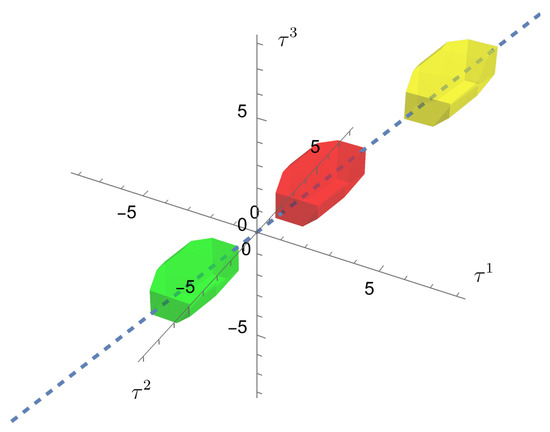
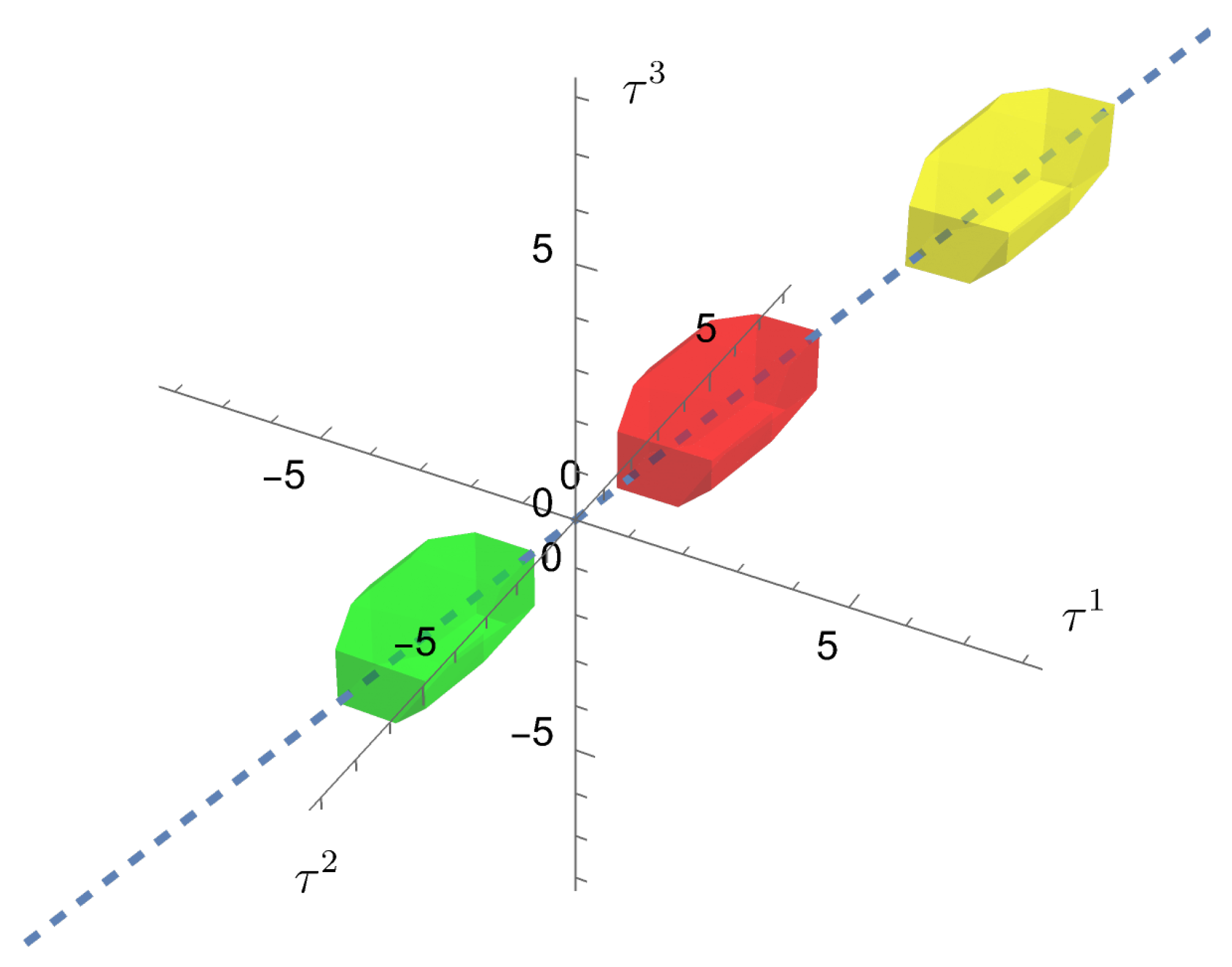
For different values of ${\tau }^4$, the shadow dodecahedron moves along the main bisectrix of the ${\mathcal{T}}_4$ grid without changing its shape (the relative positions of its vertices remain constant for every ${\tau }^4$). Figure 7 shows the shadow dodecahedron for $r_0=d=1$ and $\omega ={\displaystyle \frac{1}{2}}$$(\gamma ={\displaystyle \frac{2}{\sqrt{3}}})$ at ${\tau }^4=-2$, ${\tau }^4=2$ and ${\tau }^4=6$:

Figure 7. The shadow dodecahedron on the grid (${\mathcal{T}}_4$) for $r_0=d=1$ and $\omega ={\displaystyle \frac{1}{2}}$ at ${\tau }^4=-2$ (green), ${\tau }^4=2$ (red) and ${\tau }^4=6$ (yellow). The main bisectrix is also shown (dashed line).

5.4. Interpreting the RPS Solution

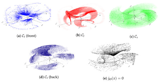
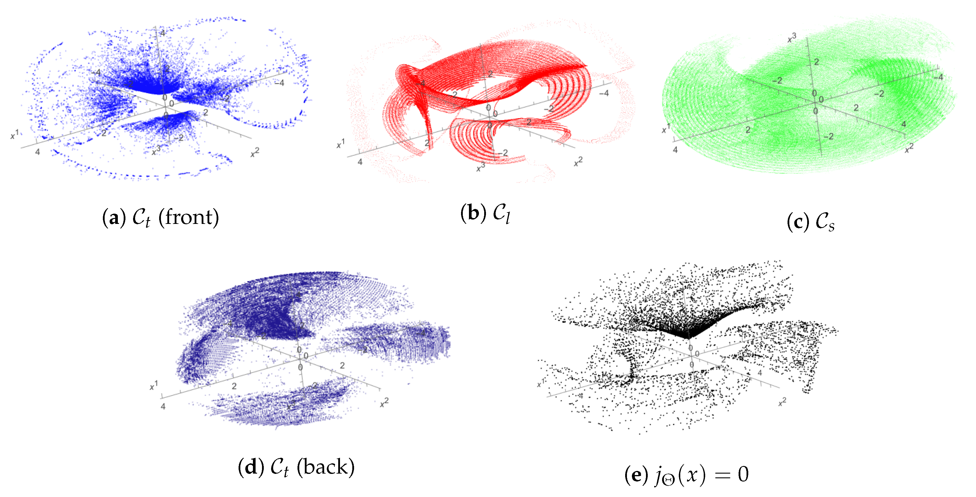
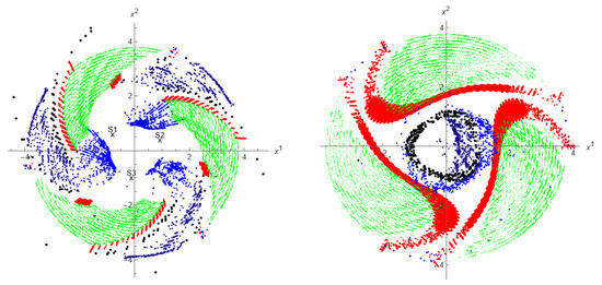
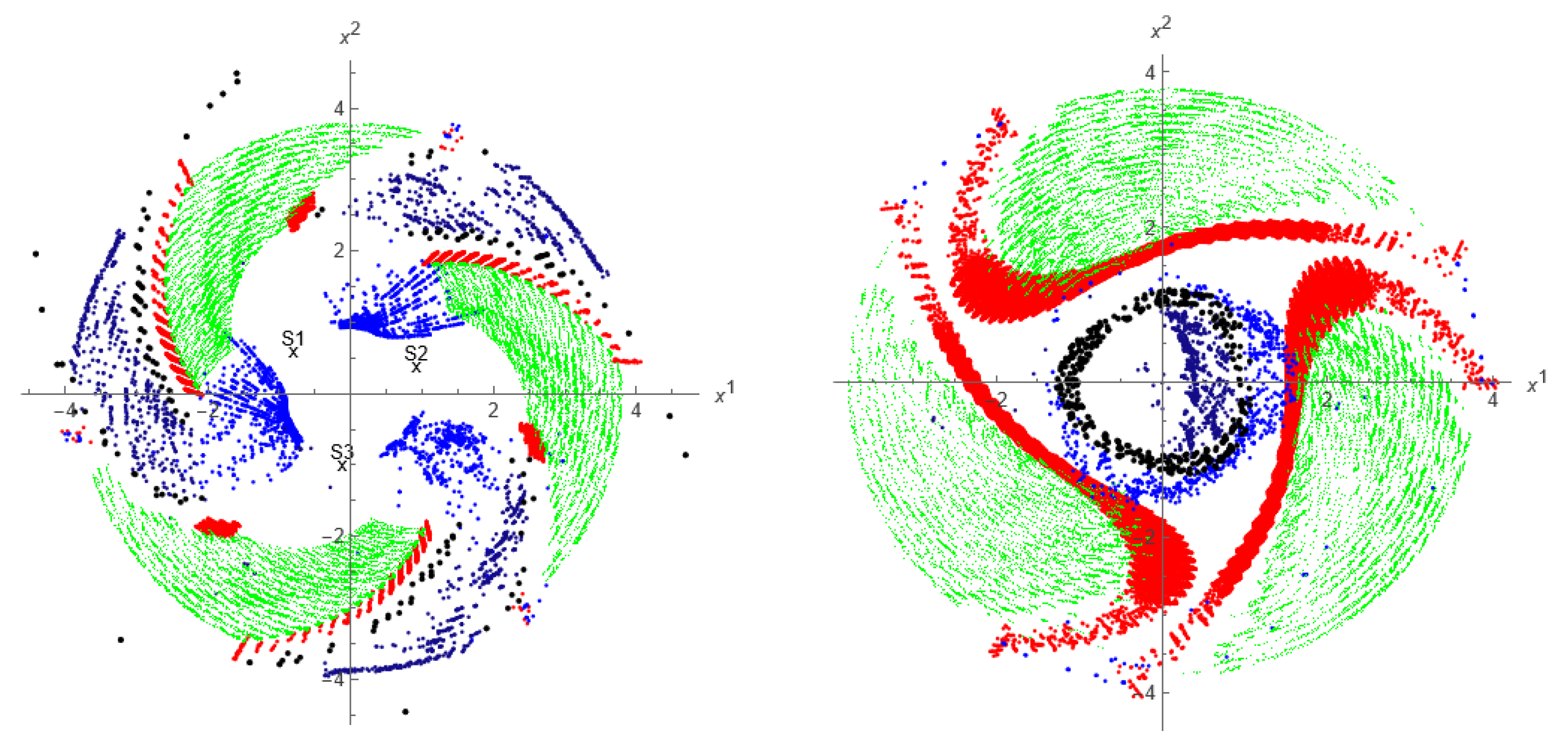
In this example, representing the characteristic regions of the RPS solution in Cartesian coordinates for a given inertial time is not straightforward. Since the null propagation Equation (2) cannot be solved analytically for ${\tau }^A$ (the characteristic emission function ($\mathrm{\Theta }$), i.e., ${\tau }^A={\mathrm{\Theta }}^A\left(x\right)$, cannot be obtained), we cannot directly express the configuration vector ($\chi$) in Cartesian coordinates for a given coordinate time ($x^0$). Instead, we proceed numerically, first classifying a sufficient number of quads of emission coordinates $\{{\tau }^1,{\tau }^2,{\tau }^3,{\tau }^4\}$ according to the configuration vector’s causal character associated with each of them. Then, we transform each of these quads to inertial coordinates using (5) and label the space-time points thus obtained with the same colour scheme as in previous examples. For each characteristic region, we compute a large number of points and select those with a given (common) inertial time ($x^0$). This process unavoidably leads to approximations, for which reason the following representations have to be considered qualitatively.12 Figure 8 illustrates these regions for $x^0=5$ ($r_0=d=1$ and $\omega ={\displaystyle \frac{1}{2}}$$(\gamma ={\displaystyle \frac{2}{\sqrt{3}}})$).

Figure 8. Illustration of the emission-configuration regions of an RPS (at $x^0=5$) with three uniformly rotating emitters and one static emitter for $r_0=d=1$ and $\omega ={\displaystyle \frac{1}{2}}$$(\gamma ={\displaystyle \frac{2}{\sqrt{3}}})$. Emission-configuration regions ${\mathcal{C}}_s$ (space-like), ${\mathcal{C}}_l$ (light-like) and ${\mathcal{C}}_t$ (time-like) are coloured in green, red and blue, respectively. The 3-surface where $j_{\mathrm{\Theta }}\left(x\right)$ vanishes is shown in black.

Figure 9 includes two two-dimensional slices of the emission-configuration regions illustrated in Figure 8: one through the plane expressed as $x^3=0$ containing emitters 1, 2 and 3 and the other through the plane expressed as $x^3=2$, both at $x^0=5$ with $r_0=d=1$ and $\omega ={\displaystyle \frac{1}{2}}$$(\gamma ={\displaystyle \frac{2}{\sqrt{3}}})$.

Figure 9. Slices of the emission-configuration regions shown in Figure 8 at $x^0=5$ with $r_0=d=1$ and $\omega ={\displaystyle \frac{1}{2}}$$(\gamma ={\displaystyle \frac{2}{\sqrt{3}}})$. The color convention is the same as in Figure 8. Left: slice through the plane expressed as $x^3=0$ containing emitters 1, 2 and 3. Crosses indicate approximate satellite positions. Right: slice through the plane expressed as $x^3=2$.

It is worth noting that there is a coverage gap due to the rotating motion of the coplanar satellites. This gap begins at the light-cylinder horizon, which, for a given coordinate time, forms at a certain spatial distance from the centre and extends to infinity. On the other hand, the gaps seen, for example, in Figure 9 (left) that lie inside the circular figure are artefacts of the numerical analysis.

To remark on the essential properties of the RPS solution in this example, we consider the inertial coordinate location of those users whose emission coordinates satisfy the restrictions of ${\tau }^1=\sigma$, ${\tau }^2=-\sigma ,{\tau }^3=-\sigma$ and ${\tau }^4=\gamma \sigma \equiv {\mathrm{\Gamma }}_4\left(\sigma \right)$. Using (34) and (1), we calculate the configuration vector as follows:

$$\begin{array}{c}{\chi }_{\mu }=\sqrt{3}{r}_0\left({\chi }_0,{\chi }_1,{\chi }_2,{\chi }_3\right),\end{array}$$

(42)

$$\begin{array}{c}\begin{array}{cccc}& {\chi }_0=-{\displaystyle \frac{d{r}_0}{2}}(1+2cos\left(2\omega {\mathrm{\Gamma }}_4\right)),\hfill & & {\chi }_1=2d{\mathrm{\Gamma }}_{4}cos\left(\omega {\mathrm{\Gamma }}_4\right),\hfill \\ & {\chi }_2=-2d{\mathrm{\Gamma }}_{4}sin\left(\omega {\mathrm{\Gamma }}_4\right),\hfill & & {\chi }_3=2r_0{\mathrm{\Gamma }}_{4}cos\left(2\omega {\mathrm{\Gamma }}_4\right).\hfill \end{array}\end{array}$$

(43)

To calculate the particular solution ($y_{*}$), the configuration bivector (H) is first computed using (34), (35), (8) and (7). Choosing the transversal vector ($\xi =u$), Equation (6) yields the following:

$$\begin{array}{c}{y}_{*\mu }={\displaystyle \frac{\sqrt{3}{r}_0}{D}}\left(0,y_{{*}_1},y_{{*}_2},y_{{*}_3}\right),D=-{\displaystyle \frac{\sqrt{3}}{2}}d{r}_0^2\left(1+2cos\left(2\omega {\mathrm{\Gamma }}_4\right)\right),\end{array}$$

(44)

$$\begin{array}{c}\begin{array}{cc}& y_{{*}_1}=-2d{\mathrm{\Gamma }}_4^{2}cos\left(\omega {\mathrm{\Gamma }}_4\right),y_{{*}_2}=2d{\mathrm{\Gamma }}_4^{2}sin\left(\omega {\mathrm{\Gamma }}_4\right),\hfill \\ & y_{{*}_3}={\displaystyle \frac{r_0}{4}}\left(d^2+r_0^2+2(d^2+r_0^2-4{\mathrm{\Gamma }}_4^2)cos\left(2\omega {\mathrm{\Gamma }}_4\right)\right).\hfill \end{array}\end{array}$$

(45)

With this choice of $\xi$, the transversality condition restricts this solution to

$$\{\sigma \in \mathbb{R}|\sigma \ne {\sigma }_t\equiv \pm {\displaystyle \frac{\pi }{\gamma \omega }}({\displaystyle \frac{1}{3}}+n),n\in {\mathbb{Z}}^{+}\}.$$

At $\sigma ={\sigma }_t$, emitters 1 and 3 are at the same spatial location $(-{\displaystyle \frac{1}{2}},{\displaystyle \frac{\sqrt{3}}{2}},0)$, leading to a degenerate situation. The solution (5) reads as follows:

$$\begin{array}{c}{x}^{\alpha }(\sigma ,-\sigma ,-\sigma ,\gamma \sigma )=(\gamma \sigma ,0,0,d)+y_{*}-{\displaystyle \frac{{\lambda }_1}{{\lambda }_2}}\chi ,\\ \begin{array}{cc}\hfill {\lambda }_1& ={\displaystyle \frac{3}{16}}{r}_0^2\left(64d^2{\mathrm{\Gamma }}_4^4+r_0^2{\left(2\left(d^2-4{\mathrm{\Gamma }}_4^2+r_0^2\right)cos\left(2\omega {\mathrm{\Gamma }}_4\right)+d^2+r_0^2\right)}^2\right),\hfill \\ \hfill {\lambda }_2& =D({\displaystyle \frac{3}{2}}{r}_0^4{\mathrm{\Gamma }}_{4}cos\left(2\omega {\mathrm{\Gamma }}_4\right)\left(2\left(d^2-4{\mathrm{\Gamma }}_4^2+r_0^2\right)cos\left(2\omega {\mathrm{\Gamma }}_4\right)+d^2+r_0^2\right)-12d^2{r}_0{\mathrm{\Gamma }}_4^3+\widehat{ϵ}D\sqrt{{\mathrm{\Delta }}_{\sigma }}),\hfill \\ \hfill {\mathrm{\Delta }}_{\sigma }& ={\lambda }_1-3r_0^2{\mathrm{\Gamma }}_4^2(d^2+r_0^2).\hfill \end{array}\end{array}$$

(46)

In this case, the emission-reception conditions (3) are expressed as follows:

$$|{\mathrm{\Gamma }}_4|<{\displaystyle \frac{1}{2}}{r}_0\sqrt{2(1+sin(\pm 2\omega {\mathrm{\Gamma }}_4+{\displaystyle \frac{\pi }{6}})},\left|{\mathrm{\Gamma }}_4\right|<{\displaystyle \frac{1}{2}}\sqrt{r_0^2+d^2}.$$

(47)

Table 3 shows the result of setting $r_0=d=1$ and $\omega ={\displaystyle \frac{1}{2}}$$(\gamma ={\displaystyle \frac{2}{\sqrt{3}}})$ for different values of $\sigma$. In this particular case, the previous emission-reception conditions impose $-{\sigma }_c<\sigma <{\sigma }_c$, with ${\sigma }_c\approx 0.570$. However, unlike in previous examples, the “physical” requirement of ${\mathrm{\Delta }}_{\sigma }\ge 0$ further restricts the domain to $-{\sigma }_p\le \sigma \le {\sigma }_p$, with ${\sigma }_p\approx 0.453$ in this case.

Table 3. RPS solution with $r_0=d=1$ and $\omega ={\displaystyle \frac{1}{2}}$$(\gamma ={\displaystyle \frac{2}{\sqrt{3}}})$ for users with ${\tau }^1=\sigma$,${\tau }^2=-\sigma ,{\tau }^3=-\sigma$ and ${\tau }^4=\gamma \sigma$.

$\mathit{\sigma }$	${\mathit{\chi }}^2$	${\mathbf{\Delta }}_{\mathit{\sigma }}$	${\mathit{x}}^0$	$({\mathit{x}}^1,{\mathit{x}}^2,{\mathit{x}}^3)$	Emission Solutions
$-{\displaystyle \frac{2}{5}}$	<0	>0	≈2.654	≈$(-1.710,-0.402,-1.573)$	$\widehat{ϵ}=-1$ One emission solution
≈0.447	0	>0	≈3.764	≈$(2.746,-0.726,2.470)$	$\widehat{ϵ}=-1$ One emission solution
≈0.450	>0	>0	≈20.506	≈$(15.055,-4.002,13.522)$	$\widehat{ϵ}=1$
			≈2.992	≈$(2.197,-0.584,1.973)$	$\widehat{ϵ}=-1$
					Two emission solutions

(i)

For $\sigma =-{\displaystyle \frac{2}{5}}$, the emitter configuration is space-like at

$x^{\alpha }\approx \left(2.654,-1.710,-0.402,-1.573\right)$, which is the sole emission solution (with $\widehat{ϵ}=-1$). The solution with $\widehat{ϵ}=1$ is a reception solution.

(ii)

For $\sigma \approx 0.447$, the emitter configuration is light-like at

$x^{\alpha }\approx \left(3.764,2.746,-0.726,2.470\right)$, which is the sole emission solution (with $\widehat{ϵ}=-1$). The solution with $\widehat{ϵ}=1$ is degenerate.

(iii)

For $\sigma \approx 0.450$, the emitter configuration is time-like at

$x_{+}^{\alpha }\approx (20.506,15.055,-4.002,13.522)$ and

$x_{-}^{\alpha }\approx (2.992,2.197,-0.584,1.973)$, both being emission solutions (with $\widehat{ϵ}=1$ and $\widehat{ϵ}=-1$, respectively); $x_{-}\left(x_{+}\right)$ is in the front (back) emission coordinate domain.

6. Summary and Conclusions

A basic construction of an RPS involving four static emitters in flat space-time was presented in [9]. The same procedure has been extended in the present work by including inertial, accelerated and rotating emitters. All these constructions provide clarifying examples of the notions involved in RPS theory (null propagation equations; bifurcation of solutions; grid space of emission coordinates; emission/reception conditions; shadows reciprocally cast by pairs of emitters; shadow dodecahedrons; emission coordinate regions; central, front, and back regions; orientation; etc.). Although the solution for the location problem in RPS theory has been extensively analysed in an abstract setting for Minkowski space-time [10,11,12], there are no studies involving non-trivial examples of RPSs. This article intends to fill that gap.

The shadow dodecahedron is the representation in a 3-grid of the volume enclosed by the six inequalities of the emission/reception conditions. These inequalities involve absolute values; therefore, each of them defines two 2-planes, yielding a dodecahedron. From the study of the shadow dodecahedron of the rotating example (Section 5.3), we conclude that the specific intersection of these planes is what determines the number of vertices. If we were to consider $k>4$ satellites, each of the dodecahedra would correspond to groups of four satellites, three of which would not change—only the fourth one. In this way, this union of dodecahedra may be represented in the same 3-grid. In general, configurations formed with $k\ge 4$ satellites can be studied (in different grids) based on the $\left({\displaystyle \genfrac{}{}{0pt}{}{k}{4}}\right)$ combinations of the corresponding shadow dodecahedra.

The analysed examples offer a method to explore more involved constructions in flat and curved space-times. It may be productive to study and classify types of motions according to the vertices of the dodecahedra. Given a time-like vector field (informing us about a certain kinematic or gravitational property in a known space-time), it makes sense to take four of its integral curves as emitter world lines of a RPS—in particular, four static observers in Schwarzchild space-time or four geodesic ones in radial motion. A numerical approach to obtain the emission coordinates in this last case was presented in [24]. A situation that we plan to consider in future work is that of four emitters in conformal radial motion. The world lines of such emitters are the integral curves of a radial conformal Killing field in flat space-time [25,26]. In particular, we could study the expanding radial case (Milne Universe [27,28]) to mimic an RPS in Cosmology with galactic emitters co-moving with matter, as modelled in Friedmann–Lemaître–Robertson–Walker geometry.

Furthermore, our incipient constructions of the emission-coordinate regions attached to a specific RPS can be complemented with additional theoretical information, such as the IDEAL (Intrinsic, Deductive, Explicit, Algorithmic) characterization of gravitational fields developed in [29,30,31,32], which is necessary in order to do gravimetry (determining the true gravitational potentials) in an unknown space-time region (see [6] for details concerning this idea, [33] for application of optimization methods in GNSS to obtain space-time metric information from parametrized models and [34] for general considerations on relativistic gravimetry and its current status).

The examples analysed in this article are basic constructions from which to extract valuable information before considering more complicated settings. This analysis may play a crucial role in RPS theory, similar to the one played in plant biology by model organism Arabidopsis thaliana. The study of this model plant, which—as far as we know—has little practical application in agriculture, has paved the way towards our understanding of more complex plants. Similarly, the RPS constructions considered here may, in principle, lack practical significance; nevertheless, they contain valuable information for the development of RPSs in a (known or unknown) gravitational field geometry.

References

- Coll, B.; Pozo, J.M. Relativistic positioning systems: The emission coordinates. Class. Quantum Gravity 2006, 23, 7395. [Google Scholar] [CrossRef] [Scilit]
- Coll, B.; Ferrando, J.J.; Morales-Lladosa, J.A. Newtonian and relativistic emission coordinates. Phys. Rev. D 2009, 80, 064038. [Google Scholar] [CrossRef] [Scilit]
- Synge, J. Relativity: The General Theory; North-Holland: Amsterdam, The Netherlands, 1960. [Google Scholar]
- Bahder, T.B. Navigation in curved space-time. Am. J. Phys. 2001, 69, 315–321. [Google Scholar] [CrossRef] [Scilit]
- Blumenthal, L.M. Theory and Applications of Distance Geometry, 2nd ed.; Chelsea Publishing Company: New York, NY, USA, 1970. [Google Scholar]
- Coll, B. Epistemic Relativity: An Experimental Approach to Physics; Springer International Publishing: Berlin/Heidelberg, Germany, 2019; pp. 291–315. [Google Scholar] [CrossRef] [Scilit]
- Coll, B. Elements for a Theory of Relativistic Coordinate Systems: Formal and Physical Aspects; World Scientific: Singapore, 2001; pp. 53–65. [Google Scholar] [CrossRef] [Scilit]
- Coll, B. Relativistic positioning systems: Perspectives and prospects. Acta Futur. 2013, 7, 35–47. [Google Scholar] [CrossRef] [Scilit]
- Serrano Montesinos, R.; Morales-Lladosa, J.A. Minkowskian Approach to the Pseudorange Navigation Equations. Universe 2024, 10, 179. [Google Scholar] [CrossRef] [Scilit]
- Coll, B.; Ferrando, J.J.; Morales-Lladosa, J.A. Positioning systems in Minkowski spacetime: From emission to inertial coordinates. Class. Quantum Gravity 2010, 27, 065013. [Google Scholar] [CrossRef] [Scilit]
- Coll, B.; Ferrando, J.J.; Morales-Lladosa, J.A. Positioning systems in Minkowski space-time: Bifurcation problem and observational data. Phys. Rev. D 2012, 86, 084036. [Google Scholar] [CrossRef] [Scilit]
- Serrano Montesinos, R.; Ferrando, J.J.; Morales-Lladosa, J.A. Location Problem in Relativistic Positioning: Relative Formulation. Universe 2024, 10, 299. [Google Scholar] [CrossRef] [Scilit]
- Delva, P.; Kostić, U.; Čadež, A. Numerical modeling of a Global Navigation Satellite System in a general relativistic framework. Adv. Space Res. 2011, 47, 370–379. [Google Scholar] [CrossRef] [Scilit]
- Kostić, U.; Horvat, M.; Gomboc, A. Relativistic Positioning System in perturbed spacetime. Class. Quantum Gravity 2015, 32, 215004. [Google Scholar] [CrossRef] [Scilit]
- Puchades, N.; Sáez, D. Approaches to relativistic positioning around Earth and error estimations. Adv. Space Res. 2016, 57, 499–508. [Google Scholar] [CrossRef] [Scilit]
- Carloni, S.; Fatibene, L.; Ferraris, M.; McLenaghan, R.G.; Pinto, P. Discrete relativistic positioning systems. Gen. Relativ. Gravit. 2020, 52, 12. [Google Scholar] [CrossRef] [Scilit]
- Feng, J.C.; Hejda, F.; Carloni, S. Relativistic location algorithm in curved spacetime. Phys. Rev. D 2022, 106, 044034. [Google Scholar] [CrossRef] [Scilit]
- Coll, B.; Ferrando, J.J.; Morales, J.A. Two-dimensional approach to relativistic positioning systems. Phys. Rev. D 2006, 73, 084017. [Google Scholar] [CrossRef] [Scilit]
- Coll, B.; Ferrando, J.J.; Morales, J.A. Positioning with stationary emitters in a two-dimensional space-time. Phys. Rev. D 2006, 74, 104003. [Google Scholar] [CrossRef] [Scilit]
- Coll, B.; Ferrando, J.J.; Morales-Lladosa, J.A. Positioning in a flat two-dimensional space-time: The delay master equation. Phys. Rev. D 2010, 82, 084038. [Google Scholar] [CrossRef] [Scilit]
- Pozo, J. Constructions in 3D (I) and (II); Talks delivered at the School on Relativistic Coordinates, Reference and Positioning Systems; University of Salamanca: Salamanca, Spain, 2005. [Google Scholar]
- Compagnoni, M.; Notari, R.; Antonacci, F.; Sarti, A. A comprehensive analysis of the geometry of TDOA maps in localization problems. Inverse Probl. 2014, 30, 035004. [Google Scholar] [CrossRef] [Scilit]
- Compagnoni, M.; Notari, R.; Antonacci, F.; Sarti, A. On the statistical model of source localization based on Range Difference measurements. J. Frankl. Inst. 2017, 354, 7183–7214. [Google Scholar] [CrossRef] [Scilit]
- Bunandar, D.; Caveny, S.A.; Matzner, R.A. Measuring emission coordinates in a pulsar-based relativistic positioning system. Phys. Rev. D 2011, 84, 104005. [Google Scholar] [CrossRef] [Scilit]
- Herrero, A.; Morales, J.A. Radial conformal motions in Minkowski space-time. J. Math. Phys. 1999, 40, 3499–3515. [Google Scholar] [CrossRef] [Scilit]
- De Lorenzo, T.; Perez, A. Light cone thermodynamics. Phys. Rev. D 2018, 97, 044052. [Google Scholar] [CrossRef] [Scilit]
- Synge, J.L. Relativity: The Special Theory; North-Holland Publishing Company; Interscience Publishers: Amsterdam, The Netherlands; New York, NY, USA, 1956. [Google Scholar]
- Rindler, W. Essential Relativity; Special, General, and Cosmological; Van Nostrand Reinhold Co.: New York, NY, USA, 1969. [Google Scholar]
- Ferrando, J.J.; Sáez, J.A. An intrinsic characterization of the Schwarzschild metric. Class. Quantum Gravity 1998, 15, 1323. [Google Scholar] [CrossRef] [Scilit]
- Ferrando, J.J.; Sáez, J.A. An intrinsic characterization of the Kerr metric. Class. Quantum Gravity 2009, 26, 075013. [Google Scholar] [CrossRef] [Scilit]
- Ferrando, J.J.; Sáez, J.A. An intrinsic characterization of spherically symmetric spacetimes. Class. Quantum Gravity 2010, 27, 205024. [Google Scholar] [CrossRef] [Scilit]
- Mengual, S. Physical interpretation of spherically symmetric perfect fluid solutions to Einstein’s equations. arXiv 2026, arXiv:2512.19212. [Google Scholar]
- Tarantola, A.; Klimes, L.; Pozo, J.M.; Coll, B. Gravimetry, Relativity, and the Global Navigation Satellite Systems. arXiv 2009, arXiv:0905.3798. [Google Scholar] [CrossRef] [Scilit]
- Delva, P.; Geršl, J. Theoretical Tools for Relativistic Gravimetry, Gradiometry and Chronometric Geodesy and Application to a Parameterized Post-Newtonian Metric. Universe 2017, 3, 24. [Google Scholar] [CrossRef] [Scilit]
Disclaimer/Publisher’s Note: The statements, opinions and data contained in all publications are solely those of the individual author(s) and contributor(s) and not of MDPI and/or the editor(s). MDPI and/or the editor(s) disclaim responsibility for any injury to people or property resulting from any ideas, methods, instructions or products referred to in the content. |
© 2026 by the authors. Licensee MDPI, Basel, Switzerland. This article is an open access article distributed under the terms and conditions of the Creative Commons Attribution (CC BY) license.