GCSNet: A Multi-Modal Fusion Network with Cosine Similarity for Galaxy Classification

Abstract

Galaxy classification is essential for understanding the formation and evolution of cosmic structures. However, faced with the explosive growth of astronomical observation data, traditional single-modality classification methods relying solely on spectroscopy or imaging have struggled to meet high-precision demands due to insufficient feature utilization and limited generalization capability. Therefore, multimodal fusion has emerged as a promising direction by leveraging information complementarity to overcome the limitations of single data sources. Accordingly, this paper proposes a model named Galaxy CosineNet (GCSNet), which integrates imaging, spectroscopic, and tabular data for high-precision galaxy classification. Specifically, the model employs dedicated encoders to process the three modalities separately and utilizes skip connections to preserve raw features. Furthermore, it incorporates a multi-head self-attention mechanism to deeply mine global cross-modal complementary information. Finally, these features are concatenated and fed into a cosine similarity classification head. Experimental results demonstrate that GCSNet achieves 97.15% accuracy in classifying star-forming, composite, active galactic nuclei (AGNs), and normal galaxies. This performance outperforms the best single-modal baseline, GaSNet, by 0.76% and mainstream multi-modal models such as MB-ISTL and the Transformer by over 1.6%. Consequently, the proposed GCSNet offers an effective and novel approach for research on automatic galaxy classification.

1. Introduction

Since Hubble [1] (1926) proposed the morphological sequence, the study of galaxy classification has undergone a century of development, transitioning from traditional visual inspection to modern deep learning. Current classification systems primarily rely on two complementary approaches: morphological classification, which categorizes galaxies (e.g., ellipticals, spirals, and irregulars) based on geometric appearance; and physical classification, which utilizes spectral characteristics to distinguish physical states, such as star-forming galaxies, active galactic nuclei (AGNs), and their subclasses. These two systems are complementary, jointly form the cornerstone of modern galaxy research, advancing the exploration of distant galaxies.

In the realm of morphological classification, the field has shifted from traditional machine learning to deep learning. Early works, such as Odewahn et al. [2] (1992), pioneered the use of neural networks combined with photometric parameters to achieve automatic separation of stars from galaxies. With the advent of deep learning, convolutional neural networks (CNNs) became mainstream. For instance, Dai [3] (2018) applied an improved ResNet architecture to the Galaxy Zoo dataset for five galaxy morphologies (circular, intermediate, cigar-shaped, edge-on, and spiral), surpassing classical methods. Subsequently, Yang et al. [4] (2021) achieved 98.23% accuracy in a star-galaxy binary classification task. More recently, Kong et al. [5] (2024) further improved performance by introducing a channel attention mechanism for five-class galaxy classification, reaching an accuracy of 99.37%. However, as classification accuracy approaches its ceiling, the research focus has begun to shift. Wu & Walmsley [6] (2025) moved beyond merely improving accuracy to explore interpretable representation learning methods. By introducing Sparse Autoencoders (SAE) to the Euclid Q1 survey data, they extracted features with clear physical meanings from the feature space of pre-trained neural networks. This approach not only successfully reproduced the known morphological classifications predefined by Galaxy Zoo but also discovered new features previously undefined by humans (such as dust lanes in edge-on disk galaxies and elliptical galaxies with blue companions). This demonstrates that, driven by deep learning, galaxy morphology research is advancing toward higher-dimensional interpretability and automation. It is worth noting that despite the simultaneous improvement in image classification accuracy and interpretability, methods relying solely on the image modality often struggle to capture the complex physical processes within galaxies, posing a risk of misjudgment when facing celestial objects with similar morphology but distinct physical properties.

In the realm of spectral-based physical classification, Baldwin et al. [7] (1981) proposed the optical diagnostic map BPT for emission-line galaxies. Connolly et al. [8] (1995) utilized PCA in early works to demonstrate the physical correlation between continuous spectral variations and morphological sequences. Subsequently, deep learning methods were introduced into spectral classification to improve classification accuracy by utilizing spectral physical information. Wu et al. [9] (2023) developed GalSpecNet, a 1D CNN model using emission-line features to classify star-forming, composite, AGN, and normal galaxies. It achieved over 93% accuracy, with visualizations showing consistency with traditional BPT diagnostic lines. Later, Zhong et al. [10] (2024) further proposed the GasNet-II architecture. It reached 96% accuracy in star/galaxy/quasar classification and performed simultaneous redshift prediction. Although spectral data is rich in physical information, it is limited by the coverage range of optical fibers and the scarcity of labeled samples, making it difficult to meet the requirements of all-sky classification of large-scale surveys when used alone.

In light of the inherent limitations of a single modality, exploring the deep physical connection between images and spectra has become an inevitable trend. In recent years, studies have confirmed the feasibility of inferring galaxy spectral features and physical states from images, providing a new pathway to overcome the high cost and limited coverage of spectroscopic data. Wu & Boada [11] (2019) pioneered the use of a deep residual CNN to successfully predict galaxy gas-phase metallicity using only SDSS gri three-band images. With 128 × 128 pixel image inputs, the root mean square error (RMSE) between the predicted and true values was only 0.085 dex, significantly outperforming a traditional random forest algorithm on the same dataset (RMSE = 0.130 dex). This result fully revealed the rich chemical information embedded in photometric images. Wu & Peek [12] (2020) advanced this line of research by pioneering the robust prediction of galaxy spectra directly from broadband images. Their hybrid CNN architecture successfully reconstructed full spectra from images, capturing critical emission-line features. Notably, the BPT classifications derived from these predicted spectra demonstrated strong generalizability even for objects outside the training distribution, such as the peculiar Rubin galaxies. This finding preliminary validated the model’s extrapolation capability, a finding subsequently corroborated by Holwerda et al. [13] (2021). Alfonzo et al. [14] (2024) proposed the interpretable CNN framework Katachi, which pushed this line of thinking to a deeper level. Their model not only predicts current star formation rates from images but also reconstructs the complete past star formation history of galaxies (e.g., half-mass time). Furthermore, using the SHAP method, it revealed how different morphological features, such as bulges and spiral arms, encode physical processes on different timescales.

Although image-based prediction can indirectly infer physical states, it cannot fully replace the direct diagnosis of spectroscopy. Therefore, to truly break through the classification bottleneck, it is necessary to deeply integrate morphological structure with spectral information, making multi-modal fusion an inevitable path. Wei et al. [15] (2023) proposed the BATMM model, which incorporates the Transformer self-attention mechanism, combining image and spectral data to identify blue horizontal branch stars. The results were higher than the accuracy achieved by any single modality, effectively validating the potential of multi-modal fusion. Deng et al. [16] (2024) proposed the multimodal ensemble model MESCR, achieving 96.1% accuracy in the five-class classification of A-, F-, G-, K-, and M-type stars, and constructed a predictive catalog containing over 50 million stars. These studies fully demonstrate that effectively integrating heterogeneous data can significantly enhance the generalization ability and physical interpretability of models. In the same year, Rizhko & Bloom [17] constructed a multimodal dataset comprising time-series photometry, spectra, and metadata. By leveraging the complementarity of these three modalities to classify ten types of variable stars, their model achieved an accuracy of 94.07%, offering a new perspective on multi-source astronomical data fusion. Junell et al. [18] (2025) leveraged a hybrid architecture of encoders and CNNs on four modalities (photometry, image cutouts, metadata, and spectra) to realize a unified framework for the automatic classification of transients and variables.

Although considerable progress has been made in multimodal galaxy classification, significant challenges remain in the fine-grained classification of four types of galaxies with distinct physical mechanisms: star-forming galaxies, composite galaxies, active galactic nuclei (AGNs), and normal galaxies. These four types of galaxies differ fundamentally in their physical nature: star-forming galaxies [19] are dominated by young massive stars and exhibit distinct spiral arms and bluer ultraviolet radiation; composite galaxies [20] feature both star formation and weak AGN activity, with spectral characteristics in a transitional state; AGNs [21] are powered by central black hole accretion and have extremely compact nuclear regions; and normal galaxies [22] lack prominent ionization sources, presenting reddened, smooth morphological structures and weak spectral emission lines. Together, they form a complete galaxy evolution sequence ranging from intense star formation activity to quiescent evolutionary states. Affected by dust extinction, redshift effects, spatial resolution, and other factors, these four types of galaxies exhibit strong degeneracy in the optical color space, making effective differentiation difficult using traditional photometric methods alone [20]. In spectral physical analysis, the emission-line ratios of composite galaxies and low-signal-to-noise AGNs easily fall into the ambiguous boundary region of the BPT diagram, making them highly prone to confusion due to overlapping ionization mechanisms [23]. Although various single-modal and multi-modal methods have been proposed for galaxy classification, the fine-grained classification of the above four types of galaxies with distinct physical mechanisms still faces the following two core challenges. The first challenge is the limitation of feature representation. Most current models simply concatenate or perform weighted summation of the features of images and spectra when processing them. This shallow fusion approach struggles to capture deep cross-modal correlations. More importantly, these models often overlook key global physical parameters such as redshift and signal-to-noise ratio, leaving them unable to perceive cosmological distances or assess data quality. This leads to confusion between galaxies with similar redshifts but different physical types. The second challenge is the bottleneck of model architecture. Traditional direct concatenation or weighted fusion mechanisms tend to lose shallow spatial and morphological information during layer-by-layer feature extraction. Moreover, when faced with class imbalance (e.g., scarce AGNs versus abundant star-forming galaxies), classification boundaries become biased, resulting in misclassification of transitional types such as composite galaxies. To address these challenges, we propose a multi-modal galaxy classification algorithm named GCSNet, designed for fine-grained physical classification. The model innovates in three dimensions (new modality introduction, feature interaction, and decision mechanism) to address insufficient single-modal representation, inadequate cross-modal interaction, and class imbalance. The main contributions are as follows.

(1)

To address the limitation of feature representation, we introduce tabular data as a third modality to complement photometric imaging and spectroscopic information. The selected tabular data consist of four parameters: spectroscopic redshift (z), median spectral signal-to-noise ratio (Median SNR), Galactic extinction E(B − V), and $H\alpha$ equivalent width ($EW\_H\alpha \_6562$). Here, redshift reflects the distance of the galaxy; the signal-to-noise ratio characterizes the overall quality of the spectral data; E(B − V) represents the extinction level of the Galactic foreground dust; and the equivalent width reflects the radiation strength of ionized gas, which is closely related to the star formation rate. By leveraging this global physical information, the model can more easily distinguish galaxies with different ionization mechanisms, such as star-forming galaxies and AGNs.

(2)

To avoid losing original features during the fusion process, this paper employs skip connections to directly transmit shallow information to deeper layers. At the same time, a multi-head self-attention mechanism is introduced to enable the model to automatically learn the correlations among images, spectra, and tabular data. Finally, the original features and the fused features are concatenated together for the final classification.

(3)

To address the issue of class imbalance, we introduce class weights in the loss function as a mitigation strategy. In addition, we propose a classification decision head based on cosine similarity [24]. By leveraging its property of focusing on feature direction rather than magnitude, it avoids interference caused by variations in feature magnitude, further improving the stability and accuracy of classification.

Experiments on the Sloan Digital Sky Survey Data Release 17 (SDSS DR17) dataset demonstrate that the model achieves an overall accuracy of 97.15%. Furthermore, in the classification of composite galaxies with similar physical morphologies, it outperforms the GasNet model by 5.18%, exhibiting superior robustness.

The structure of this paper is organized as follows: Section 2 describes the dataset, data preprocessing techniques; Section 3 elaborates on the network architecture of GCSNet; Section 4 presents and discusses the experimental results and ablation analysis; finally, Section 5 summarizes the main conclusions of the paper.

2. Data and Preprocessing

2.1. Dataset Construction

The data in this paper are derived from SDSS DR17 [25]. Through the CasJobs interface, we integrated image morphological, spectral physical, and tabular statistical features to construct a multimodal dataset containing 68,917 high-quality galaxies. The sample consists of 33,291 star-forming galaxies, 13,131 composite galaxies, 7662 AGNs, and 14,833 normal galaxies. Given that Seyfert galaxies and low-ionization nuclear emission-line region galaxies (LINERs) exhibit similar spectral characteristics and are relatively scarce (5636 and 2026, respectively), we merged them into a single AGNs category to optimize class distribution balance.

To ensure the physical reliability and classification validity of the data, we adhere to the following rigorous sample screening and data construction pipeline.

2.1.1. Sample Screening and Quality Control

Galaxy subclass selection. Star-forming galaxies, composite galaxies, and AGNs are easily confused due to their overlapping ionization mechanisms and thus need to be clearly distinguished. In contrast, normal galaxies, though silent in terms of emission lines, represent an indispensable endpoint in the evolutionary sequence.

Star and contaminant removal. Stars appear as point sources in SDSS images [26], morphologically distinct from galaxies, which are extended sources. If stars were included in the classification task, the model could easily achieve high accuracy by distinguishing point-like from extended sources. This would distract its learning capacity from capturing the subtle physical differences among star-forming galaxies, composites, AGNs, and normal galaxies. Therefore, we remove stars and quasars as contaminants using the SDSS official class = ‘GALAXY’ label, retaining only galaxy samples.

Redshift quality control. To ensure the physical integrity of the spectral data, we restrict the spectroscopic redshift range to 0 < z < 0.3 and retain only samples with the redshift quality flag Zwarning = 0 to guarantee the reliability of the redshift measurements. This range ensures that key BPT diagnostic lines such as $H\alpha 6563$, $\left[\mathrm{NII}\right]6584$, $\left[\mathrm{OIII}\right]5007$, $H\beta 4861$ fall fully within the SDSS spectral coverage area (3800 Å–9200 Å) [27].

Tabular parameter selection. We introduce four key parameters to complement the global information from four dimensions: distance, data quality, observing environment, and ionization strength. Spectroscopic redshift (z) reflects the cosmological distance of galaxies, helping the model distinguish the evolutionary stages of galaxies at different redshifts [28]. The median spectral signal-to-noise ratio (snMedian) [29] characterizes the overall quality of the spectral data. We require snMedian > 10 to ensure that the weak spectral features of each galaxy type, especially the faint emission lines of normal galaxies and the ambiguous boundaries of composite galaxies, can be reliably observed. Galactic extinction E(B − V) [30] quantifies the effect of Milky Way foreground dust on observed colors, serving as an observational prior to help the model disentangle Galactic reddening from intrinsic galaxy colors. The $H\alpha$ equivalent width ($EW\_H\alpha \_6562$) [31] is directly linked to the star formation rate, reflecting the radiation strength of ionized gas, and serves as a key indicator for distinguishing star-forming galaxies from AGNs. Together, these four parameters provide independent and complementary physical priors to the imaging and spectral modalities, addressing distance scale, data reliability, environmental interference, and ionization mechanisms.

2.1.2. Multi-Modal Data Preparation

Data access and acquisition. Through the SDSS official CasJobs platform, we executed SQL queries on the DR17 database, joining the photoobj (photometry table), specobj (spectroscopy table), and emissionLinesPort (emission-line parameter extension table). Using the unique identifier ObjID of each astronomical object in the database as the join key, we ensured that every sample simultaneously possesses photometric, spectroscopic, and emission-line diagnostic information [9].

Image modality. We select u, g, r three-band images sensitive to the physical state of galaxies. Specifically, the u band reveals AGN features, the g band traces star-forming regions, and the r band reflects stellar mass distribution [32].

Spectral modality. Using celestial coordinates (RA/DEC), we match imaging and spectroscopic data from different SDSS tables to construct paired samples required for multi-modal learning. The coordinates are used only for alignment and are not input as classification features. After matching, the spectrum of each galaxy is paired with its corresponding three-channel false-color image to form multi-modal data pairs for subsequent model training.

Tabular modality. The four tabular parameters obtained through the SQL queries described above, namely spectroscopic redshift (z), median spectral signal-to-noise ratio (snMedian), Galactic extinction E(B − V), and $H\alpha$ equivalent width ($EW\_H\alpha \_6562$), have their specific physical meanings and roles in classification detailed in the sample screening section.

The entire dataset is randomly divided into a training set, a validation set, and a test set with a ratio of 70%, 15%, and 15%, respectively, and the detailed sample distribution is shown in Table 1. The basic data of this paper can be obtained from SDSS, with the URL: https://dr17.sdss.org/ (catalog data) (accessed on 16 April 2026).

Table 1. The distribution of galaxy subclasses in the dataset.

Class	Train Set	Valid Set	Test Set	Total
Star Forming	23,303	4994	4994	33,291
Composite	9191	1970	1970	13,131
AGN	5364	1149	1149	7662
Normal	10,383	2225	2225	14,833
Total	48,241	10,338	10,338	68,917

2.2. Data Preprocessing

2.2.1. Image Data Preprocessing

The photometric images used in this paper were sourced from the SDSS Science Archive Server (SAS) as part of SDSS Data Release 17 (DR17) and stored in FITS format [33] with three independent bands of u, g, and r. It should be explicitly noted that these images are SDSS corrected frames (fpC files), which have been processed by the official SDSS pipeline to remove instrumental signatures (including bias, dark, and flat-fielding) and calibrated to nanomaggies. They are exactly the same images used by the SDSS photometric pipeline to generate the PhotoObjAll catalog. They are neither raw unprocessed images nor coadded images from multiple exposures. During image downloading, the program reads parameters such as RA, Dec, run, camcol, and field from the CSV file. Combined with the world coordinate system (WCS) embedded in the FITS headers, it locates the target astronomical object from the corrected frames and extracts a 300 × 300 pixel subimage centered on the galaxy. This strategy ensures target uniqueness, significantly reduces data volume, and preserves the original photometric accuracy of the FITS format. Due to the field-of-view differences among different bands, direct synthesis can lead to spatial misalignment and distortions in physical information. To address this, we employed the standardized RGB Synthesis program developed by He et al. [34] for multi-band registration. The program uses the r-band image as the reference coordinate system and strictly aligns the u- and g-band images through geometric transformations. A center crop is then performed based on the minimum common width and height to ensure pixel-level spatial consistency. After alignment, the registered u, g, and r single-band images are synthesized into a three-channel false-color image, which is used to learn the morphological structural features of galaxies (e.g., spiral arms, bulges, dust lanes). Finally, to eliminate differences in the distribution and numerical range of gray values among images of different bands, Z-score normalization is performed independently on each channel of each image. The normalization is defined as shown in Equation (1):

$$x’={\displaystyle \frac{x-\mu }{\sigma }}$$

(1)

where $x$ represents the original pixel value, $\mu$ and $\sigma$ denote the mean and standard deviation of the specific band, respectively. Although per-channel Z-score normalization alters the absolute color ratios of galaxies, it preserves the spatial structure, morphological texture, brightness distribution, and inter-band morphological differences within each band. Through this preprocessing pipeline, we constructed multi-band image inputs that are spatially aligned, uniform in resolution, and statistically normalized, ready for subsequent model training.

2.2.2. Spectral Data Preprocessing

The SDSS DR17 original spectrum covers approximately 3800 Å–9200 Å, with a total of 3843 sampling points, mainly consisting of continuous spectra, absorption/emission lines, and noise [35]. As previous studies have pointed out, considering that the SDSS spectra have not undergone absolute flux calibration, the absolute intensity of the continuous spectra is unreliable, while the relative intensity ratios of emission lines (such as $\left[\mathrm{OIII}\right]/\mathrm{H}\mathsf{\beta }$, $\left[\mathrm{NII}\right]/\mathrm{H}\mathsf{\alpha }$) are the key basis for physical classification [36]. Directly inputting original fluxes not only introduces dimensional differences but is also vulnerable to baseline drift and noise interference. Therefore, we have constructed two spectral input strategies to explore the impact of different feature representations on classification performance:

(1)

Observed Spectra and Robust Normalization

First, we extracted the traffic data from the COADD extension table of the FITS file, replacing non-numeric values (NaN) with zeros and discarding invalid samples with a standard deviation below 1 × 10⁻¹⁰. To accommodate the input requirements of the convolutional neural network (CNN), all spectra were uniformly truncated or zero-padded to a fixed length of L = 3843. Addressing common spectral outliers such as cosmic ray spikes and sky line residuals, we eschewed traditional Z-score standardization due to its sensitivity to extreme values. Instead, we adopted Per-sample Robust Scaling. This method computes the median and interquartile range (IQR_(x) = Q₃−Q₁) along the wavelength dimension (L = 3843) for each sample and normalizes the data according to Equation (2):

$$x_{\mathrm{norm}}={\displaystyle \frac{x-\mathrm{median}(x)}{\mathrm{IQR}(x)}}$$

(2)

(2)

Redshift Correction and Rest-Frame Spectra

To mitigate the effects of cosmological redshift on spectral line positions, we constructed a second dataset comprising rest-frame spectra. It is worth noting that the rest-frame spectrum represent spectra after redshift removal, while the redshift in the tabular data is an independent feature. The redshift in the spectrum manifests as a shift in spectral line positions, whereas the redshift in the tabular data is a scalar prior value z. Although both originate from the same physical quantity, their representations in the model are different. The specific construction method is as follows: Utilizing the redshift values provided by SDSS, we converted the original observed wavelengths ${\lambda }_{\mathrm{obs}}$ and fluxes $f$ read from the FITS file to rest-frame wavelengths according to Equation (3):

$${\lambda }_{\mathrm{rest}}={\displaystyle \frac{{\lambda }_{\mathrm{obs}}}{1+z}}$$

(3)

Subsequently, the fluxes were resampled onto a uniform rest-frame wavelength grid spanning [3800, 7000) Å with a step size of 2 Å, yielding a total of 1600 sampling points. Samples failing to fully cover this interval (e.g., due to gaps at the blue or red ends) were excluded to prevent non-physical artifacts arising from boundary truncation. Following this, Mean normalization was applied to mitigate the impact of varying overall brightness among galaxies, thereby enabling the network to focus on the relative morphological features of spectral lines. This process scales each spectrum by its mean flux, as defined in Equation (4):

$$f_{\mathrm{norm}}(\lambda )={\displaystyle \frac{f(\lambda )}{\mathrm{mean}(f)}}$$

(4)

Here, $f(\lambda )$ represents the resampled flux at wavelength $\lambda$, and $\mathrm{mean}(f)$ is the arithmetic mean of the flux values over the N = 1600 grid points. This normalization ensures that differences in absolute brightness do not dominate the learning process, allowing the model to focus on spectral shape features such as line ratios and continuum slopes.

2.2.3. Tabular Data Preprocessing

Tabular data are typically organized in rows and columns, where each row represents an independent sample and each column corresponds to a physical property or metadata. Taking galaxies as an example, this corresponds to astronomical catalogs containing diverse information such as object identifiers, coordinates (e.g., Right Ascension and Declination), magnitudes, redshifts, effective temperatures, and morphology. Observational data derived from different surveys is uniformly stored in these catalogs, which facilitates the construction of multi-modal architectures [37]. To effectively integrate the four tabular parameters obtained from the SQL query (spectroscopic redshift, snMedian, E(B − V), and $EW\_H\alpha \_6562$) into the multi-modal model framework, this study also employs Robust Scaler for standardization. This method scales features using statistics that are robust to outliers, as defined in Equation (5):

$$x_{\mathrm{norm}}={\displaystyle \frac{x-\mathrm{median}(x)}{\mathrm{IQR}(x)}}$$

(5)

where IQR(x) denotes the interquartile range (Q₃ − Q₁). This approach is particularly suitable for astronomical data, which often contain extreme values arising from rare objects or measurement anomalies. Crucially, to prevent data leakage, the scaling parameters (median and IQR) are fitted exclusively on the training set. The validation and test sets are then standardized using these same training-derived statistics, thereby ensuring the reliability and unbiased nature of the experimental evaluation.

3. Methods

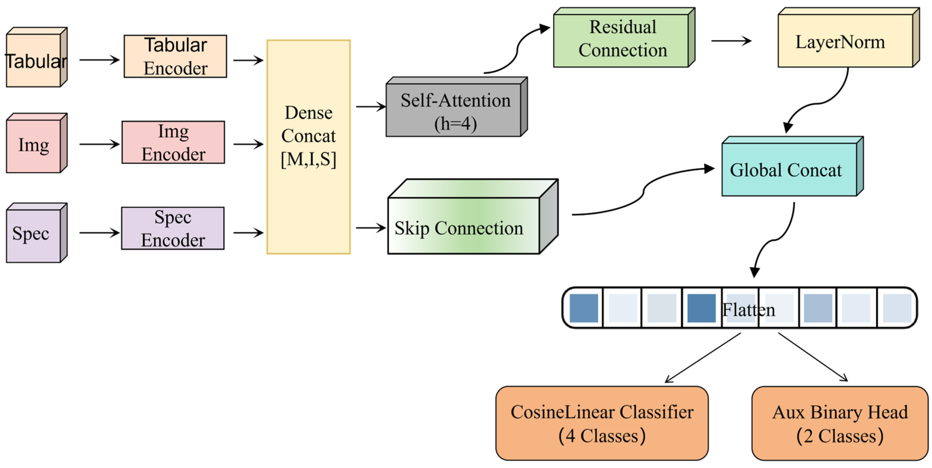
To address the issue of insufficient feature representation from a single modality, this paper proposes an end-to-end multi-modal feature fusion deep neural network named GCSNet. The network improves galaxy classification performance by effectively integrating complementary information from different modalities. In multi-modal galaxy classification research, using modality-specific encoders to extract intrinsic features from each modality is a common and effective strategy, as it avoids mutual interference between features from different modalities and better preserves the unique information of each modality [38]. Meanwhile, self-attention mechanisms, with their powerful capability for modeling global dependencies, have been widely adopted in cross-modal fusion tasks, effectively capturing latent correlations among features from different modalities and generating more discriminative fused features [39].

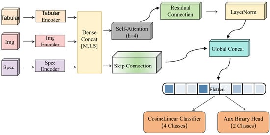
Accordingly, as shown in Figure 1, the GCSNet architecture mainly consists of three modality-specific encoders, a self-attention fusion module, and a dual-task classification head. The model extracts features from each modality using independent encoders and leverages the self-attention mechanism to generate fused features that contain global interaction information. To prevent the loss of shallow effective information during deep feature fusion, this paper introduces a skip connection structure that concatenates the original modality features with the deeply fused features, further improving the overall feature representation capability [40]. The concatenated features are then mapped onto a unit hypersphere via L2 normalization, and cosine similarity is used for primary classification. This strategy ensures that classification depends only on feature direction, free from interference caused by differences in feature magnitude, thereby enhancing the stability and accuracy of classification [41].

Figure 1. Overview of the multi-modal model architecture.

Composite galaxies lie on the BPT diagram in the transition region between star-forming galaxies and AGNs. Their characteristics exhibit a mixture of both types, leading to blurred boundaries and high classification difficulty. Furthermore, AGN samples account for a relatively small proportion in the dataset, making the model prone to bias toward the majority class and less sensitive to AGN identification. To address these issues, this paper introduces an auxiliary binary classification head for AGN/non-AGN discrimination. Through multi-task learning, the primary classification task and the AGN identification task are combined, leveraging complementary information between tasks to guide the model toward learning more generalizable feature representations [42]. This approach enhances the robustness of AGN recognition while indirectly improving the model’s ability to distinguish transitional samples such as composite galaxies, thereby improving overall classification performance. For reproducibility, the source code for GCSNet is available in the Supplementary Materials.

3.1. Image Encoder

Designed for efficient and robust feature extraction from two-dimensional photometric images, this module employs a lightweight 2D-CNN architecture comprising a stack of three convolutional modules. To ensure stable training dynamics and enhance non-linear representation capability, each convolutional layer is immediately followed by Batch Normalization (Batch Norm) and an ReLU activation function. Spatial dimensionality is reduced via a two-stage downsampling strategy, which halves the feature map resolution (height and width) at each stage. Concurrently, the channel depth is progressively expanded from 32 to 128; this design choice broadens the receptive field while capturing multi-level semantic features. Finally, following the third convolutional layer, a 4 × 4 adaptive average pooling layer (AdaptiveAvgPool2d) is applied to transform spatial features into 16 grid tokens (4 × 4). These tokens are then linearly projected into a 128-dimensional feature space to obtain the image feature sequence $F_{\mathrm{img}}\in R^{B\times 16\times 128}$, as illustrated in Figure 2. Here, B represents the batch size, 16 denotes the sequence length (number of tokens), and 128 signifies the feature dimension.

Figure 2. Schematic diagram of the Image Encoder.

3.2. Spectral Encoder

Designed specifically for one-dimensional spectral sequences, this module employs a three-layer 1D-CNN to capture local emission lines and continuous spectral characteristics. To effectively model features at multiple scales, the convolutional kernel sizes are set to 11, 7, and 5, with corresponding strides of 2, 2, and 1. The channel depth progressively increases from 1 to 128, enabling the extraction of hierarchical spectral representations. Each convolutional layer is followed by Batch Normalization and an ReLU activation function to stabilize training and enhance non-linearity. Finally, to handle variable-length input spectra, an AdaptiveAvgPool1d layer is applied to compress the features into a fixed sequence of 16 tokens, forming the final spectral feature sequence $F_{\mathrm{spec}}\in R^{B\times 16\times 128}$, as illustrated in Figure 3.

Figure 3. Schematic diagram of the Spectral Encoder.

3.3. Tabular Encoder

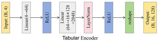
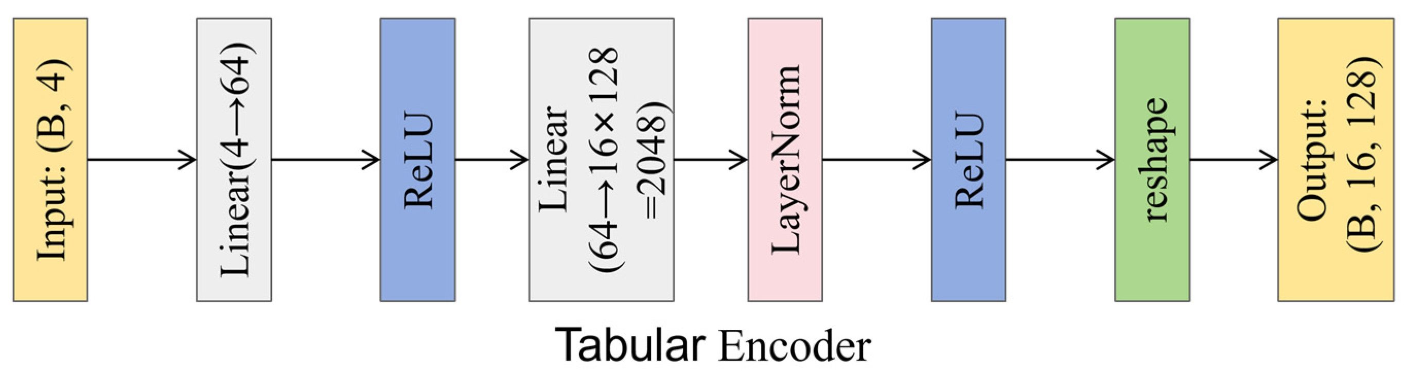
Designed for low-dimensional dense metadata vectors, this module employs a Multi-Layer Perceptron (MLP) to project sparse inputs into a high-dimensional latent space, effectively reshaping them into pseudo-sequences compatible with other modalities. The original metadata are first mapped to a 64-dimensional hidden space via two successive linear layers and then expanded to a total dimensionality of 2048 (16 × 128). Following Layer Normalization and ReLU activation, this feature vector is reshaped into a sequence format of (B, 16, 128), yielding the final metadata feature sequence $F_{\mathrm{meta}}\in R^{B\times 16\times 128}$, as illustrated in Figure 4.

Figure 4. Schematic diagram of the Tabular Encoder.

Although the three encoders adopt different architectures to adapt to the data characteristics of their respective modalities, they all standardize their outputs into a sequence representation of (B, 16, 128) via pooling or reshaping operations, ensuring the dimensional consistency of the subsequent fusion modules.

3.4. Multi-Modal Self-Attention Fusion Module

Information competition between modalities often causes simple feature concatenation to fail, where dominant modalities tend to mask the features of weaker ones [43]. Inspired by Dense Fusion [44], this study proposes a four-way self-attention fusion module based on the concept of dense feature-level fusion via pixel-wise correspondence. Unlike traditional global fusion strategies, Dense Fusion has demonstrated that fine-grained cross-modal interaction (e.g., at the pixel or token level) significantly enhances the model’s ability to capture local features and improves robustness. Specifically, the module first concatenates the output features from the three encoders along the sequence dimension, obtaining the total joint feature that contains $F_{\mathrm{spec}}$, $F_{\mathrm{img}}$, $F_{\mathrm{meta}}$ all the modal information from the three encoders. Subsequently, a 4-head multi-head self-attention mechanism is applied, enabling each token to attend to global dependencies across all other modalities. Following residual connection and Layer Normalization, the features are compressed back to 16 tokens via adaptive average pooling to obtain the global fused features $F_{\mathrm{fused}}\in R^{B\times 16\times 128}$. Finally, the fused features $F_{fused}$ are concatenated with the original output features from the three encoders to form the final complementary feature representation $F_{\mathrm{final}}=[F_{\mathrm{spec}},F_{\mathrm{img}},F_{\mathrm{meta}},F_{\mathrm{fused}}]\in R^{B\times 64\times 128}$. This design not only retains the original discriminative information of each mode (preventing information loss during fusion), but also introduces interactively enhanced fused features, significantly improving the expressive power of the features.

3.5. Cosine Similarity Classification Head

In multimodal fusion, the magnitude (norm) of feature vectors from different samples is often affected by non-semantic factors such as modality data quality, acquisition conditions, and signal-to-noise ratio. This means that even if two samples belong to the same category and have similar feature directions, their magnitudes may differ significantly. Traditional linear classifiers (i.e., fully connected layers with Softmax) are sensitive to feature magnitude and tend to mistakenly interpret magnitude differences as evidence for category discrimination, leading to fluctuating and unstable classification confidence. In contrast, the cosine similarity classifier first applies L2 normalization to both features and weights, comparing only their directions without being affected by magnitude variations. In this way, the classification result truly depends on the semantic direction derived from multimodal fusion, rather than fluctuations caused by data acquisition or quality. Moreover, this design requires no bias term, has fewer parameters, and is more stable in class-imbalanced scenarios [45].

Specifically, the fused features are first flattened into a vector of dimension 2048 × 4 = 8192. Both the input feature vector x and the weight vectors w are then subjected to L2 normalization, projecting them onto a unit hypersphere. The classification score is derived in two steps: first, the cosine similarity between the normalized vectors is calculated (Equation (6)); second, this value is multiplied by a learnable scaling factor σ (initialized to 30.0) to yield the final logits (Equation (7)), where x denotes the input feature vector and w represents the weight vector.

$$\cos (x,w)={\displaystyle \frac{x\cdot w}{‖x‖‖w‖}}$$

(6)

$$\mathrm{logits}=\sigma \cdot \cos (x,w)$$

(7)

This mechanism ensures that classification decisions rely solely on the direction of the feature vectors, effectively eliminating interference from amplitude factors (such as brightness) and enhancing the model’s ability to distinguish subtle inter-class differences. Regarding data augmentation, to address the long-tail distribution [46] inherent in the observed galaxy data, a weighted random sampler was integrated into the training data loader. The sampling weight for each sample is determined by the reciprocal of its class frequency, where $n_{c(i)}$ denotes the total number of samples in the category c(i) to which the i-th sample belongs.

$$w_i={\displaystyle \frac{1}{n_{c(i)}}}$$

(8)

Additionally, based on the BPT diagram, galaxy classification is not completely discrete, and intrinsic physical connections exist between different classes. From star-forming galaxies, to composite galaxies, AGNs, and finally normal galaxies, there is a continuous physical transition. This physical continuum means that there are no sharp, well-defined boundaries between classes. In this context, Mixup [47] smooths decision boundaries via convex combinations of training samples, and such linear interpolation is naturally suited to classification tasks where classes form a continuum [48]. The Mixup data augmentation technique is employed to generate new training samples by blending two images and their corresponding labels in specific proportions. Specifically, two samples, (X₁, y₁) and (X₂, y₂), are randomly selected, where X = (image, spectrum, tabular data), y denotes the label. To maintain modality consistency, the same mixing coefficient $\lambda$ is applied across the image, spectral, and metadata inputs when generating the new samples $\tilde{X}$. The formulation is presented in Equation (9).

$$\tilde{X}=\lambda X_1+(1-\lambda )X_2,\tilde{y}=\lambda y_1+(1-\lambda )y_2$$

(9)

4. Results and Discussion

To comprehensively evaluate the effectiveness and robustness of the proposed multimodal feature fusion framework, GCSNet, this section presents extensive performance validation experiments and ablation studies. Through a rigorous experimental design covering diverse metrics and scenarios, we demonstrate the superiority of our multi-modal fusion approach over single-modal baselines. Furthermore, the results highlight the significant advantages of our proposed architecture in terms of both classification accuracy and robustness.

4.1. Evaluation Indicators

All experiments were conducted under identical hardware and software environments to ensure the comparability and reproducibility of the results. Specifically, the following core evaluation metrics were employed to verify the model’s robustness, as defined in Equations (10)–(13):

(1)

Accuracy: Overall classification accuracy.

$$Accuracy={\displaystyle \frac{TP+TN}{TP+TN+FP+FN}}$$

(10)

(2)

Precision: The accuracy of predicting each category as positive.

$$\mathrm{Pr}\mathrm{e}cision={\displaystyle \frac{TP}{TP+FP}}$$

(11)

(3)

Recall: The detection rate of actual positive cases in each category.

$$\mathrm{Re}\mathrm{c}all={\displaystyle \frac{TP}{TP+FN}}$$

(12)

(4)

F1-score: The harmonic average of precision and recall.

$$\mathrm{F}1-\mathrm{score}=2\times {\displaystyle \frac{\mathrm{Precision}\times \mathrm{Recall}}{\mathrm{Precision}+\mathrm{Recall}}}$$

(13)

(5)

AUC value: The area under the ROC curve, which measures the overall discriminative ability of the model. The value ranges from 0 to 1, with values closer to 1 indicating better performance.

4.2. Experimental Setup

4.2.1. Hardware and Training Configuration

All experiments were conducted on a server running CentOS 7.9, equipped with 256 GB memory and 4 NVIDIA A100 (80 GB) GPUs. The model was implemented in Python 3.8 using PyTorch 2.0.1.

We trained the model from scratch for 120 epochs with a batch size of 64. The AdamW optimizer was used with an initial learning rate of 0.001, weight decay of 0.001, and label smoothing of 0.1. The total training time was approximately 30 h on a single A100 GPU (30 GPU hours).

4.2.2. Baseline Models

To systematically verify the effectiveness of the proposed method, the experimental design is divided into two categories: single-modal baselines and multi-modal fusion groups.

The single-modal baseline group aims to reveal that although single-modal classification methods are mature, they are limited by the partial nature of single data sources and struggle to achieve comprehensive characterization of complex galaxies. We selected GaSNet [10] as a highly representative pure spectral baseline model. Proposed by Zhong et al., this model is based on a multi-channel ensemble system that utilizes multiple small ResNet sub-networks with independent initial weights to process 1D spectral data, demonstrating superior performance in spectral classification tasks. In addition, we introduced the spectral branch of the transfer learning model (ISTL) [49] proposed by Wang and Hong et al. (2023) to compare and evaluate the performance differences in different spectral feature extractors. Notably, to verify the effectiveness of the spectral branch proposed in this paper and to provide a reference for the subsequent improvement in multi-modal classification capability, the GCSNet spectral branch is also included in this baseline group.

The multi-modal fusion group focuses on exploring the pros and cons of different fusion mechanisms to verify the superiority of the GCSNet fusion strategy. This group introduces MB-ISTL [49] as a representative traditional dual-modal model. This method independently extracts spectral and image features and then fuses them at the decision level via concatenation and weighting, representing a classic late fusion paradigm. Meanwhile, we referenced the TransformerFusion [50] model proposed by Gao et al. (2023). This model utilizes the self-attention mechanism of a multi-modal Transformer to achieve cross-modal interaction at the embedding sequence level, representing a state-of-the-art fusion method. On this basis, we established two core comparisons: first, the proposed end-to-end dual-modal architecture (Spectral–Image Dual-Modal), which serves as a baseline for data alignment in multi-modal tasks; and second, the final proposed tri-modal fusion model, GCSNet, which incorporates tabular data features to better supplement multi-dimensional galaxy information and further break through existing performance bottlenecks.

4.3. Comparative Experiment

4.3.1. Multi-Class Galaxy Classification Performance Evaluation

Galaxy classification faces the dual challenges of high-dimensional data and feature sparsity, making it difficult to capture the full physical picture using a single feature source. Effective fusion architectures can mitigate the limitations of single-modality data by integrating heterogeneous multi-source information, thereby significantly enhancing classification accuracy. Accordingly, we conducted a systematic comparative study to evaluate the fine-grained classification performance of various models across four galaxy types: AGNs, Star-Forming, Composite, and Normal. Table 2 summarizes the quantitative results in terms of Precision, Recall, and F1-score.

Table 2. Performance Evaluation for Four-Class Galaxy Classification.

Model	Class	Precision	Recall	F1-Score
GaSNet	AGN	94.75%	94.17%	94.46%
	STAR FORMING	98.33%	96.88%	97.60%
	Composite	89.17%	92.74%	90.92%
	Normal	99.60%	99.69%	99.64%
	Average	95.46%	95.87%	95.65%
MB-ISTL	AGN	90.53%	93.99%	92.23%
	STAR FORMING	97.83%	93.69%	95.71%
	Composite	82.31%	89.29%	85.66%
	Normal	99.69%	99.69%	99.69%
	Average	92.59%	94.17%	93.32%
Transformer	AGN	94.71%	93.76%	94.23%
	STAR FORMING	96.63%	96.72%	96.67%
	Composite	88.29%	88.43%	88.32%
	Normal	99.76%	99.85%	99.81%
	Average	94.85%	94.69%	94.76%
GCSNet	AGN	93.80%	96.17%	94.97%
	STAR FORMING	97.72%	98.72%	98.22%
	Composite	94.34%	90.56%	92.41%
	Normal	100.00%	99.96%	99.98%
	Average	96.47%	96.35%	96.39%

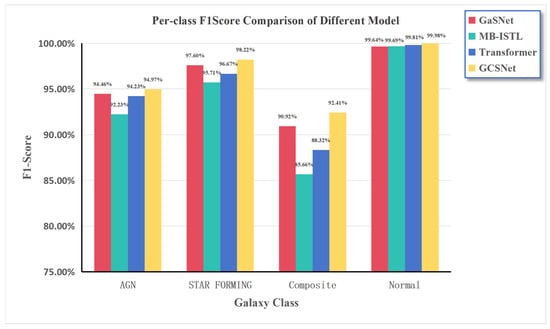
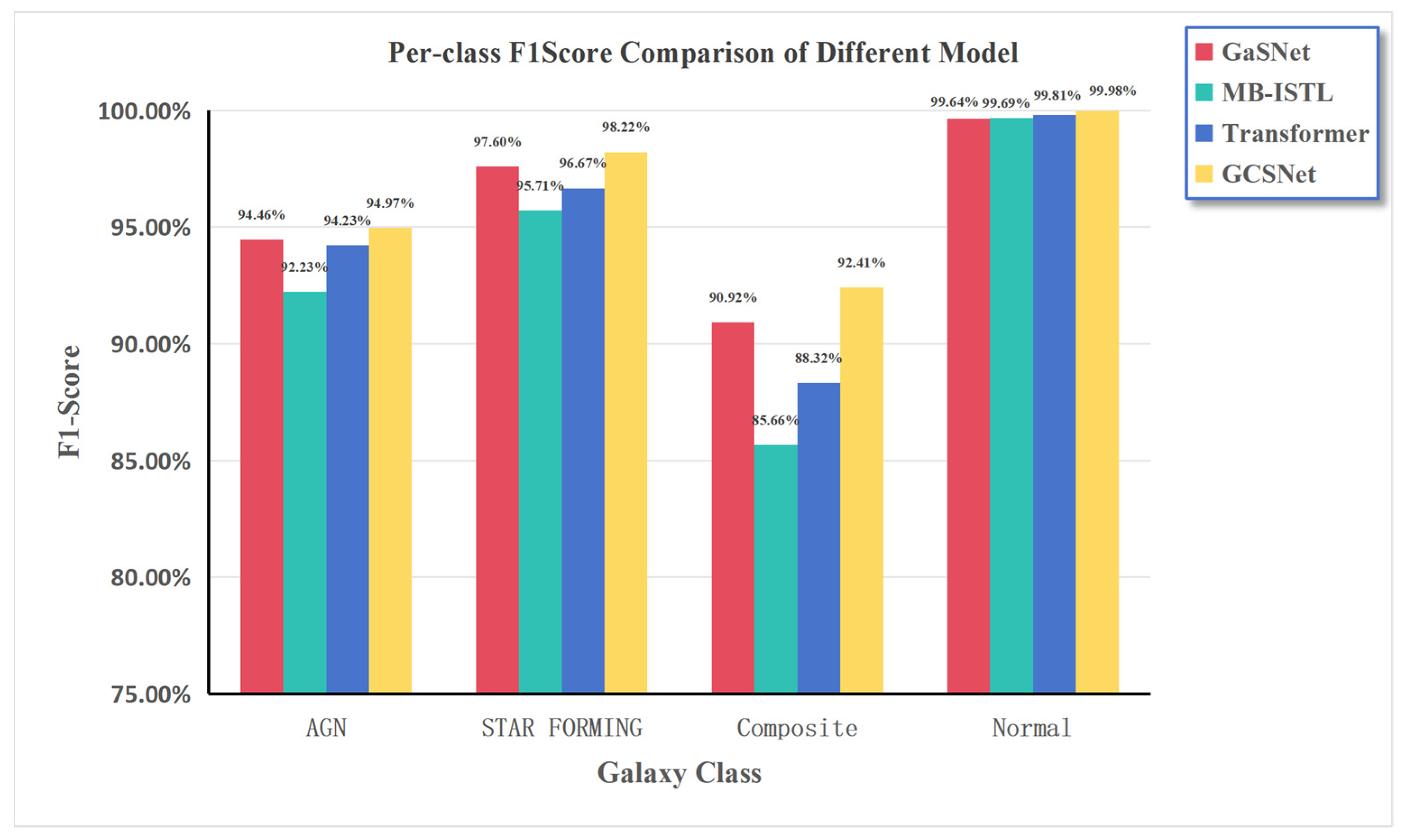
The F1-score combines recall and precision, providing a more comprehensive reflection of classification performance across different categories compared to a single metric. Figure 5 presents an intuitive comparison of F1-scores for each galaxy type across different models in the form of a bar chart.

Figure 5. Per-class F1 score comparison of different models on galaxy classification.

The results indicate that model classification performance is highly correlated with the distinctiveness of galactic physical features and sample abundance: categories with unique features and sufficient samples yield superior classification results, whereas high spectral feature overlap significantly increases classification difficulty.

Normal Galaxies: All models performed exceptionally well on this category, attributable to its distinct physical characteristics. Normal galaxies exhibit weak or absent emission lines, resulting in clear boundaries from other categories in the BPT diagnostic diagram. Notably, GCSNet, leveraging its multi-modal fusion strategy, further eliminated misclassifications, achieving a precision of 100%.

Star-Forming Galaxies: Benefiting from abundant samples and prominent spectral features, all models demonstrated strong learning capability for this category. The best performance was observed in GCSNet and the single-spectrum model GaSNet. Although GCSNet’s accuracy was marginally lower than GaSNet’s (by 0.6%), it achieved a 2% higher recall and a 1% higher F1-score, indicating superior comprehensive performance.

Composite and AGN Galaxies: Classification performance for these categories was relatively poor, primarily due to their prominent strong emission-line features. Particularly for composite galaxies, which reside in the transition region between star formation and AGN on the BPT diagram, the ambiguous spectral boundaries make them highly prone to confusion. The proposed GCSNet effectively mitigates this issue, achieving a classification accuracy of 94.34%, which outperforms the second-best model by 5.18%.

4.3.2. Overall Model Performance Evaluation

Based on the detailed analysis of individual galaxy types, this section presents a comprehensive comparison of the overall performance of all models, with a focus on evaluating the impact of different fusion strategies on classification accuracy. The results are summarized in Table 3.

Table 3. Comparison of experimental results across different models.

Model	Accuracy	Precision	Recall	F1-Score
GaSNet	96.39%	95.46%	95.87%	95.65%
ISTL (Spectral)	93.52%	91.50%	94.15%	92.70%
our-Spectral	96.14%	95.68%	96.21%	95.95%
MB-ISTL	94.18%	92.59%	94.17%	93.32%
TransformerFusion	95.49%	94.85%	94.69%	94.76%
our-Spec_Img	96.02%	95.57%	95.57%	95.57%
GCSNet	97.15%	96.47%	96.35%	96.39%

Results analyses and experimental data demonstrate two key findings: (1) Single-modality classification methods are highly mature, with GaSNet achieving a high accuracy of 96.39% using only spectral features; (2) some existing multi-modality methods perform even worse than the single-modality baseline due to improper fusion strategies, such as shallow concatenation or modality inconsistency. In contrast, GCSNet, by designing a reasonable and effective fusion strategy and leveraging multi-dimensional feature data of galaxies, achieves optimal performance across all metrics in terms of overall performance.

As shown in Table 4, GCSNet outperforms the compared models across all evaluation metrics, achieving an AUC value closest to 1. This indicates that its discriminative ability for each category is superior to that of the compared models, further demonstrating the model’s robustness and generalization capability in classification tasks.

Table 4. AUC evaluation results of different models on the four-class classification task.

Model	GCSNet	GaSNet	Our-Spec_Img	TransformerFusion	Our-Spectral	MB-ISTL	Spectral
AUC	0.9967	0.9967	0.9961	0.9956	0.9954	0.9945	0.9938

Note: Although both GCSNet and GaSNet show an AUC of 0.9967 in the table, GCSNet achieves a slightly higher value when considering more decimal places (0.996675 vs. 0.996664).

4.3.3. Model Stability Evaluation

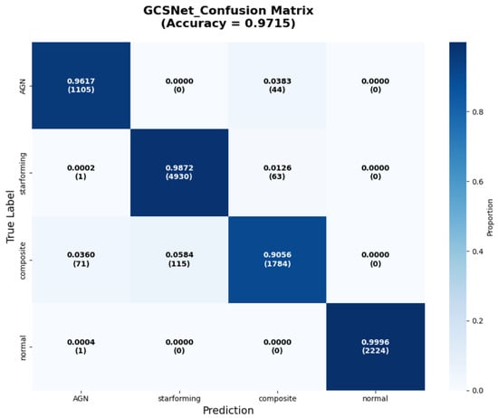
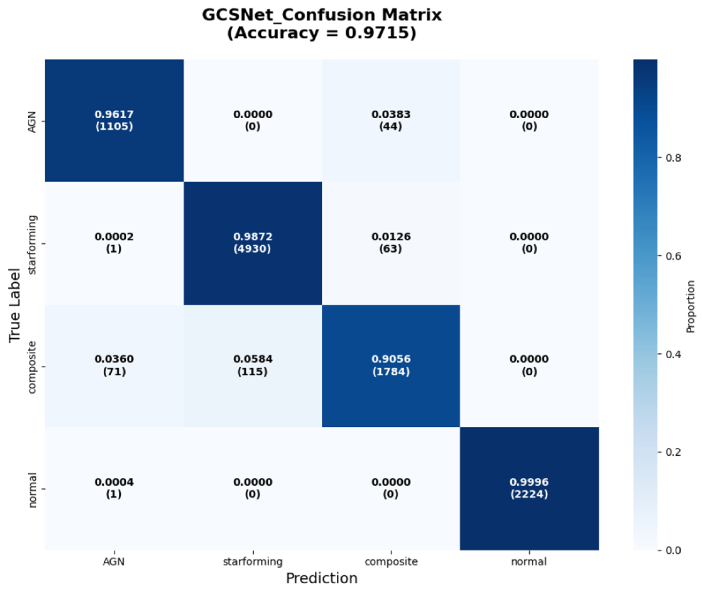
The experimental results above demonstrate that GCSNet achieves the best overall performance among the compared models. To further evaluate the model’s fine-grained discriminative capability across different galaxy categories, this study conducted three independent repeated experiments with multiple random seeds. Table 5 (four-class evaluation metrics) and Figure 6 (confusion matrix) present a detailed illustration of the model’s classification performance and stability.

Table 5. Per-class classification performance of GCSNet (mean ± std over 3 runs).

Class	Precision	Recall	F1-Score
AGN	94.09% ± 0.67%	96.03% ± 1.05%	95.05% ± 0.61%
STAR FORMING	98.33% ± 0.27%	97.92% ± 0.42%	98.13% ± 0.09%
Composite	92.50% ± 1.56%	92.32% ± 1.02%	92.40% ± 0.53%
Normal	100.00% ± 0.03%	100.00% ± 0.00%	99.99% ± 0.01%

Note: All metrics are reported as the mean ± standard deviation of three independent experiments (random seeds: 42, 100, 3407).

Figure 6. GCSNet confusion matrix.

As shown in Table 5, GCSNet demonstrates excellent performance in the four-class galaxy classification task. The standard deviations ranging from 0.006 to 0.016 confirm the model’s high stability and strong robustness.

The clear diagonal distribution observed in the confusion matrix (Figure 6) confirms the model’s effectiveness in distinguishing morphologically similar galaxies, with minimal inter-class confusion. The sparse misclassifications in the off-diagonal regions are primarily concentrated on boundary samples with ambiguous features (e.g., between AGNs and composite galaxies). This pattern indicates that the errors stem from the inherent ambiguity of the samples themselves rather than any systematic bias in the model. Overall, the combined chart data further demonstrates the model’s superior performance in the galaxy classification task.

4.4. Ablation Experiment

To systematically evaluate the contribution of each module to the final performance of the model, we designed multiple sets of ablation experiments. We observed their influence on the best validation accuracy and the final test accuracy in two scenarios: obs (original observed spectra) and rest (rest-frame spectra).

(1)

Observation Scene (Obs)

Table 6 presents the experimental results under the condition of retaining complete tabular data input (including redshift information). Among all configurations, obs/all (image + observed-frame spectra + tabular data with redshift) achieves the best performance, validating the effectiveness of full-modal integration.

Table 6. Verification experiments for observing the original spectrum.

Frame	Ablation	Best_Val_Acc	Final_Test_Acc
obs	all	97.21%	97.19%
obs	all_noz	96.55%	96.90%
obs	spec_img	96.21%	96.32%
obs	spec_tabular_ewonly	96.80%	96.74%
obs	spec_tabular_noew	96.64%	96.77%
obs	spec_tabular_noz	96.70%	97.00%
obs	spec_only	96.20%	96.37%
obs	spec_tabular	97.05%	97.19%
obs	all_noebmv	97.14%	97.18%
obs	all_noz_noebmv	96.81%	96.91%
obs	spec_tabular_noz_noebmv	96.89%	96.78%

Note: Bold entries in the table highlight the best results in the obs scenario, demonstrating the superiority of full modality integration.

(2)

Redshift removal scene (Rest)

The rest setting in Table 7 removes redshift from the spectra, simulating two extreme scenarios: (1) low-SNR spectra where redshift cannot be accurately measured, and (2) cross-domain transfer to datasets lacking redshift labels.

Table 7. Verification Experiments of redshift spectra.

Frame	Ablation	Best_Val_Acc	Final_Test_Acc
rest	all	95.14%	94.84%
rest	all_noz	95.26%	95.05%
rest	spec_img	94.79%	94.70%
rest	spec_tabular_ewonly	95.04%	94.72%
rest	spec_tabular_noew	94.89%	94.49%
rest	spec_tabular_noz	95.03%	95.05%
rest	spec_only	94.82%	94.75%
rest	spec_tabular	95.27%	94.85%
rest	all_noebmv	95.25%	94.92%
rest	all_noz_noebmv	95.00%	94.85%
rest	spec_tabular_noz_noebmv	94.91%	94.82%

Note: Bold entries highlight the best results in the redshift removal (Rest) scenario, demonstrating the superiority of full-modal integration without redshift information (all_noz).

The comparison between Table 6 and Table 7 reveals the following findings. In the observed-frame spectral setting (obs) where redshift is retained, the complete three-source model achieves the best performance (0.972142), validating the effectiveness of full-modal fusion. In contrast, all models exhibit a general performance drop in the redshift-removed (rest) setting, indicating that redshift serves as an important physical prior for galaxy classification, effectively constraining the feature space and assist in distinguishing galaxies with similar morphology but different evolutionary stages.

Notably, under the rest-frame spectral condition (rest, where spectral line shifts are removed), the configuration with redshift included in the tabular data (rest/all, 94.84%) performs worse than the version without redshift (rest/all_noz, 95.05%). This suggests that when the spectra no longer provide redshift-related spectral line shift information, the tabular redshift value cannot form effective complementarity, and repeatedly inputting the same physical quantity leads to information redundancy or interference.

In summary, redshift should be used as an independent but non-redundant prior feature. When the spectra retain the redshift effect, it works synergistically with the tabular redshift. However, once the spectra are de-redshifted, additional redshift input is no longer beneficial. These ablation results further confirm that redshift not only improves classification accuracy but also enhances the model’s ability to utilize physical evolution information, provided that its input is based on the principle of information complementarity.

5. Conclusions

This paper proposes GCSNet, a multimodal deep learning framework that deeply fuses image morphology, spectral physics, and tabular statistical features, achieving a classification accuracy of 97.15%, significantly outperforming existing single-modal and multimodal models. Beyond improving classification accuracy, the model reveals the physical complementary mechanisms among different modalities in galaxy classification. The fusion of the three modalities effectively mitigates the ambiguity encountered by single-modality approaches when handling boundary samples, particularly for galaxies with similar morphology but different physical states (e.g., composites and AGNs).

Furthermore, this study reveals the impact of galaxy physical characteristics and sample abundance on classification performance. Normal galaxies, characterized by clear spectral features (weak or absent emission lines) and sufficient samples, achieve 100% precision with GCSNet. In contrast, composite galaxies and AGNs, located in the transition region of the BPT diagram with blurred spectral boundaries, are more difficult to classify. Nevertheless, GCSNet achieves 94.34% accuracy on composite galaxies, a 5.18% improvement over the next-best model (GasNet).

In summary, GCSNet demonstrates strong classification capability, validates the significant potential of multimodal learning in astronomical data mining, and provides a high-precision solution for automated galaxy classification.

6. Limitations and Future Work

Although GCSNet achieves excellent classification performance, several limitations remain in this study. First, to ensure the reliability of BPT-based classification labels, both the training and test samples are restricted to galaxies with redshift 0 < z < 0.3. Consequently, the generalization capability of the model to higher redshifts remains to be verified. Second, cross-survey validation has not yet been conducted on large-scale survey datasets such as LSST, CSST, Euclid, and DESI, leaving the robustness of the model on these datasets untested. Third, the model relies to some extent on redshift information as a prior, and there is a risk of performance degradation in extreme scenarios where redshift is missing (e.g., low signal-to-noise ratio spectra).

To address the above limitations, future work will focus on the following three aspects: (1) extending the model to higher redshifts by adopting classification standards suitable for high-redshift galaxies (e.g., [OIII]/Hβ, line width, velocity dispersion, etc.); (2) conducting cross-survey validation on the aforementioned survey samples to systematically evaluate the model’s generalization ability and robustness; and (3) exploring robust classification methods based on image and spectral morphology for scenarios with missing redshift information, thereby reducing the model’s dependence on the redshift prior.

References

- Hubble, E.P. Extragalactic nebulae. Astrophys. J. 1926, 64, 321–369. [Google Scholar] [CrossRef] [Scilit]
- Odewahn, S.C.; Stockwell, E.B.; Pennington, R.L.; Humphreys, R.M.; Zumach, W.A. Automated star/galaxy discrimination with neural networks. Astron. J. 1992, 103, 318–331. [Google Scholar] [CrossRef] [Scilit]
- Dai, J.M. Research on Galaxy Morphological Classification Based on Deep Convolutional Neural Networks. Master’s Thesis, University of Chinese Academy of Sciences (National Space Science Center, Chinese Academy of Sciences), Beijing, China, 2018. [Google Scholar]
- Yang, Y.; Wen, Z.L.; Xia, J.Q. Star-galaxy classifier based on residual neural networks. J. Beijing Norm. Univ. (Nat. Sci.) 2021, 57, 450–457. [Google Scholar]
- Kong, X.Y.; Dou, J.P. Galaxy morphology classification model based on SE-Inception-v3. Acta Astron. Sin. 2024, 65, 30–43. [Google Scholar]
- Wu, J.F.; Walmsley, M. Re-envisioning Euclid Galaxy Morphology: Identifying and Interpreting Features with Sparse Autoencoders. arXiv 2025, arXiv:2510.23749. [Google Scholar] [CrossRef] [Scilit]
- Baldwin, J.A.; Terlevich, M.M.P. Classification parameters for the emission-line spectra of extragalactic objects. Publ. Astron. Soc. Pac. 1981, 93, 5–19. [Google Scholar] [CrossRef] [Scilit]
- Connolly, A.J.; Szalay, A.S.; Bershady, M.A.; Kinney, A.L.; Calzetti, D. Spectral classification of galaxies: An orthogonal approach. Astron. J. 1995, 110, 1071. [Google Scholar] [CrossRef] [Scilit]
- Wu, Y.; Tao, Y.; Fan, D.; Cui, C.; Zhang, Y. Galaxy spectral classification and feature analysis based on convolutional neural network. Mon. Not. R. Astron. Soc. 2023, 527, 1163–1176. [Google Scholar] [CrossRef] [Scilit]
- Zhong, F.; Napolitano, N.R.; Caroline, H.; Rui, L.; Erik, B.F.; Nicolas, B.; Johan, C.; Young-Lo, K.; Jens-Kristian, K.; Marcella, L. Galaxy Spectra neural Network (GaSNet). II. Using deep learning for spectral classification and redshift predictions. Mon. Not. R. Astron. Soc. 2024, 532, 643–665. [Google Scholar] [CrossRef] [Scilit]
- Wu, J.F.; Boada, S. Using convolutional neural networks to predict galaxy metallicity from three-colour images. Mon. Not. R. Astron. Soc. 2019, 484, 4683–4694. [Google Scholar] [CrossRef] [Scilit]
- Wu, J.F.; Peek, J.E.G. Predicting galaxy spectra from images with hybrid convolutional neural networks. arXiv 2020, arXiv:2009.12318. [Google Scholar] [CrossRef] [Scilit]
- Holwerda, B.W.; Wu, J.F.; Keel, W.C.; Young, J.; Mullins, R.; Hinz, J.; Ford, K.E.S.; Barmby, P.; Chandar, R.; Bailin, J.; et al. Predicting the Spectrum of UGC 2885, Rubin’s Galaxy with Machine Learning. Astrophys. J. 2021, 914, 142. [Google Scholar] [CrossRef] [Scilit]
- Alfonzo, J.P.; Iyer, K.G.; Akiyama, M.; Bryan, G.L.; Cooray, S.; Ludwig, E.; Mowla, L.; Omori, K.C.; Pacifici, C.; Speagle, J.S.; et al. Katachi: Decoding the Imprints of Past Star Formation on Present-day Morphology in Galaxies with Interpretable CNNs. Astrophys. J. 2024, 967, 152. [Google Scholar] [CrossRef] [Scilit]
- Wei, J.; Jiang, B.; Zhang, Y. Identification of Blue Horizontal Branch Stars with Multimodal Fusion. Publ. Astron. Soc. Pac. 2023, 135, 084501. [Google Scholar] [CrossRef] [Scilit]
- Deng, Z.J.; Yu, S.Y.; Luo, A.; Kong, X.; Li, X.R. Ensemble Learning for Stellar Classification and Radius Estimation from Multimodal Data. Res. Astron. Astrophys. 2024, 24, 211–224. [Google Scholar] [CrossRef] [Scilit]
- Rizhko, M.; Bloom, J.S. AstroM3: A self-supervised multimodal model for astronomy. Astron. J. 2024, 170, 28. [Google Scholar] [CrossRef] [Scilit]
- Junell, A.; Sasli, A.; Nunes, F.F.; Xu, M.; Border, B.; Rehemtulla, N.; Rizhko, M.; Qin, Y.J.; Laz, T.J.D.; Calloch, A.L. Applying multimodal learning to Classify transient Detections Early (AppleCiDEr) I: Data set, methods, and infrastructure. arXiv 2025, arXiv:2507.16088. [Google Scholar] [CrossRef] [Scilit]
- Brinchmann, J.; Charlot, S.; White, S.D.M.; Tremonti, C.; Kauffmann, G.; Heckman, T.; Brinkmann, J. The physical properties of star-forming galaxies in the low-redshift Universe. Mon. Not. R. Astron. Soc. 2010, 351, 1151–1179. [Google Scholar] [CrossRef] [Scilit]
- Kauffmann, G.; Heckman, T.M.; White, S.D.M.; Charlot, S.; Tremonti, C.; Brinchmann, J.; Bruzual, G.; Peng, E.W.; Seibert, M.; Bernardi, M.; et al. Stellar masses and star formation histories for 105 galaxies from the Sloan Digital Sky Survey. Mon. Not. R. Astron. Soc. 2003, 34, 33–53. [Google Scholar] [CrossRef] [Scilit]
- Wang, B.Z. Discussion on characteristics, classification and unified model of active galactic nuclei. J. Jiaozuo Teach. Coll. 2025, 41, 74–76. [Google Scholar]
- Baldry, I.K.; Glazebrook, K.; Brinkmann, J.; Ivezi, E.; Lupton, R.H.; Nichol, R.C.; Szalay, A.S. Quantifying the Bimodal Color-Magnitude Distribution of Galaxies. Astrophys. J. 2004, 600, 681–694. [Google Scholar] [CrossRef] [Scilit]
- Chamorro-Cazorla, M.; De Paz, A.G.; Castillo-Morales, A.; Camps-Fariña, A.; Gallego, J.; Carrasco, E.; Iglesias-Pramo, J.; Cedazo, R.; Garca-Vargas, M.L.; Pascual, S. MEGADES: MEGARA galaxy disc evolution survey. Ionised gas diagnosis. Astron. Astrophys. 2025, 705, A53. [Google Scholar] [CrossRef] [Scilit]
- Salton, G. A vector space model for automatic indexing. Commun. ACM 1975, 18, 613–620. [Google Scholar] [CrossRef] [Scilit]
- Abdurro’uf; Accetta, K.; Aerts, C.; Silva Aguirre, V.; Ahumada, R.; Ajgaonkar, N.; Filiz Ak, N.; Alam, S.; Allende Prieto, C.; Almeida, A.; et al. The Seventeenth Data Release of the Sloan Digital Sky Surveys: Complete Release of MaNGA, MaStar and APOGEE-2 Data. Astrophys. J. Suppl. Ser. 2021, 259, 35. [Google Scholar] [CrossRef] [Scilit]
- Ball, N.M.; Brunner, R.J.; Myers, A.D.; Tcheng, D. Robust Machine Learning Applied to Astronomical Data Sets. I. Star-Galaxy Classification of the Sloan Digital Sky Survey DR3 Using Decision Trees. Astrophys. J. 2012, 650, 497–509. [Google Scholar] [CrossRef] [Scilit]
- Shirazi, M.; Brinchmann, J. Strongly star forming galaxies in the local Universe with nebular Heiiλ4686 emission. Mon. Not. R. Astron. Soc. 2012, 421, 1043–1063. [Google Scholar] [CrossRef] [Scilit]
- Willick, J.A. Measurement of Galaxy Distances. arXiv 1996, arXiv:astro-ph/9610200. [Google Scholar] [CrossRef] [Scilit]
- Dobos, L.; Csabai, I.; Yip, C.W.; Budavári, T.; Szalay, A.S. A high-resolution atlas of composite Sloan Digital Sky Survey galaxy spectra. Mon. Not. R. Astron. Soc. 2011, 420, 1217–1238. [Google Scholar] [CrossRef] [Scilit]
- Schlegel, D.J.; Finkbeiner, D.P.; Davis, M. Maps of Dust Infrared Emission for Use in Estimation of Reddening and Cosmic Microwave Background Radiation Foregrounds. Astrophys. J. 2009, 500, 525. [Google Scholar] [CrossRef] [Scilit]
- Kennicutt, R.C.; Ii, N.J.E. Star Formation in the Milky Way and Nearby Galaxies. Annu. Rev. Astron. Astrophys. 2012, 50, 531–608. [Google Scholar] [CrossRef] [Scilit]
- Strateva, I.; Ivezic, Z.; Knapp, G.R.; Narayanan, V.K.; Strauss, M.A. Color Separation of Galaxy Types in the Sloan Digital Sky Survey Imaging Data. Astron. J. 2001, 122, 1861–1874. [Google Scholar] [CrossRef] [Scilit]
- Liu, M.Y.; Zhao, Z.X.; Wang, W.; Zhao, W.H.; Cao, Z.T.; Zhao, S.W. Analysis and information extraction of LAMOST stellar spectra FITS files. Comput. Program. Ski. Maint. 2019, 5, 27–30. [Google Scholar]
- He, Z.; Qiu, B.; Luo, A.L.; Shi, J.; Kong, X.; Jiang, X. Deep Learning Applications Based on SDSS Photometric Data: Detection and Classification of Sources. Mon. Not. R. Astron. Soc. 2021, 508, 2039–2052. [Google Scholar] [CrossRef] [Scilit]
- Smee, S.A.; Gunn, J.E.; Uomoto, A.; Roe, N.; Schlegel, D.; Rockosi, C.M.; Carr, M.A.; Leger, F.; Dawson, K.S.; Olmstead, M.D.; et al. The multi-object, fiber-fed spectrographs for the sloan digital sky survey and the baryon oscillation spectroscopic survey. Astron. J. 2013, 146, 32. [Google Scholar] [CrossRef] [Scilit]
- Kewley, L.J.; Dopita, M.A.; Sutherland, R.S.; Heisler, C.A.; Trevena, J. Theoretical Modeling of Starburst Galaxies. Astrophys. J. 2001, 556, 121–140. [Google Scholar] [CrossRef] [Scilit]
- Collaboration, T.M.U.; Audenaert, J.; Bowles, M.; Boyd, B.M.; Chemaly, D.; Cherinka, B.; Ciuc, I.; Cranmer, M.; Do, A.; Grayling, M. The Multimodal Universe: Enabling Large-Scale Machine Learning with 100TB of Astronomical Scientific Data. Adv. Neural Inf. Process. Syst. 2024, 37, 57841–57913. [Google Scholar]
- Parker, L.; Lanusse, F.; Shen, J.; Liu, O.; Hehir, T.; Sarra, L.; Meyer, L.; Bowles, M.; Wagner-Carena, S.; Qu, H. AION-1: Omnimodal Foundation Model for Astronomical Sciences. Adv. Neural Inf. Process. Syst. 2025, 38, 95386–95428. [Google Scholar]
- Vaswani, A.; Shazeer, N.; Parmar, N.; Uszkoreit, J.; Jones, L.; Gomez, A.N.; Kaiser, L.; Polosukhin, I. Attention Is All You Need. arXiv 2017, arXiv:1706.03762. [Google Scholar]
- He, K.; Zhang, X.; Ren, S.; Sun, J. Deep Residual Learning for Image Recognition. In Proceedings of the IEEE Conference on Computer Vision and Pattern Recognition, Las Vegas, NV, USA, 27–30 June 2016. [Google Scholar]
- Wang, H.; Wang, Y.; Zhou, Z.; Ji, X.; Gong, D.; Zhou, J.; Li, Z.; Liu, W. CosFace: Large Margin Cosine Loss for Deep Face Recognition. In Proceedings of the IEEE Conference on Computer Vision and Pattern Recognition, Salt Lake City, UT, USA, 18–23 June 2018. [Google Scholar]
- Zhang, Y.; Yang, Q. A Survey on Multi-Task Learning. IEEE Trans. Knowl. Data Eng. 2021, 34, 5586–5609. [Google Scholar] [CrossRef] [Scilit]
- Baltrusaitis, T.; Ahuja, C.; Morency, L.P. Multimodal Machine Learning: A Survey and Taxonomy. IEEE Trans. Pattern Anal. Mach. Intell. 2018, 41, 423–443. [Google Scholar] [CrossRef] [Scilit]
- Wang, C.; Xu, D.; Zhu, Y.; Martín-Martín, R.; Lu, C.; Fei-Fei, L.; Savarese, S. DenseFusion: 6D Object Pose Estimation by Iterative Dense Fusion. In Proceedings of the IEEE/CVF Conference on Computer Vision and Pattern Recognition, Seattle, WA, USA, 13–19 June 2020. [Google Scholar]
- Xu, Y.; Lyu, C. Class-Balanced Regularization for Long-Tailed Recognition. Neural Process. Lett. 2024, 56, 158. [Google Scholar] [CrossRef] [Scilit]
- Cui, Y.; Jia, M.; Lin, T.Y.; Song, Y.; Belongie, S. Class-Balanced Loss Based on Effective Number of Samples. arXiv 2019, arXiv:1901.05555. [Google Scholar] [CrossRef] [Scilit]
- Zhang, H.; Cisse, M.; Dauphin, Y.N.; Lopez-Paz, D. mixup: Beyond Empirical Risk Minimization. arXiv 2017, arXiv:1710.09412. [Google Scholar]
- Shui, H.; Li, H.; Upadhyay, D.; Narayanan, P.; Admasu, A.S. Mixup for Robust Image Classification—Application in Continuously Transitioning Industrial Sprays. In Proceedings of the First Workshop on Interpolation Regularizers and Beyond at NeurIPS, New Orleans, LA, USA, 28 November–9 December 2022. [Google Scholar]
- Wang, B.; Hong, S.; Yuan, Z.; Luo, A.L.; Kong, X.; Zou, Z. A Multimodal Transfer Learning Method for Classifying Images of Celestial Point Sources. Publ. Astron. Soc. Pac. 2023, 135, 104502. [Google Scholar] [CrossRef] [Scilit]
- Gao, J.; Chen, J.; Wei, J.; Jiang, B.; Luo, A.L. Deep Multimodal Networks for M-type Star Classification with Paired Spectrum and Photometric Image. Publ. Astron. Soc. Pac. 2023, 135, 044503. [Google Scholar] [CrossRef] [Scilit]
Disclaimer/Publisher’s Note: The statements, opinions and data contained in all publications are solely those of the individual author(s) and contributor(s) and not of MDPI and/or the editor(s). MDPI and/or the editor(s) disclaim responsibility for any injury to people or property resulting from any ideas, methods, instructions or products referred to in the content. |
© 2026 by the authors. Licensee MDPI, Basel, Switzerland. This article is an open access article distributed under the terms and conditions of the Creative Commons Attribution (CC BY) license.