


Abstract
Solar radio bursts at very low frequencies are key phenomena in the Sun–Earth space environment, providing crucial diagnostics of the acceleration and propagation of solar wind, coronal mass ejection (CME), and non-thermal energetic particles and serving as important indicators for space weather forecasting. To meet the demand for rapid screening of burst events in large-scale observational datasets, we present an end-to-end automatic detection and evaluation framework tailored for Type III bursts, built upon long-term radio dynamic spectra from STEREO-A/SWAVES. We formulate radio burst detection as a one-dimensional interval localization task along the time axis and, in view of the scarcity of annotated samples, cast it as a few-shot object detection task. Building upon the Faster R-CNN architecture with a ResNet50-FPN backbone, we propose the Meta-FSOD framework, which adopts an episodic training paradigm to construct support–query episode pairs. The framework incorporates a metric-guided prototype learning branch to semantically align and calibrate region-of-interest (RoI) features via class prototypes, and integrates a dynamic Beta-Gating mechanism coupled with Soft-NMS to effectively suppress false positives while preserving high-recall performance. Experimental results demonstrate that, despite being trained on a significantly smaller dataset than comparable studies, Meta-FSOD achieves competitive performance, closely matching that of conventional supervised model. The proposed framework exhibits strong cross-temporal generalization capabilities and holds considerable potential for engineering applications in deep space exploration missions.
1. Introduction
As the primary drivers of dynamic variability in the Sun–Earth space environment, solar eruptive phenomena—including flares, coronal mass ejections (CMEs), and associated shock waves—can induce severe space weather disturbances that jeopardize satellite operations, ionospheric stability, and ground- and space-based communication and navigation systems [1]. In radio dynamic spectra, these events manifest as distinctive time-frequency signatures with characteristic morphological evolution. The canonical classification of solar radio bursts (Types I–V) reflects substantial diversity in drift rates, spectral bandwidths, and temporal durations. Among them, Type III bursts—generated by beams of non-thermal electrons propagating outward through the corona and interplanetary medium—exhibit rapid frequency drifts and serve as crucial diagnostics for electron transport physics and coronal plasma conditions [2,3,4,5]. Observationally, Type III emission often appears as a narrow, negatively drifting lane: in frequency space, it drifts from higher to lower radio frequencies, while in wavelength space, it can extend from metric/decametric wavelengths to longer hectometric-kilometric wavelengths. For the STEREO/WAVES HFR–LFR Level-3 files used in this study, the daily dynamic spectra cover 367 frequency channels from approximately 2.6 kHz to 16 MHz (Section 3.1). Since burst durations depend strongly on observing frequency and cadence, we use the term “event interval” here to denote the time span visible in the one-minute, full-band daily spectra used for annotation; such intervals commonly last from several minutes to tens of minutes, while complex burst groups or storms may persist longer.
The commissioning of space- and ground-based radio observatories—such as STEREO/WAVES [6], e-CALLISTO [7], LOFAR [8], and broadband dynamic spectrometers such as SBRS [9]—has enabled continuous, high time-frequency resolution monitoring, resulting in exponential growth of observational data volumes. For instance, the ORFEES [10] alone generates approximately 2.7 GB of FITS-format spectral data within an 8-h observing window. However, radio burst events are intrinsically sparse within long time series, and rapidly and reliably detecting target events against massive background noise has become a core bottleneck for operational processing pipelines and online trigger-transmission systems.
Compounded by the stringent downlink bandwidth constraints inherent to deep-space missions, full-resolution transmission of raw spectral data is often infeasible from an engineering standpoint. Consequently, there is a pressing need for lightweight, high-reliability online detectors capable of triggering selective data downlink—transmitting only scientifically relevant time windows or compressed feature representations—upon exceeding a confidence threshold. Such systems can dramatically reduce bandwidth waste caused by irrelevant background transmissions while preserving scientific return.
Automated detection of solar radio bursts has evolved from classical signal-processing pipelines based on hand-tuned thresholds and trajectory fitting [11,12] to recent deep-learning detectors trained on thousands of labeled events [13,14]. Both routes, however, either rely on instrument-specific manual tuning or on large annotated datasets that are costly to build for every new instrument and observing epoch, which motivates an annotation-efficient framework.
This study aims to apply machine learning to the automated detection of solar radio Type III bursts. A key practical challenge is the scarcity of labeled training data, which is common in heliophysics due to the intensive labor required for manual annotation. To address this, we formulate burst detection as a few-shot object detection (FSOD) problem. Using one-minute averaged dynamic spectra from STEREO-A/SWAVES, we model the task as one-dimensional interval localization along the time axis.
Although Type III bursts appear as extended structures in dynamic spectra (radio flux versus time and frequency), we deliberately retain one-dimensional temporal supervision rather than pursuing full time–frequency bounding-box regression. Our reasoning is as follows. First, for the screening and alerting scenarios motivating this work, the most actionable quantities are typically burst onset and end times (equivalently duration); we therefore prioritize temporal endpoints and do not require annotators to commit to explicit frequency limits in the labels. Second, asking experts to draw tight rectangles in the frequency direction would introduce additional subjective decisions—for example, where to truncate a drifting ridge against patchy background—that are weakly constrained at the pixel level and tend to increase inter-annotator disagreement. Such label noise is particularly damaging under few-shot learning, where decisions rely on only a handful of support examples. Importantly, the detector still consumes the complete 2D spectrogram; drift, bandwidth, and spectral context are therefore encoded in convolutional features, while only the training targets and the IoU-based evaluation are confined to the time axis. Operationally, each labeled interval is converted into a 2D bounding box that spans the full retained frequency extent (i.e., a degenerate-in-frequency box), so the IoU computation in Section 5.3 reduces to the 1D temporal IoU defined there (Section 3.3).
The remainder of this paper is organized as follows. Section 2 reviews related work on solar radio burst detection and few-shot learning. Section 3 describes the STEREO/WAVES dataset, preprocessing, and annotation strategy. Section 4 details the proposed Meta-FSOD framework, including feature extraction, prototype recalibration, and the dynamic gating mechanism. Section 5 presents experimental setup, results, ablation studies, and temporal stability analysis. Finally, Section 6 concludes the paper and discusses future directions.
2. Related Work
Early efforts in automating solar radio burst detection predominantly relied on classical signal processing and rule-based discrimination techniques—including threshold segmentation, Constant False Alarm Rate (CFAR) detection, morphological filtering, and parametric trajectory fitting. For instance, Salmane et al. [12] developed an automated pipeline for data from the Nançay Decameter Array, employing adaptive CFAR detection following preprocessing to identify prominent burst events, thereby establishing a foundational engineering paradigm for operational screening. Similarly, Lobzin et al. [11] introduced the ARBIS system for STEREO/WAVES data, which combines trajectory modeling with morphological feature extraction to achieve semi-automated recognition of Type III bursts. While effective under controlled conditions, these methods exhibit limited robustness to background noise, instrumental artifacts (e.g., stripe interference), and distributional shifts across instruments or observational epochs. Moreover, they typically require labor-intensive and instrument-specific parameter tuning, hindering generalization and scalability.
In recent years, deep learning has emerged as a transformative approach for solar radio burst identification. Broadly, existing methods fall into three categories:
- Classification-based approaches: Treat dynamic spectra as 2D image inputs and employ convolutional neural networks (CNNs) to classify spectrogram segments or detect event presence [15]. These are efficient for rapid screening but lack spatiotemporal localization precision.
- Detection-based approaches: Frame burst identification as an object detection task, regressing bounding boxes to localize events in time-frequency space. Zhang et al. [13] applied YOLOv7 to jointly detect Type II/III bursts and estimate physical parameters such as drift rates and bandwidths. Scully et al. [14] enhanced detector generalizability by training on hybrid datasets combining GAN-synthesized bursts with real LOFAR observations, improving performance under domain shift.
- Segmentation-based approaches: Enable pixel-level event delineation for fine-grained analysis. Murphy et al. [16] proposed a CNN-based segmentation framework for NenuFAR data, achieving precise boundary extraction. Meanwhile, Barceló et al. [17] constructed an end-to-end detection and cataloging pipeline using e-CALLISTO network data, substantially reducing manual annotation burden in long-term monitoring campaigns.
Despite their success, current deep learning models face persistent challenges in solar radio astronomy: extreme scarcity of labeled samples, high intra-class morphological variability, and significant cross-year or cross-instrument distributional shifts—all of which undermine model generalization and deployment readiness.
To address labeled data scarcity, few-shot learning (FSL) offers a principled framework for achieving reliable recognition with only a handful of annotated examples per class (K-shot) [18]. The core challenge in FSL lies in learning discriminative representations and stable decision boundaries under severe sample constraints, where models are prone to overfitting and high-variance predictions. Among FSL paradigms, metric learning has gained prominence by learning an embedding space in which intra-class similarity is maximized and inter-class separation is enforced. Prototypical Networks [19], for example, compute a class prototype as the mean embedding of support samples for class k:
where denotes the embedding function parameterized by . Classification of a query sample x is then performed via distance-based scoring:
typically using Euclidean or cosine distance. This formulation is elegant, interpretable, and amenable to episodic meta-learning. Matching Networks [20] further enhance adaptability through attention mechanisms and full-context embeddings.
To emulate real-world constraints—particularly large train-test class discrepancies and minimal annotations—researchers commonly adopt episodic training, constructing N-way K-shot tasks where models learn to generalize from support sets to query sets. Extending this to object detection, FSOD typically follows a two-stage paradigm: pretraining on base classes with abundant labels, followed by fine-tuning on novel classes with few-shot supervision [21]. Meta R-CNN [22] pioneers meta-learning at the region-of-interest (RoI) level, using K-shot support samples to generate class-conditioned attention vectors that dynamically reconstruct the detection head—significantly improving few-shot localization performance.
Building upon the preceding context, the principal contributions of this work are summarized as follows.
- Task Formulation and Benchmark Construction. We unify the localization of solar radio bursts on dynamic spectra as a one-dimensional interval detection task along the temporal axis. To address the inherent scarcity of annotations, a meta-learning paradigm based on support–query sets is explicitly integrated into the detection framework. This establishes a reproducible benchmark with standardized evaluation protocols for few-shot detection in this domain.
- Methodological Innovation. We propose the Meta-FSOD framework, built upon a two-stage Faster R-CNN detector (with a ResNet50-FPN backbone) [23,24,25]. Its core innovation is a prototype-based metric recalibration mechanism. This mechanism constructs class prototypes from the support set to calibrate the similarity of candidate regions in the query set. Coupled with a dynamic Beta Gating fusion strategy and Soft-NMS [26], it forms a dual-path inference pipeline that synergizes the original detector output with prototype-guided calibration. This design effectively suppresses false positive responses.
- Experimental Validation and Engineering Utility. The efficacy of Meta-FSOD is demonstrated on the STEREO/WAVES dataset. Under a few-shot setting (k = 5), it achieves a mean Average Precision (mAP) of 73.30% at an Intersection over Union (IoU) threshold of 0.5 and a high recall of 90.06%. Notably, the dynamic gating mechanism reduces false positives by 60.0%. This performance underscores the framework’s potential as an algorithmic enabler for event-triggered data transmission and bandwidth-conservation strategies in deep-space exploration missions.
3. Data and Annotation
3.1. Data Source
The dataset used for training and evaluation in this work consists of one-minute-averaged Level-3 dynamic spectra from the STEREO-A/SWAVES. Data are archived daily1 in IDL-native .sav format. Each daily observation is represented as a two-dimensional time–frequency matrix of size , where W = 1440 corresponds to the number of minute-resolution temporal samples per day and F = 367 denotes the number of frequency channels (from 2.6 K to 16 M).
3.2. Data Preprocessing
Data preprocessing aims to suppress background noise and instrumental artifacts (e.g., stripe interference), enhance the visibility of low-amplitude burst signatures, and ensure numerical consistency across samples. To address common data quality issues in the raw .sav files—including non-positive values, missing measurements, and high-frequency noise—we implement the following standardized five-stage workflow:
- Data Cleaning: Missing or invalid entries (NaNs and non-positive values) are either interpolated using neighboring temporal samples or replaced with zeros, depending on context and continuity.
- Dynamic Range Compression: A logarithmic transformation is applied to compress the wide dynamic range of radio intensities, thereby enhancing contrast for weak signal features.
- Frequency-Wise Standardization: Each frequency channel f is independently standardized along the time axis using Z-score normalization:where and denote the empirical mean and standard deviation of channel f, respectively.
- Temporal Filtering: A 1D median filter is applied along the time axis to suppress impulsive noise while preserving transient burst structures.
- Global Min-Max Normalization: The entire spectrogram is linearly scaled to the interval :
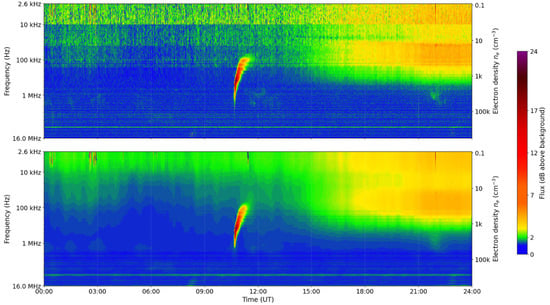
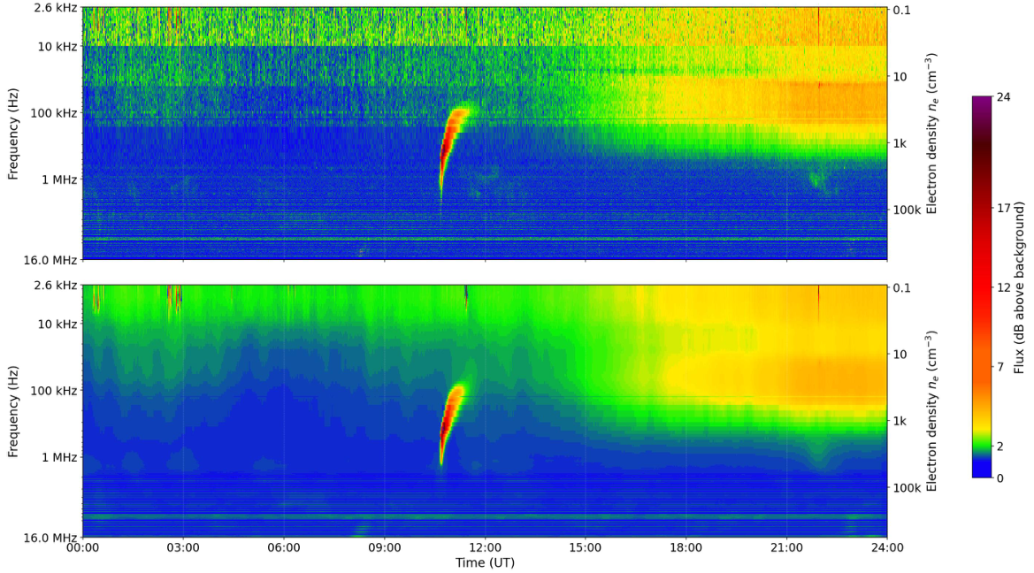
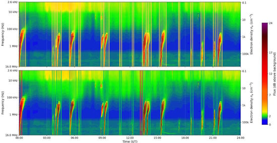
For denoising and background suppression, we employ the non-local means (NL-Means) [27] to enhance the normalized spectrograms. NL-Means exploits non-local self-similarity within the image; it reconstructs pixel intensities by computing a weighted average of similar patches found within a search window. While effectively suppressing random Gaussian noise, this method preserves the edge structures and texture details of radio bursts, thereby significantly improving the signal-to-noise ratio of weak events. In our pipeline, the spectrogram is first clipped to the operational range dB and linearly mapped to 8-bit before denoising; we then apply OpenCV’s fastNlMeansDenoising with a filter strength h = 10.0, a template patch and a search window (all sizes in pixels and required to be odd), and finally restore the pixel intensities to the original dB range. Figure 1 presents a visual comparison before and after denoising. The high-frequency noise and background fluctuations present in the original spectrogram are substantially suppressed after NL-Means processing. Conversely, the time–frequency boundaries of radio burst events become sharper, providing high-quality input representations for subsequent feature extraction and boundary regression.
Figure 1.
Visual comparison of denoising efficacy on a STEREO-A/SWAVES daily summary spectrogram (17 Aug 2021, DOY 229). The top panel displays the original spectrogram clipped to the operational dynamic range, while the bottom panel presents the result after processing with the NL-Means algorithm. The color bar encodes the radio flux in dB above the daily background level used by the SWAVES Level-3 product (range dB). The left vertical axis is the observation frequency on a logarithmic scale, spanning the full HFR–LFR range from ∼2.6 kHz at the top to ∼16 MHz at the bottom; the right vertical axis is the corresponding coronal/heliospheric electron density in cm−3, obtained from the fundamental plasma-frequency relation assuming fundamental plasma emission. The denoising process effectively suppresses background noise, thereby enhancing the clarity of texture structures and the sharpness of radio burst boundaries.
To prepare the final model input, we crop partial low-frequency channels (defaulting to indices below 37) and transpose the data to an format. Subsequently, the single-channel spectrogram is expanded into a three-channel tensor by replicating the channel dimension. It is then normalized using min-max scaling, yielding a tensor compatible with standard visual detection backbones.
3.3. Annotation Tool and Strategy
The detection framework is designed to regress temporal boundaries of Type III bursts, as their onset and duration serve as primary indicators for space weather alerting. Each event is annotated as a closed 1D time interval , with indices ranging from 0 to 1439 (corresponding to minute-resolution sampling over 24 h). Frequency-axis variation is preserved in input representations but not actively regressed during bounding box prediction. This annotation protocol implements the rationale summarized in Section 1: temporal endpoints are operationally primary, whereas frequency-wise box cuts would inject avoidable subjectivity and are less compatible with few-shot supervision, while the network still sees the full time–frequency context. To remain compatible with the standard Faster R-CNN training pipeline, each annotated interval is internally converted into a 2D bounding box that spans the full retained frequency extent of the input spectrogram, i.e., a degenerate-in-frequency box of the form in (time-min, freq-bin) coordinates. As a consequence, the conventional 2D IoU between such boxes reduces algebraically to the 1D temporal IoU defined in Section 5.3, ensuring that supervision and evaluation are strictly confined to the time axis. To facilitate the construction of a high-quality, reproducible training dataset, we developed X-Labeler2—an open-source, interactive annotation tool specifically designed for temporal interval labeling on solar radio dynamic spectra. X-Labeler enables users to drag-select event intervals along the time axis directly on spectrogram visualizations and export standardized label files in JSON format. This significantly streamlines the daily annotation workflow and supports efficient expert review of long-term observational records.
It should be noted that Type III bursts in the STEREO/SWAVES dataset are not always cleanly isolated from surrounding structures, as they may co-occur with Type II/IV continua, appear in temporally dense clusters, or be embedded in stripe interference and broadband noise. Under the single-class formulation adopted here, everything outside an annotated Type III interval is treated as background, including any co-occurring Type II/IV signal; intervals whose onset or end could not be reliably delineated, in particular dense Type III storms, were excluded from both training and evaluation, consistent with Section 6. The background distribution learned by the detector, therefore, contains a mixture of non-Type-III burst structures and rich noise patterns, which tends to tighten prototype matching against visually similar but physically distinct events. The year-by-year evaluation in Section 5.8 shows that precision remains stable at 83–88% across 2014–2023 despite large differences in burst clustering and noise level, suggesting that this imperfect isolation does not introduce a strong systematic bias.
4. Methodology
4.1. Framework Overview
We propose Meta-FSOD, a few-shot object detection framework grounded in episodic meta-learning. Each training episode is formulated as an N-way K-shot task with Q query samples per class, simulating the realistic constraint of learning from minimal labeled data. In this work, we configure episodes with N = 2 (foreground/background), K = 5 support set per class, and Q = 8 query set. The support set is used to compute class prototypes—compact representations derived from labeled examples—while the query set drives loss computation and parameter updates. This design explicitly trains the model to generalize from minimal supervision, enabling robust adaptation to novel event morphologies or domain shifts encountered during inference.
4.2. Feature Representation
We adopt ResNet [28] to facilitate the feature representation learning, leveraging its residual connections to mitigate gradient vanishing and facilitate optimization in deep networks. A residual block is formally defined as:
where x denotes the input feature map and represents a sequence of convolutional and non-linear transformations parameterized by W. Following He et al. [29], we employ preactivation and identity skip connections to ensure stable forward propagation and backward gradient flow.
To capture burst signatures across multiple scales—from narrowband drifting structures to broadband continua—we integrate Feature Pyramid Networks (FPNs) [24]. FPNs construct semantically rich, multi-resolution feature maps through top-down upsampling and lateral fusion:
where is the output of the l-th backbone layer, the corresponding pyramid feature, and denotes bilinear upsampling. This architecture bridges high-level semantics with low-level spatial details, enhancing representation capacity for diverse burst textures.
The detector is initialized with a Faster R-CNN (ResNet50-FPN backbone) pretrained on natural images [23,25]. Multi-scale features are extracted via the detector, and candidate region features are obtained using RoI Align. To facilitate metric learning, Meta-FSOD introduces a Prototype Projection Head, which maps RoI features into a 256-dimensional metric space followed by L2 normalization, ensuring feature alignment across different episodes.
4.3. Prototype-Based Recalibration
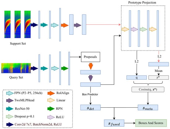
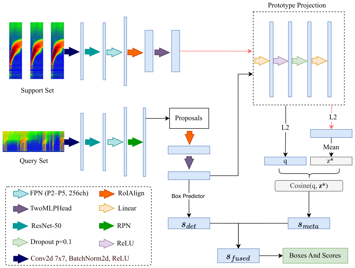
The core innovation of Meta-FSOD is the integration of support-set prototype learning with a metric recalibration mechanism. As illustrated in Figure 2, the framework extends the standard Faster R-CNN backbone with a dual-path inference scheme.
Figure 2.
Architecture of Meta-FSOD and the prototype recalibration process. The framework augments the baseline detector with a dual-path inference mechanism: the detector path outputs a classification score , while the prototype matching path computes a similarity score . The final score is derived via dynamic Beta Gating fusion. Distinct fill colors for the support and query spectrogram panels are used solely to visually separate the two subsets within an episode and do not convey additional physical or algorithmic meaning. In the schematic, denotes the L2-normalized embedding of a query RoI; the superscript asterisk is a diagrammatic label (not an operator) and denotes the same vector as z in the definition of immediately below.
During training, Meta-FSOD follows the episodic training paradigm. Each episode includes a support set and a query set. The support set consists of a few labeled samples (default k = 5), used to construct a prototype representation of the target class. The query set serves to evaluate generalization and guide parameter updates. For each image in the support set, features are first extracted using ResNet50-FPN, proposals are generated by the Region Proposal Network (RPN), and region features are pooled using RoI Align. These features are then projected into a 256-dimensional embedding space through the Prototype Projection Head and L2-normalized. The class prototype p—representing the radio burst category—is computed as the mean of all normalized positive RoI embeddings within the support set:
At inference, Meta-FSOD performs dual-path scoring for each candidate region in the query image. First, the query set is processed through the standard Faster R-CNN pipeline to yield detector confidence scores, denoted as . Simultaneously, the candidate RoI features of the query image are mapped to the embedding space and compared with the support-derived prototype p via cosine similarity, resulting in the metric score :
where z is the L2-normalized embedding of the query RoI.
To balance robustness and precision, we introduce a learnable gating mechanism:
where the gating weight is dynamically modulated by detector confidence:
where denotes the sigmoid function, is a confidence threshold, and is a learnable scaling factor. When , , causing the fused score to default to —thereby preventing the prototype branch from overreacting to low-confidence background regions. Conversely, when , approaches its maximum, allowing to refine high-confidence predictions through semantic alignment. This design functions as a precision-oriented false alarm suppressor: structured noise or radio frequency interference (RFI) may trigger high due to visual similarity, but typically exhibits low prototype matching (). The fusion mechanism downweights such spurious detections, significantly improving precision without sacrificing recall.
Given that solar Type III bursts frequently exhibit dense clustering and temporal overlap, traditional greedy Non-Maximum Suppression (NMS) risks erroneously discarding valid adjacent events. To address this, we employ the Soft-NMS strategy [26], which decays the scores of overlapping boxes using a Gaussian penalty rather than performing hard elimination:
where M is the current highest-scoring box, is an overlapping neighbor, and controls the decay rate. This preserves lower-scoring yet valid detections, ensuring they remain eligible for evaluation metrics such as mAP. As a result, recall in dense burst scenarios is substantially improved, reducing missed detections while maintaining ranking integrity.
Together, the dual-path scoring and Soft-NMS post-processing enable Meta-FSOD to leverage the generalization capacity of pretrained detectors while adapting rapidly to target-domain characteristics via few-shot support. This synergy yields significant gains in both precision and recall under annotation-scarce, real-world observational conditions.
4.4. Loss Function
The baseline FSOD model employs the standard Faster R-CNN loss [23], combining classification cross-entropy and Smooth L1 regression for bounding box localization. Meta-FSOD extends this objective by jointly optimizing detection performance and prototype alignment. The total loss, computed over the query set, is formulated as:
where denotes the standard detection loss and enforces metric consistency between query proposals and the foreground prototype derived from the support set. For each episode, a single foreground prototype is computed from RoIs of the support set:
where is the prototype projection head and is the set of positive RoIs in the support set. For each query example, we sample RPN proposals and keep positives/negatives by IoU (pos , neg ). Each selected proposal yields:
where is a fixed scale (default 10.0), equivalent to an inverse temperature. is passed through a sigmoid to produce a probability-like score . We then apply binary Focal Loss [30].
where is the set of all query RoIs in the episode, and is for positives. We set and . balances positives/negatives classes. This formulation encourages query regions that are semantically aligned with the burst prototype to receive high scores, while misaligned or background regions are suppressed.
5. Evaluation
5.1. Dataset
The experimental dataset is derived from one-minute-averaged HFR–LFR Level-3 dynamic spectra acquired by the STEREO-A/SWAVES. The data are organized daily, with each file represented as a matrix (frequency channels × temporal samples at minute resolution). To rigorously evaluate model generalization across different time periods, we adopted a cross-year validation strategy. The training set comprises observational data exclusively from 2024, consisting of 220 valid samples with 3377 annotated intervals. The test set, conversely, spans a broad historical period from 2014 to 2023, containing 1276 valid samples with 8941 annotated intervals. This partition ensures that training and testing are drawn from completely disjoint observation years, so that the cross-year stability of the model—i.e., whether detection performance remains consistent on data acquired in years that the model has never seen during training—can be assessed directly; the per-year breakdown is reported in Section 5.8.
5.2. Experimental Setup
All experiments were conducted on an NVIDIA RTX 4060 GPU (8 GB VRAM), using PyTorch 1.13 and CUDA 11.7.
The baseline FSOD model employs the Faster R-CNN architecture with a ResNet50-FPN backbone, initialized with COCO-pretrained weights [31]. To accommodate few-shot learning, we freeze the first three residual blocks (layer1–layer3) and fine-tune only layer4 and the detection head. Optimization is performed using AdamW, with learning rates of for the detection head and for the unfrozen backbone layers. Training spans 100 epochs with batch size 8.
Meta-FSOD extends this baseline by adding a 256-dimensional Prototype Projection Head, trained under an episodic meta-learning paradigm (K = 5, Q = 8). The prototype alignment loss weight is set to = 0.5, and the temperature scaling parameter as a learnable parameter is initialized to 1.0. Training proceeds in two stages: (1) 50 epochs optimizing only the prototype branch, followed by (2) 50 epochs of joint fine-tuning with the detector—stabilizing metric space learning.
5.3. Metrics
Performance evaluation is grounded in standard object detection protocols. We employ IoU as the quantitative measure of geometric alignment between predicted intervals (I) and ground truth (J). Given the 1D temporal nature of the task, IoU is computed strictly along the time axis:
where denotes the length of the time interval.
Based on a predefined IoU threshold (e.g., = 0.5), predictions are categorized as True Positives (TP), False Positives (FP), or False Negatives (FN). A prediction is considered a TP if its IoU with a ground truth interval exceeds . Conversely, predictions with IoU below , or those matching background regions, are classified as FP. Ground truth events missed by the model constitute FN.
From these counts, we derive the precision and recall:
Precision measures the reliability of positive predictions—critical for minimizing false alarms in operational systems. Recall quantifies coverage of true events—essential for scientific completeness. To provide a comprehensive assessment across varying confidence thresholds, we compute the average precision (AP)—defined as the area under the precision–recall (PR) curve—and report mAP as the primary performance metric.
5.4. Results
To quantitatively assess the effectiveness of the proposed framework, we first analyze the detection metrics of the Baseline and Meta-FSOD models. Table 1 and Table 2 detail the performance of the two approaches across varying confidence thresholds and IoU criteria, respectively.
Table 1.
Baseline (Faster R-CNN) performance on the test set (1276 samples, 8941 ground truth annotations).
Table 2.
Meta-FSOD ( support samples) performance on the test set (1276 samples, 8941 ground truth annotations).
At the practical operating point (IoU = 0.5, Confidence = 0.5), the Baseline model achieves a precision of 61.24% and a recall of 69.84%, yielding an mAP of 58.30%. However, it generates 3952 false positives (FP), indicating substantial noise sensitivity. In contrast, Meta-FSOD realizes a significant performance enhancement under identical conditions: precision rises to 81.46% (+20.22%), recall improves to 77.63% (+7.79%), and mAP increases to 73.30% (+15.00%). Notably, the FP count drops drastically to 1580, representing a 60.0% reduction.
In the loose setting oriented towards high recall (IoU = 0.1, Confidence = 0.2), the Baseline model attains a recall of 89.60% but suffers from a low precision of 40.05% and an excessive 11,990 false positives, which severely limits its operational utility. Conversely, Meta-FSOD maintains a comparable recall level (90.06%) while elevating precision to 64.51% (+24.5 pp) and reducing false positives to 4430 (a 63.1% reduction). These results demonstrate that Meta-FSOD effectively resolves the trade-off between high recall and low false-alarm rates, exhibiting superior false-alarm suppression capabilities.
Furthermore, we benchmark our approach against the traditional supervised method. Table 3 compares the experimental results of the Baseline, Meta-FSOD, and the YOLO-based model proposed by Scully et al. [14]. It is crucial to note the disparity in data scale: Scully et al. [14] employed approximately 60,000 training labels (6732 images), whereas this work utilized only 3377 labels (220 images)—an 18-fold difference. Despite this constraint, Meta-FSOD significantly outperforms the Baseline and the YOLO-based model. Although Meta-FSOD’s mAP of 73.30% is marginally lower than the 73.79% achieved by the YOLO-based model, under the looser IoU = 0.1 threshold, Meta-FSOD attains an mAP of 81.13%, outperforming the comparative methods. This indicates that even under extreme few-shot conditions, Meta-FSOD effectively leverages support-set information to suppress false positives while maintaining high recall, delivering performance that is superior to the baseline and competitive with large-data supervised approaches.
Table 3.
Performance comparison of Baseline, YOLO-based model (Scully), and our Meta-FSOD approach.
We deliberately restrict our quantitative benchmark to in-modality methods, because automatic detectors of other space-weather-relevant features (e.g., flares in EUV/SXR imagery, CMEs in coronagraph data, filament eruptions) differ from this work in target definition, labeling convention, evaluation metric (typically per-pixel or per-event F1 rather than IoU-based mAP), and supervision regime, so a direct numerical cross-comparison would be misleading. Within solar radio burst detection itself, the most relevant baseline is the fully supervised YOLO-based detector of Scully et al. [14] reported in Table 3: although trained on only 3377 labels (220 images), i.e., roughly 1/18 of Scully’s ∼60,000 labels (6732 images), Meta-FSOD attains comparable mAP@0.5 (73.30% vs. 73.79%) and clearly superior mAP@0.1 (81.13% vs. 74.78%, pp) while consistently leading on precision at every operating point shown (e.g., 81.46% vs. 64.74% at IoU/Conf = 0.5/0.5, pp; 64.51% vs. 40.11% at IoU/Conf = 0.1/0.2, pp). This indicates that, within the same modality, our few-shot framework is competitive with—and on the looser, recall-oriented operating points outperforms—the state-of-the-art fully supervised approach, while requiring an order of magnitude fewer annotations.
5.5. Visual Validation
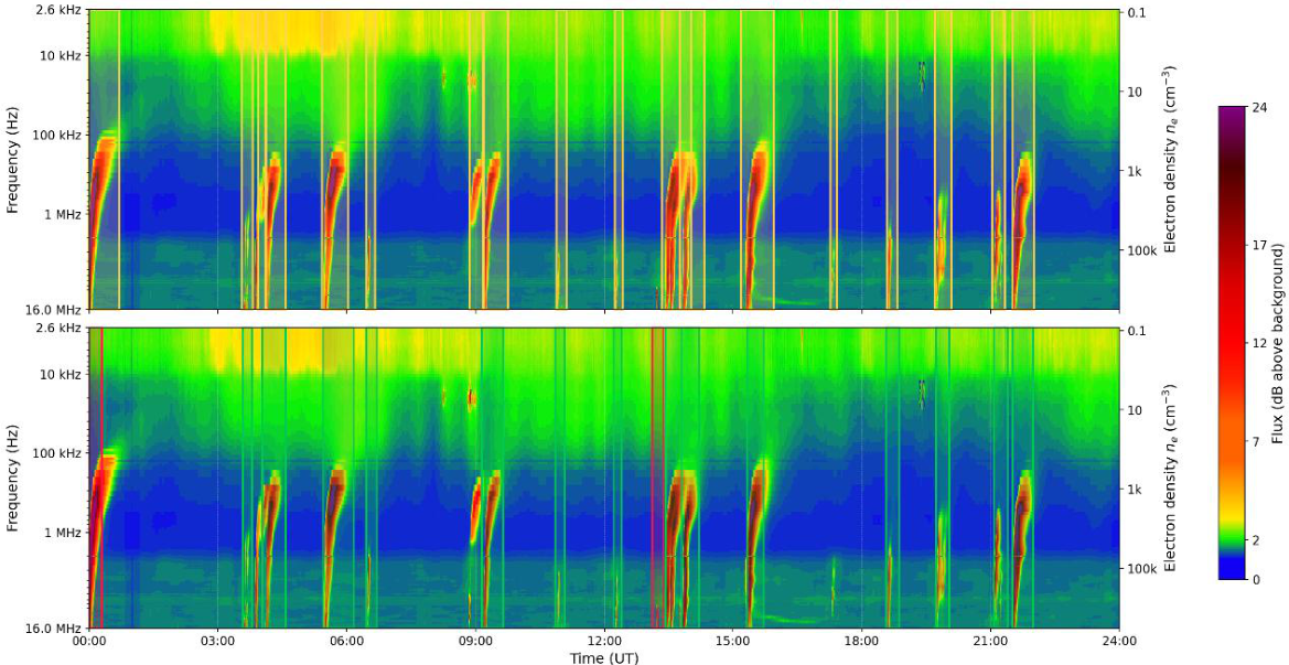
To complement the quantitative performance analysis, we present a visual assessment of the model’s detection capabilities. Figure 3 presents a representative day on which the test set covers a range of observational situations encountered during routine operation, from isolated bursts to temporally dense clusters and spectrally noisy backgrounds; we emphasize that these are qualitative descriptions of the day’s content rather than separately labeled categories, since this work formulates detection as a single-class problem (Type III vs. background) and any non-Type-III structure (e.g., stripe interference, broadband noise, low-amplitude signals) is treated as background by construction.
Figure 3.
Visualization of Meta-FSOD detection results on a representative test-set spectrogram. (Top panel): human-labeled ground truth, in which yellow boxes mark the Type III intervals annotated; everything outside these boxes (including any stripe interference, broadband noise, low-amplitude signals, or co-occurring non-Type-III structures) is treated as background under our single-class formulation. (Bottom panel): model predictions evaluated against the top panel, with green boxes denoting True Positives (predictions whose temporal IoU with a human-labeled interval is ≥0.5) and red boxes denoting False Positives (predictions whose temporal IoU is <0.5). Ground truth is, therefore, shown only in the top panel as yellow boxes; the color-mapping in the bottom panel is the standard TP/FP convention.
For isolated bursts, predicted intervals exhibit strong alignment with ground-truth annotations, demonstrating accurate temporal boundary regression. In dense scenarios—characterized by overlapping or continuous Type III bursts—Meta-FSOD successfully resolves individual events without merging or fragmentation, preserving event-level granularity. Under adverse background conditions, including instrument stripe artifacts, broadband noise, or low-amplitude signals, the prototype recalibration mechanism effectively suppresses spurious detections by verifying semantic consistency with support-set prototypes—functioning as a domain-adaptive confidence modulator rather than a heuristic “secondary confirmation”.
5.6. Ablation Study
To verify the individual contributions of the core components within Meta-FSOD, we conducted a stepwise ablation analysis on the test set. Table 4 details the results, using a configuration that includes only prototype recalibration (without Beta Gating or Soft-NMS) as the reference baseline (denoted as “Baseline (Proto)”).
Table 4.
Ablation study under IoU = 0.5, Confidence = 0.5, k = 5.
The results demonstrate the distinct benefits of each module. The introduction of Beta Gating has a suppression effect on false positives (FPs): precision improves from 79.45% to 80.16%, and the number of FPs is reduced from 1808 to 1723. This confirms the efficacy of dynamically modulating prototype influence based on detector confidence.
Incorporating Soft-NMS further refines performance. When applied alone, Soft-NMS increases precision to 80.97% and reduces FP to 1637. By decaying the scores of overlapping candidate boxes rather than eliminating them outright, Soft-NMS optimizes the scoring distribution. This allows high-scoring candidates that might have been erroneously discarded by standard NMS to be retained, thereby helping to preserve recall while filtering weak detections.
Finally, the Full Method, which integrates both Beta Gating and Soft-NMS, achieves the optimal trade-off. It attains the highest precision of 81.46% and minimizes FP to 1580 (a 12.6% reduction compared to the baseline), while maintaining a robust recall rate of 77.63%. These findings validate that the synergistic combination of dynamic gating and soft suppression mechanisms is crucial for maximizing detection purity without sacrificing event coverage.
5.7. Sensitivity to Support Set Size
As a few-shot learning method, the stability of model performance under different support set sizes k is a key indicator. To evaluate this, we assessed the detection performance of Meta-FSOD with k set to 1, 3, 5, and 10, as detailed in Table 5.
Table 5.
Performance comparison under different support set sizes k (IoU = 0.5, Confidence = 0.5).
The experimental results reveal two important trends:
1. Robustness under extreme scarcity: The model exhibits remarkable stability even in the extreme one-shot (K = 1) regime, achieving an mAP of 73.55% and a precision of 80.97%. This demonstrates that Meta-FSOD can construct a generalizable metric space using a single support example, effectively overcoming the dependency on extensive annotations characteristic of traditional deep learning methods.
2. Inverse correlation between support set size and FP: As K increases from 1 to 10, the number of FP consistently declines from 1637 to 1572. This trend suggests that a richer support set yields more robust and compact class prototypes, which are better equipped to reject ambiguous background noise. Although this improved specificity incurs a marginal reduction in recall (from 77.91% to 77.59%), trading a negligible loss in sensitivity for a significant reduction in false alarms is highly advantageous for bandwidth-constrained deep space missions.
Balancing annotation cost against detection performance, we adopt K = 5 as the default configuration for this work. This setting ensures a minimal annotation burden while delivering excellent control over FP.
The near-insensitivity of mAP to K is a direct consequence of the way the prototype is constructed: every support RoI feature is L2-normalized before being averaged, and the resulting prototype is L2-normalized again, so each additional support example mainly denoises the prototype direction in the embedding space rather than redefining it. Quantitatively, going from K = 1 to K = 10 moves mAP by only pp and reduces FP by about at the cost of pp recall. In practice, this means that the detector can be retargeted to a new instrument or observing epoch with as few as one to three expert-labeled support events without measurable mAP loss, which is operationally important for missions where each annotated burst is expensive to obtain.
5.8. Temporal Stability
To rigorously evaluate the model’s generalization in long-term observations, we conducted a per-year independent evaluation spanning from 2014 to 2023. Table 6 details the annual performance metrics.
Table 6.
Year-wise performance evaluation from 2014 to 2023 (IoU = 0.5, Confidence = 0.5).
The experimental results highlight the model’s robustness across varying levels of solar activity. In the active years (2021–2023) temporally proximate to the training data (2024), the model exhibits optimal comprehensive performance: mAP ranges between 71.74% and 81.17%, with recall peaking at 86.02% in 2023. This confirms the model’s exceptional detection capability within domains that approximate the training distribution.
Conversely, during Solar Cycle 24 (2014–2016), recall declined to approximately 64–69%, while precision remained consistently high (83–85%). We attribute this asymmetry to the temporal distance between these test years and the training epoch (2024): being roughly a decade apart, the 2014–2016 spectrograms differ from the training data in background level, stripe-artifact statistics, and the morphological mix of bursts (Solar Cycle 24 vs. Cycle 25), so a fraction of weaker or atypical events fall below the prototype-matching threshold and are missed. This is not a monotonic “instrument aging” effect—the more recent years 2017–2023, which are temporally closer to 2024, do not exhibit comparable recall degradation. The fact that precision remains high under this temporal distance indicates that Meta-FSOD continues to reject ambiguous background noise via strict prototype matching, trading some sensitivity for very few false alarms in years far from the training epoch.
Furthermore, during the solar minimum (2018–2020), when burst events were relatively sparse, the model not only maintained high detection precision (mAP 70.52–84.36%) but also minimized FP to an extremely low level. This evidences the model’s high reliability in quiescent background conditions.
6. Conclusions
Empirical results confirm that Meta-FSOD effectively addresses the challenge of annotation scarcity in solar radio Type III burst detection. Despite training on a dataset only 1/18th the size of comparable studies [14], our framework achieves an mAP of 73.30%, closely approaching the performance of large-scale trained models. Crucially, the synergistic integration of prototype recalibration and gating fusion mechanisms reduces FP while boosting precision at practical operating thresholds. Furthermore, rigorous cross-temporal validation (training on 2024 data, testing on 2014–2023) demonstrates the model’s robust generalization against solar cycle variations.
Beyond the algorithmic contribution, the framework lends itself to several concrete scientific and operational use cases. (i) As an on-board event-trigger for deep-space radio receivers (e.g., STEREO/SWAVES and future heliospheric or lunar far-side missions), it can flag burst-containing time windows so that only scientifically relevant segments are transmitted at full resolution under tight downlink budgets. (ii) As an automated cataloging tool for long-term archives, it can produce uniform Type III burst lists across many years with the same detector configuration, enabling statistical studies of occurrence rates, clustering, and burst duration as functions of solar cycle phase. (iii) As a prescreening component in space-weather pipelines, the high-precision operating point (∼81% precision, ∼78% recall at IoU = 0.5) provides a reliable, low-false-alarm input to downstream analyses such as solar energetic particle event association, where groups of intense Type III bursts often precede impulsive electron events. The annotation efficiency of the few-shot setting is particularly valuable in these settings, because the same architecture can be retargeted to a new instrument or epoch with only a handful of expert-labeled support events.
Nevertheless, several limitations remain. First, certain complex phenomena, such as dense or continuous Type III storms, were intentionally excluded from this study due to their inherently ambiguous temporal boundaries, which even expert annotators cannot consistently delineate, rendering reliable ground-truth labeling impractical. Second, while few-shot learning alleviates dependence on large-scale annotations, constructing high-quality support sets still requires curated input from domain experts, limiting full automation. Third, the detection of extremely weak events, whose signal-to-noise ratios approach background levels, remains challenging under high-confidence operating thresholds, where the model prioritizes precision over sensitivity.
Future research will focus on integrating unsupervised domain adaptation to leverage massive unlabeled data for cross-mission alignment. We also aim to enhance interpretability through attention visualization tools and to explore model compression techniques—such as knowledge distillation and quantization—to facilitate the deployment of lightweight detectors on embedded spaceflight hardware. A natural further extension is to other burst types (Type II and Type IV). The Meta-FSOD architecture is class-agnostic by construction—in principle, replacing the support set with Type II or Type IV examples is sufficient to retarget the detector—but two adaptations would be required for a rigorous study: (i) the supervision and evaluation should be lifted from a 1D temporal interval to a 2D time–frequency box, since Type II bursts are characterized by their slow frequency drift bands and Type IV continua by their bandwidth, both of which are scientifically meaningful and not easily reduced to onset/end times; and (ii) the single-prototype, dual-path scoring must be generalized to a multi-class formulation (one prototype per burst type, plus an explicit background contrast), so that visually similar but physically distinct bursts can be discriminated rather than collapsed onto a single foreground category. We leave the construction of a multi-class support set spanning Types II/III/IV across STEREO/SWAVES and complementary ground-based instruments to follow-up work.
Author Contributions
Conceptualization, H.J. and S.W.; methodology, H.J.; software, L.C.; validation, B.L., W.D., and Z.Z.; formal analysis, H.J.; investigation, L.C.; resources, Z.Z.; data curation, B.L.; writing—original draft preparation, H.J.; writing—review and editing, S.W.; visualization, L.C.; supervision, S.W.; project administration, H.Z.; funding acquisition, S.W. All authors have read and agreed to the published version of the manuscript.
Funding
This research was funded by the National Key Research and Development Program of China (Grant No. 2022YFF0503801), the National Natural Science Foundation of China (Grants No. 62462041), and the China Manned Space Program (Grant No. CMS-CSST-2025-A19).
Data Availability Statement
The dataset for training and evaluation in this research is from the STEREO-A/SWAVES (https://stereo.space.umn.edu/data/level-3/STEREO/Ahead/SWAVES/one-minute/IDL/HFR-LFR/ (accessed on 6 December 2025)).
Acknowledgments
We are sincerely grateful to the anonymous reviewers for their insightful comments and constructive suggestions, which have significantly improved the clarity and quality of this manuscript. We also thank our colleagues at the Computer Technology Application Key Lab of Yunnan Province for their stimulating discussions and technical support throughout this research. Special appreciation goes to Xiaoli Zhang for assistance with the experimental setup and data analysis. Finally, we acknowledge the editorial team for their efficient handling of our submission.
Conflicts of Interest
The authors declare no conflicts of interest.
Notes
| 1 | https://stereo.space.umn.edu/data/level-3/STEREO/Ahead/SWAVES/one-minute/IDL/HFR-LFR/ (accessed on 6 December 2025). |
| 2 | https://github.com/kustcn/x-labeler (accessed on 31 October 2025). |
References
- Camporeale, E. The Challenge of Machine Learning in Space Weather: Nowcasting and Forecasting. Space Weather 2019, 17, 1166–1207. [Google Scholar] [CrossRef] [Scilit]
- Reid, H.A.S.; Ratcliffe, H. A Review of Solar Type III Radio Bursts. Res. Astron. Astrophys. 2014, 14, 773–804. [Google Scholar] [CrossRef] [Scilit]
- Nindos, A.; Aurass, H.; Klein, K.L.; Trottet, G. Radio Emission of Flares and Coronal Mass Ejections. Sol. Phys. 2008, 253, 3–41. [Google Scholar] [CrossRef] [Scilit]
- Benz, A.O. Flare Observations. Living Rev. Sol. Phys. 2017, 14, 2. [Google Scholar] [CrossRef] [Scilit]
- Li, T.M.; Li, C.; Chen, P.F.; Ding, W.J. Particle-in-cell Simulation of Plasma Emission in Solar Radio Bursts. Astron. Astrophys. 2021, 653, A169. [Google Scholar] [CrossRef] [Scilit]
- Bougeret, J.L.; Goetz, K.; Kaiser, M.L.; Bale, S.D.; Kellogg, P.J.; Maksimovic, M.; Monge, N.; Monson, S.J.; Astier, P.L.; Davy, S.; et al. S/WAVES: The Radio and Plasma Wave Investigation on the STEREO Mission. Space Sci. Rev. 2008, 136, 487–528. [Google Scholar] [CrossRef] [Scilit]
- Benz, A.O.; Monstein, C.; Meyer, H.; Manoharan, P.K.; Ramesh, R.; Altyntsev, A.; Lara, A.; Paez, J.; Cho, K.S. A World-Wide Net of Solar Radio Spectrometers: e-CALLISTO. Earth Moon Planets 2009, 104, 277–285. [Google Scholar] [CrossRef] [Scilit]
- van Haarlem, M.P.; Wise, M.W.; Gunst, A.W.; Heald, G.; McKean, J.P.; Hessels, J.W.; de Bruyn, A.G.; Nijboer, R.; Swinbank, J.; Fallows, R.; et al. LOFAR: The LOw-Frequency ARray. Astron. Astrophys. 2013, 556, A2. [Google Scholar] [CrossRef] [Scilit]
- Huang, J.; Tan, B. Radio Spectrum Observations and Studies of the Solar Broadband Radio Dynamic Spectrometer (SBRS). Universe 2024, 10, 440. [Google Scholar] [CrossRef] [Scilit]
- Hamini, A.; Auxepaules, G.; Birée, L.; Kenfack, G.; Kerdraon, A.; Klein, K.L.; Lespagnol, P.; Masson, S.; Coutouly, L.; Fabrice, C.; et al. ORFEES—A Radio Spectrograph for the Study of Solar Radio Bursts and Space Weather Applications. J. Space Weather Space Clim. 2021, 11, 57. [Google Scholar] [CrossRef] [Scilit]
- Lobzin, V.V.; Cairns, I.H.; Zaslavsky, A. Automatic Recognition of Type III Solar Radio Bursts in STEREO/WAVES Data for Onboard Real-Time and Archived Data Processing. J. Geophys. Res. Space Phys. 2014, 119, 742–750. [Google Scholar] [CrossRef] [Scilit]
- Salmane, H.; Weber, R.; Abed-Meraim, K.; Klein, K.L.; Bonnin, X. A Method for the Automated Detection of Solar Radio Bursts in Dynamic Spectra. J. Space Weather Space Clim. 2018, 8, A43. [Google Scholar] [CrossRef] [Scilit]
- Zhang, W.; Wang, B.; Wu, Z.; Chen, Y.; Yan, F. Identification and Extraction of Type II and III Radio Bursts Based on YOLOv7. Astron. Astrophys. 2024, 683, A51. [Google Scholar] [CrossRef] [Scilit]
- Scully, J.; Flynn, R.; Gallagher, P.T.; Carley, E.P.; Daly, M. Improved Type III Solar Radio Burst Detection Using Congruent Deep Learning Models. Astron. Astrophys. 2023, 674, A218. [Google Scholar] [CrossRef] [Scilit]
- Guo, J.C.; Yan, F.B.; Wan, G.; Hu, X.J.; Wang, S. A Deep Learning Method for the Recognition of Solar Radio Burst Spectrum. PeerJ Comput. Sci. 2022, 8, e855. [Google Scholar] [CrossRef] [Scilit]
- Murphy, P.C.; Cecconi, B.; Briand, C.; Aicardi, S. Automatic Detection of Solar Radio Bursts in NenuFAR Observations. arXiv 2024, arXiv:2401.04469. [Google Scholar] [CrossRef] [Scilit]
- Bussons Gordo, J.; Fernández Ruiz, M.; Prieto Mateo, M.; Alvarado Díaz, J.; Chávez de la, O.F.; Ignacio Hidalgo, J.; Monstein, C. Automatic Burst Detection in Solar Radio Spectrograms Using Deep Learning: deARCE Method. Sol. Phys. 2023, 298, 82. [Google Scholar] [CrossRef] [Scilit]
- Wang, Y.; Li, X.; Huang, J.; Zhou, Z.; Zhang, Z. A Survey of Few-Shot Learning. J. Softw. 2021, 32, 349–369. (In Chinese) [Google Scholar] [CrossRef]
- Snell, J.; Swersky, K.; Zemel, R. Prototypical Networks for Few-Shot Learning. In Advances in Neural Information Processing Systems, Proceedings of the 31st Conference on Neural Information Processing Systems (NIPS 2017), Long Beach, CA, USA; Curran Associates, Inc.: Red Hook, NY, USA, 2017; Volume 30. [Google Scholar]
- Vinyals, O.; Blundell, C.; Lillicrap, T.; Kavukcuoglu, K.; Wierstra, D. Matching Networks for One Shot Learning. In Advances in Neural Information Processing Systems, Proceedings of the 30th Conference on Neural Information Processing Systems (NIPS 2016), Barcelona, Spain; Curran Associates, Inc.: Red Hook, NY, USA, 2016. [Google Scholar]
- Kang, M.; Ege, M.; Gross, H.M. Few-Shot Object Detection: A Comprehensive Survey. IEEE Trans. Neural Netw. Learn. Syst. 2023, 35, 11958–11978. [Google Scholar] [CrossRef] [Scilit]
- Yan, X.; Chen, Z.; Xu, A.; Wang, X.; Liang, X.; Lin, L. Meta R-CNN: Towards General Solver for Instance-Level Low-Shot Learning. In Proceedings of the IEEE/CVF International Conference on Computer Vision (ICCV); IEEE: New York, NY, USA, 2019; pp. 9577–9586. [Google Scholar] [CrossRef] [Scilit]
- Ren, S.; He, K.; Girshick, R.; Sun, J. Faster R-CNN: Towards Real-Time Object Detection with Region Proposal Networks. In Advances in Neural Information Processing Systems; Curran Associates, Inc.: Red Hook, NY, USA, 2015; Volume 28, pp. 91–99. [Google Scholar] [CrossRef] [Scilit]
- Lin, T.Y.; Dollár, P.; Girshick, R.; He, K.; Hariharan, B.; Belongie, S. Feature Pyramid Networks for Object Detection. In Proceedings of the IEEE Conference on Computer Vision and Pattern Recognition (CVPR); IEEE: New York, NY, USA, 2017; pp. 2117–2125. [Google Scholar] [CrossRef] [Scilit]
- Farias, H.; Damke, G.; Solar, M.; Jaque Arancibia, M. Accelerated and Energy-Efficient Galaxy Detection: Integrating Deep Learning with Tensor Methods for Astronomical Imaging. Universe 2025, 11, 73. [Google Scholar] [CrossRef] [Scilit]
- Bodla, N.; Singh, B.; Chellappa, R.; Davis, L.S. Soft-NMS—Improving Object Detection with One Line of Code. In Proceedings of the IEEE International Conference on Computer Vision (ICCV); IEEE: New York, NY, USA, 2017; pp. 5561–5569. [Google Scholar] [CrossRef] [Scilit]
- Buades, A.; Coll, B.; Morel, J.M. Non-local means denoising. Image Process. Line 2011, 1, 208–212. [Google Scholar] [CrossRef] [Scilit]
- He, K.; Zhang, X.; Ren, S.; Sun, J. Deep Residual Learning for Image Recognition. In Proceedings of the IEEE Conference on Computer Vision and Pattern Recognition (CVPR); IEEE: New York, NY, USA, 2016; pp. 770–778. [Google Scholar] [CrossRef] [Scilit]
- He, K.; Zhang, X.; Ren, S.; Sun, J. Identity Mappings in Deep Residual Networks. In Computer Vision—ECCV 2016. ECCV 2016; Springer: Cham, Switzerland, 2016; pp. 630–645. [Google Scholar] [CrossRef] [Scilit]
- Lin, T.Y.; Goyal, P.; Girshick, R.; He, K.; Dollár, P. Focal Loss for Dense Object Detection. In Proceedings of the IEEE International Conference on Computer Vision (ICCV); IEEE: New York, NY, USA, 2017; pp. 2980–2988. [Google Scholar] [CrossRef] [Scilit]
- Li, W. Analysis of Object Detection Performance Based on Faster R-CNN. J. Phys. Conf. Ser. 2021, 1827, 012085. [Google Scholar] [CrossRef] [Scilit]

Disclaimer/Publisher’s Note: The statements, opinions and data contained in all publications are solely those of the individual author(s) and contributor(s) and not of MDPI and/or the editor(s). MDPI and/or the editor(s) disclaim responsibility for any injury to people or property resulting from any ideas, methods, instructions or products referred to in the content. |
© 2026 by the authors. Licensee MDPI, Basel, Switzerland. This article is an open access article distributed under the terms and conditions of the Creative Commons Attribution (CC BY) license.