Numerical Tools for Electroweak Phase Transition

Abstract

The electroweak phase transition serves as a crucial portal to explore physics beyond the Standard Model, with profound implications for gravitational waves, baryogenesis, dark matter, and vacuum stability. We review the computational workflow for analyzing cosmological phase transitions, which includes constructing the finite-temperature effective potential, identifying possible phases, tracing transition history, calculating transition rates, milestone temperatures, and thermal parameters, as well as the numerical tools developed for each step. We compare the functionalities, strategies, and applicable scopes of these tools, aiming to provide a practical guide that helps researchers select the most appropriate computational resources for their studies.

1. Introduction

The Standard Model (SM) of particle physics, while remarkably successful, leaves several fundamental questions unanswered, including the nature of dark matter (DM), the origin of the observed baryon asymmetry of the universe, and the dynamics of cosmic inflation [1,2,3,4,5]. These mysteries strongly suggest the existence of physics beyond the Standard Model (BSM). Since direct searches for new particles at the Large Hadron Collider (LHC) have not yet produced strong evidence [5,6,7,8,9,10,11,12], a variety of alternative approaches are gaining traction.

The discovery of gravitational waves [13,14] opens a new avenue for exploring BSM. The operational ground-based interferometer [15,16,17], the pulsar timing arrays [18,19,20,21], the upcoming space-based interferometers [22,23,24] and various tabletop experiments [25,26] cover gravitational wave signals across different frequency bands. In BSM, one of the most motivated sources of gravitational waves are electroweak first-order phase transitions (EWPT) in the early universe [27,28,29,30]. In such an epoch, the Universe decays from a symmetric, high-temperature phase into the Higgs-broken vacuum, low-temperature phase and forms bubbles spontaneously in the thermal plasma. With the expansion of bubbles, they collide and merge with each other and convert the whole spacetime into the stable vacuum. The collision of bubble walls, the subsequent sound waves, and magnetohydrodynamic turbulence act as sources of gravitational radiation, leading to a stochastic GW background. Within the SM framework, the EWPT is typically a smooth crossover [31], lacking significant observational consequences. However, numerous BSM scenarios, such as those with extended Higgs sectors or new scalar fields, can profoundly alter the nature of this transition, making it a strong first-order phase transition (FOPT) [32,33,34,35,36,37].

Moreover, a strong FOPT is a prerequisite for electroweak baryogenesis, a compelling mechanism to explain the matter-antimatter asymmetry [38,39]. The properties of the phase transition are also intimately linked to questions of vacuum stability [40,41,42,43] and can influence the production mechanism for dark matter [44,45,46,47,48,49,50,51,52,53]. Consequently, the study of the EWPT provides a powerful and complementary pathway to BSM physics, connecting particle theory to cosmic physics.

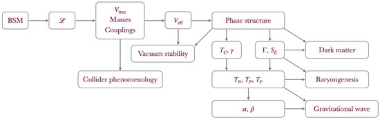
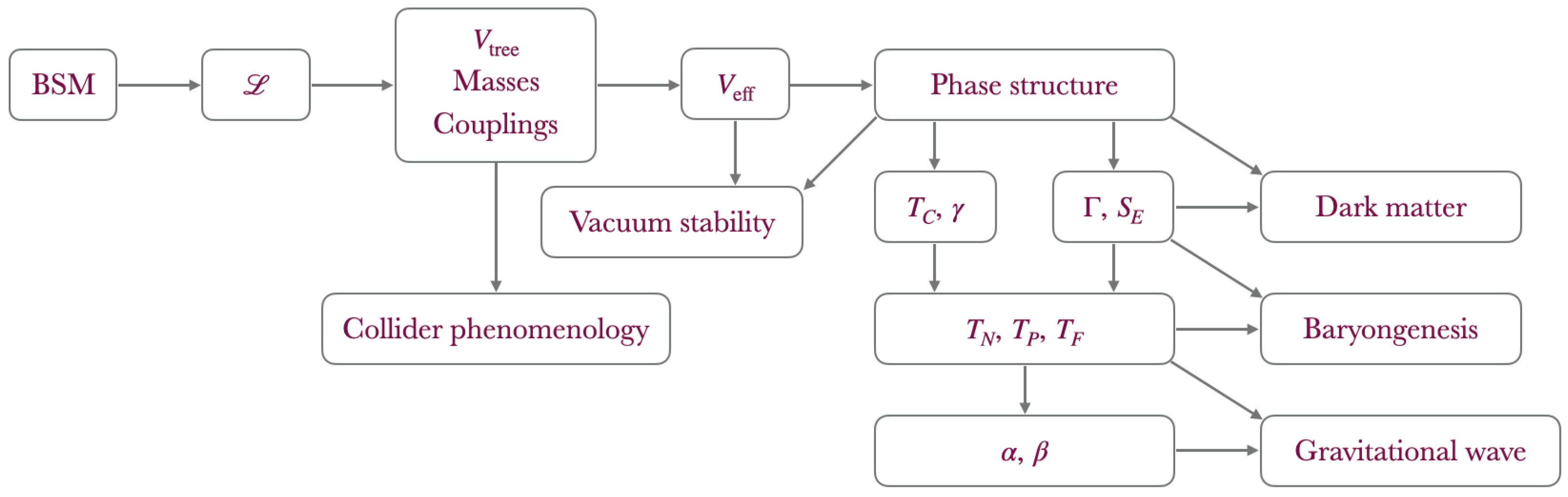
Figure 1 shows the pathway for investigating phase transitions in BSM models. It begins with the Lagrangian of specific physics model, proceeds to calculate the tree-level scalar potential $V_{\mathrm{tree}}$, field-dependent masses, thermal corrections and then constructs the finite-temperature effective potential $V_{\mathrm{eff}}$. This potential, which is a function of the classical fields, serves as the foundational input. The first analytical step is to identify all minimums of the effective potential across a range of temperatures to map out all possible phases. The core task then is to determine the possible phase transitions between these phases, particularly FOPT. The critical temperature $T_C$ (at which the two phases have degenerate potential) and the order parameter $\gamma$ are straightforward to compute. However, determining additional milestone temperatures and corresponding phase transition parameters is more involved. A key step is the calculation of transition rates per unit time $\Gamma$, which depends on evaluating the bounce action $S_E$ and requires solving a set of partial differential equations. Once the transition rates are obtained, one can proceed to compute the nucleation temperature $T_N$ (at which one bubble nucleates per Hubble volume), the percolation temperature $T_P$ (at which the bubbles form an connected network), and the completion temperature $T_F$ (at which the universe essentially completes the transition). Finally, at these characteristic temperatures, thermal parameters such as the transition strength $\alpha$, the inverse duration of the transition $\beta$, and the bubble-wall velocity $v_w$ can be evaluated. With all these phase-transition quantities determined, the results can be used for gravitational-wave prediction, baryogenesis, dark-matter studies, and vacuum-stability analyses.

Figure 1. The Workflow for performing a phase transition phenomenological study in BSM theories.

In recent years, various sophisticated software packages have been developed to streamline these calculations, mitigate the risk of manual errors, and enhance the reliability of results. This review aims to provide an overview the prevalent numerical tools dedicated to the study of the electroweak phase transition. We will focus on widely-used packages including CosmoTransitions_v2.0.6 [54], BSMPT_3.1.13 [55,56,57], PhaseTracer_2.2.0 [58,59], TransitionListener [60], PT2GWFinder_1.1.0 [61], ELENA [62], AnyBubble_2.0.4 [63], BubbleProfiler_1.0.1 [64], SimpleBounce_1.0 [65], FindBounce_1.2.0 [66], TransitionSolver [59], Vevacious_1.2.03 [67], thermal_funcs [68], DRalgo_1.3.0 [69], WallGo_1.1.1 [70,71], BubbleDet_1.0.7 [72], as well as an unnamed code [73]. This review seeks to serve as a practical guide for researchers in selecting the appropriate tools for their specific investigations.

In Table 1, we briefly list the key features of numerical tools for analyzing cosmological phase transitions, including CosmoTransitions, BSMPT, PhaseTracer, TransitionListener, PT2GWFinder, ELENA and TransitionSolver. Additionally, AnyBubble, BubbleProfiler, SimpleBounce, and FindBounce are designed to solve the bounce equations, compute the bounce action and the bubble profile. thermal_funcs can be used for calculating thermal functions. DRalgo and the codes in Ref. [73] are employed to calculate the bubble wall velocity. BubbleDet computes the prefactor in the transition rate. In the following sections, we will discuss these tools in detail.

Table 1. Key features of numerical tools for analyzing cosmological phase transitions.

Software	Effective Potential	Phase History	Bounce Action Calculation	${\mathit{T}}_{\mathit{N}}$ Formula Reference	${\mathit{T}}_{\mathit{P}}$ Support
CosmoTransitions	$\overline{\mathrm{MS}}$ scheme	Tracing	Path deformation	Equation (20)	No
BSMPT	Multi-Higgs models	Bisection (V1/V), Tracing (V3)	Path deformation	Equation (18)	Yes
PhaseTracer	Various renormalization schemes (Linkable to BSMPT, FlexibleSUSY)	Tracing	Path deformation Based on BubbleProfiler	Equation (20)	Yes
TransitionListener	Based on CosmoTransitions	Tracing	Based on CosmoTransitions	Equation (19)	No
PT2GWFinder	Linkable to Dralgo	Tracing	Based on FindBounce	All available choices	Yes
ELENA	Based on CosmoTransitions	Tracing	Tunneling potential formalism (single-field potentials)	Equation (17)	Yes

2. Effective Potential

The perturbatively calculated effective potential is built upon the tree-level classical potential, $V_0$, from the Lagrangian. Zero-temperature radiative corrections are then included via the sum of connected, loop level one-particle irreducible diagrams at zero external momentum. These corrections are notably dependent on the choice of gauge and renormalization scheme [74,75]. In the standard approach using the Landau gauge and $\overline{\mathrm{MS}}$ scheme, the one-loop contribution takes the form [74,76,77]:

$$V_1^{T=0}\left(\varphi \right)={\displaystyle \frac{1}{64{\pi }^2}}\sum _i{(-1)}^{2s_i}(1+2s_i)m_i^4\left(\varphi \right)\left[log\left({\displaystyle \frac{m_i^2\left(\varphi \right)}{{\mu }^2}}\right)-k_i\right]$$

(1)

where the sum extends over all degrees of freedom (real scalar, fermion and vector boson), $s_i$ denotes the spin of field i, and $k_i$ is $\frac{3}{2}$ for scalars and fermions and $\frac{6}{5}$ for gauge bosons. The background field is denoted by $\varphi$, $m_i\left(\varphi \right)$ are the field-dependent masses, and $\mu$ is the renormalization scale.

The finite-temperature corrections to the effective potential in the Landau gauge can be written in terms of the thermal function [77,78,79]

$$V_1^T\left(\varphi \right)={\displaystyle \frac{T^4}{2{\pi }^2}}\left[\sum _i{n}_{{\varphi }_i}{J}_B\left({\displaystyle \frac{m_{{\varphi }_i}^2}{T^2}}\right)+\sum _j{n}_{V_j}{J}_B\left({\displaystyle \frac{m_{V_j}^2}{T^2}}\right)-\sum _k{n}_{f_k}{J}_B\left({\displaystyle \frac{m_{f_k}^2}{T^2}}\right)\right],$$

(2)

where $n_{i,j,k}$ denote the degrees of freedom, taken as 1 for scalar fields, 3 for massive vector bosons, 2 for massless vector bosons, and 2 for fermion fields. The thermal function is defined as

$$J_{B/F}\left(y^2\right)={\int }_0^{\infty }\mathrm{d}k{k}^{2}log\left[1\mp e^{-\sqrt{k^2+y^2}}\right].$$

(3)

The finite-temperature perturbation theory breaks down at high temperatures. This issue can be addressed by resumming the leading infrared-divergent contributions, such as the Parwani method [80] and the Arnold–Espinosa method [81]. To this end, we need to obtain the temperature-corrected masses, namely the Debye masses. These masses are derived from the high-temperature expansion of finite-temperature self-energies for diagrams with zero Matsubara modes, in the limit of vanishing momenta. At the one-loop order within the Parwani framework, resummation is achieved by replacing the tree-level masses appearing in the $J_B$ functions with Debye masses for each contributing boson. The Arnold–Espinosa procedure replaces the mass parameters in the high-temperature expansion of the finite-temperature potential with thermal masses. An alternative approach to resolving infrared divergences is to integrate out the temperature dependence by matching to a three-dimensional effective field theory (3DEFT) [82,83]. The three-dimensional theory contains only zero Matsubara modes at the matching scale, and temperature dependence is introduced through the coupling determined by the matching conditions. This method yields higher precision and smaller uncertainties when the transition temperature is much larger than the relevant field scale [84,85,86].

The effective potential is the main input for most phase transition tools, though it is usually unnecessary to derive the full expression from scratch. Vevacious and DRalgo can automatically construct an effective potential. Vevacious is a tool designed for studying vacuum stability, not phase transitions, but both analyses are based on the same effective potential. It can import model files generated by the Mathematica [87] package SARAH [88]. Since the tool focuses on low-temperature physics, Daisy resummation [80,81] is not required. DRalgo is designed to automate the construction of 3DEFT for high-temperature phase transitions. It is done by specifying the gauge group, particle representations (scalars, fermions, gauge bosons), along with their respective charges and spinors. Based on these inputs, it then constructs the tree-level scalar potential and the Yukawa/fermion mass terms, and finally executes the dimensional reduction pipeline. PT2GWFinder offers an interface with DRalgo, by implementing the helper file DRTool to uses dimensionally-reduced potentials.

In CosmoTransitions, the formulas for one-loop zero-temperature contributions Equation (1), finite-temperature contributions Equation (2), and thermal functions Equation (3) are already implemented. Thus, users only need to input the expressions for the tree-level potential and field-dependent masses. By default, the infrared divergences at high temperature is not included, so it does not require the expressions of Debye masses. The thermal functions $J_{B/F}$ are calculated via direct numerical integration in the Python 3.11 library SciPy [89]. To speed up repeated evaluations, the results of direct integration are stored as a grid of precomputed values. Cubic interpolation is then used to quickly estimate the $J_{B/F}$. ELENA constructs the finite-temperature scalar potential using the model class in CosmoTransitions, and TransitionListener is built upon CosmoTransitions and extends its effective potential by incorporating contributions from daisy diagrams.

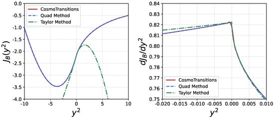
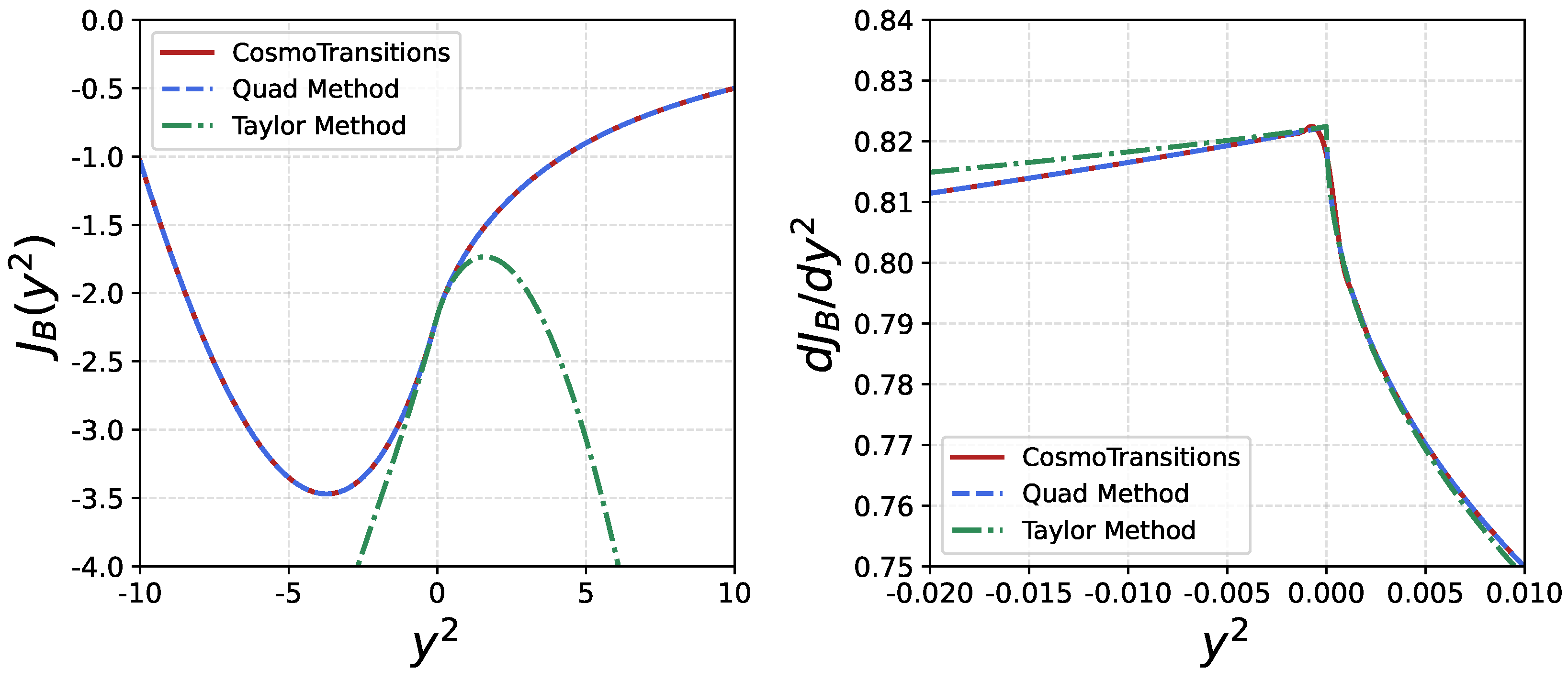
C++ library thermal_funcs [68,90] implements fast and accurate computations of thermal functions $J_{B/F}$ —along with their first and second derivatives with respect to $y^2$ in Equation (3). It supports six complementary numerical methods tailored to different ranges of $y^2$: numerical quadrature, Bessel function summation, Taylor expansion, asymptotic representations using Hurwitz zeta functions and polylogarithms, leading-order approximations, and asymptotic bounds. Figure 2 shows the function $J_B$ (left panel) and its derivative near $y^2$ (right panel), computed using different methods in thermal_funcs as well as in CosmoTransitions. The Quad method performs numerical quadrature, employing the QUADPACK [91] algorithms from the GNU Scientific Library to treat singularities in the integrand. The results are in agreement with the interpolation from CosmoTransitions over most of the region, except near $y^2=0$ where discrepancies in the derivative are observed. Thus, we also show the outcome of the Taylor expansion, which is accurate near $y^2=0$ but fails away from it. This comparison demonstrates that the results from the Quad method are more reliable. The error near $y^2=0$ can lead to wrong results in specific scenarios, such as the spurious identification of a minimum in the effective potential.

Figure 2. Thethermal function $J_B$ and its derivative calculated using CosmoTransitions (red line), as well as thermal_funcs with the Quad method (blue dash line) and the Taylor method (green dot line).

BSMPT is well-suited for multi-Higgs models and accepts input parameters from ScannerS [92]. It provides implementations of the CP-conserving 2-Higgs-Doublet Model (2HDM), the CP-violating 2HDM [56,93], and the Next-to-Minimal 2HDM [94]. Additionally, the code includes several analytically tractable potentials for validation, the CxSM and the example model from CosmoTransitions.

PhaseTracer offers a potential input mode similar to that of CosmoTransitions, but with an expanded set of features. It supports both the Parwani procedure and the Arnold–Espinosa procedure to handle infrared divergences at high temperature, the $\overline{\mathrm{MS}}$ scheme, on-shell-like schemes in $R_{\xi }$ gauge, and calculations in covariant gauge. The gauge-independent ℏ-expansion method [74,85,95,96,97,98,99,100] is also implemented. PhaseTracer can be linked to FlexibleSUSY [101] and BSMPT. The latest version provides several example models, including the two-dimensional test potential from CosmoTransitions, the dimensionally-reduced Abelian Higgs model implemented in DRalgo [69], the $Z_2$ scalar singlet model under various renormalization schemes [75], and the Left-Right symmetric model [102].

3. Phase History

Here a “phase” refers to a vacuum state corresponding to a local minimum of the finite-temperature effective potential. Once the potential is specified, the workflow includes finding its local minimums at different temperatures, categorizing these minimums into phases, and searching for possible phase transitions among the identified phases. This procedure will be explained in detail later with an explicit example.

For very simple potentials, such as the high-temperature approximation of models involving one or two scalar fields, the minima can be derived analytically. For example, for the SM extended with a $Z_2$-symmetric real scalar singlet (xSM), the high-temperature approximation is given by [103],

$$V({\varphi }_h,{\varphi }_s,T)={\displaystyle \frac{({\mu }_h^2+c_h{T}^2)}{2}}{\varphi }_h^2+{\displaystyle \frac{{\lambda }_h}{4}}{\varphi }_h^4+{\displaystyle \frac{{\lambda }_{hs}}{2}}{\varphi }_h^2{\varphi }_s^2+{\displaystyle \frac{({\mu }_s^2+c_s{T}^2)}{2}}{\varphi }_s^2+{\displaystyle \frac{{\lambda }_s}{4}}{\varphi }_s^4,$$

(4)

where ${\varphi }_h$ and ${\varphi }_s$ are the background field for the Higgs h and the extended real scalar singlet s, ${\mu }_h^2$ and ${\mu }_s^2$ are the coefficient of the quadratic term, ${\lambda }_h$ and ${\lambda }_s$ are the self-couplings, and ${\lambda }_{hs}$ is the portal coupling that connects the two sectors. $c_h$ and $c_s$ are thermal correction coefficients, arising from contributions of gauge bosons and fermions to the effective potential. There are three extrema,

$$(h_0,s_0)=(0,0),(h_1,s_1)=(\sqrt{-{\displaystyle \frac{{\mu }_h^2+c_h{T}^2}{{\lambda }_h}}},0),(h_2,s_2)=(0,\sqrt{-{\displaystyle \frac{{\mu }_s^2+c_s{T}^2}{{\lambda }_s}}}).$$

(5)

Substituting them back into Equation (4), we can obtain the potentials corresponding to these minimums, thereby deriving the critical temperature $T_C$ at which

$$V(h_1,s_1,T_C)=V(h_2,s_2,T_C).$$

(6)

The physical meaning of $T_C$ will be specified later. Here it is given by

$$T_C^2={\displaystyle \frac{{\lambda }_h{c}_s{\mu }_s^2-{\lambda }_s{c}_h{\mu }_h^2-\sqrt{{\lambda }_h{\lambda }_s}|c_s{\mu }_h^2-c_h{\mu }_s^2|}{{\lambda }_s{c}_h^2-{\lambda }_h{c}_s^2}}$$

(7)

This analytical approach is restricted to potentials of simple form. There are some examples of simple potential in BSMPT v3.

For potentials incorporating full loop corrections, obtaining the minimums analytically becomes infeasible, necessitating the use of numerical methods. BSMPT v1 uses a bisection method for calculating $T_C$, which is efficient and robust if there is only a single transition between two phases. Figure 3 demonstrates the iterative bisection procedure for locating $T_C$. The algorithm operates on a temperature interval $[T_{\mathrm{Low}},T_{\mathrm{High}}]$ that is guaranteed to contain $T_C$. By iteratively evaluating the global minimum at the midpoint $T_{\mathrm{Mean}}$ and updating the interval bounds based on its location (relative to the origin), the search range is systematically refined until it converges to $T_C$. This method is widely used in models with simple phase histories, such as the Abelian Higgs example in DRalgo.

Figure 3. Schematic of the bisection algorithm used to find $T_C$. The search interval is iteratively refined by updating its bounds based on the location of the global minimum at the midpoint temperature.

This bisection method breaks down if the thermal history contains more than one FOPT, or if one aims to study a transition between two phases where neither is at the origin. Therefore, packages like CosmoTransitions, ELENA, TransitionListener, PhaseTracer, and BSMPT v3 trace the full evolution of minimums with changing temperature.

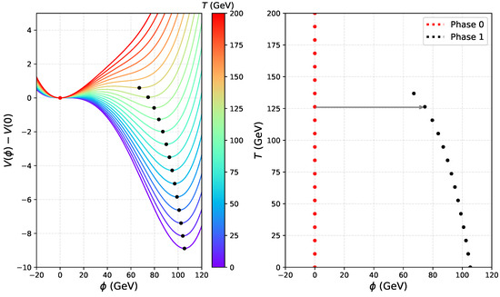
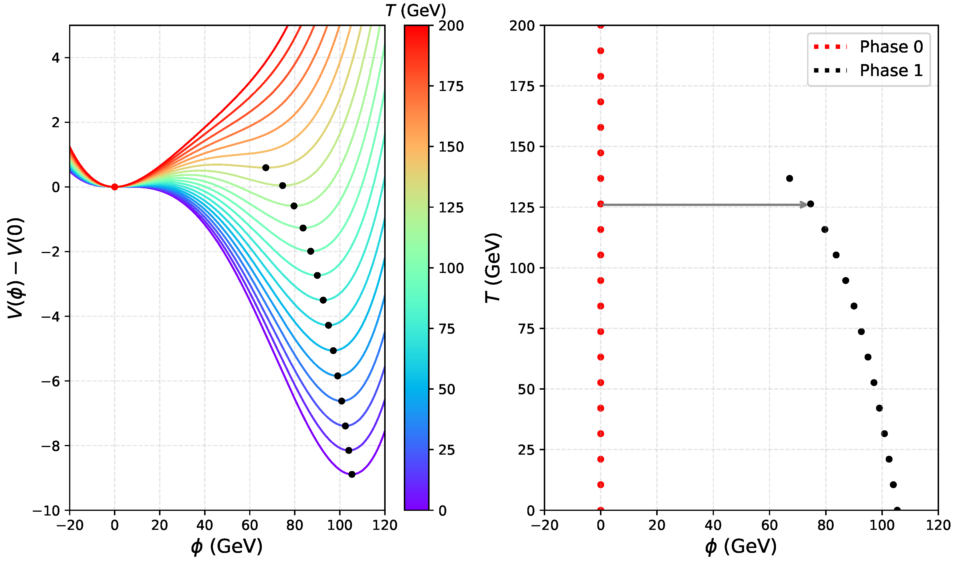
As shown in Figure 4, this method begins at a minimum corresponding to an extreme temperature—for instance, the non-zero minimum (black dot) in the zero-temperature effective potential (purple curve) in the left panel. Starting from this point, we increase the temperature by a step $\Delta T$ and estimate the new minimum using the field derivatives with respect to temperature, obtained by solving the Hessian matrix equation. The predicted position is then refined through a local optimization procedure (e.g., the Nelder–Mead method [104]) to locate the precise minimum. If the refined minimum lies sufficiently close to the predicted one, the two are regarded as belonging to the same phase. This minimum is saved, the temperature is increased again, and the process is repeated—this produces the sequence of black points in the right panel. If, instead, the refined minimum is not close to the predicted one, the step $\Delta T$ is reduced and a new prediction is made. The step size is decreased when the tracking encounters discontinuities or poor predictions, and increased when the evolution is smooth. Should $\Delta T$ be reduced to a prescribed tolerance while the refined minimum remains far from the predicted one, the current phase is considered to have ended. The predicted minimum then corresponds to the onset of a new phase, i.e., the red dot at $T\simeq 126\mathrm{GeV}$. From this point, the same tracking procedure is applied both forward and backward in temperature to trace the new phase.

Figure 4. Schematic of the tracing algorithm used to find phases and $T_C$. (Left): Effective potentials at different temperatures (colored curves). Local minimums are marked by black and red dots. (Right): minimums plotted in the $\varphi$–T plane, classified into two distinct phases. The critical temperature $T_C$ corresponds to the gray arrow.

To explore all possible phases, the above procedure is repeated for each minimum at extreme temperatures. CosmoTransitions employs user-provided approximations for the zero-temperature minimums as starting points, whereas PhaseTracer seeds its tracing algorithm with 50 random initial positions at both the zero-temperature and the user-specified maximum temperature. After all phases are identified, possible transitions between every two overlapping phases can be determined using the bisection method.

The main challenge in tracing a phase lies in identifying its endpoint, which typically corresponds to a saddle point where the potential is flat in one direction. This implies that the Hessian matrix has an eigenvalue of zero. However, confirming this numerically is difficult because we need a tolerance threshold to decide when a value is effectively zero. The problem is compounded when other eigenvalues are many orders of magnitude larger than the near-zero one, making it impractical to choose a single tolerance that works universally. Another common issue is that the potential may not be smooth due to numerical problems or model construction, leading to spurious local minimums and causing the calculation to fail.

At this stage, we can obtain the order parameter of electroweak FOPT from these tools,

$$\gamma ={\displaystyle \frac{v_C}{T_C}},$$

(8)

where $v_C$ is the non-zero expectation value of the Higgs at temperature $T_C$. Successful electroweak baryogenesis requires the EW sphaleron process to be out of equilibrium in the broken phase to ensure that the baryon asymmetry is not washed out. This condition can be translated into an approximate bound $\gamma \gtrsim 1$ [105]. BSMPT v2 can further calculate the baryon asymmetry of the Universe for the CP-violating 2HDM via two approximations, the semi-classical force approach [38] and the VEV-insertion approximation approach [39].

4. Transition Rates

In the presence of two minimums, the system may tunnel through the potential barrier via quantum effects or overcome it through thermal fluctuations, leading to the formation of bubbles in spacetime. The transition probability per unit time per unit volume at finite-temperature is given by [106,107]

$${\displaystyle \frac{\Gamma }{V}}=A\left(T\right)e^{-S\left(T\right)/T}[1+\mathcal{O}(\hslash )],$$

(9)

where $A\left(T\right)$ is a temperature-dependent prefactor and $S_E\left(T\right)$ is the Euclidean action,

$$S_E\left(T\right)=4\pi {\int }_0^{\infty }\mathrm{d}\rho {\rho }^2\left[{\displaystyle \frac{1}{2}}{\dot{\varphi }}^2+V\left(\varphi \right)\right].$$

(10)

Here $\rho =\sqrt{{\tau }^2+{\left|\overrightarrow{x}\right|}^2}$ and $\dot{\varphi }=\mathrm{d}\varphi /\mathrm{d}\rho$, $\tau$ represents the Euclidean (imaginary) time coordinate, $\overrightarrow{x}$ denotes the three-dimensional spatial coordinate vector in Euclidean space. The integration is performed over the bounce solution ${\varphi }_b$, an instanton that interpolates between the two phases. ${\varphi }_b$ satisfies the Euler–Lagrange equations

$$\ddot{\varphi }+{\displaystyle \frac{2}{\rho }}\dot{\varphi }=\nabla V\left(\varphi \right),$$

(11)

with boundary conditions

$${\left.\dot{\varphi }\right|}_{\rho =0}=0,{\left.\varphi \right|}_{\rho \to \infty }={\varphi }_f,$$

(12)

implying that the transition occurs at $\rho =0$, while far away the field remains in the false vacuum ${\varphi }_f$.

Accordingly, obtaining the bounce solution corresponds to solving a system of partial differential equations, which is a mathematical problem that remains an active research area. To address this challenge, a variety of numerical algorithms has been developed [108,109,110,111,112,113,114,115,116]. For one-dimensional potential, the over/under-shooting method proves both accurate and stable [117]. This approach frames the field evolution as a classical particle moving in an inverted potential $-V\left(\varphi \right)$, where $\varphi$ acts as a spatial coordinate and $\rho$ plays the role of time. It searches an initial field configuration ${\varphi }_0$ near the true vacuum ${\varphi }_t$, such that the field evolves to settle at the false vacuum ${\varphi }_f$ as $\rho \to \infty$. This method is widely used in phenomenological studies and is implemented in numerical tools such as CosmoTransitions, BSMPT v3, BubbleProfiler, and PhaseTracer2.

For multi-dimensional potentials, the path deformation method proposed in Refs. [54,118] is implemented in tools such as CosmoTransitions, BSMPT v3 and PhaseTracer2. This method decomposes the equations of motion into components parallel and perpendicular to an initial guess trajectory, then iteratively deforms the path toward the true bounce solution by applying corrections along the perpendicular direction. ELENA adopts the tunneling potential formalism [112], which converts the problem into an optimization task, offering improved speed and stability. However, it is currently limited to single-field potentials. Vevacious and TransitionListener relies on CosmoTransitions and PT2GWFinder uses FindBounce to obtain bounce profiles and actions.

Additionally, several dedicated tools have been developed. FindBounce implements the polygonal bounce method, a semi-analytic approach that discretizes the potential into piecewise-linear segments [119]. BubbleProfiler employs a perturbative technique for multifield potentials [108]. AnyBubble utilizes a multiple-shooting method, dividing the time domain into subintervals and stitching together local solutions to construct the global bounce. SimpleBounce treats the bounce solution as a fixed point of a gradient-flow equation.

Beyond these approaches, machine learning has also been applied to this problem. Ref. [114] employs neural networks to solve the differential equations relevant to bounce action computations. Ref. [120] trains a neural network to predict the bounce action directly from one-dimensional potentials, using 15 nodal values of the potential as input. Ref. [121] constructs a neural network that maps model parameters directly to the action curve.

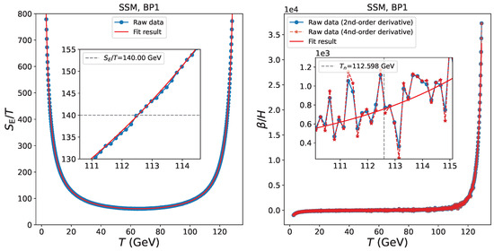
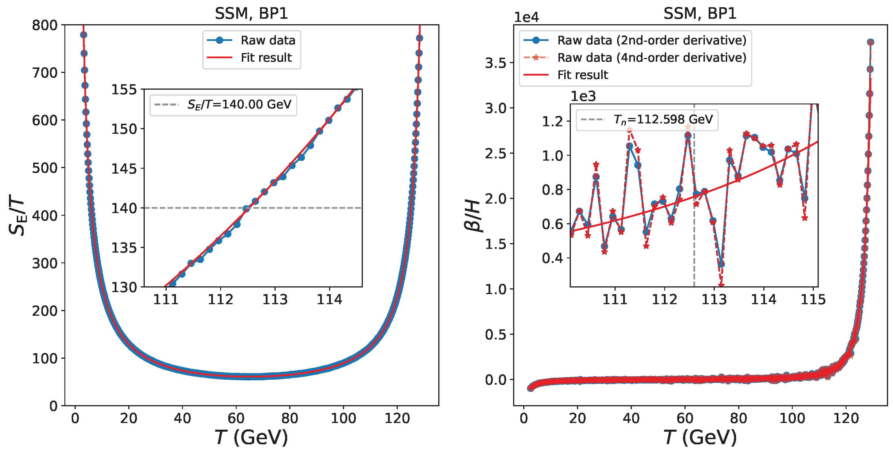
A prominent issue in the numerical computation of the action is instability and error. Ideally, the action should vary smoothly with temperature. However, as shown in Figure 5, we usually can observe a zigzag pattern. This irregular behavior will introduce non-negligible errors in the calculation of $\beta /H$, which will be introduced later. In addition to improving the computational accuracy of the action, fitting the temperature-dependent action function offers another viable approach. PhaseTracer2 applies a linear fit near the reference temperature to compute $\beta$. Vevacious approximates the straight-path Euclidean action $S^{\mathrm{straight}}$—representing the bounce action along a direct path from the false vacuum to the true vacuum—using ${(T_C-T)}^2$ multiplied by a polynomial in T, in order to estimate an upper bound for the survival probability. PT2GWFinder adopts a similar fitting strategy around the critical temperature $T_C$. Ref. [121] utilize the fitting function across the entire temperature range.

Figure 5. The variation of $S/T$ and $\beta /H$ with temperature for a example model, where the dotted lines represent the raw data and the solid lines represent the fitting results. This figure is taken from our previous work [121].

The prefactor $A\left(T\right)$ in Equation (9) arises from fluctuations around the saddle point. At leading order, these fluctuations contribute a quadratic term to the action and is given by [107,122]

$$A\left(T\right)=T{\left({\displaystyle \frac{S_E}{2\pi T}}\right)}^{\frac{3}{2}}{\left({\displaystyle \frac{{det}^{\prime }\left[-{\nabla }^2+V^{″}\left({\varphi }_b\right)\right]}{det\left[-{\nabla }^2+V^{″}\left({\varphi }_f\right)\right]}}\right)}^{-\frac{1}{2}},$$

(13)

where ${det}^{\prime }$ stands for the product of all eigenvalues excluding the zeros. BubbleDet automatically computes them and regularizes the sums for fluctuating scalar and gauge fields. The calculation related to the determinant term is challenging, so BSMPT v3, PT2GWFinder and ELENA adopts the approximation

$$A\left(T\right)\simeq T^4{\left({\displaystyle \frac{S}{2\pi T}}\right)}^{\frac{3}{2}},$$

(14)

while CosmoTransitions and PhaseTracer2 employ a further simplified version, $A\left(T\right)\simeq T^4$.

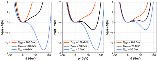
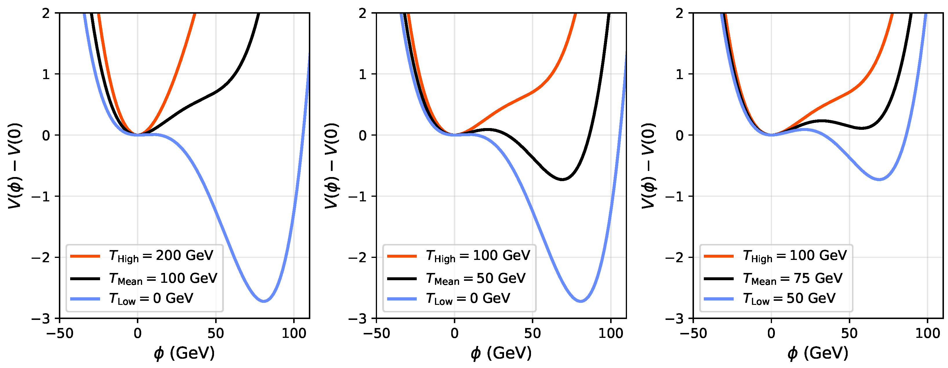
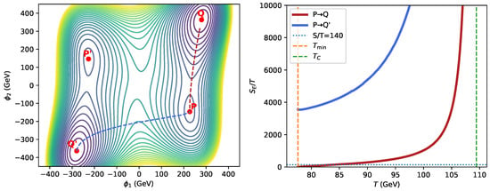
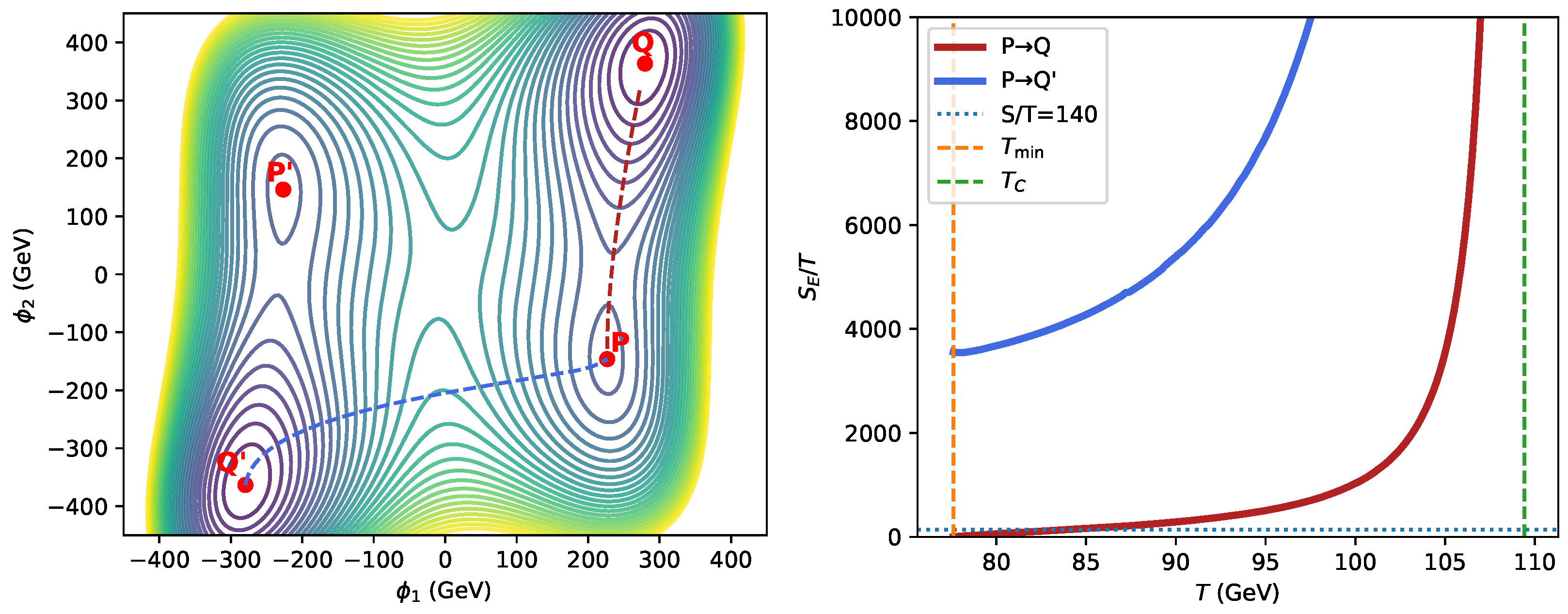
Finally, an important yet often overlooked issue is the discrete symmetry of the potential. As shown in Figure 6, consider two coexisting phases P and Q and their symmetry partners $P^{\prime }$ and $Q^{\prime }$ related by a $Z_2$ discrete symmetry. $P,P^{\prime }$ are false vacuums and $Q,Q^{\prime }$ are false vacuums. Four possible phase transitions can occur: $P\to Q$, $P^{\prime }\to Q$, $P\to Q^{\prime }$, and $P^{\prime }\to Q^{\prime }$. By discrete symmetry, the actions (tunneling barriers) satisfy

$$S(P\to Q)=S(P^{\prime }\to Q^{\prime }),S(P^{\prime }\to Q)=S(P\to Q^{\prime }),$$

(15)

but $S(P\to Q)$ may differ from $S(P\to Q^{\prime })$. These actions determine which transition the Universe follows. CosmoTransitions utilizes a user-defined function to carve out the symmetric field space. PhaseTracer selects the transition with the smallest action value to be the one that could have actually occurred in the model’s cosmological history. BSMPT v3 chooses the transitions with the shortest path between false and true vacuum.

Figure 6. Schematic illustration of $Z_2$ discrete symmetry in the potential. P and Q denote the false and true vacuums, with $P^{\prime }$ and $Q^{\prime }$ representing their symmetry partners. There are two unique transition path and the right panel shows the action curve corresponding to each path. This figure is taken from our previous work [59].

5. Transition Temperatures

In Equation (6), we define the critical temperature $T_C$ as the temperature at which the free energy densities of two phases become equal. It is relatively straightforward to compute, which is why $T_C$ is often treated as the phase transition temperature in simplified estimations. In reality, however, the actual phase transition does not occur at this temperature. The nucleation temperature $T_N$ is a more physically relevant quantity in practice.

The nucleation temperature is defined as the temperature at which, on average, one bubble nucleates per Hubble volume:

$$N\left(T_N\right)={\int }_{T_N}^{T_C}{\displaystyle \frac{\mathrm{d}T}{T}}{\displaystyle \frac{\Gamma \left(T\right)P_f\left(T\right)}{H{\left(T\right)}^4}}=1,$$

(16)

where $H\left(T\right)$ is Hubble parameter and $P_f\left(T\right)$ is the false vacuum fraction, given by [123,124]

$$P_f\left(T\right)=e^{-{\int }_{T_0}^T\mathrm{d}{T}^{\prime }\Gamma \left(T^{\prime }\right){\displaystyle \frac{a^3\left(T^{\prime }\right)}{a^3\left(T\right)}}\mathcal{V}(T^{\prime },T)}$$

(17)

where $\mathcal{V}(T^{\prime },T)$ denotes the fractional volume of a bubble at T that nucleated at temperature $T^{\prime }$. The fully accurate calculation is rather involved, but since the exponential term in Equation (9) dominates the behavior, the expression can be simplified to

$${\displaystyle \frac{\Gamma \left(T_N\right)}{H^4\left(T_N\right)}}=1.$$

(18)

For electroweak scale transition, it can be further simplified to

$$\begin{array}{}\mathrm{(19)}& \begin{array}{cc}{\displaystyle \frac{S_E}{T_N}}\hfill & \simeq 146-2ln\left({\displaystyle \frac{g_{\mathrm{eff}}^{\mathrm{tot}}}{100}}\right)-4ln\left({\displaystyle \frac{T_N}{100\mathrm{GeV}}}\right)\hfill \end{array}\mathrm{(20)}& \begin{array}{}& \begin{array}{cc}\hfill & \simeq 140.\hfill \end{array}\end{array}\hfill \end{array}$$

where $g_{\mathrm{eff}}^{\mathrm{tot}}$ is the total effective degree of freedom.

ELENA utilizes Equation (17) as it is for one scalar potential; BSMPT v3 adopts Equation (18); TransitionListener uses  Equation (19); CosmoTransitions and PhaseTracer2 utilize Equation (20); PT2GWFinder provides all the choices. Note that, as shown in Figure 5 and Figure 6, the $S/T$ may decrease monotonically as the temperature falls, but this is not always the case. The nucleation temperature is determined by selecting the first time where the condition in Equations (18)–(20) is satisfied.

For strongly supercooled transitions, the Universe remains in the false vacuum long after the vacuum becomes metastable, so cosmic expansion must be accounted for. In this case, the time of bubble collisions may occur much later than the nucleation time. Thus, using the percolation temperature is more reasonable when calculating GWs. The percolation temperature is defined as [125]

$$P_f\left(t_P\right)\approx 0.71.$$

(21)

Similarly, the completion temperature can be obtained by solving

$$P_f\left(t_F\right)=ϵ,$$

(22)

where $ϵ\ll 1$.

CosmoTransitions and TransitionListener provides the critical temperature $T_C$ and the nucleation temperature $T_N$. BSMPT v3, PhaseTracer2 combined with TransitionSolver, and ELENA are capable of delivering the full set of characteristic temperatures

6. Thermal Parameters

In addition to the transition temperatures, calculating phase transition GWs and baryon asymmetry requires other properties of the phase transition: the characteristic length scale, transition strength, bubble wall velocity, and so on. Here, we only cover the thermal parameters computed by the above tools, while calculations of more parameters, GWs, and baryon asymmetry are beyond the scope of this paper.

As the free energy density $\mathcal{F}=V$ and the pressure $p=-\mathcal{F}$, the energy density $\rho$, the enthalpy density $\omega$, and the entropy density s are given as

$$\begin{array}{c}\hfill \rho =V-T{\displaystyle \frac{\partial V}{\partial T}},w=-T{\displaystyle \frac{\partial V}{\partial T}},s=-{\displaystyle \frac{\partial V}{\partial T}}.\end{array}$$

(23)

The coefficient $\beta$ in the exponential nucleation rate $\Gamma \left(t\right)=\Gamma \left(t_{\ast }\right)e^{\beta (t-t\ast )}$ characterizes the inverse duration of the phase transition. Expanding the Euclidean action around $t_{\ast }$ to first order yields [126]

$$\beta ={\left.T_{\ast }{H}_{\ast }{\displaystyle \frac{d}{dT}}\left({\displaystyle \frac{S\left(T\right)}{T}}\right)\right|}_{T_{\ast }},$$

(24)

where $T_{\ast }$ is the reference temperature of the transition, and $t_{\ast }$ and $H_{\ast }$ denote the corresponding time and Hubble parameter at this temperature. PhaseTracer2, PT2GWFinder, TransitionListener and BSMPT v3 employ it in GWs calculations. Since its computation involves the differential of S, the numerical noise present in the calculation of S, as shown in Figure 6, has a strong impact on its evaluation. Thus, different fitting procedures are adopted in PhaseTracer2, Vevacious and PT2GWFinder to mitigate this issue. In addition, TransitionSolver and ELENA adopt the mean bubble separation R instead, which is derived from the bubble number density $n_B$ [123]

$$n_B=T^3{\int }_T^{T_c}d{T}^{\prime }{\displaystyle \frac{\Gamma \left(T^{\prime }\right)P_f\left(T^{\prime }\right)}{T^{\prime 4}H\left(T^{\prime }\right)}},R=n_B^{1/3}.$$

(25)

This approach offers advantages in treating strongly supercooled phase transitions.

The bubble wall velocity $v_w$ is another crucial parameter in gravitational wave predictions. It is time-dependent, as the bubble walls starting at rest and accelerating due to the pressure difference. The acceleration stage is typically short and can often be neglected. Determining the terminal wall velocity requires solving coupled scalar–fluid Boltzmann equations under non-equilibrium conditions, which remains a challenging task. Thus, it is commonly treated as an input parameter in tools such as PhaseTracer2, PT2GWFinder, TransitionSolver, ELENA and BSMPT v3. The latter two also offer approximate expressions based on Refs. [127,128]. There are also dedicated tools to compute $v_w$ more rigorously. WallGo implements the full treatment developed in Ref. [129]. Ref. [73] provides a code based on the local thermal equilibrium approximation.

The strength of FOPT is quantified by $\alpha$, the fraction of potential energy available for the the production of GWs. For the bag model, the vacuum energy is given by the bag constant $ϵ$, it is given as [130]

$$\alpha ={\displaystyle \frac{4ϵ}{3w_f\left(T_{\ast }\right)}},$$

(26)

where $w_f\left(T_{\ast }\right)$ is the enthalpy density far away from the bubble wall. In realistic models, it is usually defined by the trace anomaly as [131]

$$\alpha ={\displaystyle \frac{1}{{\pi }^2{g}_{\ast }{T}_{\ast }^4/30}}{\left[V\left({\varphi }_f\right)-V\left({\varphi }_t\right)-{\displaystyle \frac{T}{4}}\left({\displaystyle \frac{\partial V\left({\varphi }_f\right)}{\partial T}}-{\displaystyle \frac{\partial V\left({\varphi }_t\right)}{\partial T}}\right)\right]}_{T=T_{\ast }},$$

(27)

where $g_{\ast }$ represents the effective number of relativistic degrees of freedom at $T_{\ast }$. TransitionSolver implements both Equations (26) and (27); ELENA and TransitionListener adopts Equation (26); while PhaseTracer2, PT2GWFinder, and BSMPT v3 adopt Equation (27), despite slight differences in their respective treatments of $g_{\ast }$.

FOPT in the early Universe generates GWs through bubble wall collisions, sound waves and turbulence in the cosmic fluid. Each mechanism contributes a distinct power spectrum, and the total power spectrum is given by the sum of the three contributions. The resulting amplitudes and peak frequencies are governed by the phase transition temperature and the thermal parameters introduced above. PhaseTracer2, ELENA, TransitionListener, BSMPT v3, PT2GWFinder and TransitionSolver can output the GW power spectrum using fit formulae from analytic expresions [132,133,134,135,136,137]. There are also lattice simulation tools for simulating the nonlinear dynamics of the early universe to calculate GWs, such as CosmoLattice [138], HLattice [139], and PSpectRe [140], but these are beyond the scope of this review.

7. Conclusions

The studies of electroweak phase transition connect particle physics beyond the Standard Model to observable cosmological phenomena, including gravitational waves, baryogenesis, dark matter, and vacuum stability. They become particularly important as the direct searches for new physics at the LHC continue to return negative results. These studies drive advances in numerical tools to tackle the needed complex calculations. This review systematically outlines the key tools for analyzing cosmological phase transitions, as summarized in Table 1. It covers the construction of the finite-temperature effective potential, the tracing of phase histories, and the calculation of transition rates, milestone temperatures, and thermal parameters, together with an overview of the numerical tools for each step.

References

- Riotto, A.; Trodden, M. Recent progress in baryogenesis. Ann. Rev. Nucl. Part. Sci. 1999, 49, 35–75. [Google Scholar] [CrossRef] [Scilit]
- Mazumdar, A.; White, G. Review of cosmic phase transitions: Their significance and experimental signatures. Rep. Prog. Phys. 2019, 82, 076901. [Google Scholar] [CrossRef] [Scilit] [PubMed]
- Athron, P.; Balázs, C.; Fowlie, A.; Morris, L.; Wu, L. Cosmological phase transitions: From perturbative particle physics to gravitational waves. Prog. Part. Nucl. Phys. 2024, 135, 104094. [Google Scholar] [CrossRef] [Scilit]
- Cirelli, M.; Strumia, A.; Zupan, J. Dark Matter. arXiv 2024, arXiv:2406.01705. [Google Scholar] [CrossRef] [Scilit]
- Navas, S.; Amsler, C.; Gutsche, T.; Hanhart, C.; Hernández-Rey, J.J.; Lourenço, C.; Masoni, A.; Mikhasenko, M.; Mitchell, R.E.; Patrignani, C.; et al. Review of particle physics. Phys. Rev. D 2024, 110, 030001. [Google Scholar] [CrossRef] [Scilit]
- Sopczak, A. Higgs Boson Searches at the LHC Beyond the Standard Model. Physics 2024, 6, 1132–1170. [Google Scholar] [CrossRef] [Scilit]
- Wang, L.; Yang, J.M.; Zhang, Y.; Zhu, P.; Zhu, R. A Concise Review on Some Higgs-Related New Physics Models in Light of Current Experiments. Universe 2023, 9, 178. [Google Scholar] [CrossRef] [Scilit]
- Wang, F.; Wang, W.; Yang, J.; Zhang, Y.; Zhu, B. Low Energy Supersymmetry Confronted with Current Experiments: An Overview. Universe 2022, 8, 178. [Google Scholar] [CrossRef] [Scilit]
- Trocino, D. Searches in the long-lived particle and dark sectors. In Proceedings of the 35th Rencontres de Blois: Particle Physics and Cosmology, Blois, France, 20–25 October 2024. [Google Scholar]
- Neutelings, I. Leptoquark searches at ATLAS and CMS. In Proceedings of the 58th Rencontres de Moriond on Electroweak Interactions and Unified Theories, La Thuile, Italy, 24–31 March 2024. [Google Scholar]
- Seidita, R. Dark sector searches at ATLAS and CMS. PoS 2025, 489, 032. [Google Scholar] [CrossRef] [Scilit]
- Hirose, S. Search for rare Higgs boson decays and BSM Higgs bosons. PoS 2026, 478, 186. [Google Scholar] [CrossRef] [Scilit]
- Abbott, B.P. et al. [LIGO Scientific Collaboration and Virgo Collaboration] GWTC-1: A Gravitational-Wave Transient Catalog of Compact Binary Mergers Observed by LIGO and Virgo during the First and Second Observing Runs. Phys. Rev. X 2019, 9, 031040. [Google Scholar] [CrossRef] [Scilit]
- Abbott, B.P. et al. [LIGO Scientific Collaboration and Virgo Collaboration] Binary Black Hole Population Properties Inferred from the First and Second Observing Runs of Advanced LIGO and Advanced Virgo. Astrophys. J. Lett. 2019, 882, L24. [Google Scholar] [CrossRef] [Scilit]
- Aasi, J. et al. [LIGO Scientific Collaboration] Advanced LIGO. Class. Quant. Grav. 2015, 32, 074001. [Google Scholar] [CrossRef] [Scilit]
- Acernese, F.; Agathos, M.; Agatsuma, K.; Aisa, D.; Allemandou, N.; Allocca, A.; Amarni, J.; Astone, P.; Balestri, G.; Ballardin, G.; et al. Advanced Virgo: A second-generation interferometric gravitational wave detector. Class. Quant. Grav. 2015, 32, 024001. [Google Scholar] [CrossRef] [Scilit]
- Akutsu, T.; Ando, M.; Arai, K.; Arai, Y.; Araki, S.; Araya, A.; Aritomi, N.; Aso, Y.; Bae, S.; Bae, Y.; et al. Overview of KAGRA: Detector design and construction history. Prog. Theor. Exp. Phys. 2021, 2021, 05A101. [Google Scholar] [CrossRef] [Scilit]
- Xu, H.; Chen, S.; Guo, Y.; Jiang, J.; Wang, B.; Xu, J.; Xue, Z.; Caballero, R.N.; Yuan, J.; Xu, Y.; et al. Searching for the nano-hertz stochastic gravitational wave background with the Chinese pulsar timing array data release I. Res. Astron. Astrophys. 2023, 23, 075024. [Google Scholar] [CrossRef] [Scilit]
- Reardon, D.J.; Zic, A.; Shannon, R.M.; Hobbs, G.B.; Bailes, M.; Di Marco, V.; Kapur, A.; Rogers, A.F.; Thrane, E.; Askew, J.; et al. Search for an isotropic gravitational-wave background with the parkes pulsar timing array. Astrophys. J. Lett. 2023, 951, 1. [Google Scholar] [CrossRef] [Scilit]
- Antoniadis, J. et al. [EPTA Collaboration and InPTA Collaboration] The second data release from the European Pulsar Timing Array—III. Search for gravitational wave signals. Astron. Astrophys. 2023, 678, A50. [Google Scholar] [CrossRef] [Scilit]
- Agazie, G.; Anumarlapudi, A.; Archibald, A.M.; Arzoumanian, Z.; Baker, P.T.; Bécsy, B.; Blecha, L.; Brazier, A.; Brook, P.R.; Burke-Spolaor, S.; et al. The NANOGrav 15 yr Data Set: Evidence for a Gravitational-wave Background. Astrophys. J. Lett. 2023, 951, L8. [Google Scholar] [CrossRef] [Scilit]
- Amaro-Seoane, P.; Audley, H.; Babak, S.; Baker, J.; Barausse, E.; Bender, P.; Berti, E.; Binetruy, P.; Born, M.; Bortoluzzi, D.; et al. Laser Interferometer Space Antenna. arXiv 2017, arXiv:1702.00786. [Google Scholar] [CrossRef] [Scilit]
- Hu, W.R.; Wu, Y.L. The Taiji Program in Space for gravitational wave physics and the nature of gravity. Natl. Sci. Rev. 2017, 4, 685–686. [Google Scholar] [CrossRef] [Scilit]
- Luo, J.; Chen, L.-S.; Duan, H.-Z.; Gong, Y.-G.; Hu, S.; Ji, J.; Liu, Q.; Mei, J.; Milyukov, V.; Sazhin, M.; et al. TianQin: A space-borne gravitational wave detector. Class. Quant. Grav. 2016, 33, 035010. [Google Scholar] [CrossRef] [Scilit]
- Schnabel, R.; Korobko, M. Optical sensitivities of current gravitational wave observatories at higher kHz, MHz and GHz frequencies. Sci. Rep. 2025, 15, 25733. [Google Scholar] [CrossRef] [Scilit] [PubMed]
- Carney, D.; Higgins, G.; Marocco, G.; Wentzel, M. Superconducting Levitated Detector of Gravitational Waves. Phys. Rev. Lett. 2025, 134, 181402. [Google Scholar] [CrossRef] [Scilit]
- Cai, R.G.; Cao, Z.; Guo, Z.K.; Wang, S.J.; Yang, T. The Gravitational-Wave Physics. Natl. Sci. Rev. 2017, 4, 687–706. [Google Scholar] [CrossRef] [Scilit]
- Caprini, C.; Chala, M.; Dorsch, G.C.; Hindmarsh, M.; Huber, S.J.; Konstandin, T.; Kozaczuk, J.; Nardini, G.; No, J.M.; Rummukainen, K.; et al. Detecting gravitational waves from cosmological phase transitions with LISA: An update. J. Cosmol. Astropart. Phys. 2020, 3, 24. [Google Scholar] [CrossRef] [Scilit]
- Hindmarsh, M.B.; Lüben, M.; Lumma, J.; Pauly, M. Phase transitions in the early universe. SciPost Phys. Lect. Notes 2021, 24, 1. [Google Scholar] [CrossRef] [Scilit]
- Bian, L.; Cai, R.-G.; Cao, S.; Cao, Z.; Gao, H.; Guo, Z.-K.; Lee, K.; Li, D.; Liu, J.; Lu, Y.; et al. The Gravitational-wave physics II: Progress. Sci. China Phys. Mech. Astron. 2021, 64, 120401. [Google Scholar] [CrossRef] [Scilit]
- D’Onofrio, M.; Rummukainen, K.; Tranberg, A. Sphaleron Rate in the Minimal Standard Model. Phys. Rev. Lett. 2014, 113, 141602. [Google Scholar] [CrossRef] [Scilit]
- Athron, P.; Balazs, C.; Fowlie, A.; Pozzo, G.; White, G.; Zhang, Y. Strong first-order phase transitions in the NMSSM—A comprehensive survey. J. High Energy Phys. 2019, 11, 151. [Google Scholar] [CrossRef] [Scilit]
- Han, X.F.; Wang, L.; Zhang, Y. Dark matter, electroweak phase transition, and gravitational waves in the type II two-Higgs-doublet model with a singlet scalar field. Phys. Rev. D 2021, 103, 035012. [Google Scholar] [CrossRef] [Scilit]
- Xiao, Y.; Yang, J.M.; Zhang, Y. Implications of nano-Hertz gravitational waves on electroweak phase transition in the singlet dark matter model. Sci. Bull. 2023, 68, 3158–3164. [Google Scholar] [CrossRef] [Scilit] [PubMed]
- Si, Z.-g.; Wang, H.-x.; Wang, L.; Zhang, Y. Exploring multi-step electroweak phase transitions in the 2HDM+a. Eur. Phys. J. C 2025, 85, 273. [Google Scholar] [CrossRef] [Scilit]
- Li, S.; Yang, J.M.; Zhang, M.; Zhang, Y.; Zhu, R. Can a secluded self-interacting dark sector generate detectable gravitational waves? arXiv 2025, arXiv:2502.04108. [Google Scholar] [CrossRef] [Scilit]
- Guan, S.; Guo, H.K.; Jiao, D.; Liang, Q.; Wu, L.; Zhang, Y. Measuring Gravitational Wave Spectrum from Electroweak Phase Transition and Higgs Self-Couplings. arXiv 2025, arXiv:2511.00996. [Google Scholar] [CrossRef] [Scilit]
- Trodden, M. Electroweak baryogenesis. Rev. Mod. Phys. 1999, 71, 1463–1500. [Google Scholar] [CrossRef] [Scilit]
- Morrissey, D.E.; Ramsey-Musolf, M.J. Electroweak baryogenesis. New J. Phys. 2012, 14, 125003. [Google Scholar] [CrossRef] [Scilit]
- Biekötter, T.; Heinemeyer, S.; Weiglein, G. Vacuum (meta-)stability in the μνSSM. Eur. Phys. J. C 2022, 82, 301. [Google Scholar] [CrossRef] [Scilit]
- Biekötter, T.; Heinemeyer, S.; No, J.M.; Olea-Romacho, M.O.; Weiglein, G. The trap in the early Universe: Impact on the interplay between gravitational waves and LHC physics in the 2HDM. J. Cosmol. Astropart. Phys. 2023, 3, 31. [Google Scholar] [CrossRef] [Scilit]
- Arsenault, A.; Cingiloglu, K.Y.; Frank, M. Vacuum stability in the Standard Model with vectorlike fermions. Phys. Rev. D 2023, 107, 036018. [Google Scholar] [CrossRef] [Scilit]
- Balázs, C.; Xiao, Y.; Yang, J.M.; Zhang, Y. New vacuum stability limit from cosmological history. Nucl. Phys. B 2024, 1002, 116533. [Google Scholar] [CrossRef] [Scilit]
- Wainwright, C.; Profumo, S. The Impact of a strongly first-order phase transition on the abundance of thermal relics. Phys. Rev. D 2009, 80, 103517. [Google Scholar] [CrossRef] [Scilit]
- Baker, M.J.; Kopp, J.; Long, A.J. Filtered Dark Matter at a First Order Phase Transition. Phys. Rev. Lett. 2020, 125, 151102. [Google Scholar] [CrossRef] [Scilit] [PubMed]
- Baker, M.J.; Kopp, J. Dark Matter Decay between Phase Transitions at the Weak Scale. Phys. Rev. Lett. 2017, 119, 061801. [Google Scholar] [CrossRef] [Scilit] [PubMed]
- Baker, M.J.; Mittnacht, L. Variations on the Vev Flip-Flop: Instantaneous Freeze-out and Decaying Dark Matter. J. High Energy Phys. 2019, 5, 70. [Google Scholar] [CrossRef] [Scilit]
- Bian, L.; Liu, X. Two-step strongly first-order electroweak phase transition modified FIMP dark matter, gravitational wave signals, and the neutrino mass. Phys. Rev. D 2019, 99, 055003. [Google Scholar] [CrossRef] [Scilit]
- Wong, X.R.; Xie, K.P. Freeze-in of WIMP dark matter. Phys. Rev. D 2023, 108, 055035. [Google Scholar] [CrossRef] [Scilit]
- Chung, D.; Long, A.; Wang, L.T. Probing the Cosmological Constant and Phase Transitions with Dark Matter. Phys. Rev. D 2011, 84, 043523. [Google Scholar] [CrossRef] [Scilit]
- Xiao, Y.; Yang, J.M.; Zhang, Y. Dilution of dark matter relic density in singlet extension models. J. High Energy Phys. 2023, 2, 8. [Google Scholar] [CrossRef] [Scilit]
- Roy, S. Dilution of dark matter relic abundance due to first order electroweak phase transition in the singlet scalar extended type-II seesaw model. Phys. Rev. D 2025, 111, 015037. [Google Scholar] [CrossRef] [Scilit]
- Wang, W.; Xu, W.L.; Yang, J.M. A hidden self-interacting dark matter sector with first-order cosmological phase transition and gravitational wave. Eur. Phys. J. Plus 2023, 138, 781. [Google Scholar] [CrossRef] [Scilit]
- Wainwright, C.L. CosmoTransitions: Computing Cosmological Phase Transition Temperatures and Bubble Profiles with Multiple Fields. Comput. Phys. Commun. 2012, 183, 2006–2013. [Google Scholar] [CrossRef] [Scilit]
- Basler, P.; Mühlleitner, M. BSMPT (Beyond the Standard Model Phase Transitions): A tool for the electroweak phase transition in extended Higgs sectors. Comput. Phys. Commun. 2019, 237, 62–85. [Google Scholar] [CrossRef] [Scilit]
- Basler, P.; Mühlleitner, M.; Müller, J. BSMPT v2 a tool for the electroweak phase transition and the baryon asymmetry of the universe in extended Higgs Sectors. Comput. Phys. Commun. 2021, 269, 108124. [Google Scholar] [CrossRef] [Scilit]
- Basler, P.; Biermann, L.; Mühlleitner, M.; Müller, J.; Santos, R.; Viana, J. BSMPT v3 a tool for phase transitions and primordial gravitational waves in extended Higgs sectors. Comput. Phys. Commun. 2025, 316, 109766. [Google Scholar] [CrossRef] [Scilit]
- Athron, P.; Balázs, C.; Fowlie, A.; Zhang, Y. PhaseTracer: Tracing cosmological phases and calculating transition properties. Eur. Phys. J. C 2020, 80, 567. [Google Scholar] [CrossRef] [Scilit]
- Athron, P.; Balazs, C.; Fowlie, A.; Morris, L.; Searle, W.; Xiao, Y.; Zhang, Y. PhaseTracer2: From the effective potential to gravitational waves. Eur. Phys. J. C 2025, 85, 559. [Google Scholar] [CrossRef] [Scilit]
- Ertas, F.; Kahlhoefer, F.; Tasillo, C. Turn up the volume: Listening to phase transitions in hot dark sectors. J. Cosmol. Astropart. Phys. 2022, 2, 14. [Google Scholar] [CrossRef] [Scilit]
- Brdar, V.; Finetti, M.; Matteini, M.; Morais, A.P.; Nemevšek, M. PT2GWFinder: A Package for Cosmological First-Order Phase Transitions and Gravitational Waves. arXiv 2025, arXiv:2505.04744. [Google Scholar] [CrossRef] [Scilit]
- Costa, F.; Hoefken Zink, J.; Lucente, M.; Pascoli, S.; Rosauro-Alcaraz, S. ELENA: A software for fast and precise computation of first order phase transitions and gravitational waves production in particle physics models. arXiv 2025, arXiv:2510.00289. [Google Scholar] [CrossRef] [Scilit]
- Masoumi, A.; Olum, K.D.; Shlaer, B. Efficient numerical solution to vacuum decay with many fields. J. Cosmol. Astropart. Phys. 2017, 1, 51. [Google Scholar] [CrossRef] [Scilit]
- Athron, P.; Balázs, C.; Bardsley, M.; Fowlie, A.; Harries, D.; White, G. BubbleProfiler: Finding the field profile and action for cosmological phase transitions. Comput. Phys. Commun. 2019, 244, 448–468. [Google Scholar] [CrossRef] [Scilit]
- Sato, R. SimpleBounce: A simple package for the false vacuum decay. Comput. Phys. Commun. 2021, 258, 107566, Erratum in Comput. Phys. Commun. 2026, 320, 110006. [Google Scholar] [CrossRef] [Scilit]
- Guada, V.; Nemevšek, M.; Pintar, M. FindBounce: Package for multi-field bounce actions. Comput. Phys. Commun. 2020, 256, 107480. [Google Scholar] [CrossRef] [Scilit]
- Camargo-Molina, J.E.; O’Leary, B.; Porod, W.; Staub, F. Vevacious: A Tool For Finding The Global Minima of One-Loop Effective Potentials With Many Scalars. Eur. Phys. J. C 2013, 73, 2588. [Google Scholar] [CrossRef] [Scilit]
- Fowlie, A. A fast C++ implementation of thermal functions. Comput. Phys. Commun. 2018, 228, 264–272. [Google Scholar] [CrossRef] [Scilit]
- Ekstedt, A.; Schicho, P.; Tenkanen, T.V.I. DRalgo: A package for effective field theory approach for thermal phase transitions. Comput. Phys. Commun. 2023, 288, 108725. [Google Scholar] [CrossRef] [Scilit]
- Ekstedt, A.; Gould, O.; Hirvonen, J.; Laurent, B.; Niemi, L.; Schicho, P.; van de Vis, J. How fast does the WallGo? A package for computing wall velocities in first-order phase transitions. J. High Energy Phys. 2025, 4, 101. [Google Scholar] [CrossRef] [Scilit]
- van de Vis, J.; Schicho, P.; Niemi, L.; Laurent, B.; Hirvonen, J.; Gould, O. WallGo investigates: Theoretical uncertainties in the bubble wall velocity. arXiv 2025, arXiv:2510.27691. [Google Scholar] [CrossRef] [Scilit]
- Ekstedt, A.; Gould, O.; Hirvonen, J. BubbleDet: A Python package to compute functional determinants for bubble nucleation. J. High Energy Phys. 2023, 12, 56. [Google Scholar] [CrossRef] [Scilit]
- Si, Z.; Wang, H.; Wang, L.; Xiao, Y.; Zhang, Y. The bubble wall velocity in local thermal equilibrium and energy budget with full effective potential. J. High Energy Phys. 2025, 2025, 29. [Google Scholar] [CrossRef] [Scilit]
- Patel, H.H.; Ramsey-Musolf, M.J. Baryon Washout, Electroweak Phase Transition, and Perturbation Theory. J. High Energy Phys. 2011, 7, 29. [Google Scholar] [CrossRef] [Scilit]
- Athron, P.; Balazs, C.; Fowlie, A.; Morris, L.; White, G.; Zhang, Y. How arbitrary are perturbative calculations of the electroweak phase transition? J. High Energy Phys. 2023, 2023, 50. [Google Scholar] [CrossRef] [Scilit]
- Sher, M. Electroweak Higgs potential and vacuum stability. Phys. Rep. 1989, 179, 273–418. [Google Scholar] [CrossRef] [Scilit]
- Quiros, M. Finite temperature field theory and phase transitions. In Proceedings of the ICTP Summer School in High-Energy Physics and Cosmology; World Scientific: Singapore, 1999; pp. 187–259. [Google Scholar]
- Zinn-Justin, J. Quantum field theory at finite temperature: An Introduction. arXiv 2000, arXiv:hep-ph/0005272. [Google Scholar] [CrossRef] [Scilit]
- Laine, M.; Vuorinen, A. Basics of Thermal Field Theory; Springer: Berlin/Heidelberg, Germany, 2016; Volume 925. [Google Scholar] [CrossRef] [Scilit]
- Parwani, R.R. Resummation in a hot scalar field theory. Phys. Rev. D 1992, 45, 4695, Erratum in Phys. Rev. D 1993, 48, 5965. [Google Scholar] [CrossRef] [Scilit]
- Arnold, P.B.; Espinosa, O. The Effective potential and first order phase transitions: Beyond leading-order. Phys. Rev. D 1993, 47, 3546, Erratum in Phys. Rev. D 1994, 50, 6662. [Google Scholar] [CrossRef] [Scilit]
- Appelquist, T.; Pisarski, R.D. High-temperature Yang-Mills theories and three-dimensional quantum chromodynamics. Phys. Rev. D 1981, 23, 2305–2317. [Google Scholar] [CrossRef] [Scilit]
- Ginsparg, P. First and second order phase transitions in gauge theories at finite temperature. Nucl. Phys. B 1980, 170, 388–408. [Google Scholar] [CrossRef] [Scilit]
- Laine, M.; Meyer, M.; Nardini, G. Thermal phase transition with full 2-loop effective potential. Nucl. Phys. B 2017, 920, 565–600. [Google Scholar] [CrossRef] [Scilit]
- Ekstedt, A.; Löfgren, J. A Critical Look at the Electroweak Phase Transition. J. High Energy Phys. 2020, 12, 136. [Google Scholar] [CrossRef] [Scilit]
- Kainulainen, K.; Keus, V.; Niemi, L.; Rummukainen, K.; Tenkanen, T.V.I.; Vaskonen, V. On the validity of perturbative studies of the electroweak phase transition in the Two Higgs Doublet model. J. High Energy Phys. 2019, 2019, 75. [Google Scholar] [CrossRef] [Scilit]
- Wolfram Research, I. Mathematica 14.0. 2024. Available online: https://www.wolfram.com/mathematica/ (accessed on 20 February 2026).
- Staub, F. Exploring new models in all detail with SARAH. Adv. High Energy Phys. 2015, 2015, 840780. [Google Scholar] [CrossRef] [Scilit]
- Virtanen, P.; Gommers, R.; Oliphant, T.E.; Haberland, M.; Reddy, T.; Cournapeau, D.; Burovski, E.; Peterson, P.; Weckesser, W.; Bright, J.; et al. SciPy 1.0: Fundamental Algorithms for Scientific Computing in Python; Nature Research: London, UK, 2020. [Google Scholar] [CrossRef] [Scilit]
- Fowlie, A. thermal_funcs: Thermal Functions for Finite-Temperature Effective Field-Theory in C++ with Python and Mathematica Interfaces. GitHub Repository. 2024. Available online: https://github.com/andrewfowlie/thermal_funcs (accessed on 20 February 2026).
- Piessens, R.; de Doncker-Kapenga, E.; Überhuber, C.; Kahaner, D. QUADPACK: A Subroutine Package for Automatic Integration; Springer Series in Computational Mathematics; Springer: Berlin/Heidelberg, Germany, 1983; Volume 1. [Google Scholar] [CrossRef] [Scilit]
- Coimbra, R.; Sampaio, M.O.P.; Santos, R. ScannerS: Constraining the phase diagram of a complex scalar singlet at the LHC. Eur. Phys. J. C 2013, 73, 2428. [Google Scholar] [CrossRef] [Scilit]
- Biekötter, T.; Olea-Romacho, M.O. Benchmarking a fading window: Electroweak baryogenesis in the C2HDM, LHC constraints after Run 2 and prospects for LISA. J. High Energy Phys. 2025, 2025, 40. [Google Scholar] [CrossRef] [Scilit]
- Biekötter, T.; Grohsjean, A.; Heinemeyer, S.; Schwanenberger, C.; Weiglein, G. Possible indications for new Higgs bosons in the reach of the LHC: N2HDM and NMSSM interpretations. Eur. Phys. J. C 2022, 82, 178. [Google Scholar] [CrossRef] [Scilit]
- Del Cima, O.M.; Franco, D.H.T.; Piguet, O. Gauge independence of the effective potential revisited. Nucl. Phys. B 1999, 551, 813–825. [Google Scholar] [CrossRef] [Scilit]
- Nielsen, N. On the gauge dependence of spontaneous symmetry breaking in gauge theories. Nucl. Phys. B 1975, 101, 173–188. [Google Scholar] [CrossRef] [Scilit]
- Del Cima, O.M. Probing the Nielsen identities. Phys. Lett. B 1999, 457, 307–310. [Google Scholar] [CrossRef] [Scilit]
- Nielsen, N.K. Removing the gauge parameter dependence of the effective potential by a field redefinition. Phys. Rev. D 2014, 90, 036008. [Google Scholar] [CrossRef] [Scilit]
- Di Luzio, L.; Mihaila, L. On the gauge dependence of the Standard Model vacuum instability scale. J. High Energy Phys. 2014, 2014, 79. [Google Scholar] [CrossRef] [Scilit]
- Espinosa, J.R.; Garny, M.; Konstandin, T. Interplay of Infrared Divergences and Gauge-Dependence of the Effective Potential. Phys. Rev. D 2016, 94, 055026. [Google Scholar] [CrossRef] [Scilit]
- Athron, P.; Bach, M.; Harries, D.; Kwasnitza, T.; Park, J.h.; Stöckinger, D.; Voigt, A.; Ziebell, J. FlexibleSUSY 2.0: Extensions to investigate the phenomenology of SUSY and non-SUSY models. Comput. Phys. Commun. 2018, 230, 145–217. [Google Scholar] [CrossRef] [Scilit]
- Searle, W.; Balázs, C.; Xiao, Y.; Zhang, Y. Machine learning left-right breaking from gravitational waves. J. Cosmol. Astropart. Phys. 2025, 11, 34. [Google Scholar] [CrossRef] [Scilit]
- Vaskonen, V. Electroweak baryogenesis and gravitational waves from a real scalar singlet. Phys. Rev. D 2017, 95, 123515. [Google Scholar] [CrossRef] [Scilit]
- Nelder, J.A.; Mead, R. A Simplex Method for Function Minimization. Comput. J. 1965, 7, 308–313. [Google Scholar] [CrossRef] [Scilit]
- Moore, G.D. Measuring the broken phase sphaleron rate nonperturbatively. Phys. Rev. D 1999, 59, 014503. [Google Scholar] [CrossRef] [Scilit]
- Linde, A.D. Fate of the false vacuum at finite temperature: Theory and applications. Phys. Lett. B 1981, 100, 37–40. [Google Scholar] [CrossRef] [Scilit]
- Linde, A. Decay of the false vacuum at finite temperature. Nucl. Phys. B 1983, 223, 544. [Google Scholar] [CrossRef] [Scilit]
- Akula, S.; Balázs, C.; White, G.A. Semi-analytic techniques for calculating bubble wall profiles. Eur. Phys. J. C 2016, 76, 681. [Google Scholar] [CrossRef] [Scilit]
- Andreassen, A.; Farhi, D.; Frost, W.; Schwartz, M.D. Direct Approach to Quantum Tunneling. Phys. Rev. Lett. 2016, 117, 231601. [Google Scholar] [CrossRef] [Scilit]
- Brown, A.R. Thin-wall approximation in vacuum decay: A lemma. Phys. Rev. D 2018, 97, 105002. [Google Scholar] [CrossRef] [Scilit]
- Espinosa, J.R.; Konstandin, T. A Fresh Look at the Calculation of Tunneling Actions in Multi-Field Potentials. J. Cosmol. Astropart. Phys. 2019, 1, 51. [Google Scholar] [CrossRef] [Scilit]
- Espinosa, J.R. A Fresh Look at the Calculation of Tunneling Actions. J. Cosmol. Astropart. Phys. 2018, 7, 36. [Google Scholar] [CrossRef] [Scilit]
- Braden, J.; Johnson, M.C.; Peiris, H.V.; Pontzen, A.; Weinfurtner, S. New Semiclassical Picture of Vacuum Decay. Phys. Rev. Lett. 2019, 123, 031601, Erratum in Phys. Rev. Lett. 2022, 129, 059901. [Google Scholar] [CrossRef] [Scilit] [PubMed]
- Piscopo, M.L.; Spannowsky, M.; Waite, P. Solving differential equations with neural networks: Applications to the calculation of cosmological phase transitions. Phys. Rev. D 2019, 100, 016002. [Google Scholar] [CrossRef] [Scilit]
- Sato, R. Simple Gradient Flow Equation for the Bounce Solution. Phys. Rev. D 2020, 101, 016012. [Google Scholar] [CrossRef] [Scilit]
- Bardsley, M. An optimisation based algorithm for finding the nucleation temperature of cosmological phase transitions. Comput. Phys. Commun. 2022, 273, 108252. [Google Scholar] [CrossRef] [Scilit]
- Coleman, S. Erratum: Fate of the false vacuum: Semiclassical theory. Phys. Rev. D 1977, 16, 1248. [Google Scholar] [CrossRef] [Scilit]
- Cline, J.M.; Moore, G.D.; Servant, G. Was the electroweak phase transition preceded by a color broken phase? Phys. Rev. D 1999, 60, 105035. [Google Scholar] [CrossRef] [Scilit]
- Guada, V.; Maiezza, A.; Nemevšek, M. Multifield Polygonal Bounces. Phys. Rev. D 2019, 99, 056020. [Google Scholar] [CrossRef] [Scilit]
- Jinno, R. Machine learning for bounce calculation. arXiv 2018, arXiv:1805.12153. [Google Scholar] [CrossRef] [Scilit]
- Bian, L.; Wang, H.; Xiao, Y.; Yang, J.C.; Yang, J.M.; Zhang, Y. Enhancing Phase Transition Calculations with Fitting and Neural Network. arXiv 2025, arXiv:2510.10667. [Google Scholar] [CrossRef] [Scilit]
- Callan, C.G.; Coleman, S. Fate of the false vacuum. II. First quantum corrections. Phys. Rev. D 1977, 16, 1762–1768. [Google Scholar] [CrossRef] [Scilit]
- Guth, A.H.; Tye, S.H.H. Phase Transitions and Magnetic Monopole Production in the Very Early Universe. Phys. Rev. Lett. 1980, 44, 631–635. [Google Scholar] [CrossRef] [Scilit]
- Guth, A.H.; Weinberg, E.J. Cosmological consequences of a first-order phase transition in the SU5 grand unified model. Phys. Rev. D 1981, 23, 876–885. [Google Scholar] [CrossRef] [Scilit]
- Athron, P.; Balázs, C.; Morris, L. Supercool subtleties of cosmological phase transitions. J. Cosmol. Astropart. Phys. 2023, 3, 6. [Google Scholar] [CrossRef] [Scilit]
- Ellis, J.; Lewicki, M.; No, J.M. On the Maximal Strength of a First-Order Electroweak Phase Transition and its Gravitational Wave Signal. J. Cosmol. Astropart. Phys. 2019, 4, 3. [Google Scholar] [CrossRef] [Scilit]
- Lewicki, M.; Merchand, M.; Zych, M. Electroweak bubble wall expansion: Gravitational waves and baryogenesis in Standard Model-like thermal plasma. J. High Energy Phys. 2022, 2022, 17. [Google Scholar] [CrossRef] [Scilit]
- Ellis, J.; Lewicki, M.; Merchand, M.; No, J.M.; Zych, M. The scalar singlet extension of the Standard Model: Gravitational waves versus baryogenesis. J. High Energy Phys. 2023, 2023, 93. [Google Scholar] [CrossRef] [Scilit]
- Laurent, B.; Cline, J.M. First principles determination of bubble wall velocity. Phys. Rev. D 2022, 106, 023501. [Google Scholar] [CrossRef] [Scilit]
- Espinosa, J.R.; Konstandin, T.; No, J.M.; Servant, G. Energy Budget of Cosmological First-order Phase Transitions. J. Cosmol. Astropart. Phys. 2010, 6, 28. [Google Scholar] [CrossRef] [Scilit]
- Hindmarsh, M.; Huber, S.J.; Rummukainen, K.; Weir, D.J. Numerical simulations of acoustically generated gravitational waves at a first order phase transition. Phys. Rev. D 2015, 92, 123009. [Google Scholar] [CrossRef] [Scilit]
- Caprini, C.; Durrer, R.; Servant, G. The stochastic gravitational wave background from turbulence and magnetic fields generated by a first-order phase transition. J. Cosmol. Astropart. Phys. 2009, 12, 24. [Google Scholar] [CrossRef] [Scilit]
- Hindmarsh, M. Sound shell model for acoustic gravitational wave production at a first-order phase transition in the early Universe. Phys. Rev. Lett. 2018, 120, 071301. [Google Scholar] [CrossRef] [Scilit]
- Hindmarsh, M.; Huber, S.J.; Rummukainen, K.; Weir, D.J. Shape of the acoustic gravitational wave power spectrum from a first order phase transition. Phys. Rev. D 2017, 96, 103520, Erratum in Phys. Rev. D 2020, 101, 089902. [Google Scholar] [CrossRef] [Scilit]
- Gowling, C.; Hindmarsh, M.; Hooper, D.C.; Torrado, J. Reconstructing physical parameters from template gravitational wave spectra at LISA: First order phase transitions. J. Cosmol. Astropart. Phys. 2023, 4, 61. [Google Scholar] [CrossRef] [Scilit]
- Lewicki, M.; Vaskonen, V. Gravitational waves from bubble collisions and fluid motion in strongly supercooled phase transitions. Eur. Phys. J. C 2023, 83, 109. [Google Scholar] [CrossRef] [Scilit]
- Dahl, J.; Hindmarsh, M.; Rummukainen, K.; Weir, D.J. Primordial acoustic turbulence: Three-dimensional simulations and gravitational wave predictions. Phys. Rev. D 2024, 110, 103512. [Google Scholar] [CrossRef] [Scilit]
- Figueroa, D.G.; Florio, A.; Torrenti, F.; Valkenburg, W. CosmoLattice: A modern code for lattice simulations of scalar and gauge field dynamics in an expanding universe. Comput. Phys. Commun. 2023, 283, 108586. [Google Scholar] [CrossRef] [Scilit]
- Huang, Z. Art of lattice and gravity waves from preheating. Phys. Rev. D 2011, 83, 123509. [Google Scholar] [CrossRef] [Scilit]
- Easther, R.; Finkel, H.; Roth, N. PSpectRe: A Pseudo-Spectral Code for (P)reheating. J. Cosmol. Astropart. Phys. 2010, 10, 25. [Google Scholar] [CrossRef] [Scilit]
Disclaimer/Publisher’s Note: The statements, opinions and data contained in all publications are solely those of the individual author(s) and contributor(s) and not of MDPI and/or the editor(s). MDPI and/or the editor(s) disclaim responsibility for any injury to people or property resulting from any ideas, methods, instructions or products referred to in the content. |
© 2026 by the authors. Licensee MDPI, Basel, Switzerland. This article is an open access article distributed under the terms and conditions of the Creative Commons Attribution (CC BY) license.