Compactness Relations and Hartle–Thorne Quadrupoles for Neutron-Star Spin Flip–Flops

Abstract

Spin-induced quadrupole moments affect the secular spin dynamics of compact binaries. In nearly equal-mass binaries, large-amplitude quadrupole-induced spin flip–flops can occur when the body carrying the dominant spin has a dimensionless quadrupole factor near $w=3$. We investigate whether this value is attained by causal, radially stable neutron-star configurations described by four piecewise-polytropic equations of state (EoSs): APR4, MPA1, MS1, and SLy4. The quadrupole factor $w_{\mathrm{HT}}$ is obtained by integrating the first-order frame-dragging and second-order quadrupolar Hartle–Thorne equations on nonrotating stellar backgrounds and is compared with the Urbanec compactness relation $w_{\mathrm{U}}\left(C_0\right)$. The direct condition $w_{\mathrm{HT}}=3$ is attained at background masses $1.727$, $1.938$, $2.283$, and $1.739M_{\odot }$, respectively. At $C_0\simeq 0.2205$, where the Urbanec relation predicts $w_{\mathrm{U}}=3$, the directly calculated quadrupole factors exceed the fit by $8.0\%$ on average, whereas their full EoS-dependent range is $4.3\%$ of their mean. The direct crossing masses exceed the Urbanec-based estimates by $0.034$–$0.080M_{\odot }$. The signed residual varies nonmonotonically with compactness, distinguishing the common offset of the fit near $w=3$ from the smaller EoS-dependent variation at fixed compactness. Thus, all four EoSs admit causal, radially stable neutron-star configurations satisfying $w_{\mathrm{HT}}=3$. Whether these configurations undergo large-amplitude spin flip–flops depends additionally on the binary mass ratio, spin magnitudes and orientations, and secular spin dynamics.

1. Introduction

For a stationary, axisymmetric rotating compact object we use the signed mass-quadrupole convention

$$Q=-w{M}^3{\chi }^2=-w{\displaystyle \frac{J^2}{M}},\chi ={\displaystyle \frac{J}{M^2}},$$

(1)

with $G=c=1$ in equations where dimensional constants are not displayed. Oblate stars have $Q<0$ and $w>0$, while a Kerr black hole has $w=1$. The quadrupole–monopole interaction enters the conservative and radiative binary dynamics [1,2].

The secular spin dynamics of generic compact binaries contains a quadrupole-induced family of repeated, large-amplitude spin flip–flops when the body carrying the dominant spin has $w_1$ close to 3 [3,4]. Karácsonyi and Gergely recently showed that large spin inversions, including a quadrupole-induced case, can be strongly degenerate with no-inversion binaries in a restricted LISA inspiral model [5]. The complementary stellar-structure question is whether stable neutron stars can realize the required quadrupolar value. A flip–flop also depends on the mass ratio, spin magnitudes and orientations, and the trajectory relative to the spin-dynamical fixed points and separatrices. We determine whether causal, radially stable neutron stars attain $w\simeq 3$ and the corresponding masses for specified equations of state (EoSs).

The EoS dependence of rotating neutron-star quadrupoles was quantified in numerical stellar models by Laarakkers and Poisson [6]. Urbanec, Miller, and Stuchlík used the dimensionless quadrupole factor $\tilde{q}=Q_{\mathrm{U}}M/J^2$, where $Q_{\mathrm{U}}>0$ denotes the magnitude of the quadrupole of an oblate star, and found an approximately EoS-insensitive relation between $\tilde{q}$ and compactness in the Hartle–Thorne regime [7]. With our signed convention $Q=-Q_{\mathrm{U}}$, their $\tilde{q}$ is numerically identical to the positive factor $w=-QM/J^2$. We denote the value given by the Urbanec relation at the compactness $C_0$ of the nonrotating star by $w_{\mathrm{U}}\left(C_0\right)$. Approximate universal relations among normalized stellar moments are well established [8], and recent perturbative work has quantified their accuracy and limiting behavior [9,10]. Residual EoS dependence becomes relevant when selecting a specific value such as $w=3$ and can bias parameter inference when sufficiently precise data are analyzed [11].

To examine this dependence directly, we evaluate the Urbanec compactness relation $w_{\mathrm{U}}$ and independently integrate, on the same stable stellar backgrounds, the first-order Hartle equation for the moment of inertia and the second-order $l=2$ Hartle–Thorne equations for the mass quadrupole Q, from which $w_{\mathrm{HT}}$ is obtained. We consider four analytic EoS representations—APR4, MPA1, MS1, and SLy4—spanning compact to very stiff neutron-star models, with MS1 retained as the stiffest historical comparison. The determination of the $w=3$ configurations and their comparison with the Urbanec relation are restricted to causal, radially stable stellar models. The resulting crossing masses characterize the EoS dependence of the quadrupolar condition, whereas inferring their observational distribution would require an observationally weighted EoS ensemble informed by constraints from NICER and multimessenger observations [12,13].

2. Stellar Models and Quadrupole Calculation

2.1. Equations of State and Causal Stable Domain

We consider APR4 [14], MPA1 [15], MS1 [16], and SLy4 [17]. Rather than interpolating the original microphysical EoS tables, we employ the piecewise-polytropic representations of Read et al. [18], with a common four-piece SLy crust and three EoS-dependent core segments. The same piecewise-polytropic EoS prescription is also implemented in LALSimulation [19], although our numerical implementation is independent. The MATLAB R2021b (9.11) source codes, numerical data, and exact EoS parameters used in this work are publicly available in the accompanying Zenodo repository [20]. The resulting seven-segment EoSs are used consistently to determine the nonrotating stellar backgrounds and the material quantities entering the slow-rotation equations.

In each segment, the pressure is expressed in terms of rest-mass density $\rho =m_b{n}_B$ as

$$p=K_i{\rho }^{{\mathrm{\Gamma }}_i},\rho =m_b{n}_B,$$

(2)

where $n_B$ is the baryon number density and $m_b=1.66053906660\times {10}^{-27}\mathrm{kg}$ is the reference baryon mass (the atomic mass unit) used to convert $n_B$ to rest-mass density in the EoS tables. The total energy density and adiabatic sound speed are

$$ϵ=(1+a_i)\rho c^2+{\displaystyle \frac{p}{{\mathrm{\Gamma }}_i-1}},{\displaystyle \frac{c_s^2}{c^2}}={\displaystyle \frac{dp}{dϵ}}={\displaystyle \frac{{\mathrm{\Gamma }}_{i}p}{ϵ+p}}.$$

(3)

The integration constants $a_i$ enforce continuity of total energy density at the segment boundaries.

The high-density EoS parameters are given in Table 1, where $p_1$ is specified in $\mathrm{dyn}{\mathrm{cm}}^{-2}$. APR4 and SLy4 correspond to the AP4 and SLy fits, respectively, in the notation of Ref. [18]. The two fixed core transition densities are ${\rho }_1={10}^{14.7}\mathrm{g}{\mathrm{cm}}^{-3}$ and ${\rho }_2={10}^{15}\mathrm{g}{\mathrm{cm}}^{-3}$. The associated polytropic constants are

$$K_1={\displaystyle \frac{p_1}{{\rho }_1^{{\mathrm{\Gamma }}_1}}},K_2={\displaystyle \frac{p_1}{{\rho }_1^{{\mathrm{\Gamma }}_2}}},K_3=K_2{\rho }_2^{{\mathrm{\Gamma }}_2-{\mathrm{\Gamma }}_3}.$$

(4)

Table 1. Parameters of the three-piece high-density polytropic representations of the APR4, MPA1, MS1, and SLy4 equations of state, following Read et al. [18]. The core parametrizations are matched to a common four-piece SLy crust.

EoS	${\log }_{10}[{\mathit{p}}_1/\left(\mathbf{dyn}{\mathbf{cm}}^{-2}\right)]$	${\mathbf{\Gamma }}_1$	${\mathbf{\Gamma }}_2$	${\mathbf{\Gamma }}_3$
APR4	34.269	2.830	3.445	3.348
MPA1	34.495	3.446	3.572	2.887
MS1	34.858	3.224	3.033	1.325
SLy4	34.384	3.005	2.988	2.851

At lower densities, all four EoSs use the same four-piece analytic SLy crust. Table 2 lists the lower density boundaries, polytropic indices, and constants of the four segments. The constants $K_i$ are defined in cgs units by Equation (2), with dimensions depending on ${\mathrm{\Gamma }}_i$; the tabulated coefficients are rounded, while full numerical precision is retained in the calculations. In particular, ${\mathrm{\Gamma }}_{\mathrm{cr},4}=1.357$ and $K_{\mathrm{cr},4}=3.594\times {10}^{13}$ characterize only the highest-density crust segment, not the entire crust.

Table 2. Parameters of the common four-piece SLy crust in the present paper. The density at the beginning of the first segment is zero.

Crust Segment	${\mathit{\rho }}_{\mathit{i},\mathbf{start}}\left[\mathbf{g}{\mathbf{cm}}^{-3}\right]$	${\mathbf{\Gamma }}_{\mathit{i}}$	${\mathit{K}}_{\mathit{i}}\left(\mathbf{cgs}\right)$
1	0	$1.584$	$6.113\times {10}^{12}$
2	$2.440\times {10}^7$	$1.287$	$9.544\times {10}^{14}$
3	$3.784\times {10}^{11}$	$0.622$	$4.788\times {10}^{22}$
4	$2.628\times {10}^{12}$	$1.357$	$3.594\times {10}^{13}$

The crust is joined to the first EoS-dependent core segment at the density ${\rho }_0$, fixed by pressure continuity:

$$K_{\mathrm{cr},4}{\rho }_0^{{\mathrm{\Gamma }}_{\mathrm{cr},4}}=K_1{\rho }_0^{{\mathrm{\Gamma }}_1},{\rho }_0={\left({\displaystyle \frac{K_{\mathrm{cr},4}}{K_1}}\right)}^{1/({\mathrm{\Gamma }}_1-{\mathrm{\Gamma }}_{\mathrm{cr},4})}.$$

(5)

The resulting crust–core junction densities are $1.512\times {10}^{14}$, $1.678\times {10}^{14}$, $9.417\times {10}^{13}$, and $1.462\times {10}^{14}\mathrm{g}{\mathrm{cm}}^{-3}$ for APR4, MPA1, MS1, and SLy4, respectively. Pressure continuity is likewise imposed at the remaining segment boundaries. Writing ${\rho }_i$ for the density at a boundary between consecutive segments i and $i+1$, continuity of Equation (3) requires

$$a_{i+1}=a_i+{\displaystyle \frac{p\left({\rho }_i\right)}{{\rho }_i{c}^2}}\left({\displaystyle \frac{1}{{\mathrm{\Gamma }}_i-1}}-{\displaystyle \frac{1}{{\mathrm{\Gamma }}_{i+1}-1}}\right),$$

(6)

with $a_1=0$ in the lowest-density segment. The squared sound speed is evaluated separately within each segment according to Equation (3); continuity of $dp/dϵ$ is not imposed at the polytropic boundaries.

The TOV backgrounds and Hartle–Thorne integrations use the same analytic seven-segment EoS prescription, rather than interpolations of the original microphysical tables. In the Hartle–Thorne solver, $ϵ\left(p\right)$ and $c_s^2/c^2$ are evaluated directly from Equation (3) in the segment selected by the local pressure. Auxiliary tables containing $n_B$, $ϵ$, p, and $c_s^2/c^2$ are checked against this analytic prescription; they are not interpolated during the integration. At each polytropic junction, the adaptive Runge–Kutta integration is stopped when the pressure reaches the corresponding boundary value and restarted immediately on its lower-pressure side, carrying over the integrated state variables. Since p and $ϵ$ are continuous at these junctions, no discontinuous-density matching conditions are required; the one-sided values of $dp/dϵ$ are retained without smoothing. The causality test evaluates both one-sided limits at all junctions crossed by a stellar model.

The integration uses an embedded fourth–fifth-order Runge–Kutta method (ode45), with a relative tolerance of $2\times {10}^{-9}$, a maximum radial step of $25\mathrm{m}$, and a surface-pressure threshold of ${10}^{-10}\mathrm{MeV}{\mathrm{fm}}^{-3}$. The constants used for the EoS and unit conversions are $G=6.67430\times {10}^{-11}{\mathrm{m}}^3{\mathrm{kg}}^{-1}{\mathrm{s}}^{-2}$, $c=299792458\mathrm{m}{\mathrm{s}}^{-1}$, $M_{\odot }=1.98847\times {10}^{30}\mathrm{kg}$, and $m_b=1.66053906660\times {10}^{-24}\mathrm{g}$; we use $1\mathrm{MeV}{\mathrm{fm}}^{-3}=1.602176634\times {10}^{33}\mathrm{dyn}{\mathrm{cm}}^{-2}$.

For reproducibility, the complete numerical parameters of the seven-segment EoS representations and the physical constants used in the calculations are provided in the folder Numerical settings and reproducibility parameters of the Zenodo repository [20]. The files EOS_exact_seven_segment_parameters.csv and EOS_physical_constants.csv contain, respectively, the unrounded polytropic parameters and segment boundaries for all four EoSs, and the physical constants and unit conversion factors adopted in the numerical implementation. These data supplement the rounded values reported in Table 1 and Table 2.

For the analysis of the quadrupole factor, we select configurations satisfying both

$${\displaystyle \frac{d{M}_0}{d{ϵ}_c}}>0,0\le {\displaystyle \frac{dp}{dϵ}}\le 1.$$

(7)

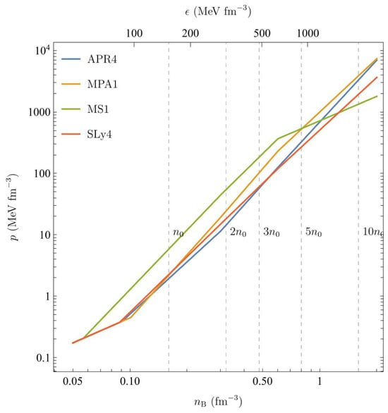
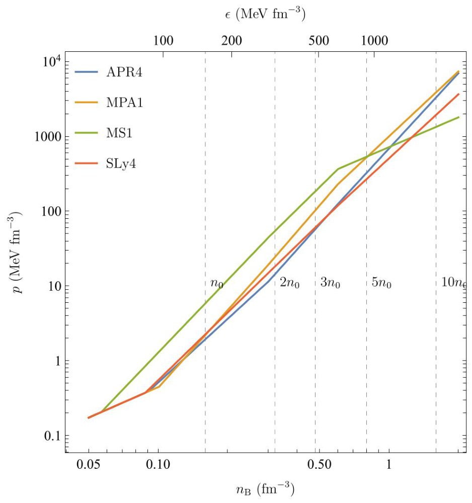
The first condition selects the radially stable branch preceding the first maximum of $M_0\left({ϵ}_c\right)$. The second requires the local adiabatic sound speed to remain causal throughout the stellar interior, with $dp/dϵ$ evaluated in the corresponding polytropic segment. Figure 1 shows the pressure–density relations of the four EoSs, while Figure 2, Figure 3 and Figure 4 illustrate the corresponding stellar equilibrium sequences. The latter are shown without imposing a causality cutoff and therefore include acausal configurations where present. By contrast, the determination of the $w_{\mathrm{HT}}=3$ configurations and the comparison with the Urbanec compactness relation are restricted to causal, radially stable models satisfying the numerical acceptance criteria.

Figure 1. Pressure p as a function of baryon number density $n_B$ for the APR4, MPA1, MS1, and SLy4 analytic EoSs. The upper axis gives the corresponding energy density using APR4 as a reference, and the vertical lines mark selected multiples of the nuclear saturation density $n_0=0.16{\mathrm{fm}}^{-3}$.

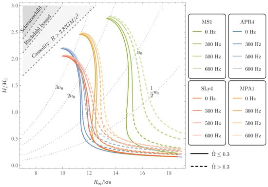
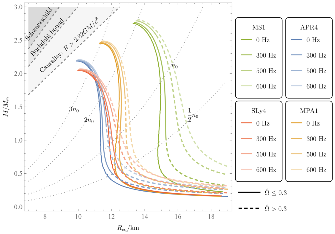
Figure 2. Mass–radius relations for the APR4, MPA1, MS1, and SLy4 EoSs at 0, 300, 500, and $600\mathrm{Hz}$ in the Hartle–Thorne approximation. For the nonrotating sequences, $M=M_0$ and $R_{\mathrm{eq}}=R_0$; for the rotating sequences, $M=M_0+\delta M$, and $R_{\mathrm{eq}}$ is the equatorial circumferential radius calculated through second order. Dashed portions at the low-mass ends of the finite-frequency sequences indicate $\widehat{\mathrm{\Omega }}>0.3$, where the adopted slow-rotation criterion is not satisfied. Solid portions include the higher-central-density continuations beyond the first mass maxima. For nonrotating configurations, the first mass maximum marks the onset of radial instability; for rotating configurations, constant-frequency mass maxima are not independently identified with stability boundaries. Both causal and acausal equilibrium configurations are shown, without separately marking the EoS-dependent causality limits. The shaded compactness bounds apply to static, spherically symmetric models and are included only for reference. Dotted curves indicate constant mass-based mean densities ${\overline{n}}_M/n_0=1/2,1,2$, and 3, with $n_0=0.16{\mathrm{fm}}^{-3}$. Only causal, radially stable nonrotating backgrounds are used in the analysis of $w_{\mathrm{HT}}=3$.

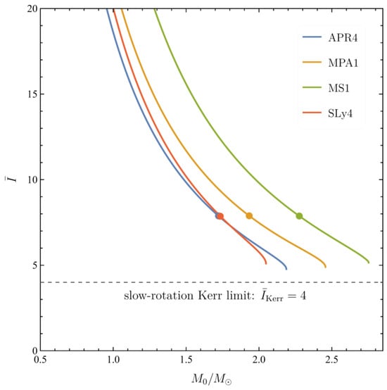
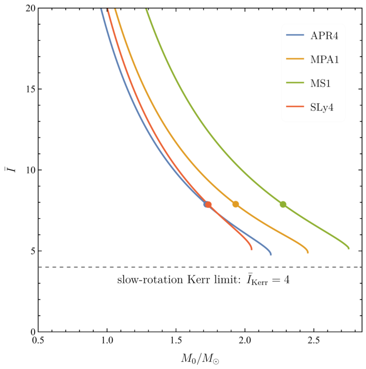
Figure 3. Dimensionless moment of inertia $\overline{I}$ as a function of the nonrotating gravitational mass $M_0$ for the APR4, MPA1, MS1, and SLy4 EoSs. Each sequence extends to its first TOV mass maximum, without a causality cut; hence the highest-density portions may contain acausal equilibrium configurations. The large colored circles identify the causal, radially stable configurations at which the directly calculated Hartle–Thorne quadrupole factor satisfies $w_{\mathrm{HT}}=3$. The horizontal dashed line at $\overline{I}=4$ denotes the slow-rotation Kerr limit.

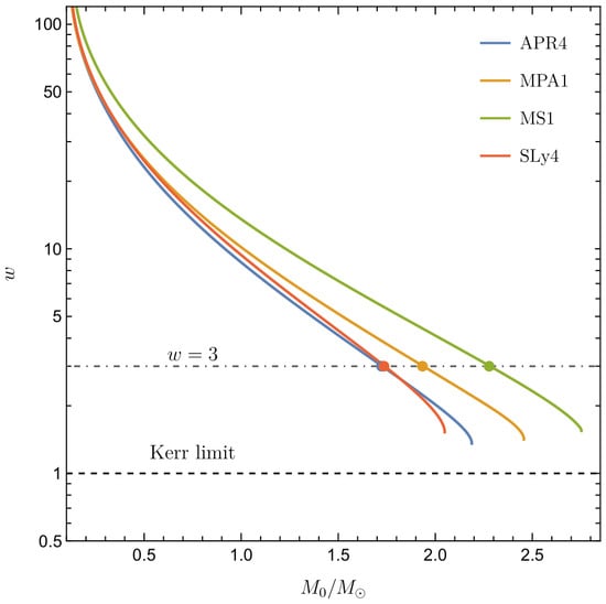
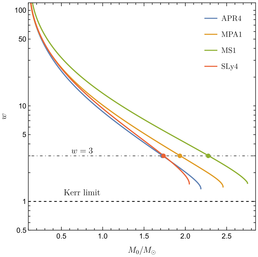
Figure 4. Hartle–Thorne quadrupole factor $w_{\mathrm{HT}}$ as a function of the nonrotating background mass $M_0$ for the APR4, MPA1, MS1, and SLy4 EoSs. The curves extend to the first TOV mass maximum without imposing a causality cut; acausal high-density configurations are included where present. The colored circles identify the causal, radially stable configurations satisfying $w_{\mathrm{HT}}=3$, associated with the quadrupole-induced spin flip–flop regime of nearly equal-mass binaries. The dash-dotted and dashed horizontal lines indicate $w_{\mathrm{HT}}=3$ and the Kerr limit $w_{\mathrm{HT}}=1$, respectively.

2.2. TOV Backgrounds and the Urbanec Compactness Relation

For each EoS shown in Figure 1 and specified in Table 1, the nonrotating stellar configurations are obtained by integrating the Tolman–Oppenheimer–Volkoff (TOV) equations,

$${\displaystyle \frac{dm}{dr}}=4\pi r^2{\displaystyle \frac{ϵ}{c^2}},$$

(8)

$${\displaystyle \frac{dp}{dr}}=-{\displaystyle \frac{G}{r^2}}\left({\displaystyle \frac{ϵ+p}{c^2}}\right){\displaystyle \frac{m+4\pi r^{3}p/c^2}{1-2Gm/\left(r{c}^2\right)}},$$

(9)

with the barotropic EoS $ϵ=ϵ\left(p\right)$ and regular central boundary conditions. For a prescribed central energy density ${ϵ}_c$, the stellar radius and gravitational mass are determined by $p\left(R_0\right)=0$ and $M_0=m\left(R_0\right)$, respectively. The corresponding compactness is

$$C_0={\displaystyle \frac{G{M}_0}{R_0{c}^2}}.$$

(10)

The equilibrium sequences are parametrized by ${ϵ}_c$. The first maximum of $M_0\left({ϵ}_c\right)$ satisfies

$${\left.{\displaystyle \frac{d{M}_0}{d{ϵ}_c}}\right|}_{{ϵ}_{c,\max }}=0.$$

(11)

The preceding branch, with $d{M}_0/d{ϵ}_c>0$, is radially stable. At the maximum, the frequency of the fundamental radial mode vanishes, and the continuation beyond this point contains one unstable radial mode [21,22].

The corresponding slowly rotating configurations are described through second order in the Hartle–Thorne expansion. Their gravitational mass and equatorial circumferential radius are denoted by

$$M=M_0+\delta M$$

(12)

and $R_{\mathrm{eq}}$, respectively. The monopole mass correction and the equatorial circumferential radius, including the rotational deformation of the stellar surface, are specified in Section 2.4. In the nonrotating limit, $M\to M_0$ and $R_{\mathrm{eq}}\to R_0$. For the mass–radius diagram, we define the mass-based mean-density quantity

$${\overline{n}}_M\equiv {\displaystyle \frac{3M}{4\pi R_{\mathrm{eq}}^3{m}_b}},$$

(13)

where $m_b$ is the reference baryon mass introduced in Equation (2). Since ${\overline{n}}_M$ is constructed from the gravitational mass, it is distinct from the volume average of the local baryon number density $n_B$.

The applicability of the slow-rotation approximation is characterized by the dimensionless parameter

$$\widehat{\mathrm{\Omega }}=\mathrm{\Omega }\sqrt{{\displaystyle \frac{R_0^3}{G{M}_0}}},$$

(14)

which must remain small. Comparisons with fully relativistic rotating-star models demonstrate the increasing importance of higher-order rotational corrections at larger rotation rates [23]. At fixed frequency, $\widehat{\mathrm{\Omega }}$ increases with $R_0^{3/2}/M_0^{1/2}$, making the approximation particularly restrictive for low-mass, large-radius configurations. In Figure 2, segments with $\widehat{\mathrm{\Omega }}>0.3$ are distinguished by dashed lines at the low-mass ends of the finite-frequency sequences. These segments represent formal continuations of the second-order solutions outside the adopted slow-rotation domain. The threshold $\widehat{\mathrm{\Omega }}=0.3$ is not a universal convergence bound and does not determine the relativistic mass-shedding limit [24].

For uniformly rotating barotropic stars, the turning-point theorem [25] provides a sufficient criterion for the onset of secular axisymmetric instability at an extremum of the gravitational mass along a sequence of constant angular momentum,

$${\left({\displaystyle \frac{\partial M}{\partial {ϵ}_c}}\right)}_J=0.$$

(15)

An equivalent turning-point condition is an extremum of the angular momentum along a sequence of constant baryon mass,

$${\left({\displaystyle \frac{\partial J}{\partial {ϵ}_c}}\right)}_{M_b}=0.$$

(16)

A mass maximum along a constant-frequency sequence does not, in general, coincide with either turning point and is therefore not independently identified with the onset of instability.

Figure 2 shows the mass–radius relations for the four EoSs at $f=0$, 300, 500, and $600\mathrm{Hz}$. Rotation increases the equatorial radius and modifies the maximum gravitational mass, while the larger radii of MS1 reflect its greater stiffness. The dotted curves indicate constant ${\overline{n}}_M$. For reference, the figure also shows the Schwarzschild radius, $R=2GM/c^2$; the Buchdahl bound, $R\ge (9/4)GM/c^2$, for static, spherically symmetric, isotropic perfect-fluid configurations [26]; and the causality bound for maximally compact stellar models, $R\gtrsim 2.82GM/c^2$ [27]. These compactness limits refer to static spherical configurations and are not imposed on the rotating sequences. The finite-frequency curves illustrate rotational modifications of the mass–radius relations. They are not used to determine the leading-order $w_{\mathrm{HT}}=3$ roots, which are obtained from causal, radially stable nonrotating backgrounds and are independent of the spin normalization at the retained perturbative order.

The compactness dependence of the quadrupole factor may be compared with the relation obtained by Urbanec, Miller, and Stuchlík [7]. Introducing

$$x={\displaystyle \frac{R_0}{2M_0}}={\displaystyle \frac{1}{2C_0}}$$

(17)

in geometrized units, their neutron-star fit takes the form

$$w_{\mathrm{U}}\left(C_0\right)=\left\{\begin{array}{cc}3.64x-5.3,\hfill & x>2.4615,\hfill \\ 1.2453{(x-1)}^2+1,\hfill & x\le 2.4615.\hfill \end{array}\right.$$

(18)

The neutron-star models considered by Urbanec et al. [7] comprise eight EoSs: A18+$\delta v$+UIX*, UBS, BBB2, SLy4, BPAL12, Gandolfi, and the hyperonic BALBN1H1 and GLENDH3; strange-star models were treated separately. The compactness variable x refers to the nonrotating stellar background. The coefficients of the quadratic branch are determined by requiring continuity of the fit and its first derivative at the matching point, together with the Kerr limit $w_{\mathrm{U}}(x=1)=1$.

The condition $w_{\mathrm{U}}\left(C_0\right)=3$ corresponds to $C_0\simeq 0.2205$. Although the Urbanec relation is approximately EoS independent, its residual EoS dependence implies that the configuration satisfying $w_{\mathrm{U}}\left(C_0\right)=3$ need not coincide with that for which the directly calculated Hartle–Thorne quadrupole factor satisfies $w_{\mathrm{HT}}=3$.

2.3. First-Order Moment of Inertia

For the rotational perturbation equations we use geometrized units and write the spherical background metric as

$$d{s}^2=-e^{2\nu \left(r\right)}d{t}^2+e^{2\lambda \left(r\right)}d{r}^2+r^2\left(d{\theta }^2+{\sin }^2\theta d{\varphi }^2\right),e^{-2\lambda \left(r\right)}=1-{\displaystyle \frac{2m\left(r\right)}{r}}.$$

(19)

For uniform rotation, the first-order Hartle equation for $\overline{\omega }=\mathrm{\Omega }-\omega$ is [28]

$${\displaystyle \frac{d}{dr}}\left(r^{4}j{\displaystyle \frac{d\overline{\omega }}{dr}}\right)+4r^3{\displaystyle \frac{dj}{dr}}\overline{\omega }=0,j=e^{-(\nu +\lambda )}.$$

(20)

Regularity at the center requires $d\overline{\omega }/dr=0$. Matching the interior solution to the exterior frame-dragging solution at $R_0$ gives

$$J={\displaystyle \frac{c^2{R}_0^4}{6G}}{\left.{\displaystyle \frac{d\overline{\omega }}{dr}}\right|}_{R_0},\mathrm{\Omega }=\overline{\omega }\left(R_0\right)+{\displaystyle \frac{2GJ}{c^2{R}_0^3}},I={\displaystyle \frac{J}{\mathrm{\Omega }}}.$$

(21)

Because Equation (20) is linear and homogeneous, the arbitrary normalization of the central value of $\overline{\omega }$ cancels in I. We further define the dimensionless moment of inertia by

$$\overline{I}\equiv {\displaystyle \frac{I}{M_0^3}}={\displaystyle \frac{c^{4}I}{G^2{M}_0^3}},$$

(22)

where the first expression applies in geometrized units and the second restores physical units.

Figure 3 shows $\overline{I}$ as a function of the nonrotating gravitational mass $M_0$ for the four EoSs. The sequences terminate at the first maximum of $M_0$, corresponding to the maximum-mass turning point of the nonrotating sequence. The dimensionless moment of inertia decreases with increasing $M_0$ along each sequence and remains above the slow-rotation Kerr value ${\overline{I}}_{\mathrm{Kerr}}=4$. The configurations satisfying the directly calculated condition $w_{\mathrm{HT}}=3$, determined in Section 3.1, are indicated by the colored circles.

For comparison with the compactness-based prediction examined below, Table 3 gives the first-order rotational quantities at the four configurations satisfying $w_{\mathrm{U}}\left(C_0\right)=3$.

Table 3. First-order rotational quantities at the configurations satisfying $w_{\mathrm{U}}\left(C_0\right)=3$. Here $I_{45}=I/\left({10}^{45}\mathrm{g}{\mathrm{cm}}^2\right)$ and $\overline{I}$ is defined by Equation (22).

EoS	${\mathit{M}}_0/{\mathit{M}}_{\odot }$	${\mathit{I}}_{45}$	$\mathit{I}/\left({\mathit{M}}_0{\mathit{R}}_0^2\right)$	$\overline{\mathit{I}}$
APR4	1.675	1.681	0.401	8.246
MPA1	1.858	2.335	0.408	8.397
MS1	2.207	3.875	0.404	8.312
SLy4	1.705	1.746	0.395	8.122

2.4. Second-Order Mass, Surface Deformation, and Quadrupole

The second-order rotational corrections are obtained from the spherically symmetric $l=0$ and quadrupolar $l=2$ sectors of the Hartle–Thorne equations. For the $l=0$ sector we integrate the mass perturbation $m_0\left(r\right)$ and the normalized pressure perturbation $p_0^{*}\left(r\right)=\delta p_0\left(r\right)/(ϵ+p)$, where $\delta p_0$ is the $O\left({\mathrm{\Omega }}^2\right)$ monopole pressure perturbation. In geometrized units, the equations are [28,29]

$${\displaystyle \frac{d{m}_0}{dr}}=4\pi r^2(ϵ+p){\displaystyle \frac{dϵ}{dp}}{p}_0^{*}+{\displaystyle \frac{r^4{j}^2}{12}}{\left({\overline{\omega }}^{\prime }\right)}^2-{\displaystyle \frac{r^3}{3}}{\left(j^2\right)}^{\prime }{\overline{\omega }}^2,$$

(23)

$$\begin{array}{c} {\displaystyle \frac{d{p}_0^{*}}{dr}}=-{\displaystyle \frac{1+8\pi r^{2}p}{{(r-2m)}^2}}{m}_0-{\displaystyle \frac{4\pi r^2(ϵ+p)}{r-2m}}{p}_0^{*}+{\displaystyle \frac{r^4{j}^2}{12(r-2m)}}{\left({\overline{\omega }}^{\prime }\right)}^2\hfill \\ +{\displaystyle \frac{1}{3}}{\displaystyle \frac{d}{dr}}\left({\displaystyle \frac{r^3{j}^2{\overline{\omega }}^2}{r-2m}}\right).\hfill \end{array}$$

(24)

Here $m\left(r\right)$ and $p\left(r\right)$ are the nonrotating TOV profiles, while j and $\overline{\omega }$ are defined in Equation (20). We impose $m_0\left(0\right)=p_0^{*}\left(0\right)=0$, corresponding to perturbations at fixed central energy density. Matching the monopole perturbation to the asymptotically flat vacuum solution gives

$$\delta M=m_0\left(R_0\right)+{\displaystyle \frac{J^2}{R_0^3}}.$$

(25)

This surface expression applies to the present polytropic EoSs, for which the energy density vanishes with the pressure at $R_0$.

The spin-induced mass quadrupole is determined by the even-parity $l=2$ Hartle–Thorne sector at $O\left({\mathrm{\Omega }}^2\right)$ [28,29,30]. We integrate this sector together with the first-order frame-dragging solution and define

$$v_2=h_2+k_2.$$

(26)

The interior equations are

$${\displaystyle \frac{d{v}_2}{dr}}=-2{\nu }^{\prime }{h}_2+\left({\displaystyle \frac{1}{r}}+{\nu }^{\prime }\right)\left[{\displaystyle \frac{r^4{j}^2}{6}}{\left({\overline{\omega }}^{\prime }\right)}^2-{\displaystyle \frac{r^3{\overline{\omega }}^2}{3}}{\left(j^2\right)}^{\prime }\right],$$

(27)

$$\begin{array}{c} {\displaystyle \frac{d{h}_2}{dr}}=-{\displaystyle \frac{2v_2}{r(r-2m){\nu }^{\prime }}}-2{\nu }^{\prime }{h}_2+{\displaystyle \frac{r}{2(r-2m){\nu }^{\prime }}}\left[8\pi (ϵ+p)-{\displaystyle \frac{4m}{r^3}}\right]h_2\hfill \\ +{\displaystyle \frac{1}{6}}\left[r{\nu }^{\prime }-{\displaystyle \frac{1}{2(r-2m){\nu }^{\prime }}}\right]r^3{j}^2{\left({\overline{\omega }}^{\prime }\right)}^2-{\displaystyle \frac{1}{3}}\left[r{\nu }^{\prime }+{\displaystyle \frac{1}{2(r-2m){\nu }^{\prime }}}\right]r^2{\overline{\omega }}^2{\left(j^2\right)}^{\prime }.\hfill \end{array}$$

(28)

To construct the regular interior solution, we integrate a rotation-induced particular solution $(h_2^{\mathrm{P}},v_2^{\mathrm{P}})$ and a linearly independent homogeneous solution $(h_2^{\mathrm{H}},v_2^{\mathrm{H}})$, writing

$$h_2=h_2^{\mathrm{P}}+A{h}_2^{\mathrm{H}},v_2=v_2^{\mathrm{P}}+A{v}_2^{\mathrm{H}}.$$

(29)

At a small initial radius $r_i>0$, the regular central expansions are used to initialize the particular and homogeneous solutions:

$$\begin{array}{cccc}\hfill h_2^{\mathrm{P}}\left(r_i\right)& =0,\hfill & \hfill v_2^{\mathrm{P}}\left(r_i\right)& ={\displaystyle \frac{2\pi }{3}}({ϵ}_c+p_c){\left(j_c{\overline{\omega }}_c\right)}^2{r}_i^4,\hfill \\ \hfill h_2^{\mathrm{H}}\left(r_i\right)& =B{r}_i^2,\hfill & \hfill v_2^{\mathrm{H}}\left(r_i\right)& =-2\pi \left(p_c+{\displaystyle \frac{{ϵ}_c}{3}}\right)B{r}_i^4.\hfill \end{array}$$

(30)

Here $j_c=j\left(0\right)$ and ${\overline{\omega }}_c=\overline{\omega }\left(0\right)$.

The nonzero constant B fixes the normalization of the homogeneous solution and is absorbed into the matching coefficient A. The integration starts at $r_i=0.1\mathrm{m}$, with $B=-{\left(1\mathrm{km}\right)}^{-2}$. An auxiliary normalization $j_c=1$ is used for the numerical integration, with the physical normalization restored by matching to the exterior solution. The coefficients A and K are determined by matching the interior solutions for $h_2$ and $v_2$ continuously to the asymptotically flat exterior Hartle–Thorne solution at $r=R_0$,

$$h_2^{\mathrm{ext}}=J^2\left({\displaystyle \frac{1}{M_0{r}^3}}+{\displaystyle \frac{1}{r^4}}\right)+K{Q}_2^2\left({\displaystyle \frac{r}{M_0}}-1\right),$$

(31)

$$v_2^{\mathrm{ext}}=-{\displaystyle \frac{J^2}{r^4}}+K{\displaystyle \frac{2M_0}{\sqrt{r(r-2M_0)}}}{Q}_2^1\left({\displaystyle \frac{r}{M_0}}-1\right).$$

(32)

Here, $Q_2^1$ and $Q_2^2$ are associated Legendre functions of the second kind. For $x=r/M_0-1>1$, we adopt the Hartle convention

$$\begin{array}{cc}\hfill Q_2\left(x\right)& ={\displaystyle \frac{1}{4}}(3x^2-1)\ln {\displaystyle \frac{x+1}{x-1}}-{\displaystyle \frac{3}{2}}x,\hfill \\ \hfill Q_2^1\left(x\right)& =-\sqrt{x^2-1}{\displaystyle \frac{d{Q}_2}{dx}},\hfill \\ \hfill Q_2^2\left(x\right)& =(x^2-1){\displaystyle \frac{d^2{Q}_2}{d{x}^2}}.\hfill \end{array}$$

(33)

With these definitions, both $Q_2^1$ and $Q_2^2$ are positive for $x>1$. The exterior matching coefficient K determines the signed mass quadrupole moment Q and the dimensionless factor $w_{\mathrm{HT}}$,

$$Q=-{\displaystyle \frac{J^2}{M_0}}-{\displaystyle \frac{8}{5}}K{M}_0^3,w_{\mathrm{HT}}=-{\displaystyle \frac{Q{M}_0}{J^2}}=1+{\displaystyle \frac{8}{5}}{\displaystyle \frac{K{M}_0^4}{J^2}}.$$

(34)

The displacement of the stellar surface in the Hartle radial gauge is

$$r_{\mathrm{s}}\left(\theta \right)=R_0+{\xi }_0\left(R_0\right)+{\xi }_2\left(R_0\right)P_2\left(\cos \theta \right),P_2\left(\cos \theta \right)=\frac{1}{2}(3{\cos }^2\theta -1),$$

(35)

where the displacement functions follow from the pressure perturbations and the background hydrostatic equation:

$${\xi }_0\left(R_0\right)={\displaystyle \frac{p_0^{*}\left(R_0\right)}{{\nu }^{\prime }\left(R_0\right)}},$$

(36)

$${\xi }_2\left(R_0\right)=-{\displaystyle \frac{1}{{\nu }^{\prime }\left(R_0\right)}}\left[h_2\left(R_0\right)+{\displaystyle \frac{R_0^2}{3}}{e}^{-2\nu \left(R_0\right)}{\overline{\omega }}^2\left(R_0\right)\right],$$

(37)

with ${\nu }^{\prime }\left(R_0\right)=M_0/\left[R_0(R_0-2M_0)\right]$ for a zero-pressure surface. In the Hartle gauge, with the monopole angular perturbation set to zero, $k_0=0$, the azimuthal metric component is $g_{\varphi \varphi }=r^2[1+2k_2\left(r\right)P_2\left(\cos \theta \right)]{\sin }^2\theta$, where $k_2=v_2-h_2$. The equatorial circumferential radius is therefore

$$R_{\mathrm{eq}}=\sqrt{g_{\varphi \varphi }(r_{\mathrm{s}}(\pi /2),\pi /2)}=R_0+{\xi }_0\left(R_0\right)-{\displaystyle \frac{1}{2}}{\xi }_2\left(R_0\right)-{\displaystyle \frac{R_0}{2}}{k}_2\left(R_0\right)+O\left({\mathrm{\Omega }}^4\right).$$

(38)

Thus, the equatorial radius includes both the displacement of the surface and the second-order angular-metric perturbation. All the quantities entering Equations (25) and (38) are evaluated on the same nonrotating background.

Since $J=O\left(\mathrm{\Omega }\right)$, $Q=O\left({\mathrm{\Omega }}^2\right)$, and $M=M_0+O\left({\mathrm{\Omega }}^2\right)$, the mass entering $w_{\mathrm{HT}}$ at the perturbative order considered here is the background mass $M_0$. Replacing it by the rotation-corrected gravitational mass would modify the dimensionless quadrupole factor only beyond the consistently retained order. Consequently, $w_{\mathrm{HT}}$ and the background configuration corresponding to a specified value of $w_{\mathrm{HT}}$ are invariant under the arbitrary normalization of the slow-rotation parameter at this order, whereas the dimensional quadrupole moment Q scales quadratically with any chosen sufficiently small reference frequency. Rotation-dependent normalizations involving either the TOV mass or the rotation-corrected gravitational mass are discussed in the context of I–Love–Q–$\delta M$ relations [31].

2.5. Numerical Root Determination and Validation

After bracketing a sign change of $w_{\mathrm{HT}}-3$ along each nonrotating TOV sequence, we determine the root in central pressure, equivalently in central energy density, by repeating the TOV, first-order, and $l=2$ Hartle–Thorne integrations at each trial configuration. For the four EoSs, the residuals of the roots determined with the numerical settings described below satisfy $|w_{\mathrm{HT}}-3|<2\times {10}^{-10}$. This residual measures the numerical closure of the root search; it does not represent the uncertainty associated with the EoS representation or with truncation of the slow-rotation expansion. The properties of the roots are listed in Table 4, with masses rounded to three decimal places in the discussion.

Table 4. Properties of the stellar configurations satisfying the directly calculated condition $w_{\mathrm{HT}}=3$. The dimensionless moment of inertia ${\overline{I}}_{\mathrm{HT}}$ is defined by Equation (22).

EoS	${\mathit{ϵ}}_{\mathit{c},\mathit{w}=3}\left[\mathbf{MeV}{\mathbf{fm}}^{-3}\right]$	${\mathit{p}}_{\mathit{c},\mathit{w}=3}\left[\mathbf{MeV}{\mathbf{fm}}^{-3}\right]$	${\mathit{M}}_{\mathbf{HT}}/{\mathit{M}}_{\odot }$	${\overline{\mathit{I}}}_{\mathbf{HT}}$
APR4	699.416	170.145	1.727	7.848
MPA1	542.567	132.891	1.938	7.855
MS1	418.860	100.118	2.283	7.839
SLy4	747.233	177.252	1.739	7.826

The rotational perturbation equations are integrated adaptively from regular central data and matched to the exterior Hartle–Thorne solution near the stellar surface. Numerical convergence was examined at the four configurations satisfying $w_{\mathrm{HT}}\simeq 3$. We varied the maximum radial integration step over 25, 50, and 100 m while keeping the relative integration tolerance fixed at $2\times {10}^{-9}$, the surface-pressure cutoff at ${10}^{-10}\mathrm{MeV}{\mathrm{fm}}^{-3}$, and the reference spin frequency at 300 Hz. Across the four EoSs, the largest relative change in $w_{\mathrm{HT}}$ was $7.4\times {10}^{-12}$. Independently refining the $w_{\mathrm{HT}}=3$ root at each of the three maximum step sizes yielded a maximum spread of $7.3\times {10}^{-12}{M}_{\odot }$ in the crossing mass. At a maximum step of 25 m, tightening the relative integration tolerance to $5\times {10}^{-10}$ changed $w_{\mathrm{HT}}$ by at most $5.4\times {10}^{-14}$ relative. Varying the surface-pressure cutoff between ${10}^{-9}$ and ${10}^{-11}\mathrm{MeV}{\mathrm{fm}}^{-3}$ changed $w_{\mathrm{HT}}$ by at most $9.8\times {10}^{-12}$ relative. These comparisons measure the sensitivity to the stated numerical controls for the four crossing configurations; they do not independently bound common systematic errors in the integration or exterior matching procedure.

The normalization of the first- and second-order rotational perturbations was checked at reference frequencies of 50, 200, 300, and 600 Hz, using the same four nonrotating backgrounds. The maximum relative variations in $w_{\mathrm{HT}}$, $J/f$, and $Q/f^2$ were $3.1\times {10}^{-13}$, $4.9\times {10}^{-13}$, and $4.5\times {10}^{-13}$, respectively. These results are consistent with the first- and second-order scalings $J\propto \mathrm{\Omega }$ and $Q\propto {\mathrm{\Omega }}^2$ and provide a check of the numerical implementation. Invariance under rescaling of the reference frequency does not, by itself, establish the accuracy of the slow-rotation approximation for physical stars rotating at 600 Hz.

Two comparisons with independent published results further test the implementation. At $M_0=1.338M_{\odot }$, the first-order moments of inertia agree with the values reported by Read et al. to within $0.8\%$ [18]. The complete $l=2$ solver reproduces the homogeneous-star Hartle quadrupole factors tabulated by Posada with a maximum relative discrepancy of $3.3\times {10}^{-4}$ over the six tested compactness parameters $\zeta =R/\left(2M\right)-1=0.5,1,2,3,9,99$ in that reference’s notation [30]. These benchmark comparisons and the convergence tests address numerical consistency within the adopted model; they do not quantify the uncertainty arising from the analytic EoS approximations or from neglected higher-order rotational terms.

The applicability of the second-order approximation to the illustrative finite-frequency sequences was further examined using the dimensionless rotation parameter defined in Equation (14). The accompanying HT_figures_slowrotation directory and its HT_slow_rotation_audit.csv file document the application of the adopted criterion $\widehat{\mathrm{\Omega }}\le 0.30$ to each EoS and frequency. Among the causal, radially stable configurations satisfying the numerical background-agreement criteria and this rotation threshold, the maximum fractional second-order mass and equatorial-radius corrections are $|\delta M|/M_0=0.0316$ and $|R_{\mathrm{eq}}-R_0|/R_0=0.0320$, respectively. At $600\mathrm{Hz}$, none of the examined MS1 configurations satisfies the adopted threshold. In Figure 2, portions exceeding this threshold are distinguished by dashed lines. These diagnostics characterize the magnitude of the retained rotational corrections but do not provide an independent estimate of the omitted higher-order terms or determine the relativistic mass-shedding limit. The accompanying numerical files also include the source code and model-level diagnostics required to reproduce the calculations. The unrounded seven-segment EoS parameters, physical constants, and unit conversion factors are provided as described in Section 2.1.

3. Results

3.1. Direct $w_{\mathrm{HT}}=3$ Configurations

The Urbanec relation, Equation (18), yields $w_{\mathrm{U}}\left(C_0\right)=3$ at background masses $M_{\mathrm{U}}=1.675$, $1.858$, $2.207$, and $1.705M_{\odot }$ for APR4, MPA1, MS1, and SLy4, respectively. Direct evaluation of the Hartle–Thorne quadrupole factor from Equation (34) at these configurations gives $w_{\mathrm{HT}}=3.225$, $3.305$, $3.266$, and $3.167$, respectively. Thus, for all four EoSs, the configurations selected by $w_{\mathrm{U}}\left(C_0\right)=3$ have directly calculated quadrupole factors $w_{\mathrm{HT}}>3$. The direct condition $w_{\mathrm{HT}}=3$ is satisfied at background masses $M_{\mathrm{HT}}=1.727$, $1.938$, $2.283$, and $1.739M_{\odot }$ for APR4, MPA1, MS1, and SLy4, respectively. The corresponding differences between the direct and compactness-based crossing masses are $M_{\mathrm{HT}}-M_{\mathrm{U}}=0.052$, $0.080$, $0.076$, and $0.034M_{\odot }$.

The corresponding masses are compared with those inferred from the Urbanec compactness relation in Table 5, where $M_{\mathrm{U}}$ denotes the background mass satisfying $w_{\mathrm{U}}\left(C_0\right)=3$ and $M_{\mathrm{HT}}$ the direct root of $w_{\mathrm{HT}}=3$.

Table 5. Comparison between the masses corresponding to $w_{\mathrm{U}}\left(C_0\right)=3$ and the directly calculated condition $w_{\mathrm{HT}}=3$.

EoS	${\mathit{M}}_{\mathbf{U}}/{\mathit{M}}_{\odot }$	${\mathit{w}}_{\mathbf{HT}}\left({\mathit{M}}_{\mathbf{U}}\right)$	${\mathit{M}}_{\mathbf{HT}}/{\mathit{M}}_{\odot }$	$\mathbf{\Delta }\mathit{M}/{\mathit{M}}_{\odot }$	${\mathit{\delta }}_{\mathit{w}}\left({\mathit{M}}_{\mathbf{U}}\right)$
APR4	1.675	3.225	1.727	0.052	0.075
MPA1	1.858	3.305	1.938	0.080	0.102
MS1	2.207	3.266	2.283	0.076	0.089
SLy4	1.705	3.167	1.739	0.034	0.056

The mass dependence of the directly calculated quadrupole factor is shown in Figure 4. For all four EoSs, $w_{\mathrm{HT}}$ decreases monotonically with increasing $M_0$ over the sequences considered and remains above the Kerr value $w_{\mathrm{HT}}=1$. The condition $w_{\mathrm{HT}}=3$ is attained within the causal, radially stable branch of each sequence, at an EoS-dependent value of $M_0$ indicated by the colored circles.

For all four EoSs, the direct $w_{\mathrm{HT}}=3$ crossing occurs at a larger mass than that inferred from $w_{\mathrm{U}}\left(C_0\right)=3$, with $M_{\mathrm{HT}}-M_{\mathrm{U}}=0.034$–$0.080M_{\odot }$. These offsets exceed the maximum spread of $7.3\times {10}^{-12}{M}_{\odot }$ in the $w_{\mathrm{HT}}=3$ crossing masses obtained by varying the maximum radial integration step between 25 and $100\mathrm{m}$ (see Section 2.5). They therefore cannot be attributed to the numerical variations measured in this convergence test. The mass differences reflect the systematic offset between the Urbanec relation and the direct Hartle–Thorne results near $w=3$, together with the EoS-dependent relation between compactness and stellar mass.

3.2. Quadrupole–Compactness Relation

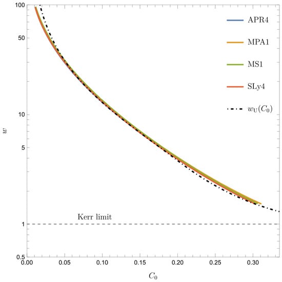
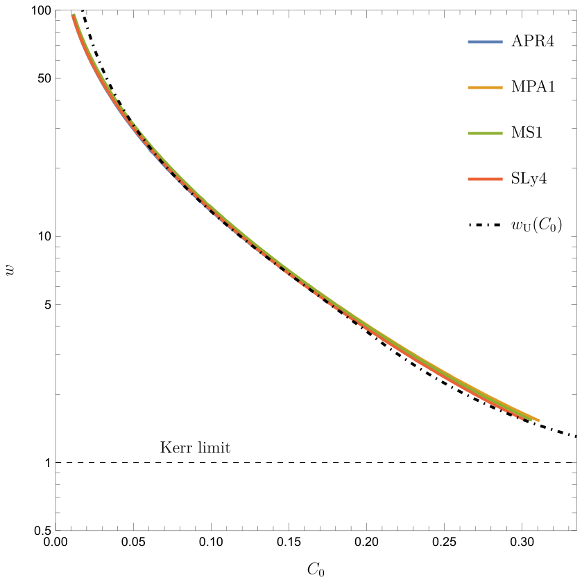
Figure 5 shows the dependence of the quadrupole factor on the background compactness $C_0$ defined by Equation (10). For all four EoSs, $w_{\mathrm{HT}}$ decreases monotonically with increasing $C_0$ along the causal, radially stable sequences and remains above the Kerr value $w=1$. At fixed compactness, the EoS dependence of $w_{\mathrm{HT}}$ is comparatively weak relative to its overall variation with $C_0$, although residual differences remain. The Urbanec relation $w_{\mathrm{U}}\left(C_0\right)$ reproduces the general compactness dependence of the directly calculated quadrupole factor.

Figure 5. Dimensionless quadrupole factor w as a function of the nonrotating background compactness $C_0=G{M}_0/\left(R_0{c}^2\right)$ for the APR4, MPA1, MS1, and SLy4 EoSs. The colored solid curves give the directly calculated Hartle–Thorne factor $w_{\mathrm{HT}}$, restricted to causal, radially stable and numerically accepted configurations. Their upper compactness endpoints therefore differ among the EoSs. The black dot-dashed curve is the Urbanec relation $w_{\mathrm{U}}\left(C_0\right)$, and the horizontal dashed line indicates the Kerr limit $w=1$.

The Urbanec condition $w_{\mathrm{U}}\left(C_0\right)=3$ occurs at $C_0\simeq 0.2205$, whereas the direct condition $w_{\mathrm{HT}}=3$ is attained at an EoS-dependent compactness. To quantify the departure from the Urbanec relation, we define

$$\Delta w=w_{\mathrm{HT}}-w_{\mathrm{U}}\left(C_0\right),{\delta }_w={\displaystyle \frac{w_{\mathrm{HT}}-w_{\mathrm{U}}\left(C_0\right)}{w_{\mathrm{U}}\left(C_0\right)}}.$$

(39)

Positive values of $\Delta w$ and ${\delta }_w$ indicate that the directly calculated Hartle–Thorne quadrupole factor exceeds the Urbanec prediction, while negative values indicate the opposite.

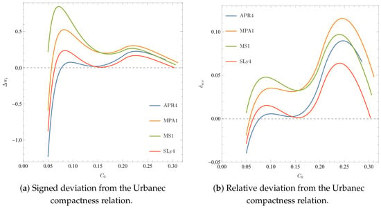
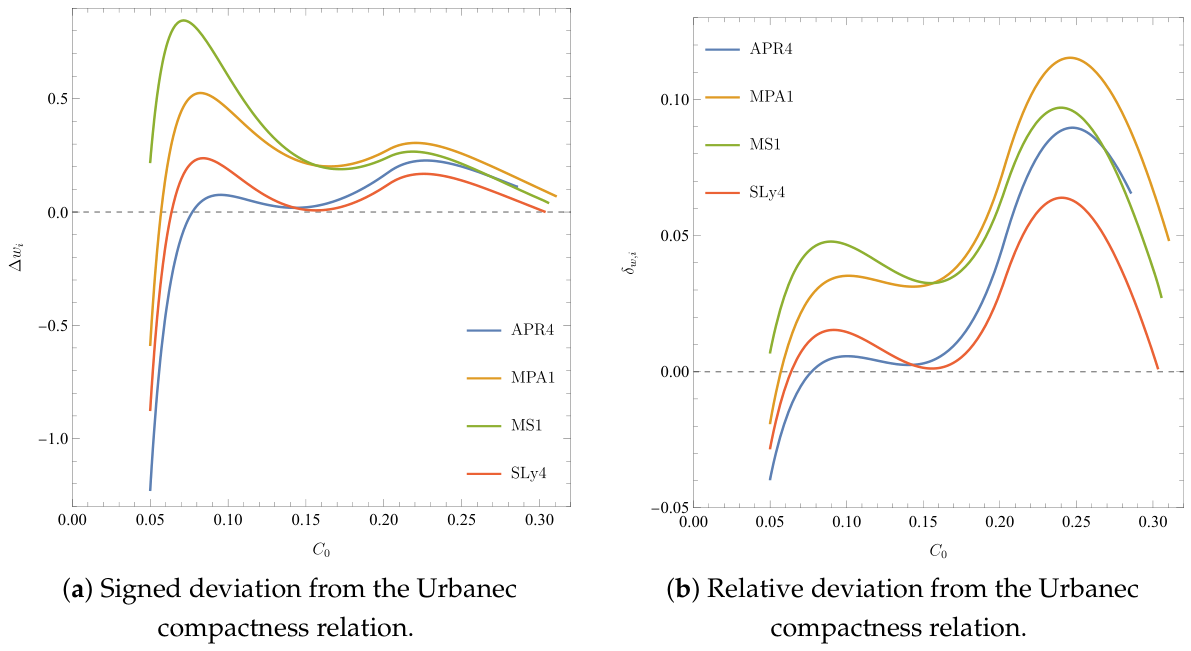
The residuals are shown in Figure 6. They vary nonmonotonically with compactness, with an EoS-dependent amplitude and sign. For each EoS, the interval $0.05\le C_0\le 0.32$ is restricted to the causal, radially stable configurations satisfying the numerical background-agreement criterion. The resulting upper compactness limits are $0.2855$, $0.3103$, $0.3055$, and $0.3031$ for APR4, MPA1, MS1, and SLy4, respectively. Thus, the accepted APR4 and MPA1 sequences terminate at the causality limit before reaching the first TOV mass maximum. At low compactness, $\Delta w$ is negative for APR4, MPA1, and SLy4, so that the Urbanec relation overestimates the directly calculated quadrupole factor there, whereas the MS1 residual remains positive over the domain considered. Evaluating shape-preserving cubic interpolants of the accepted sequences on a uniform grid of ${10}^4$ intervals in $C_0$ for each EoS gives minimum and maximum values of $\Delta w$ of approximately $(-1.251,0.229)$ for APR4, $(-0.652,0.515)$ for MPA1, $(0.042,0.834)$ for MS1, and $(-0.930,0.238)$ for SLy4. The corresponding extrema of ${\delta }_w$ are $(-4.0\%,9.0\%)$, $(-2.1\%,11.6\%)$, $(0.6\%,9.7\%)$, and $(-3.0\%,6.5\%)$, respectively. These extrema refer to the stated EoS-dependent intervals; in particular, the negative minima for APR4, MPA1, and SLy4 occur at the lower plotting limit $C_0=0.05$.

Figure 6. Deviations of the directly calculated Hartle–Thorne quadrupole factor $w_{\mathrm{HT}}$ from the Urbanec compactness relation $w_{\mathrm{U}}\left(C_0\right)$ for the APR4, MPA1, MS1, and SLy4 EoSs, as functions of the nonrotating background compactness $C_0=G{M}_0/\left(R_0{c}^2\right)$. Panel (a) shows the signed deviation $\Delta w$, and panel (b) the relative deviation ${\delta }_w$, both defined in Equation (39). For each EoS, the curves are restricted to the intersection of $0.05\le C_0\le 0.32$ with the causal, radially stable and numerically accepted configurations; their upper endpoints therefore differ. The horizontal dotted lines indicate zero deviation.

At $C_0=C_{\mathrm{U}}\simeq 0.2205$, where $w_{\mathrm{U}}\left(C_{\mathrm{U}}\right)=3$, the direct calculations at the configurations reported in Table 5 give relative deviations of $7.5\%$, $10.2\%$, $8.9\%$, and $5.6\%$ for APR4, MPA1, MS1, and SLy4, respectively. These deviations are evaluated at the common compactness $C_0=C_{\mathrm{U}}$ and are distinct from the maxima of ${\delta }_w\left(C_0\right)$ along the individual stellar sequences reported above. The mean of the four direct quadrupole factors is $⟨w_{\mathrm{HT}}⟩=3.24075$, corresponding to an average excess of $8.0\%$ over the Urbanec prediction. By comparison, the full range of the direct values is $0.138$, or $4.3\%$ of their mean. Thus, at this compactness, the mean offset from the Urbanec fit exceeds the EoS-dependent spread among the four models. This distinction does not imply a breakdown of the approximate universality of the quadrupole–compactness relation. Nor does the positive offset at $C_{\mathrm{U}}$ establish its sign for other EoSs or at arbitrary compactness. Indeed, the signed residuals in Figure 6 vary nonmonotonically with compactness and change sign for three of the four EoSs over the investigated domain, precluding a single compactness-independent correction.

4. Discussion

All four EoSs contain causal, radially stable configurations with $w_{\mathrm{HT}}=3$, the characteristic quadrupole factor associated with large-amplitude quadrupole-induced spin flip–flops in nearly equal-mass binaries. The role of $w\simeq 3$ in the spin dynamics follows from Ref. [3]. For equal masses and a dominant first spin (${\chi }_2\ll {\chi }_1$), the spin-precession coefficients satisfy

$$\left|{\displaystyle \frac{A_{S_1}}{B_{S_1}}}\right|=\left|{\displaystyle \frac{3-w_1-w_1{x}_1\cos {\kappa }_1}{2-w_1{x}_1\cos {\kappa }_1}}\cot {\kappa }_1\right|,$$

(40)

where $x_1={\chi }_1/{\overline{l}}_r$, ${\overline{l}}_r$ is the orbit-averaged dimensionless orbital angular momentum, and ${\kappa }_1$ is the inclination of the dominant spin relative to the orbital angular momentum. Large spin reorientations are favored when $|A_{S_1}|\ll |B_{S_1}|$. Since the largest attainable change of the polar angle of the smaller spin is $2\arctan |B_{S_1}/A_{S_1}|$ [Equation (64) of Ref. [3]], a flip–flop amplitude of at least $\mathrm{\Theta }$ requires, to leading order in $x_1$,

$$|w_1-3|\lesssim 2|\tan {\kappa }_1|\cot {\displaystyle \frac{\mathrm{\Theta }}{2}}.$$

(41)

For $\mathrm{\Theta }={170}^{\circ }$, this gives $|w_1-3|\lesssim 0.10$ at ${\kappa }_1={30}^{\circ }$ and $|w_1-3|\lesssim 0.18$ at ${\kappa }_1={45}^{\circ }$, whereas for ${\kappa }_1$ close to ${90}^{\circ }$ large flip–flops occur for any $w_1$. The admissible range of $w_1$ therefore depends on the orbital and spin parameters. For unequal masses, the coefficient $A_{S_1}$ also contains the term $\nu -{\nu }^{-1}$, with $\nu =m_2/m_1$, which is not suppressed by the factor $x_1$ [3]. The quadrupole-induced flip–flop near $w=3$ therefore requires nearly equal component masses, with $|1-\nu |$ at most of order $x_1$; the companion of a star with $w_{\mathrm{HT}}=3$ must then have a mass close to $M_{\mathrm{HT}}$. Consequently, the width of the spin flip–flop regime depends on the binary configuration [3,4]. For a prescribed quadrupole-parameter half-width $\Delta w_{\mathrm{ff}}$ around $w=3$, the corresponding local stellar-mass half-width is

$$\Delta M_{0,\mathrm{ff}}\simeq {\displaystyle \frac{\Delta w_{\mathrm{ff}}}{{\left|d{w}_{\mathrm{HT}}/d{M}_0\right|}_{M_{\mathrm{HT}}}}},$$

(42)

provided that the derivative is nonzero and the interval is sufficiently narrow for a linear approximation. The derivative is determined by the stellar sequence, whereas $\Delta w_{\mathrm{ff}}$ depends on the binary spin dynamics and cannot be specified universally. Approximating $|d{w}_{\mathrm{HT}}/d{M}_0|$ by finite differences between the direct and Urbanec-selected configurations in Table 5 gives $4.35$, $3.80$, $3.53$, and $4.85M_{\odot }^{-1}$ for APR4, MPA1, MS1, and SLy4, respectively, so that $\Delta w_{\mathrm{ff}}=0.1$ corresponds to $\Delta M_{0,\mathrm{ff}}\simeq 0.021$–$0.028M_{\odot }$. The differences $M_{\mathrm{HT}}-M_{\mathrm{U}}$ reported in Section 3.1 measure the displacement between the direct Hartle–Thorne and Urbanec estimates of the $w=3$ crossing, rather than the physical width of the spin flip–flop regime; they are physically relevant whenever $\Delta w_{\mathrm{ff}}$ is smaller than $w_{\mathrm{HT}}\left(M_{\mathrm{U}}\right)-3=0.167$–$0.305$. For a fixed companion mass, the mass ratio also varies with $M_0$; the above conversion therefore does not by itself determine the extent of the dynamical regime. For illustration, a $1.4M_{\odot }$ companion to a star satisfying $w_{\mathrm{HT}}=3$ gives mass ratios $q=m_2/m_1=0.811$, $0.722$, $0.613$, and $0.805$ for APR4, MPA1, MS1, and SLy4, respectively. These values specify illustrative binary mass combinations, not boundaries of a dynamical spin flip–flop regime.

Table 5 compares the direct Hartle–Thorne calculation with the Urbanec compactness relation at $C_0=C_{\mathrm{U}}\simeq 0.2205$, where $w_{\mathrm{U}}\left(C_{\mathrm{U}}\right)=3$. At this compactness, the directly calculated factors are $w_{\mathrm{HT}}=3.225$, $3.305$, $3.266$, and $3.167$ for APR4, MPA1, MS1, and SLy4, respectively, exceeding the Urbanec prediction by $5.6$–$10.2\%$. Their mean is $3.24075$, corresponding to an average offset of $8.0\%$ from the fit, whereas their full range is $0.138$, or $4.3\%$ of the mean. Thus, for the four EoSs considered, the common offset from the Urbanec fit near $w=3$ is larger than the EoS-dependent spread at fixed compactness. The direct $w_{\mathrm{HT}}=3$ crossings occur at higher background masses than those inferred from $w_{\mathrm{U}}\left(C_0\right)=3$, with $M_{\mathrm{HT}}-M_{\mathrm{U}}=0.034$–$0.080M_{\odot }$. These mass differences depend on both the deviation from the compactness fit and the EoS-dependent relation between compactness and stellar mass.

Figure 6 shows that the difference between $w_{\mathrm{HT}}$ and $w_{\mathrm{U}}\left(C_0\right)$ varies with compactness. The signed residual changes sign within the investigated causal, radially stable domain for APR4, MPA1, and SLy4, while both the signed and relative residuals vary nonmonotonically. The positive difference at $C_{\mathrm{U}}$ therefore does not persist throughout the entire compactness interval. Although the Urbanec relation reproduces the overall compactness dependence of the quadrupole factor, its residual error depends on compactness and the EoS. In particular, the common positive offset at $C_{\mathrm{U}}$ does not imply a positive deviation at arbitrary compactness or for other EoSs.

For comparison with another universal relation, we consider the I–Q fit of Yagi and Yunes [8]. In our notation, their neutron-star relation is

$$\ln {\overline{I}}_{\mathrm{YY}}=1.35+0.697z-0.143z^2+0.0994z^3-0.0124z^4,z=\ln w_{\mathrm{YY}}.$$

(43)

Inverting this relation using the moments of inertia at the directly calculated $w_{\mathrm{HT}}=3$ configurations in Table 4 gives $w_{\mathrm{YY}}=3.015$, $3.019$, $3.010$, and $3.003$ for APR4, MPA1, MS1, and SLy4, respectively. The corresponding differences from $w_{\mathrm{HT}}=3$ are $0.50\%$, $0.63\%$, $0.33\%$, and $0.08\%$, evaluated before rounding. The I–Q relation therefore agrees closely with the direct quadrupole factors at the $w_{\mathrm{HT}}=3$ configurations, in contrast to the larger differences found for the Urbanec compactness relation at $C_{\mathrm{U}}$. These comparisons are evaluated at their respective reference configurations, not point by point at identical stellar masses. They show that the observed offset is not common to both relations, although they do not separately identify the contributions from their calibration procedures and the adopted EoS representations.

The numerical crossing masses depend on the adopted analytic EoS representations, including the common four-piece SLy crust and its matching to the high-density core. To quantify the sensitivity to this construction, we compared the adopted four-piece crust with a simplified model in which its highest-density polytropic segment is extended to the stellar surface. Replacing the simplified single-segment crust with the four-piece crust increases the radius at $1.4M_{\odot }$ by $0.225$–$0.483\mathrm{km}$ for the four EoSs and decreases $w_{\mathrm{HT}}$ at the fixed compactness $C_0=C_{\mathrm{U}}\simeq 0.2205$ by $4.0$–$4.2\%$. The directly determined $w_{\mathrm{HT}}=3$ crossing masses decrease by $0.0092$–$0.0127M_{\odot }$, while the corresponding mass offsets $M_{\mathrm{HT}}-M_{\mathrm{U}}$ decrease from $0.062$–$0.115M_{\odot }$ to $0.034$–$0.080M_{\odot }$. The change in $w_{\mathrm{HT}}\left(C_{\mathrm{U}}\right)$ is comparable to the $4.3\%$ full range among the four EoSs at the same compactness.

These differences characterize the sensitivity to the complete piecewise-polytropic EoS construction, rather than an isolated contribution of the outer crust. Extending the highest-density crust segment to zero density also changes the energy-density integration constants entering the core EoS. The comparison therefore does not provide a separate estimate of the crust contribution at fixed core EoS. The effects of other crust prescriptions and of replacing the analytic representations with the original tabulated microphysical EoSs have not been quantified.

The leading-order $w_{\mathrm{HT}}=3$ roots are determined from nonrotating backgrounds using the first-order frame-dragging and second-order $l=2$ Hartle–Thorne equations. The $l=0$ mass correction and rotational surface deformation enter the finite-frequency mass–radius sequences but do not affect these roots at the retained order. Post-maximum configurations are excluded from the root determination by Equation (7).

The convergence tests in Section 2.5 give a maximum relative variation of $7.4\times {10}^{-12}$ in $w_{\mathrm{HT}}$ and a maximum spread of $7.3\times {10}^{-12}{M}_{\odot }$ in the directly determined crossing masses when varying the maximum radial integration step. Changes in the ODE tolerance and surface-pressure threshold produce relative variations in $w_{\mathrm{HT}}$ of at most $5.4\times {10}^{-14}$ and $9.8\times {10}^{-12}$, respectively. Comparisons with published moments of inertia and homogeneous-star quadrupoles give maximum discrepancies of $0.8\%$ and $3.3\times {10}^{-4}$, respectively, providing independent checks of the first- and second-order rotational calculations. These results establish numerical convergence under the stated parameter variations and agreement with reference calculations, but do not bound the total systematic uncertainty. In particular, the $0.0092$–$0.0127M_{\odot }$ variations obtained from the two crust constructions reflect changes in the EoS model, not numerical integration errors.

At finite spin, the distinction between the leading-order quadrupole factor and the full spin-dependent quadrupole ratio becomes relevant. With $J=J_1\mathrm{\Omega }+J_3{\mathrm{\Omega }}^3+O\left({\mathrm{\Omega }}^5\right)$, $Q=Q_2{\mathrm{\Omega }}^2+Q_4{\mathrm{\Omega }}^4+O\left({\mathrm{\Omega }}^6\right)$, and $M=M_0+M_2{\mathrm{\Omega }}^2+O\left({\mathrm{\Omega }}^4\right)$, the ratio $-QM/J^2$ differs from $w_{\mathrm{HT}}$ by terms of relative order ${\mathrm{\Omega }}^2$. Determining these corrections requires rotational contributions beyond those retained here. At the four $w_{\mathrm{HT}}=3$ backgrounds, the first-order moments of inertia give dimensionless spins $\chi =J/M_0^2=0.126$–$0.166$ at $300\mathrm{Hz}$ and $0.252$–$0.332$ at $600\mathrm{Hz}$, in geometrized units. These values characterize the reference-frequency normalizations; $\chi$ must not be identified with the separate rotation parameter $\widehat{\mathrm{\Omega }}$ defined in Equation (14). The slow-rotation validity checks described in Section 2.5 show that portions of the finite-frequency sequences exceed the adopted $\widehat{\mathrm{\Omega }}\le 0.30$ threshold; in particular, none of the examined MS1 configurations at $600\mathrm{Hz}$ satisfies it. Consequently, invariance of $w_{\mathrm{HT}}$ under rescaling the reference frequency does not imply that the physical crossing mass is unchanged at finite spin. Its displacement would require higher-order rotational multipoles or fully relativistic rotating-star calculations. The second-order mass correction $\delta M$ is also distinct from a displacement of the background configuration satisfying the quadrupolar condition.

For the finite-frequency configurations constructed from causal, radially stable nonrotating backgrounds and satisfying the adopted $\widehat{\mathrm{\Omega }}\le 0.30$ criterion and numerical acceptance conditions, the largest fractional second-order mass and equatorial-radius corrections are $3.16\%$ and $3.20\%$, respectively. These values characterize the retained rotational corrections, not the truncation error of the Hartle–Thorne expansion. No direct comparison with fully relativistic rotating-star solutions has been performed for the EoSs considered here, and we therefore do not assign a quantitative truncation-error bound to the finite-frequency sequences. Such an estimate would require higher-order perturbative calculations or comparisons with fully relativistic rotating-star models. Higher-order rotational effects can modify stellar multipole moments at larger spins [32], while fully relativistic calculations are needed near rapid rotation or mass shedding [33]. Effects of differential rotation, strong magnetic fields, finite temperature, and tidal deformation are not included.

The observational relevance of the selected EoSs also differs. The adopted seven-segment models give nonrotating radii at $1.4M_{\odot }$ of $11.32$, $12.43$, $14.92$, and $11.70\mathrm{km}$ for APR4, MPA1, MS1, and SLy4, respectively. For comparison, the NICER analysis of PSR J0437–4715 by Choudhury et al. [34] obtained an equatorial radius of $11.{36}_{-0.63}^{+0.95}\mathrm{km}$ at $M=1.418\pm 0.037M_{\odot }$ ($68\%$ credibility). The multimessenger analysis of Rutherford et al. [13] obtained EoS-parametrization-dependent $1.4M_{\odot }$ radii of $12.{28}_{-0.76}^{+0.50}\mathrm{km}$ and $12.{01}_{-0.75}^{+0.56}\mathrm{km}$ ($95\%$ credibility). The particularly large radius predicted by MS1 illustrates why this stiff EoS is retained as a historical comparison rather than treated as an observationally preferred model. Gravitational-wave tidal measurements provide an additional constraint: the GW170817 analysis assuming a common EoS and low component spins yielded ${\mathrm{\Lambda }}_{1.4}={190}_{-120}^{+390}$ at $90\%$ credibility [35]. These observational inferences do not directly constrain the quadrupole-induced flip–flop amplitude of a particular binary. The four EoSs considered are not an observationally weighted sample, and the present calculation neither determines a posterior distribution of $M_{\mathrm{HT}}$ nor predicts flip–flop occurrence rates. Such inferences would require an observationally constrained EoS ensemble combined with the binary spin dynamics.

5. Conclusions

For the APR4, MPA1, MS1, and SLy4 EoSs, direct integration of the second-order Hartle–Thorne equations yields $w_{\mathrm{HT}}=3$ on the causal, radially stable branch of the corresponding nonrotating stellar sequence. The associated background masses are $1.727$, $1.938$, $2.283$, and $1.739M_{\odot }$, respectively.

The computed Hartle–Thorne quadrupole factors exhibit the same overall compactness dependence as the Urbanec relation $w_{\mathrm{U}}\left(C_0\right)$. However, at the common compactness $C_{\mathrm{U}}\simeq 0.2205$, where $w_{\mathrm{U}}\left(C_{\mathrm{U}}\right)=3$, the directly calculated values are $w_{\mathrm{HT}}=3.225$, $3.305$, $3.266$, and $3.167$ for APR4, MPA1, MS1, and SLy4, respectively. Their mean is $⟨w_{\mathrm{HT}}⟩=3.24075$, corresponding to an average offset of $8.0\%$ from the Urbanec fit, whereas their full EoS-dependent range is $0.138$, or $4.3\%$ of the mean. Thus, for the four EoSs considered, the common offset from the fit near $w=3$ exceeds the variation among the EoSs at fixed compactness. The direct $w_{\mathrm{HT}}=3$ crossings occur at masses exceeding those inferred from $w_{\mathrm{U}}\left(C_0\right)=3$ by $0.034$–$0.080M_{\odot }$. The signed difference $w_{\mathrm{HT}}-w_{\mathrm{U}}\left(C_0\right)$ varies nonmonotonically with compactness and changes sign for three of the four EoSs over the investigated interval. It therefore cannot be represented by a constant correction. These results distinguish the systematic discrepancy of the Urbanec fit near $w=3$ from the smaller residual EoS dependence, without implying a breakdown of the approximate universality of the quadrupole–compactness relation.

Independent tests based on the first-order moment of inertia and the homogeneous-star Hartle quadrupole, together with convergence tests of the radial integration, support the numerical accuracy of the calculation and the determination of the $w_{\mathrm{HT}}=3$ roots. Within the Hartle–Thorne approximation, the quadrupolar condition $w=3$ associated with the large-amplitude quadrupole-induced spin flip–flop regime is therefore realized for each of the four EoSs considered. The corresponding masses identify EoS-dependent stellar configurations realizing the characteristic quadrupole factor $w=3$. Whether these configurations, or nearby ones with different quadrupole factors, undergo large-amplitude spin flip–flops depends on the binary mass ratio, spin magnitudes and orientations, and the secular spin dynamics.

References

- Poisson, E. Gravitational waves from inspiraling compact binaries: The quadrupole-moment term. Phys. Rev. D 1998, 57, 5287–5290. [Google Scholar] [CrossRef] [Scilit]
- Gergely, L.A.; Keresztes, Z. Gravitational radiation reaction in compact binary systems: Contribution of the quadrupole–monopole interaction. Phys. Rev. D 2003, 67, 024020. [Google Scholar] [CrossRef] [Scilit]
- Keresztes, Z.; Tápai, M.; Gergely, L.A. Spin and quadrupolar effects in the secular evolution of precessing compact binaries with black hole, neutron star, gravastar, or boson star components. Phys. Rev. D 2021, 103, 084024. [Google Scholar] [CrossRef] [Scilit]
- Keresztes, Z.; Gergely, L.A. Stability analysis of the spin evolution fixed points in inspiraling compact binaries with black hole, neutron star, gravastar, or boson star components. Phys. Rev. D 2021, 103, 084025. [Google Scholar] [CrossRef] [Scilit]
- Karácsonyi, K.; Gergely, L.A. Spin-Inversion Degeneracies in Restricted Inspiral Waveforms for LISA. Universe 2026, 12, 309. [Google Scholar] [CrossRef] [Scilit]
- Laarakkers, W.G.; Poisson, E. Quadrupole moments of rotating neutron stars. Astrophys. J. 1999, 512, 282–287. [Google Scholar] [CrossRef] [Scilit]
- Urbanec, M.; Miller, J.C.; Stuchlík, Z. Quadrupole moments of rotating neutron stars and strange stars. Mon. Not. R. Astron. Soc. 2013, 433, 1903–1909. [Google Scholar] [CrossRef] [Scilit]
- Yagi, K.; Yunes, N. I-Love-Q relations in neutron stars and their applications to astrophysics, gravitational waves, and fundamental physics. Phys. Rev. D 2013, 88, 023009. [Google Scholar] [CrossRef] [Scilit]
- Kyutoku, K. Assessment of universal relations among second-order moments of relativistic stars via reformulated perturbation equations. Phys. Rev. D 2025, 112, 024059. [Google Scholar] [CrossRef] [Scilit]
- Kyutoku, K. Limiting cases of second-order moments of relativistic stars and their universality. Class. Quantum Grav. 2026, 43, 155029. [Google Scholar] [CrossRef] [Scilit]
- Williams, N.; Puecher, A.; Grams, G.; Flores, C.V.; Dietrich, T. Investigating the impact of quasiuniversal relations on neutron star constraints in third-generation detectors. Phys. Rev. D 2026, 114, 024063. [Google Scholar] [CrossRef] [Scilit]
- Raaijmakers, G.; Greif, S.K.; Hebeler, K.; Hinderer, T.; Nissanke, S.; Schwenk, A.; Riley, A.L.; Lattimer, J.M.; Ho, W.C.G. Constraints on the dense matter equation of state and neutron star properties from NICER’s mass-radius estimate of PSR J0740+6620 and multimessenger observations. Astrophys. J. Lett. 2021, 918, L29. [Google Scholar] [CrossRef] [Scilit]
- Rutherford, N.; Mendes, M.; Svensson, I.; Schwenk, A.; Watts, A.L.; Hebeler, K.; Keller, J.; Prescod-Weinstein, C.; Choudhury, D.; Raaijmakers, G.; et al. Constraining the dense matter equation of state with new NICER mass-radius measurements and new chiral effective field theory inputs. Astrophys. J. Lett. 2024, 971, L19. [Google Scholar] [CrossRef] [Scilit]
- Akmal, A.; Pandharipande, V.R.; Ravenhall, D.G. Equation of state of nucleon matter and neutron star structure. Phys. Rev. C 1998, 58, 1804–1828. [Google Scholar] [CrossRef] [Scilit]
- Müther, H.; Prakash, M.; Ainsworth, T.L. The nuclear symmetry energy in relativistic Brueckner–Hartree–Fock calculations. Phys. Lett. B 1987, 199, 469–474. [Google Scholar] [CrossRef] [Scilit]
- Müller, H.; Serot, B.D. Relativistic mean-field theory and the high-density nuclear equation of state. Nucl. Phys. A 1996, 606, 508–537. [Google Scholar] [CrossRef] [Scilit]
- Douchin, F.; Haensel, P. A unified equation of state of dense matter and neutron star structure. Astron. Astrophys. 2001, 380, 151–167. [Google Scholar] [CrossRef] [Scilit]
- Read, J.S.; Lackey, B.D.; Owen, B.J.; Friedman, J.L. Constraints on a phenomenologically parametrized neutron-star equation of state. Phys. Rev. D 2009, 79, 124032. [Google Scholar] [CrossRef] [Scilit]
- LIGO Scientific Collaboration; Virgo Collaboration; KAGRA Collaboration. LVK Algorithm Library—LALSuite; Free Software (GPL): Pasadena, CA, USA, 2018. [Google Scholar] [CrossRef]
- Barta, D.; Gergely, L.Á. MATLAB Codes and Numerical Data for Hartle–Thorne Quadrupoles of Slowly Rotating Neutron Stars, 2026; Zenodo: Geneva, Switzerland, 2026. [Google Scholar] [CrossRef]
- Chandrasekhar, S. The Dynamical Instability of Gaseous Masses Approaching the Schwarzschild Limit in General Relativity. Astrophys. J. 1964, 140, 417–433, Erratum in Astrophys. J. 1964, 140, 1342. https://doi.org/10.1086/148040. [Google Scholar] [CrossRef] [Scilit] [PubMed]
- Harrison, B.K.; Thorne, K.S.; Wakano, M.; Wheeler, J.A. Gravitation Theory and Gravitational Collapse; University of Chicago Press: Chicago, IL, USA, 1965. [Google Scholar]
- Berti, E.; White, F.; Maniopoulou, A.; Bruni, M. Rotating neutron stars: An invariant comparison of approximate and numerical spacetime models. Mon. Not. R. Astron. Soc. 2005, 358, 923–938. [Google Scholar] [CrossRef] [Scilit]
- Haensel, P.; Zdunik, J.L.; Bejger, M.; Lattimer, J.M. Keplerian frequency of uniformly rotating neutron stars and strange stars. Astron. Astrophys. 2009, 502, 605–610. [Google Scholar] [CrossRef] [Scilit]
- Friedman, J.L.; Ipser, J.R.; Sorkin, R.D. Turning-point method for axisymmetric stability of rotating relativistic stars. Astrophys. J. 1988, 325, 722–724. [Google Scholar] [CrossRef] [Scilit] [PubMed]
- Buchdahl, H.A. General Relativistic Fluid Spheres. Phys. Rev. 1959, 116, 1027–1034. [Google Scholar] [CrossRef] [Scilit]
- Koranda, S.; Stergioulas, N.; Friedman, J.L. Upper Limits Set by Causality on the Rotation and Mass of Uniformly Rotating Relativistic Stars. Astrophys. J. 1997, 488, 799–806. [Google Scholar] [CrossRef] [Scilit] [PubMed]
- Hartle, J.B. Slowly Rotating Relativistic Stars. I. Equations of Structure. Astrophys. J. 1967, 150, 1005–1029. [Google Scholar] [CrossRef] [Scilit]
- Hartle, J.B.; Thorne, K.S. Slowly Rotating Relativistic Stars. II. Models for Neutron Stars and Supermassive Stars. Astrophys. J. 1968, 153, 807–834. [Google Scholar] [CrossRef] [Scilit] [PubMed]
- Posada, C. Slowly rotating supercompact Schwarzschild stars. Mon. Not. R. Astron. Soc. 2017, 468, 2128–2139. [Google Scholar] [CrossRef] [Scilit]
- Aranguren, E. Rotation-dependent I-Love-Q–δM relations in perturbation theory. Phys. Rev. D 2026, 113, 104076. [Google Scholar] [CrossRef] [Scilit]
- Conde-Ocazionez, C.; Yin, T.; Noronha-Hostler, J.; Yunes, N. Highly-accurate neutron star modeling in the Hartle–Thorne approximation. Phys. Rev. D 2025, 112, 044063. [Google Scholar] [CrossRef] [Scilit]
- Paschalidis, V.; Stergioulas, N. Rotating stars in relativity. Living Rev. Relativ. 2017, 20, 7. [Google Scholar] [CrossRef] [Scilit] [PubMed]
- Choudhury, D.; Salmi, T.; Vinciguerra, S.; Riley, T.E.; Korshøj, V.; Watts, A.L.; Ho, W.C.G.; Guillot, S.; Ray, P.S.; Bogdanov, S.; et al. A NICER View of the Nearest and Brightest Millisecond Pulsar: PSR J0437–4715. Astrophys. J. Lett. 2024, 971, L20. [Google Scholar] [CrossRef] [Scilit]
- Abbott, B.P. et al. [The LIGO Scientific Collaboration and the Virgo Collaboration] GW170817: Measurements of Neutron Star Radii and Equation of State. Phys. Rev. Lett. 2018, 121, 161101. [Google Scholar] [CrossRef] [Scilit] [PubMed]
Disclaimer/Publisher’s Note: The statements, opinions and data contained in all publications are solely those of the individual author(s) and contributor(s) and not of MDPI and/or the editor(s). MDPI and/or the editor(s) disclaim responsibility for any injury to people or property resulting from any ideas, methods, instructions or products referred to in the content. |
© 2026 by the authors. Licensee MDPI, Basel, Switzerland. This article is an open access article distributed under the terms and conditions of the Creative Commons Attribution (CC BY) license.