Multivariate Linear Response Estimates of Solar Wind–Magnetosphere Coupling

Abstract

Solar wind forcing and magnetospheric evolution contribute to the timing of geomagnetic disturbances. A central question is how estimated response lags depend on the chosen observable and preprocessing. We analyzed eight selected intervals of one-minute OMNI observations using multivariate covariance-based response estimates for the symmetric disturbance index in the horizontal component (SYM-H). The state contains electric field, dynamic pressure, and index levels at the current time and four preceding samples. Causal exponential high-pass filtering defines the primary analysis. Within a 0–40 min search window, the electric-field response of SYM-H increments has a median eventwise peak lag of 20 min and an interquartile range (IQR) of 10.5 min; its ensemble-mean curve peaks at 35 min. The pressure response peaks at 4 min in both summaries. Individual increment-response peak lags are unchanged across four preprocessing schemes at common timestamps. Extending the search to 120 min shifts the electric-field median to 41 min, while ensemble peaks remain at 35 and 4 min. These descriptive estimates are consistent with rapid compressive and slower convective contributions, but window dependence, model approximation, and interpolated inputs limit their interpretation as physical transport delays.

1. Introduction

Coronal mass ejections (CMEs) can drive intense geomagnetic storms through southward magnetic fields in the interplanetary ejecta and their upstream compressed sheaths [1]. The interplanetary magnetic field (IMF) orientation regulates dayside reconnection and the transfer of solar wind energy into the magnetosphere. The dawn–dusk solar wind electric field $E_y$ provides a proxy for convective driving, while dynamic pressure variations compress the magnetosphere and modify magnetopause currents. Particle injection, redistribution, and losses also shape the ground magnetic disturbance [2,3]. These processes overlap during disturbed intervals, so the observed response need not correspond to a single propagation delay.

The symmetric disturbance index in the horizontal component (SYM-H) measures the longitudinally symmetric part of the low-latitude magnetic disturbance [4,5]. Its one-minute sampling resolves short variations that the hourly disturbance storm time ($Dst$) index cannot describe at the same cadence [5]. The measured disturbance includes superposed contributions from magnetopause, ring, and tail currents, rather than one isolated current system. Ring-current injection and losses both affect its evolution, while pressure changes can produce rapid excursions [2,3]. The index level, therefore, describes accumulated magnetic disturbance, whereas its increments emphasize changes in that disturbance. Differencing does not remove decay or uniquely identify injection; pressure correction also changes the target observable.

Response timing depends on the observable and the timescales retained in the analysis. Linear prediction filters for auroral activity have resolved contributions associated with direct driving and energy release from the magnetotail [6]. Correlation and information-transfer studies also find different characteristic delays for auroral and low-latitude indices [7,8]. For the 2013 and 2015 St. Patrick’s Day storms, Alberti et al. [9] found that the relationship between solar wind fluctuations and geomagnetic indices changed with the fluctuation timescale. Event-aligned information-transfer analysis further shows that coupling can vary across storm phases [10]. These results motivate an explicit treatment of the measured variables, their recent history, and the temporal scales selected by preprocessing.

Directional time-series methods address this problem through distinct definitions of dependence and response. Granger causality and transfer entropy quantify predictive information [11,12]. Lagged dependencies can also reflect shared forcing and the system’s recent history, motivating joint treatment of drivers and retained state variables [13]. Fluctuation–response theory relates unperturbed fluctuations to infinitesimal perturbations under specified dynamical and distributional assumptions [14,15]. Its covariance formulation provides a tractable estimate for a linear dynamical description of the observed state. This approach has also been applied to solar wind–geomagnetic coupling [16]. We used electric field and dynamic pressure together with lagged index and driver levels to represent convective forcing, compression, and recent evolution. Pressure also influences storm development through mechanisms beyond its immediate contribution to the ground magnetic disturbance [17]. Including both drivers permits conditional response estimates within this measured state.

Building on covariance-based studies of solar wind–geomagnetic coupling, we examined how observable choice and preprocessing affect response timing in eight selected intervals. We estimated responses to electric field and dynamic pressure jointly, using a 15-dimensional state containing current levels and four preceding one-minute samples. The analysis compares SYM-H levels with their one-minute increments and distinguishes the median eventwise peak lag from the peak of the ensemble-mean response. Causal exponential high-pass filtering defines the primary analysis; matched preprocessing comparisons and an extended lag search assess the dependence of the timing estimates on analysis choices.

2. Data and Observables

We examined $N_{\mathrm{ev}}$ = 8 geomagnetic disturbance intervals using one-minute OMNI high-resolution observations (Table 1; https://omniweb.gsfc.nasa.gov/ (accessed on 20 January 2025)). The minimum SYM-H values range from $-38$ to $-233$ nT. We treated these eight intervals as case studies spanning weaker disturbances and moderate-to-intense storm conditions. OMNI shifts upstream observations to the bow-shock nose, which provides the temporal reference for our response lags [18,19].

Table 1. Summary of the eight selected intervals; Start and End denote the OMNI record boundaries before edge trimming, expressed in Universal Time (UT). We trimmed 279 min from each boundary before analyzing the one-minute series. The retained intervals start at 04:39 UT and end at 19:20 UT on the listed dates.

Event	Start (UT)	End (UT)	${\mathbf{SYM}\text{-}\mathbf{H}}_{\mathbf{min}}$ (nT)	${\mathit{E}}_{\mathit{y},\mathbf{max}}\mathbf{\left(}\mathbf{mV}{\mathbf{m}}^{\mathbf{-}\mathbf{1}}\mathbf{\right)}$
1	2022-07-07 00:00	2022-07-09 23:59	−85	7.35
2	2022-07-18 00:00	2022-07-20 23:59	−65	5.85
3	2023-01-03 00:00	2023-01-06 23:59	−74	5.01
4	2023-03-23 00:00	2023-03-25 23:59	−170	8.22
5	2023-04-18 00:00	2023-04-21 23:59	−38	8.09
6	2023-04-23 00:00	2023-04-25 23:59	−233	21.19
7	2023-09-24 00:00	2023-09-27 23:59	−73	11.93
8	2023-12-01 00:00	2023-12-03 23:59	−136	16.11

The level observable is uncorrected SYM-H, denoted by $S_t$ in nT at the one-minute sample t. Its causal backward difference is

$$\Delta S_t=S_t-S_{t-1}.$$

(1)

This increment has units of nT; division by the one-minute sampling interval gives a finite-difference rate. The analysis uses preprocessed, standardized levels and their backward differences, as defined in Section 3.

The solar wind drivers are the dawn–dusk electric field $E_y$ and dynamic pressure p:

$$E_y=-{(\mathbf{v}\times \mathbf{B})}_y,p=\rho v^2.$$

(2)

Here, $\mathbf{v}$ is the bulk velocity, $v=\left|\mathbf{v}\right|$, $\mathbf{B}$ is the IMF, and $\rho$ is the mass density in kg m⁻³. We used a right-handed geocentric solar magnetospheric (GSM) frame: x points sunward and y points duskward. The z axis lies in the plane containing the Sun–Earth line and geomagnetic dipole axis, with a northward orientation. For approximately radial flow, $\mathbf{v}\simeq (-v,0,0)$, we used the numerical conversions

$$\begin{array}{cc}\hfill E_y& =-{10}^{-3}v{B}_z,\hfill \end{array}$$

(3)

$$\begin{array}{cc}\hfill p& =2\times {10}^{-6}n{v}^2,\hfill \end{array}$$

(4)

with $E_y$ in mV m⁻¹, p in nPa, v in km s⁻¹, $B_z$ in nT, and n in cm⁻³. Here, n is proton number density; the pressure coefficient follows the OMNI convention, with fixed effective mass $m_{\mathrm{eff}}=2\times {10}^{-27}$ kg and $\rho =m_{\mathrm{eff}}{n}_{\mathrm{SI}}$ [19]. We retained the signed $E_y$, positive for southward IMF and negative for northward IMF. Unlike the rectified driver $v{B}_s$, with $B_s=\max (-B_z,0)$, this choice preserves northward-field values instead of setting them to zero. It defines the observed coordinate without imposing Gaussian fluctuations or a linear, symmetric injection law.

We used a regular one-minute grid and filled missing primitive solar wind measurements by linear interpolation before calculating $E_y$ and p (Supplementary Materials Section S1). The earlier unfilled records contain density and speed gaps extending to 25 consecutive minutes before trimming.

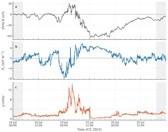
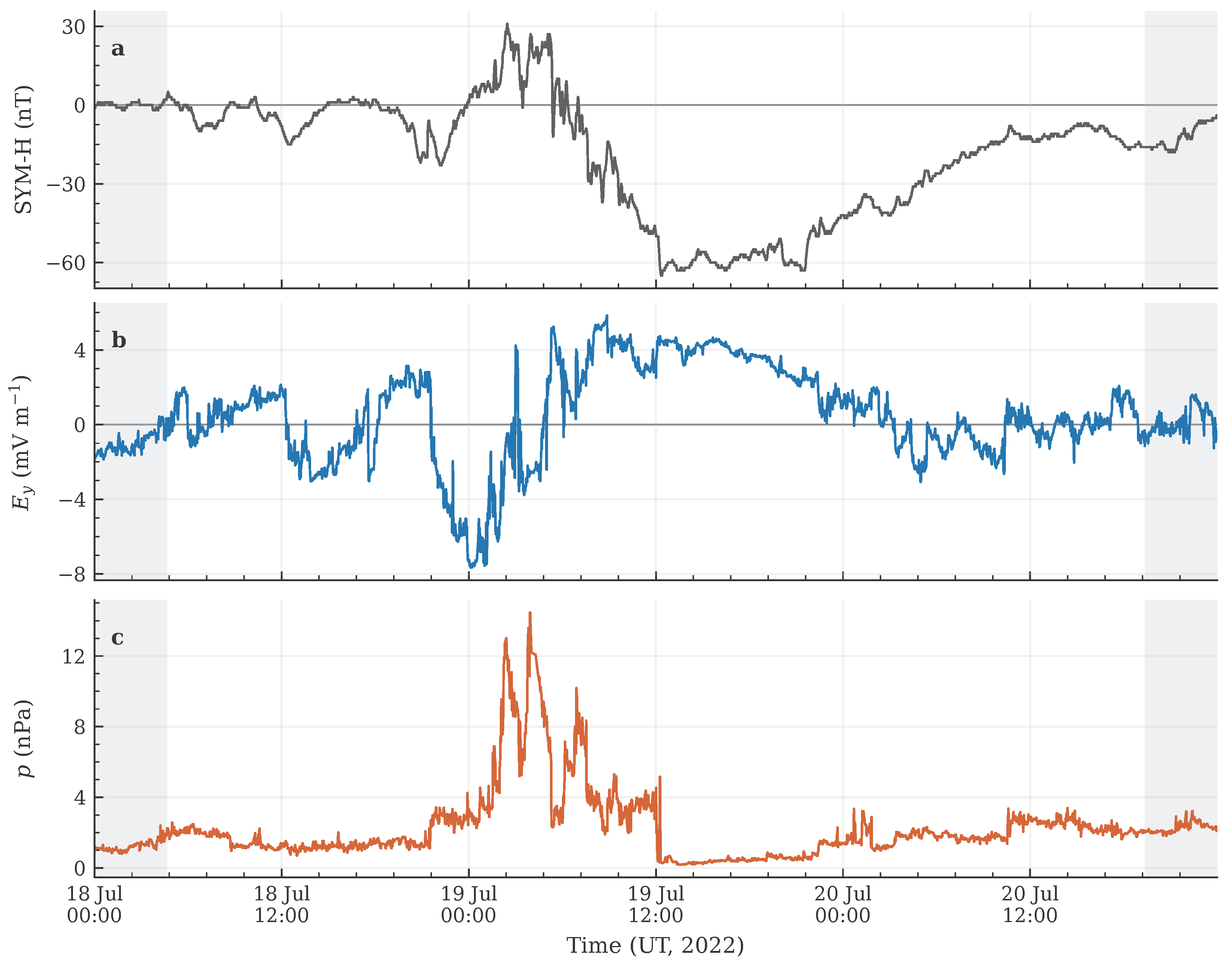
Figure 1 shows the three observed variables for Event 2, the 18–20 July 2022 interval. The plot provides temporal context; response timings are estimated from all eight intervals.

Figure 1. One-minute observations for Event 2 (18–20 July 2022), before filtering and standardization: (a) SYM-H (nT, dark grey), (b) dawn–dusk electric field $E_y$ (mV m⁻¹, blue), and (c) dynamic pressure p (nPa, orange). Grey shading marks the 279 min margins excluded from estimation. Solar wind series include interpolated samples (Supplementary Materials Section S1).

3. Methods

We represented the measured drivers, SYM-H, and their recent history through a state of preprocessed levels and temporal lags:

$${\mathbf{q}}_t={[{\tilde{E}}_{y,t},{\tilde{p}}_t,{\tilde{S}}_t]}^{\top },{\mathbf{Z}}_t={[{\mathbf{q}}_t^{\top },\dots ,{\mathbf{q}}_{t-m+1}^{\top }]}^{\top },m=5,D=3m=15.$$

(5)

The five blocks comprise the current sample and four preceding one-minute samples, defining the history explicitly represented in the state model. Tildes denote filtered and standardized levels, as specified below. We used a linear state model to relate spontaneous fluctuations to the response to an initial perturbation [15]:

$${\mathbf{Z}}_{t+1}=G{\mathbf{Z}}_t+{\mathit{\eta }}_{t+1}.$$

(6)

Here, $G\in {\mathbb{R}}^{D\times D}$ is a constant, spectrally stable companion matrix whose lower blocks shift the retained history. Innovations enter only the three current-level coordinates. The model assumes a centered stationary state with finite second moments and zero-mean additive innovations independent of preceding states and across time. An impulse changes one current coordinate while holding the other initial coordinates, including the retained history, fixed. The response per unit perturbation at lag k is the corresponding entry of $\mathcal{R}\left(k\right)=G^k$. Iterating Equation (6) and taking moments with ${\mathbf{Z}}_t$ gives, for a nonsingular $C_Z\left(0\right)$,

$$C_Z\left(k\right)=⟨{\mathbf{Z}}_{t+k}{\mathbf{Z}}_t^{\top }⟩=G^k{C}_Z\left(0\right),\mathcal{R}\left(k\right)=C_Z\left(k\right)C_Z{\left(0\right)}^{-1}.$$

(7)

This population identity follows from linear dynamics without requiring Gaussian distributions [15]. Its application to geomagnetic observations depends on the adequacy of the assumed state model; the covariance estimate and fitted propagator are compared below.

We used causal exponential high-pass filtering to subtract a slowly varying component from each level series. This filter uses only present and past samples. We prescribed ${\tau }_0=60$ min as an hourly reference for fast magnetospheric fluctuations, motivated by substorm development and directly driven injection. We chose ${\tau }_1=600$ min as a multihour reference for the slowly varying storm envelope, motivated by the evolution of solar wind forcing in interplanetary sheaths and ejecta. These prescribed scales define a common preprocessing convention across events. For Gaussian smoothing, the scale-separation argument of Baldovin et al. [20] balances contributions of orders ${\tau }_0/{\tau }_c$ and ${\tau }_c^2/{\tau }_1^2$ to the covariance approximation. Equating these orders with unit prefactors defines the reference scale

$${\tau }_c={\left({\tau }_0{\tau }_1^2\right)}^{1/3}={(60\times {600}^2)}^{1/3}\min \simeq 278.5\min .$$

(8)

We used this value as a common nominal reference for the Gaussian standard deviation and the exponential decay time. The kernels have distinct frequency responses: Gaussian symmetry cancels the first-derivative term when smoothing a slowly varying component, whereas the exponential kernel retains it. Thus, the scale derived from the Gaussian error balance serves as a prescribed reference for exponential filtering (Supplementary Materials Section S2). For an input $u_t$, its running average satisfies

$$s_t=(1-\alpha )s_{t-1}+\alpha u_t,\alpha =1-\exp (-\Delta t/{\tau }_c),\Delta t=1\min .$$

(9)

We initialized $s_1=u_1$ and used $u_t-s_t$ as the filtered series. We removed 279 samples from each end to retain the same timestamps in the primary analysis and sensitivity comparisons. Each retained level series was centered and divided by its standard deviation, calculated with the retained sample count as a divisor before constructing lagged blocks. Supplementary Materials Section S2 specifies the other preprocessing schemes and their boundary effects.

We estimated lagged covariances and fitted a regularized linear model separately for each event. For a retained record indexed by $t=1,\dots ,N_{\mathrm{ret}}$, let $N=N_{\mathrm{ret}}-m$ denote the number of states with one-step targets. The lagged covariance estimator is

$${\widehat{C}}_Z\left(k\right)={\displaystyle \frac{1}{N-k}}{\displaystyle \sum _{t=m}^{N_{\mathrm{ret}}-k-1}}{\mathbf{Z}}_{t+k}{\mathbf{Z}}_t^{\top }.$$

(10)

Each lag uses $N-k$ state pairs on the one-minute grid. Writing

$$X=[{\mathbf{Z}}_m,\dots ,{\mathbf{Z}}_{N_{\mathrm{ret}}-1}],Y=[{\mathbf{q}}_{m+1},\dots ,{\mathbf{q}}_{N_{\mathrm{ret}}}],$$

we fitted the companion predictive block on each complete trimmed event using ridge regularization with $\lambda ={10}^{-4}$:

$${\widehat{A}}_{\lambda }={\displaystyle \frac{Y{X}^{\top }}{N}}{\left[{\widehat{C}}_Z\left(0\right)+\lambda I_D\right]}^{-1},{\widehat{G}}_{\lambda }=\left(\begin{array}{cc}\multicolumn{2}{c}{{\widehat{A}}_{\lambda }}\\ I_{D-3}{0}_{(D-3)\times 3}\end{array}\right).$$

(11)

The top block predicts the next three levels; the lower block shifts the retained history by one sample.

We selected the perturbed driver and response observable using

$$B_{E_y}={\mathbf{e}}_1,B_p={\mathbf{e}}_2,L_S={\mathbf{e}}_3^{\top },L_{\Delta S}={\mathbf{e}}_3^{\top }-{\mathbf{e}}_6^{\top },$$

(12)

where ${\mathbf{e}}_j$ is the jth standard basis vector in ${\mathbb{R}}^D$. The difference selector extracts $\Delta {\tilde{S}}_{t+k}={\tilde{S}}_{t+k}-{\tilde{S}}_{t+k-1}$ at the response time. Because this increment is already a linear combination of retained levels, adding it as an independent state coordinate would introduce exact linear dependence. The increment uses the standard deviation of the SYM-H level, without separate rescaling; responses to standardized inputs are, therefore, dimensionless. Applying this selector at a fixed lag differs from differencing estimated level-response curves across lags, which use different sample pairs and normalizations. We calculated the covariance-based response and its fitted propagator counterpart as

$${\widehat{R}}_{\lambda }\left(k\right)=L{\widehat{C}}_Z\left(k\right){\left[{\widehat{C}}_Z\left(0\right)+\lambda I_D\right]}^{-1}B,R_{\mathrm{lin}}\left(k\right)=L{\widehat{G}}_{\lambda }^{k}B.$$

(13)

These driver–target channels use the full augmented covariance, conditioning on the other included coordinates. Finite-sample estimation and ridge regularization can produce differences between the covariance response and fitted propagator even when the population relation in Equation (7) holds. We assessed numerical conditioning and compared the covariance response with the fitted propagator over lags 1–15 min (Supplementary Materials Section S3). For the primary preprocessing, we extended this comparison to lags 16–40 and 41–120 min (Supplementary Materials Section S4).

We evaluated responses over $\mathcal{K}=\{0,\dots ,K_{\max }\}$, with $K_{\max }=40$ and physical lag $k\Delta t$. Let $r_e\left(k\right)$ denote ${\widehat{R}}_{\Delta S\leftarrow E_y,\lambda }\left(k\right)$ in event e. The eventwise peak lag, its median, and the peak of the equally weighted ensemble curve are

$$\begin{array}{cccc}\hfill {\tau }_e& =\Delta t \underset{k\in \mathcal{K}}{\mathrm{arg\; max}}\left|r_e\left(k\right)\right|,\hfill & \hfill {\tau }_{\mathrm{med}}& ={\mathrm{median}}_{e=1,\dots ,N_{\mathrm{ev}}}{\tau }_e,\hfill \end{array}$$

(14)

$$\begin{array}{cccc}\hfill \overline{r}\left(k\right)& ={\displaystyle \frac{1}{N_{\mathrm{ev}}}}{\displaystyle \sum _{e=1}^{N_{\mathrm{ev}}}}{r}_e\left(k\right),\hfill & \hfill {\tau }_{\mathrm{ens}}& =\Delta t \underset{k\in \mathcal{K}}{\mathrm{arg\; max}}\left|\overline{r}\left(k\right)\right|.\hfill \end{array}$$

(15)

Ties use the earliest lag, and the interquartile range (IQR) is the difference between linearly interpolated quartiles of ${\tau }_e$. The same definitions apply to the pressure increment-response channel. For the level response to $E_y$, we locate the negative minimum, ${\tau }_{S,e}=\Delta t {\mathrm{arg\; min}}_{k\in \mathcal{K}}{\widehat{R}}_{S\leftarrow E_y,\lambda }\left(k\right)$, to describe the largest downward response; we apply the same criterion to its ensemble mean. The IQR describes event dispersion; the peak of the mean curve also depends on response amplitudes and shapes. Primary peak estimates use the 0–40 min search window. As a sensitivity check, we extended the search to 0–120 min under exponential filtering, retaining the same records, preprocessing, state dimension, and ridge penalty (Supplementary Materials Section S4). For each extended lag, the covariance estimator retained its lag-dependent sample pairs and normalization. We report these timing statistics as descriptive summaries of the eight events.

For the plotted mean-response envelopes, we resampled eight event curves with replacement in 5000 replicates and calculated the 2.5th and 97.5th percentiles at each lag. These pointwise envelopes describe sensitivity to empirical event weights; they are neither simultaneous bands nor intervals for peak lags, and their population coverage is uncalibrated.

4. Results

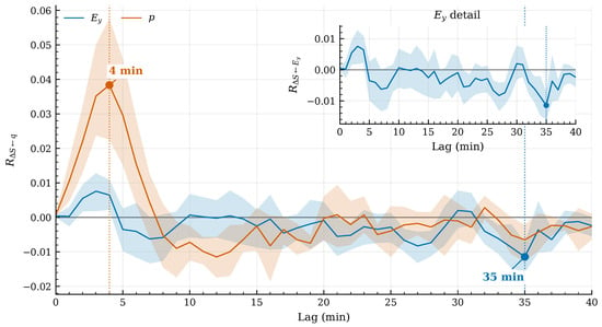
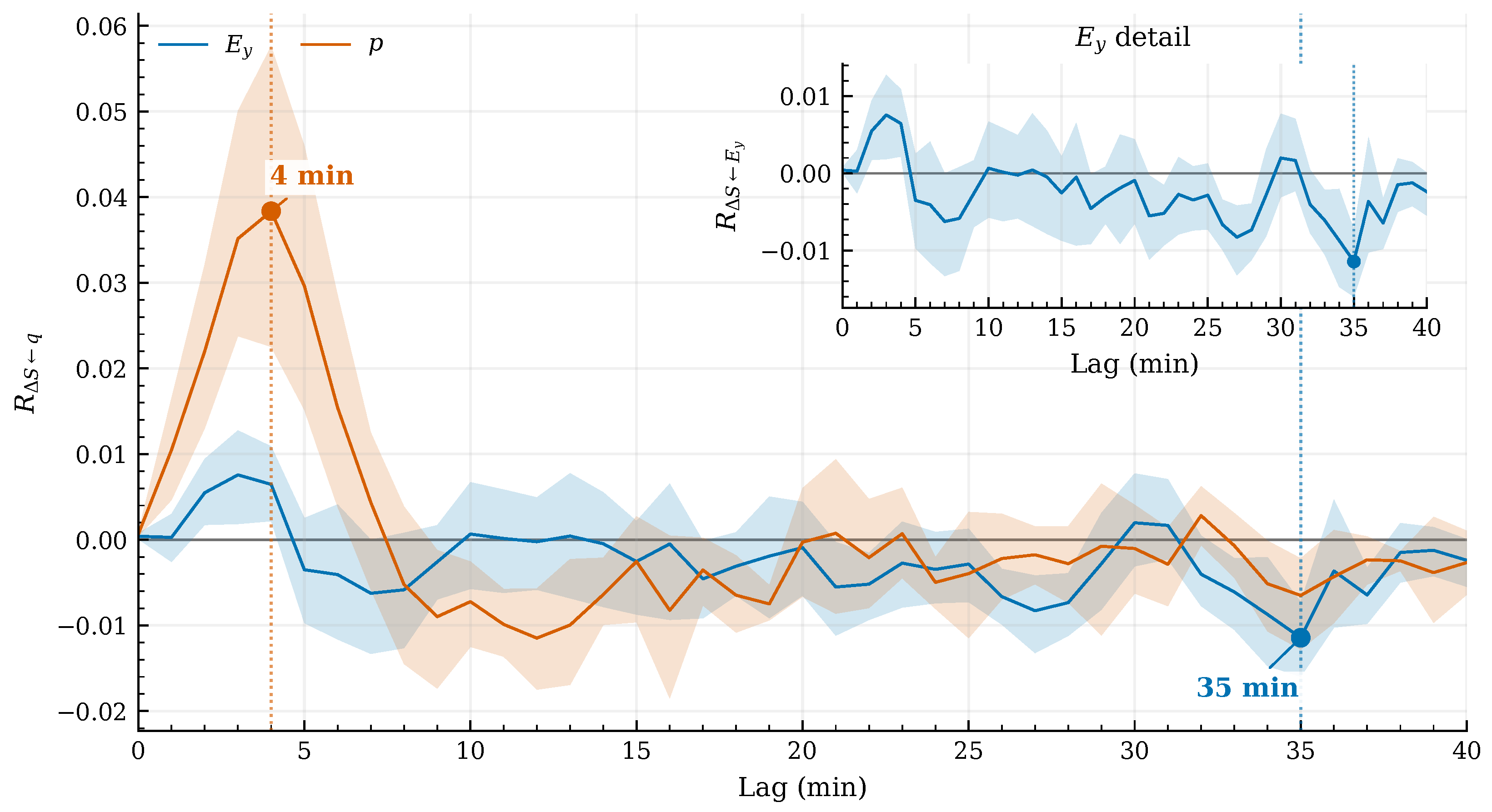
Under causal exponential filtering, pressure–response peaks in SYM-H increments occur earlier than electric-field-response peaks. Table 2 reports individual and aggregate peak lags; Figure 2 shows the ensemble-mean increment responses. The electric-field channel peaks between 5 and 35 min across events, with a median of 20 min and an IQR of 10.5 min. The mean curve reaches its largest absolute magnitude at 35 min. Pressure–response peaks range from 2 to 6 min, with a median of 4 min and an ensemble peak at 4 min.

Table 2. SYM-H response timing under causal exponential filtering, with S denoting the level and $\Delta S$ its one-minute increment. Peak searches cover 0–40 min. The increment columns give absolute-response peaks; the level column gives negative minima. Ensemble timings are extracted after averaging the eight curves. The dagger marks level-response minima at the 40 min upper boundary of the lag window.

Event	$\mathbf{\Delta }\mathit{S}\leftarrow {\mathit{E}}_{\mathit{y}}$ (min)	$\mathbf{\Delta }\mathit{S}\leftarrow \mathit{p}$ (min)	$\mathit{S}\leftarrow {\mathit{E}}_{\mathit{y}}$ (min)
1	35	6	39
2	21	4	36
3	5	4	40 †
4	21	3	39
5	7	4	35
6	34	2	38
7	19	4	40 †
8	16	3	38
Median	20	4	38.5
IQR	10.5	1	1.75
Peak of ensemble mean	35	4	40 †

Figure 2. Equally weighted mean SYM-H increment responses across the eight events in Table 1, using causal exponential filtering. Solid blue and orange curves denote the ensemble means for $E_y$ and p, respectively; the inset enlarges the electric-field response. Shaded bands are descriptive pointwise envelopes spanning the 2.5–97.5th percentiles of 5000 bootstrap replicates obtained by resampling the eight event curves with replacement. These envelopes are neither simultaneous confidence intervals nor uncertainties on peak lags. Dots and vertical dotted lines mark the largest absolute response magnitudes within 0–40 min, at 4 min for pressure and 35 min for electric field. Responses are dimensionless, with both driver and SYM-H levels standardized before calculating the increment response. In the ordinate label, q denotes the selected driver, $E_y$ or p.

Within the primary 0–40 min search window, the eventwise negative minima of the level response lie between 35 and 40 min, with a median of 38.5 min. The ensemble level-response minimum lies at the 40 min boundary, so this window does not resolve later minima. The 35 min increment-response ensemble peak is also close to this boundary.

The individual electric-field and pressure increment-response peak lags are unchanged under Gaussian filtering, linear detrending, and mean removal. The corresponding ensemble peaks remain at 35 and 4 min. Supplementary Materials Sections S2 and S3 report the preprocessing comparisons and dynamical diagnostics, respectively.

Extending the search to 0–120 min under exponential filtering changes the electric-field increment-response median from 20 to 41 min and its IQR from 10.5 to 48.5 min. The electric-field and pressure ensemble peaks remain at 35 and 4 min, and individual pressure peaks are unchanged. The ensemble level-response minimum shifts from the 40 min boundary to 102 min within the extended window (Supplementary Materials Section S4).

5. Discussion

The difference between eventwise and ensemble timing reflects how response curves contribute to their mean. Although events have equal weights, their standardized response amplitudes and shapes differ, so the mean curve need not peak at the median eventwise lag. The extended search changes the electric-field median while preserving the ensemble peak, showing that these summaries also differ in their sensitivity to the search horizon.

The early pressure response is consistent with rapid changes in magnetopause currents and the transmission of compressive disturbances through the magnetosphere [1]. For the 10 May 2024 event, the nearly 5 min delay reported in [21] runs from the shock detection at THEMIS-C in lunar orbit ($X\approx 49R_{\mathrm{E}}$) to the local onset of magnetic compression at GOES-16 ($X=6.29R_{\mathrm{E}}$), including upstream solar wind transit to the bow shock. OMNI instead provides observations shifted to the bow-shock nose [18,19], nominally at $X\approx 12–15R_{\mathrm{E}}$, where $R_{\mathrm{E}}$ is the Earth radius. From there, magnetosheath transit precedes the impact on the magnetopause, which launches an earthward fast magnetosonic disturbance, with an inferred propagation speed of $2800\mathrm{km}{\mathrm{s}}^{-1}$ in [21]. An illustrative timing budget allows 1–2 min for magnetosheath transit and a further 1–2 min for inward propagation and the development of geostationary and ground signatures, taking fast-mode speeds of order $1000–2800\mathrm{km}{\mathrm{s}}^{-1}$. These approximate contributions suggest a few-minute response; allowing for variations in geometry and plasma conditions gives an indicative 2–5 min timescale, consistent with our 4 min peak and eventwise range of 2–6 min. The comparison involves distinct observables: the local impulsive onset at GOES-16 in [21] and the peak estimated here. Our estimator locates the peak of the multivariate conditional impulse response of $\Delta \mathrm{SYM}-\mathrm{H}$ averaged over eight storms. Its timing is resolved on a one-minute grid and remains subject to uncertainties in OMNI time shifting [22]. The later electric-field response is compatible with convection and particle transport contributing to the development of the low-latitude disturbance [2,3,23]. These mechanisms can overlap: pressure-dependent injection models show that dynamic pressure can also modify ring-current development during strong storms [17]. Consequently, the two estimated channels describe conditional responses to measured drivers, while the SYM-H target retains the combined magnetic effects of several current systems. Their relative contributions require additional observables to resolve.

The relation between level and increment responses helps interpret the electric-field timing. In an injection–loss description, $dDs{t}^{\ast }/dt=Q-Ds{t}^{\ast }/\tau$, where $Ds{t}^{\ast }$ is the pressure-corrected index and $\tau$ is the ring-current decay time [2,3]. The injection term Q is negative when injection strengthens the negative disturbance, while the loss term drives $Ds{t}^{\ast }$ toward zero. An increment-response maximum characterizes the strongest change in the observed disturbance within the search window. The level response instead includes the accumulation of that change. Its ensemble minimum moves to a later lag in the extended search. These extrema characterize the selected observable within its search horizon; identifying maximum ring-current development requires a separate diagnostic. For a pressure correction $S^{\ast }=S-b\sqrt{p}+c$ with constant coefficients, backward differencing gives $\Delta S^{\ast }=\Delta S-b\Delta \sqrt{p}$ [2]. This identity applies to indices in physical units before preprocessing; separate standardization introduces observable-specific scaling. Conditioning on pressure retains uncorrected SYM-H as the target, with contributions from the superposed current systems.

Published response times place these results in a broader context, provided the indices and estimators are distinguished. For the lower-envelope auroral electrojet ($AL$) index, the prediction filters of Bargatze et al. [6] resolved responses near 20 and 60 min, interpreted in terms of direct driving and magnetotail energy release. Maggiolo et al. [7] reported peak correlation magnitudes at delays near 20 min for the polar-cap index, 35 min for the auroral electrojet ($AE$) index, and 80 min for SYM-H relative to IMF $B_z$. The polar-cap and AE correlations were negative, whereas the SYM-H correlation was positive. Using transfer entropy, Stumpo et al. [8] found a characteristic solar wind–SYM-H information-transfer delay near 60 min. Manshour et al. [16] also compared covariance-based responses with information-theoretic measures and found different characteristic delays. Our increment-response peaks fall within the range of rapid geomagnetic adjustments. The target variables, temporal conditioning, and estimators determine the physical interpretation of each quoted delay; assigning a common transport pathway requires independent evidence.

The unchanged individual increment-response peak lags across all four preprocessing schemes support a timing feature of this particular sample, while amplitudes and dynamical fits remain sensitive to preprocessing. We used the exponential filter in the primary presentation because its kernel respects temporal ordering. Gaussian filtering yields closer covariance–propagator agreement, a measure of model consistency whose relation to physical timing accuracy requires separate assessment. Scale-dependent coupling in the two storms studied by Alberti et al. [9] also cautions against identifying the selected filter scale with a universal magnetospheric timescale. Their fluctuation timescales and our response lags are distinct quantities. Here, ${\tau }_0$ and ${\tau }_1$ set a reproducible preprocessing convention whose applicability should be examined over additional events and activity regimes.

Under exponential filtering, the mean covariance–propagator discrepancy increases across the three lag ranges defined in Section 3, from 26.4% to 42.8% and 61.7% (Supplementary Materials Section S4). This full-matrix diagnostic combines finite-sample estimation, regularization, and possible departures from a stationary linear description; uncertainties in peak lags and individual driver–target channels require dedicated estimates. This increase with lag limits the dynamical interpretation of the estimated responses; channel-specific agreement near the 35 min peak remains to be assessed. Storm-phase variation is a relevant extension: the event-aligned information-transfer analysis of Stumpo et al. [10] found coupling localized in different phases of magnetic storms. Our whole-interval estimates average over such evolution. A larger event sample would allow phase-resolved comparisons without reducing each fit to very short records.

Peak selection can be sensitive to small amplitude differences. For Event 1, the electric-field increment response at 6 min reaches 99.92% of the absolute amplitude at the selected 35 min peak (Supplementary Materials Section S4). This near tie motivates eventwise peak-lag uncertainty estimates even when the selected peaks remain unchanged across preprocessing schemes.

Further checks should examine lag order, ridge strength, exponential-filter initialization, and input quality. The edge trim leaves a residual initialization contribution, and linear interpolation uses observations on both sides of data gaps; the present analysis is retrospective despite the one-sided filter. Plasma-input gaps affect 12.9–22.2% of samples across events, with gaps up to 25 min before trimming. Some gaps exceed the four-minute pressure ensemble lag, motivating sensitivity checks that account for both interpolation and filter memory. An expanded sample with documented selection and event-level uncertainty estimates would test whether the observed ordering persists beyond these eight intervals. Additional geomagnetic indices or in situ observations would help constrain the contributing current systems.

6. Conclusions

Using current and lagged levels of electric field, dynamic pressure, and SYM-H, we found earlier pressure–response peaks than electric-field-response peaks in SYM-H increments. This timing contrast persists across the four preprocessing schemes within the selected sample. Eventwise peak lags and the peak of the ensemble-mean curve provide complementary summaries: their difference shows why a single lag cannot describe both the individual events and their mean response.

The contrast is consistent with fast compressive and slower convective contributions to SYM-H, whose magnetic signature also reflects accumulated disturbance and losses. The electric-field median and level-response minimum depend on the search horizon, while the increment-response ensemble peaks persist under the tested extension. Increasing covariance–propagator discrepancies at longer lags and interpolated inputs limit the interpretation of these estimates as physical transport delays. Phase-resolved comparisons in a larger, documented sample, together with gap-aware and channel-specific validation, would assess how far the observed timing pattern extends beyond these eight intervals.

References

- Gonzalez, W.D.; Joselyn, J.A.; Kamide, Y.; Kroehl, H.W.; Rostoker, G.; Tsurutani, B.T.; Vasyliunas, V.M. What is a geomagnetic storm? J. Geophys. Res. Space Phys. 1994, 99, 5771–5792. [Google Scholar] [CrossRef] [Scilit]
- Burton, R.K.; McPherron, R.L.; Russell, C.T. An empirical relationship between interplanetary conditions and Dst. J. Geophys. Res. 1975, 80, 4204–4214. [Google Scholar] [CrossRef] [Scilit]
- O’Brien, T.P.; McPherron, R.L. An empirical phase space analysis of ring current dynamics: Solar wind control of injection and decay. J. Geophys. Res. Space Phys. 2000, 105, 7707–7719. [Google Scholar] [CrossRef] [Scilit]
- Iyemori, T. Storm-time magnetospheric currents inferred from mid-latitude geomagnetic field variations. J. Geomagn. Geoelectr. 1990, 42, 1249–1265. [Google Scholar] [CrossRef] [Scilit]
- Wanliss, J.A.; Showalter, K.M. High-resolution global storm index: Dst versus SYM-H. J. Geophys. Res. Space Phys. 2006, 111, A02202. [Google Scholar] [CrossRef] [Scilit]
- Bargatze, L.F.; Baker, D.N.; McPherron, R.L.; Hones, E.W., Jr. Magnetospheric impulse response for many levels of geomagnetic activity. J. Geophys. Res. Space Phys. 1985, 90, 6387–6394. [Google Scholar] [CrossRef] [Scilit]
- Maggiolo, R.; Hamrin, M.; De Keyser, J.; Pitkänen, T.; Cessateur, G.; Gunell, H.; Maes, L. The Delayed Time Response of Geomagnetic Activity to the Solar Wind. J. Geophys. Res. Space Phys. 2017, 122, 11,109–11,127. [Google Scholar] [CrossRef] [Scilit]
- Stumpo, M.; Consolini, G.; Alberti, T.; Quattrociocchi, V. Measuring Information Coupling between the Solar Wind and the Magnetosphere–Ionosphere System. Entropy 2020, 22, 276. [Google Scholar] [CrossRef] [Scilit]
- Alberti, T.; Consolini, G.; Lepreti, F.; Laurenza, M.; Vecchio, A.; Carbone, V. Timescale separation in the solar wind–magnetosphere coupling during St. Patrick’s Day storms in 2013 and 2015. J. Geophys. Res. Space Phys. 2017, 122, 4266–4283. [Google Scholar] [CrossRef] [Scilit]
- Stumpo, M.; Benella, S.; Consolini, G.; Alberti, T. Dynamical information flow within the magnetosphere-ionosphere system during magnetic storms. Rend. Lincei. Sci. Fis. E Nat. 2023, 34, 1–9. [Google Scholar] [CrossRef] [Scilit]
- Granger, C.W.J. Investigating Causal Relations by Econometric Models and Cross-spectral Methods. Econometrica 1969, 37, 424–438. [Google Scholar] [CrossRef] [Scilit]
- Schreiber, T. Measuring Information Transfer. Phys. Rev. Lett. 2000, 85, 461–464. [Google Scholar] [CrossRef] [Scilit] [PubMed]
- Runge, J.; Bathiany, S.; Bollt, E.; Camps-Valls, G.; Coumou, D.; Deyle, E.; Glymour, C.; Kretschmer, M.; Mahecha, M.D.; Muñoz-Marí, J.; et al. Inferring causation from time series in Earth system sciences. Nat. Commun. 2019, 10, 2553. [Google Scholar] [CrossRef] [Scilit] [PubMed]
- Marconi, U.M.B.; Puglisi, A.; Rondoni, L.; Vulpiani, A. Fluctuation–dissipation: Response theory in statistical physics. Phys. Rep. 2008, 461, 111–195. [Google Scholar] [CrossRef] [Scilit]
- Baldovin, M.; Cecconi, F.; Vulpiani, A. Understanding causation via correlations and linear response theory. Phys. Rev. Res. 2020, 2, 043436. [Google Scholar] [CrossRef] [Scilit]
- Manshour, P.; Balasis, G.; Consolini, G.; Papadimitriou, C.; Paluš, M. Causality and Information Transfer Between the Solar Wind and the Magnetosphere–Ionosphere System. Entropy 2021, 23, 390. [Google Scholar] [CrossRef] [Scilit]
- Xie, H.; Gopalswamy, N.; St. Cyr, O.C.; Yashiro, S. Effects of solar wind dynamic pressure and preconditioning on large geomagnetic storms. Geophys. Res. Lett. 2008, 35, L06S08. [Google Scholar] [CrossRef] [Scilit]
- King, J.H.; Papitashvili, N.E. Solar wind spatial scales in and comparisons of hourly Wind and ACE plasma and magnetic field data. J. Geophys. Res. Space Phys. 2005, 110, A02104. [Google Scholar] [CrossRef] [Scilit]
- King, J.; Papitashvili, N. One Min and 5-Min Solar Wind Data Sets at the Earth’s Bow Shock Nose. Available online: https://omniweb.gsfc.nasa.gov/html/HROdocum.html (accessed on 29 September 2026).
- Baldovin, M.; Cecconi, F.; Provenzale, A.; Vulpiani, A. Extracting causation from millennial-scale climate fluctuations in the last 800 kyr. Sci. Rep. 2022, 12, 15320. [Google Scholar] [CrossRef] [Scilit]
- Li, S.; Pi, G.; Němeček, Z.; Šafránková, J.; Leonard, T.W.; Sun, Y.Y. Evolution of Magnetospheric Boundary Layers Under the 10 May 2024 ICME Impact. Geophys. Res. Lett. 2026, 53, e2025GL121067. [Google Scholar] [CrossRef] [Scilit]
- Di Matteo, S.; Sivadas, N. Solar-wind/magnetosphere coupling: Understand uncertainties in upstream conditions. Front. Astron. Space Sci. 2022, 9, 1060072. [Google Scholar] [CrossRef] [Scilit]
- Daglis, I.A.; Thorne, R.M.; Baumjohann, W.; Orsini, S. The terrestrial ring current: Origin, formation, and decay. Rev. Geophys. 1999, 37, 407–438. [Google Scholar] [CrossRef] [Scilit]
Disclaimer/Publisher’s Note: The statements, opinions and data contained in all publications are solely those of the individual author(s) and contributor(s) and not of MDPI and/or the editor(s). MDPI and/or the editor(s) disclaim responsibility for any injury to people or property resulting from any ideas, methods, instructions or products referred to in the content. |
© 2026 by the authors. Licensee MDPI, Basel, Switzerland. This article is an open access article distributed under the terms and conditions of the Creative Commons Attribution (CC BY) license.