Abstract
The Internet of Things (IoT) is an exponentially growing emerging technology, which is implemented in the digitization of Electronic Health Records (EHR). The application of IoT is used to collect the patient’s data and the data holders and then to publish these data. However, the data collected through the IoT-based devices are vulnerable to information leakage and are a potential privacy threat. Therefore, there is a need to implement privacy protection methods to prevent individual record identification in EHR. Significant research contributions exist e.g., p+-sensitive k-anonymity and balanced p+-sensitive k-anonymity for implementing privacy protection in EHR. However, these models have certain privacy vulnerabilities, which are identified in this paper with two new types of attack: the sensitive variance attack and categorical similarity attack. A mitigation solution, the -sensitive k-anonymity privacy model, is proposed to prevent the mentioned attacks. The proposed model works effectively for all k-anonymous size groups and can prevent sensitive variance, categorical similarity, and homogeneity attacks by creating more diverse k-anonymous groups. Furthermore, we formally modeled and analyzed the base and the proposed privacy models to show the invalidation of the base and applicability of the proposed work. Experiments show that our proposed model outperforms the others in terms of privacy security (14.64%).
1. Introduction
The current highly-connected technological society generates a huge amount of digital data—termed Big Data, collected through internet-enabled devices, termed the Internet of Things (IoT) [1]. Billions of these IoT devices sense and collect the data e.g., the patient’s Electronic Health Records (EHR) [1,2,3,4]. The collected data are then shared with corporate or government bodies for research and policymaking. However, the privacy of the individual records is an important goal when sharing data that is collected through the IoT enabled devices [1,2,3,4,5,6]. This is because these data contain names or some unique identification (explicit identifiers—), such as age, gender, zip code (quasi-identifiers—), and some health-related private information (sensitive attributes—) [7,8,9,10,11,12]. To preserve privacy, eliminating the before sharing or publishing the data is not enough [11]. For an attacker or an adversary, the quasi-identifiers (QIs) are the partial identifiers that can be used to link to some externally available data e.g., voting or census data, to identify an individual , known as a linking attack [10,11,12].
To implement data privacy, a lot of cryptographic techniques [13,14] have been proposed. However, these techniques have high computational overheads. Another simple approach is data anonymization. Data anonymization is about concealing an individual’s identity in a small crowd of records before data publishing. The publishing of such anonymized records are known as Privacy Preserving Data Publishing (PPDP) [11]. A plethora of PPDP methods have been proposed [7,8,9,10,11,12,15,16,17,18,19]. These techniques are broadly classified into:
- Identity disclosure prevention: Generalizing [7,8,9] the QI values of a group of records from more specific values to less specific values e.g., k-anonymity [7,8], where every record should be indistinguishable from at least k-1 other records. An individual having probability higher than 1/k cannot be re-identified by an intruder/attacker.
- Attribute disclosure prevention: Preventing to reveal private information ( information) about an individual. Examples are l-diversity [15] and t-closeness [16] privacy models.
In this paper, a variance-based privacy model is proposed to prevent attribute disclosure risk. For sensitive attribute privacy, the p+-sensitive k-anonymity, (p, α)-sensitive k-anonymity [17] privacy model is a state-of-the-art privacy model where the sensitive values are categorized into four categories. For creating a k-anonymous group of records called an equivalence class (EC), a l-diversity [15] is applied. However, two new possible attacks are applied: sensitive variance attack and categorical similarity attack. These attacks breach the privacy of the p+-sensitive k-anonymity and (p, α)-sensitive k-anonymity [17] algorithm, due to the values from the single sensitive category or a low diversity at category level. The proposed mitigation solution: the -Sensitive k-anonymity privacy model, is a numerical measure of privacy strength for thwarting the attribute disclosure risk. The proposed approach also appends small amounts of noise tuple(s) to increase the variability in an EC, if needed. To minimize the utility loss, the proposed algorithm uses a bottom-up generalization (i.e., the local recoding mechanism [18]) because it minimally distorts the data compared to global recoding techniques [12]. The following section presents the motivation of our work.
1.1. Motivation
Broadly examining the PPDP models for preventing attribute disclosure risk [11,15,16,17,18], it was concluded that the worthiness of each model exists in the diversity of an EC where the sensitive values belongs to different categories. Such variability of values creates a diverse EC. Different privacy models employ different techniques to achieve variability in k-anonymous ECs. The repeated frequencies of same sensitive values are the only obstruct in achieving the required diversity in an EC. The privacy models in [17] and [18] provide a meaningful approach in dealing with the attribute disclosure problem, however the following limitations have been observed.
- p+-sensitive k-anonymity and (p, α)-sensitive k-anonymity [17]: This model is a modified version of the p-sensitive k-anonymity [19], for preventing a similarity attack. However, the p+-sensitive k-anonymity and (p, α)-sensitive k-anonymity models have zero diversity at the category level, which may lead to a categorical similarity attack. A more powerful possible attack by an adversary is the sensitive variance attack, due to the low variability at category level. With an upsurge in the adversary’s knowledge (background knowledge—BK) the privacy level can be breached, which may cause attribute disclosures. The proposed -sensitive k-anonymity privacy model provides a privacy solution to prevent all such attacks.
- Balanced p+-sensitive k-anonymity and (p, α)-sensitive k-anonymity [18]: This model is an enhanced version of p+-sensitive k-anonymity model. It balances the categorical level sensitive attributes in each EC. However, it still has low diversity at category level and works only for more than three k-anonymous size ECs.
To solve the problems of homogeneity, categorical similarity, and sensitive variance attacks in the p+-sensitive k-anonymity and (p, α)-sensitive k-anonymity model [17], we propose the -Sensitive k-anonymity privacy model in this paper. The categorical level similarity and small EC size problems in the balanced p+-sensitive k-anonymity and (p, α)-sensitive k-anonymity model [18] are also addressed by achieving a more balanced and diverse EC even at the category level and its execution on small k size EC, i.e., k = 2.
1.2. Contributions
The proposed -sensitive k-anonymity privacy model multiplies variance () of a fully diverse EC with an observed value (observation 1) which produces a threshold value . The value ensures prevention against attribute disclosure in an EC which collectively results in the privacy of the given dataset.
The contributions of this paper are as follows:
- A new -sensitive k-anonymity privacy model is proposed where privacy in an EC is achieved through a threshold value, i.e., . The value for an EC is obtained by multiplying variance and an observation value. The variance-based diversity in an EC prevents the sensitive variance attack, which automatically prevents the categorical similarity attack. In the proposed model, the values checking is not only performed with next ECs, but a cross check is also performed during the last EC. If the required privacy is not achievable with the existing values, then a noise is added for the required diversity.
- We formally modeled and analyzed the base model in [17] and the proposed -sensitive k-anonymity privacy model using High Level Petri-Nets (HLPN).
- Based on the above points, simulation results show that our proposed -sensitive k-anonymity model has only 0.002679% higher privacy leakage than its counterpart p+-sensitive k-anonymity model which has 14.65% higher privacy leakage with the base line privacy.
Paper Organization. The remainder of the paper is organized as follows. Section 2 explains related work. Preliminaries are discussed in Section 3. The considered attacks and problem statement in p+-sensitive k-anonymity along with its formal analysis are presented in Section 4. Section 5 discusses the proposed -sensitive k-anonymity model and its formal analysis. In Section 6, the experiments and evaluations are provided. Section 7 concludes the paper.
2. Related Work
In this section, the literature related to the proposed privacy model is studied from various aspects. The data collected through the various IoT enabled devices [1,2,3,4,5,6,20,21] must be anonymized before publishing because of the private information contained in it. Anonymized data are published for the sake of its maximum utility without disclosing the private information of an individual. For anonymization, the privacy models can be broadly classified into semantic [22,23] or syntactic [7,8,9,10,11,12,13,14,15,16,17,18,19] approaches. The semantic privacy models add a random amount of noise for preserving privacy, e.g., differential privacy models [22,23]. In differential privacy, the deletion or addition of an individual’s record or noise does not affect the data analysis results while preserving the privacy. Syntactic privacy models create a k-indistinguishable [7] ECs. In syntactic privacy, two main privacy disclosure risks are: identity disclosure [7,8,9,10,12] and attribute disclosure [11,15,16,17,18]. The k-anonymity [7,8] is an example of preventing identity disclosure that generalizes a set of records with respect to QIs. These k-anonymous records are indistinguishable from other k-1 records in a dataset. However, k-anonymity lacks the ability to provide attribute level protection. Attribute disclosure releases the value of confidential attributes corresponding to an identified individual record. Although in l-diversity [15], l distinct groups for the in an EC are required. However, the skewness and similarity attacks can breach the privacy because l-well sensitive attribute groups are not always possible over the existing s. Similarly for t-closeness [16], the threshold for and its distance distribution in an EC has low data utility, and the earth mover distance (EMD) is not an efficient prevention for attribute linkage [24,25].
In [26] by Torra, identity and attribute disclosure were both addressed. Jose et al. [27] proposed an adaptive two-step iterative anonymization approach. A privacy leakage for an attribute linkage attack was possible because of having numerous versions. An extended k-anonymity model was proposed by Rahimi et al. [28] to protect identity and attribute information. However, a BK attack is possible because the publisher is unaware of the adversary’s knowledge. The k-join-anonymity model proposed by Sowmiyaa et al. [29] was the same as k-anonymity, which focuses only on identity disclosure risk. The (α, k)-anonymity model proposed by Wong et al. [30], used a global recoding technique, which has a high utility loss and, due to table linkage attack, it was susceptible to the disclosure of attributes.
The (k, e)-anonymization model proposed by Zhang et al. [31] publishes separate tables, consisting of and QI to reduce the relationship between them, and where instead of generalization, a permutation-based approach has been adopted. Although in aggregated search, not using QI-generalization is recommended for accuracy improvement. However, a probabilistic attack is possible over the due to the one-time publication of the microdata. The (ɛ, m)-anonymity model [32] deals with the numeric , however it is limited to work for categorical . Xiao et al. [33] worked on personalized anonymity that uses a greedy personalized generalization approach. This model de-associated and QI instead of modifying the association between them.
In Reference [19], the p-sensitive k-anonymity found the closest neighbor. This model was then improved by Sun at al. [17] with a top-down specialization. The generated anonymized datasets should be from at least p distinct values categories for each EC. However, the developed algorithm in [17] is vulnerable to privacy leakage from sensitive variance, categorical similarity, and homogeneity attacks. In this paper, these privacy limitations were mitigated using the proposed –sensitive k-anonymity algorithm. The proposed privacy model is a syntactic privacy model for preventing attribute disclosure risk, which adds a fixed amount of noise to create k-anonymous ECs.
3. Preliminaries
Let an original Microdata Table (MT (i.e., Table 1a) be the private static data (i.e., one-time release) for a publisher to publish. The is a tuple that belongs to an individual i, such that EI = {, }, QI = {, }, and S = {} (this work considers only single ). The k-anonymized data essentially consists of and , while are removed. This is because an adversary can link the with some external information (e.g., voter or census data) to perform a record linkage attack (i.e., identity disclosure) [34]. However, the k-anonymous values prevent the record against the record linkage attack in an EC. For example, consider some common diseases in a 2-anonymous (Table 1b) obtained from the original microdata Table 1a. Table 2 summarizes the notations used in this paper.

Table 2.
Summary of notations used.
Definition 1.
k-anonymity [7,8]: Relation R having over the schema R(A1,A2, …, An) in a masked microdata table T’ is said to be k-anonymous if and only if, for any combination t() values from start to end, is greater than or equal to k in R.
where k is the anonymity level (as shown in Table 1b). The k-anonymity model blends the k records into at least a k-1 crowd but it does not impose any restrictions on the algorithm to sufficiently protect the individuals. Consequently, the probability of linking a victim to a specific record through s is at most 1/k.
Definition 2.
l-Diversity [15]: A QI block in a masked microdata table T’ having m QI-blocks is l-diverse, if it contains more than or equal to l well significant values. In an l-diverse modified microdata table T’, every QI block is l-diverse.
Definition 3.
t-closeness [16]: An EC is considered as t-closed if the distance between the distribution of the sensitive data in a class and the distribution of sensitive data in the whole table is equal to or less than threshold t. If every EC is t-closed, the whole table is t-closed. To calculate the distance while studying the transportation problem, researchers have explored some methods [33,35]. However, most of them focused on the Earth Mover Distance (EMD) method [15,36]. The EMD(P, Q) measures the minimum cost for transforming one distribution P to another distribution Q. It depends on the amount and distance of mass moved.
Definition 4.
p-sensitive k-anonymity [19]: The masked microdata table T’ is p-sensitive k-anonymous if it is k-anonymous and each EC in T’ has at least p distinct values.
where G represents an EC that already satisfies k-anonymity and is a set of and . The value of must be equal to or greater than p, where represents distinct values in an EC.
Definition 5.
Categorical similarity attack: If an adversary knows that the l-diverse modified microdata T’ (satisfying k-anonymity and l-diversity) has sensitive values belong to the single sensitive category in an EC from a p distinct categories.
Definition 6.
Sensitive variance attack: The privacy leakage in an EC due to the low variability of sensitive values from p distinct categories.
Definition 7.
High-Level Petri Nets (HLPN) [37]: The behavior of the system with its mathematical properties are modeled specifically via HLPN. An HLPN is a combination of 7-tuples where represented by circles are the set of places. is the set of transitions in the system represented by rectangular boxes, such that . represents the flow relations such that . . maps places to the data types. represents the rules or properties for transitions that verify the correctness of the underlying system. represents labels on , and is the initial marking.
The following section reviews the p+-sensitive k-anonymity model, to highlight its shortcomings concerning sensitive variance or an S-Variance attack.
4. Problem Statement
Definitions 8 and 9 describe the p+-sensitive k-anonymity and -sensitive k-anonymity models [17], respectively.
Definition 8.
p+-sensitive k-anonymity [17]: A masked microdata T’, fulfills k-anonymity and for each value belongs to distinct categories must be equal to or greater than p for each EC in T’.
where C depicts values categorizations that already fulfill a p-sensitive k-anonymous approach. represents distinct categories in Table 3 [17] and must be equal to or greater than p. Table 4a obtained from Table 1a, shows p+-sensitive k-anonymity model in which p = 2, k = 4 and c = 2. The ECs column in Table 4a is not part of a published table.
Table 3.
Category table.
Definition 9.
-sensitive k-anonymity [17]: A modified microdata table T’ that fulfills the k-anonymity property and there must be p distinct sensitive attribute values in each QI-group having a minimum weight of at least .
where represents all groups in masked micro table T’ that already fulfill the p-sensitive k-anonymity property. Weight should be assigned to each category and each sensitive value p must have weight in each category i.e., that must be at least . Table 4b obtained from Table 1a, shows -sensitive k-anonymity.
The sensitive variance and categorical similarity attacks have minor difference concerning the variability of in an EC. The sensitive variance attack is more powerful than categorical similarity attack, i.e., categorical similarity attack sensitive variance attack. Therefore, the attribute disclosure through the sensitive variance attack automatically covers the disclosures through the categorical similarity attack. The EC2 and EC3 in Table 4a obtained through the p+-sensitive k-anonymous approach have categorical similarity and sensitive variance attacks and are explained in Table 5. Table 5 shows the variance calculation for these ECs, where a high variance for more diverse EC2 and small variance for less diverse EC3 can be seen.
Table 5.
Variance calculation for different equivalence classes (ECs) in Table 4a.
To calculate the variance of the ECs, an ordered weight is given to the values in such a way that the higher the frequency (f), the lower the weight (x) will be. For example, consider EC3 in Table 4a, i.e., Flu = 2, Cancer = 1, HIV = 1. The numeric value against each sensitive value represents its frequency occurrence in EC3. If an EC, e.g., EC2 is fully diverse i.e., size 4 and 4-diverse, then the order weight will be Hepatitis = 1, Phthisis = 1, Asthma = 1, Obesity = 1. In EC2, because of having a single occurrence for each value, has a higher variance than EC3.
An adversary, using the category table (Table 3), can analyse the ECs in Table 4a and Table 4b published in [17]. The variability in some of the ECs is low concerning the category table. Therefore, the adversary can isolate the sensitive values that belong to a specific category and hence to individual records, and thus breaches the identity of an individual.
Critical Review of p+-Sensitive k-Anonymity Model
We formally modeled the p+-sensitive k-anonymity algorithm to check its invalidation concerning a sensitive variance attack. The detail formal verification of the working of p+-sensitive k-anonymity privacy model along with its properties is given in [18] from Rule 1 to Rule 7, which gets original data input from the end-user and processes it. The sensitive variance attack over the p+-sensitive k-anonymity model is shown in Figure 1, where the arrow heads show the data flow. Table 6 shows variable types and their descriptions. The places and its description are shown in Table 7. The attacker model in Figure 1 consists of three entities: the end-user, the adversary, and the trusted data publisher.
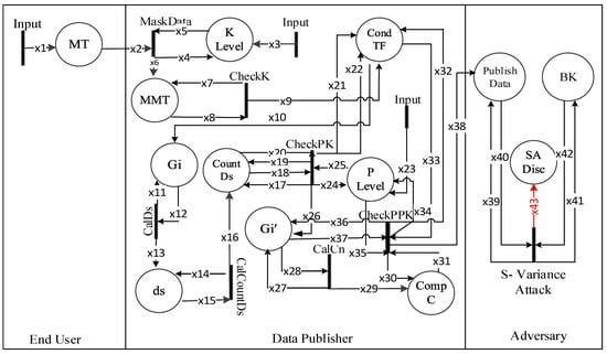
Figure 1.
HLPN for p+-sensitive k-anonymity attack model.
Table 6.
Types used in high-level Petri nets (HLPN) for p+-sensitive k-anonymity.
Table 7.
Data-types, places, and their mapping.
In Figure 1, Transitions , which are input to the HLPN model, consist of patients’ records (original data). A trusted data publisher further processes the data to minimize an attribute disclosure risk. Generalization and removing identifying attributes transform the data into masked data. After generalization, the masked microdata table is ready to be published. An adversary then exploits the published data for its benefits.
In this paper, the first seven rules in [18] are outlined briefly. For input k, the data publisher processes the original data to perform data generalization via the function and each EC is stored at place the micro mask table (MMT); The publisher confirms the k-anonymity condition. If successful, variable is set to . For each EC, the function calculates the distinct values and stores its count at place . To further process the array of t , the function counts the and stores it at place . Before the calculation of , p-sensitive k-anonymity is verified in masked data. Transition checks at least p distinct values in each EC in the whole table. stores the input transition p value for comparison. Apart from the checking condition for k-anonymity, another checking for p value is done. If it returns it means the data already fulfills k-anonymity. This concludes a successful transition, ensures the p-sensitive k-anonymous property. Next, computing values categories using function . Both values and categories are stored at place for further processing. Actual improvement to the prior model and source for p+-sensitive k-anonymity is the transition . Distinct categories are calculated in a column, using the sensitive values. stores this ‘number’ of distinct categories. The involved in each EC is checked with transition to confirm that there must be at least p distinct categories. The minimum value for p is 2. The p+-sensitive k-anonymity properties are fulfilled if the variable returns .
The p+-sensitive k-anonymity model is highly vulnerable against a sensitive variance attack. The main reason is the existence of non-diverse (low variance) values similar to ‘Flu’ in Table 4a and Table 4b, and ‘HIV’ in Table 4b. In Rule (1) through function -, an adversary performs an attack on the released data using some external source of information, i.e., BK. In Rule (1):
The adversary takes the union of the published data with the external information and BK to plot an EC. In this way, specific individuals correspond to some specific ECs that belong to homogenous categories and hence sensitive values from a specific category disclose an individual. Therefore, a sensitive variance attack occurs due to low variance in corresponding ECs.
5. The Proposed -Sensitive k-Anonymity Privacy Model
5.1. Threshold -Sensitivity
The goal of the proposed -Sensitive k-anonymity privacy model is to prevent the attribute disclosure of the individual records in MT, collected through the IoT [2,3,4,5,6] enabled devices. Each EC in MT must satisfy the threshold value. The -Sensitivity, is the product of variance () and Observation 1 (µ) as shown in Equation (1).
The variance value represents the diversity in an EC. High variance means high diversity in an EC and vice versa, since achieving 100% diversity is almost impossible in all cases. However, the variance-based optimal frequency distribution of values with some fixed amount of noise addition achieves an enhanced data privacy in an EC. The proposed method in this paper is simple and effective. During examining each EC, if the variance of an EC is greater than i.e., fully diverse, the next EC is examined. Otherwise, the variance for the same EC is increased by swapping the values from the successor ECs or by adding some noise records, to make it above . Because of the required noise addition, our proposed model implies -differential privacy [22,23] but the proposed approach is a syntactic anonymization [9] approach.
5.1.1. Variance ()
The variance calculation in Table 5 for ECs depicts the variability in a numerical form. To standardize the value for different size ECs, to prevent the sensitive variance attack, initially, we consider a fully diverse EC, e.g., if EC size = 2 variance = 0.25, if EC size = 3 variance = 0.67, if EC size = 4 variance = 1.25, if EC size = 5 variance = 2, and so on, then multiplying the variance with an observed value from Observation 1 ().
5.1.2. Observation 1 ()
A decimal multiplied part: Observation 1 (µ), for getting , the threshold value has full control over the EC diversity. During the simulation in Python, different values for µ were checked to get a suitable value. After executing the dataset for different k size ECs, the values of µ in the range of 0.5 to 0.9 were concluded. A smaller observed µ value results in the frequent repetition of sensitive values in an EC, and higher observed value produces a more diverse EC. However, “what observed value should be chosen for different size ECs?”, is explained below.
Consider again, the 2+-Sensitive 4-anonymous Table 4a, EC2 variance = 1.25, and EC3 variance = 0.69. The difference is because of the duplicated sensitive value i.e., Flu, in EC3. We propose an efficient way of removing the frequency repetition of sensitive values to achieve a more diverse EC. For this, we calculated the value. For example, consider a fully diverse EC of size 4 with variance = 1.25 and multiply it with an observed value, ranges between 0.5 and 0.9. Since, 1.25 * 0.5 = 0.625 is less than 0.69 and 1.25 * 0.6 = 0.75, which is greater than 0.69. The difference between the two values i.e., 1.25 and 0.69, is because of only one duplicated value “Flu”. Thus, it depends on privacy requirements and the level of diversity we are interested to achieve. In this paper, we perform a very strict calculation to get fully diverse ECs. Therefore, for example in the implementation part of the proposed Algorithm 1, we multiply a variance of 4 size EC with an observed value µ= 0.6 to have a fully diverse EC. The same technique is applied to all other ECs as well. The obtained in this way in line 8 of the proposed Algorithm 1 in Section 5.2, is then checked in the conditional part at line 10 inside a loop to check all ECs concerning requirements.
Definition 10.
-Sensitive k-anonymity: The modified microdata table T’ fulfills -sensitive k-anonymity, if it fulfills k-anonymity and for each EC in T’, the variance for each EC must be at least .
where G represents a QI-group or EC that already satisfies k-anonymity and is a set of and . The value of must be equal to or greater than p, where is the number of distinct sensitive values in a QI-group. The proposed -sensitive k-anonymity model produces the anonymized Table 8a (with noise) from the original microdata Table 1a and Table 8b (without noise) from Table 4b. The values in Table 8a and Table 8b are generalized through local recoding (bottom-up generalization) which improves the utility of the anonymized data. The 4-diverse ECs in Table 8a and Table 8b have sensitive values from a minimum of three different sensitive categories in Table 3. Therefore, these tables have more attribute privacy and are more protected from a sensitive variance attack.
5.2. The Proposed -Sensitive k-Anonymity Algorithm
The proposed -sensitive k-anonymity algorithm starts execution by checking the k size to create an EC (minimum cardinality k = 2), at line 3. The algorithm can be executed on different size of k. However, if the minimum cardinality fails, the condition becomes and jumps to line 50. If it is , the loop works from line 5 to 7, to calculate the variance for each m size or that belongs to k-anonymous ECs and assigns them to an array i.e., .
Line 8 multiplies an average observed value and variance for an EC to get a threshold (i.e., Equation (1)). This value ensures the maximum level of diversity in an EC. mainly depends on . If is smaller for an EC, low diverse EC will be obtained and vice versa. What level of diversity we want to have in an EC is completely controlled by . Deeply observing l-diversity [15] and t-closeness [16] and performing experiments while executing the algorithm in Python, the value is kept to achieve maximum diversity. The algorithm starts working from lines 9–49, which checks the obtained variances against user input k for each m size EC to . At line 10, if is greater than , line 46 is executed and the algorithm moves on to next EC. If it is less than , the current EC is named as , and the next index EC is named as . Lines 12–45, each part inside if statement has two major functionalities; swapping and require noise addition.
The else part of an if statement executes the ECs from first till , and its first part processes the last EC (lines 13–25). At line 12, if is the last class, i.e., , then from the value of is calculated. Similarly, the value of is calculated from . At line 15, a function checks the existence of most frequent that does not exist in each other ECs. The function may be executed. The purpose of the cross-check is not to further increase or decrease because it has already been processed by the else part of the current if statement. This function is for the last EC to increase its diversity. If any of the value from exists in or vice versa, the swapping at line 17 will not be performed. If swapping is performed, is calculated to check with (line 20). If is still less than , then the algorithm jumps to line 43 to add a distinct value as noise to increase its variance and to achieve a high diversity.
To process the first EC until the , the else part of if statement executes (line 12). The algorithm finds an with greater than (lines 27–31). The if statement checks f condition, when it is satisfied, then a function is executed on both and , which calculates the most frequent sensitive values in both ECs. Before swapping the values for and , a function checks the existence of in , which is an EC ahead of . If the value of exists in , then that MS value is removed from a temporary array in Algorithm 1.
| Algorithm 1: -sensitive k-anonymity | ||
| Input: Microdata Table (MT) | ||
| Output: table (MMT) | ||
| 1 | ||
| 2 | ||
| 3 | ||
| 4 | ; | |
| 5 | do | ► set, consists of |
| 6 | ►), calculate variance for each m size EC. | |
| 7 | ||
| 8 | ►, required threshold | |
| 9 | ► set, consists of and | |
| 10 | ||
| 11 | ||
| 12 | ||
| 13 | ►mfsv(), max frequent | |
| 14 | ►mfsv(),max frequent | |
| 15 | ►crossCheck(), check both side existence | |
| 16 | ||
| 17 | ►swap(), last and 2nd last ECs MS values | |
| 18 | ||
| 19 | ||
| 20 | ||
| 21 | ||
| 22 | ||
| 23 | ||
| 24 | ||
| 25 | ||
| 26 | ||
| 27 | ||
| 28 | ||
| 29 | ||
| 30 | ||
| 31 | ||
| 32 | ||
| 33 | ►mfsv(), max frequency | |
| 34 | ►mfsv(), max frequency | |
| 35 | ►backCheck() find MS value in , not exists | |
| 36 | ||
| 37 | ►swap(), exchange MS values | |
| 38 | ►vari(), again compute variance | |
| 39 | ||
| 40 | ||
| 41 | ||
| 42 | ||
| 43 | ►addNoise(), until variance> | |
| 44 | ||
| 45 | ||
| 46 | ||
| 47 | ||
| 48 | ||
| 49 | ||
| 50 | ||
| 51 | ||
| 52 | ||
and next MS in same is checked with . This process continues until it finds a value in that do not exist in . Line 37 then swaps these two MS values along with their corresponding records. Two important purposes are achieved through this swap function. First, reducing the frequency of repeated and second, increasing diversity in which results in increasing . The is again calculated and is checked with , if it is greater than , counter for moves to the next EC.
Here, the absence of the else statement adds noise instantly, in a situation when the variance is less than , because more than one swapping for a specific is possible. We add noise only once after completely checking the frequency of each in an EC. For example, if to produce a 4-anonymous EC table from Table 1a, after one swapping e.g., ‘HIV’ swaps with ‘Obesity’, the resulting EC1 in Table 8a will become 3-diverse and its variance will not meet , the else part might add noise to increase variance even though there is a duplicated ‘Cancer’ value that still exists in . To reduce the frequency of the next duplicated value i.e., ‘Cancer’, by swapping it with another in if one exists, noise is not added at this moment. This is achieved by going control back to line 10, and since this increased variance is still less than , the procedure repeats and from an a new is swapped with the next duplicated value. In this way, two swapping procedures are performed and 2-diverse will become 4-diverse without adding any unnecessary noise, which results in increasing data utility and a more diverse EC.
is found because of a variance greater than there are chances that no EC exists in a given dataset having a higher variance than in this case, the loop will not break (line 29). In that case, the algorithm will jump to line 43. It will add a dummy record with distinct value(s) via function . Such an addition is considered as noise to the real data just like the addition of noise in differential privacy [22,23]. This algorithm performs very intelligent swapping and adds noise intelligently. The purpose of these two functions (i.e., and , is to increase the diversity keeping the utility as high as possible, which is easily achieved in our algorithm as shown in the experimental evaluation, Section 6.
The sanitized Table 4a from p+-sensitive k-anonymity is prone to homogeneity, categorical similarity, and sensitive variance attacks, and Table 8a from -sensitive k-anonymity secures the data from such attacks because of more diversity, even at the category level, i.e., the maximum value for category c is 4 through -sensitive k-anonymity, where, for Table 4a, the maximum value for c is 2. Table 8a provides more protection against the categorical similarity attack. Further swapping of values is not possible in the last EC; thus, a single tuple is added as noise to increase the diversity and to prevent categorical similarity attack and sensitive variance attack. Such a small amount of noise does not highly affect the utility of the data. Table 4b is a base table to obtain Table 8b using the -sensitive k-anonymity approach. Table 8b is also highly diverse at the categorical level and there are no repeated sensitive values. Thus, there is no need to add noise and to have a high value of variance. The anonymized data, both in Table 8a and Table 8b, obtained through the proposed -sensitive k-anonymity algorithm, have no attribute disclosure risk and are defensive against homogeneity [11], categorical similarity, and sensitive variance attacks, and even secure from skewness attacks [12].
5.3. Analysis of -Sensitive k-Anonymity Model Using Formal Modeling and Analysis
The proposed -sensitive k-anonymity model mitigates the vulnerability discussed in Section 4. Modeling the -sensitive k-anonymity via HLPN has the same end-user, data publisher, and unknown adversary, as shown in Figure 2. Table 9 and Table 10, respectively, show variable types and places, and their corresponding descriptions.
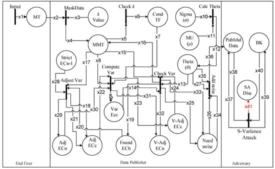
Figure 2.
HLPN for -sensitive k-anonymity.
Table 9.
Types used in HLPN for -sensitive k-anonymity.
Table 10.
Mapping of data types in -sensitive k-anonymity model.
The -sensitive k-anonymity algorithm was modeled through the HLPN rules for the microdata input. The data publisher initially verifies the k-value input. The original data is k-anonymized (bottom-up generalization) after finalizing the individual records in an EC obtained through variance calculations. In Rule (2), the k-anonymity masks the data. In Rule (2):
If an input k is less than the minimum size of an EC (i.e., <2) the condition fails. For cardinality having a minimum value of 2 or above, the algorithm executes. The k-anonymity for true or false are depicted in Rule (3).
The threshold is calculated in Rule (4). Variance for a fully diverse ECs for a specific k is calculated using the function. The important contributed functions are and functions, through which the algorithm processes all ECs. Transition performs all these swapping and noise additions in corresponding ECs. In Rule (5), transitions for the initial ECs. For the rest of the ECs, the same transition can be used in the same manner. In Rule (4):
In Rule (5):
The -sensitive k-anonymity model’s main functionalities are described in Rule (6) and Rule (7). Variance in each k-anonymous EC with respect to is checked in Rule (6). If variance of is greater than (i.e., ()), move to next and update the value in place MMT. If the variance of is less than (i.e., ), then transaction stops. We try to find , and swap required available values from . After performing all needed swapping, if the variance of is still less than (i.e., (), the noise is added to increase its diversity. In Rule (6):
The proposed -sensitive k-anonymity algorithm starts by processing each k size EC. The function computes the max frequency of , named as and , respectively. A one-way checking function: , checks for the existence of at that do not exist in earlier .
is swapped with after the checking succeeds and is saved in place Adj. minimizes the frequency of the value and increases diversity. While processing the last EC, i.e., , swapping is not possible in the forward direction. Thus swapping with previous EC is performed with a condition that the variance of already processed should not be decreased with . The function confirms two-way checking, that the values for both and are distinct and it should not change the variance of at place to an undesired value again. In that case, we call it strict . In other words, in addition to increasing the diversity in , it is also not increasing the frequency of value at place . Values are then swapped and are saved at place . Rule (7) shows the whole process. In Rule (7):
If the variance of is still less than (i.e., ), a dummy record called noise is added whenever needed throughout the variance adjustment process. In Rule (8), we have given the final noise addition case for last . Its purpose is to increase the variance at a level greater than . It will produce a highly diverse EC even if there are not enough diverse records in MMT. In Rule (8):
In Rule (9), an adversary attacks against the individual’s values. Adversary combines the already available BK (i.e., ) with the published data (i.e., ) and performs attack to disclose the patient’s identity (i.e., ) and the sensitive values (i.e., ). -sensitive k-anonymity model can provide better privacy protection to prevent from attribute disclosure attacks because it considers the high value of variance due to swapping and noise addition in corresponding ECs. The diversity of sensitive attribute values in ECs prevents the adversarial BK and is more effective as compared to the p+-sensitive k-anonymity model. Therefore, the adversary did not get private information for the target individual and the attack results in a null value. In Rule (9):
6. Experimental Evaluation
In this section, the experiments that were performed to show the effectiveness of the proposed -sensitive k-anonymity privacy model in comparison to the p+-sensitive k-anonymity model are described. The proposed algorithm wisely diversified the AS values in a balanced way inside each EC without using the categorical approach. The utility and quality of the anonymized released data were checked with numerous quality measures.
6.1. Experimental Setup
All experiments were performed on a machine with an Intel Core i5 2.39 GHz processor with 4 GB RAM, using the Windows 10 operating system. The algorithm was written in Python 3.7. We used the Adults database, which contained age, zip code, salary, and occupation attributes, which is openly accessible at the UC Irvine Machine Learning Repository, https://archive.ics.uci.edu/ml/datasets. We considered the age, zip code, salary as and occupation as .
Experimental results show the usefulness of the proposed -sensitive k-anonymity privacy model and protection against the categorical similarity attack and sensitive variance attack as compared to the p+-sensitive k-anonymity model. The quality of the sanitized publicly released data was evaluated with four utility metrics: discernibility penalty (DCP) [18,38,39], normalized average QI-group (CAVG) [17,18,38], noise calculation, and query accuracy [18,33]. The execution time of both algorithms was analyzed at the end of the experiments.
6.2. Discernibility Penalty (DCP)
The DCP proposed in [38] and used in [18,39] is an assignment of penalty (cost) to each tuple in the generalized data set. Through this penalty, the sanitized tuple cannot be distinguished among other tuples in the result set. Minimizing the discernibility cost is an optimal objective. The penalty for a tuple t that belongs to an EC of size |EC|, i.e., , will be |EC| and the penalty for each EC is . The complete DCP penalty for the overall sanitized released dataset can be seen in Equation (2).
where are the total number of ECs in . A baseline can be obtained from the most optimal DCP score calculations as shown in [10]. For example, if k = 2 and the number of anonymized tuples are 10, the DCP optimal score will be . This optimal score is called the baseline. The approach to generate groups followed in this paper was based on k size, inclusive of the noise tuple(s). Higher k means bigger group size, so the baseline moves up because of a high DCP score. The p+-sensitive k-anonymity model generated groups based on p. It means the number of tuples can be greater than p in a k-anonymous class. Figure 3 shows the DCS score for -sensitive k-anonymity, including a comparison with p+-sensitive and baseline. In comparison to p+-sensitivity, the DCP score, through the proposed -sensitive k-anonymity algorithm, is almost equal to the baseline, which implies that the proposed model assigned an optimal penalty to each EC and produced an optimal DCP score. The magnified subplots in Figure 3 with k = 12 and k = 16 for -sensitive k-anonymity shows the very minor difference with baseline. This minor difference can also be seen in Table 11, with an average DCP score of 47.2 or 0.002679% with a baseline obtained from the simulation while calculating the DCP for the anonymized dataset .
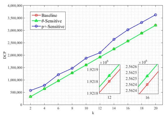
Figure 3.
Discernibility penalty (DSP) score.
Table 11.
DCP experiment values for each k.
6.3. Normalized Average (CAVG)
CAVG is another mathematically sound measurement that measures the quality of the sanitized data by the EC average size. It was proposed in [38] and applied in [17,18]. Below in Equation (3), CAVG can be calculated as
where is the overall sanitized released dataset and are the total number of ECs in . Data utility and CAVG are inversely proportional. Low CAVG value indicates high information utility. The optimal goal is to have a minimum size of ECs in . Figure 4 shows CAVG for p+-sensitive k-anonymity and -sensitive k-anonymity over k-anonymity. p+-sensitive has lower data utility over small k, where there is a high data utility for large k. The proposed technique has a very balanced and sustainable utility for each input value of k. Thus, the proposed -sensitive k-anonymity model performs efficiently for all sizes of k, compared to the p+-sensitive k-anonymity model.
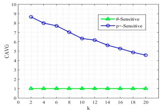
Figure 4.
The ratio of CAVG.
6.4. Noise Addition
Among different masking methods, one popular approach is the perturbation of data, i.e., noise addition. These are dummy tuples, added to the original data that helps in achieving the required diversity similar to the differential privacy [22,23]. The reason is if there are not enough values to swap with, especially in the second last and last ECs, the gap is filled with the noise tuples to prevent with disclosure risk. So, one of the reasons for such a good performance of the proposed model is the cost of noise addition. Figure 5 shows the number of tuples added as a noise for different values of k. These tuples are added to achieve the required value of the threshold . For different values of k, the algorithm responds differently but the maximum number of noise tuples added for a specific value of k is only six tuples. In the processed “Adult” dataset, the total number of tuples was 160,150 and only 34 noise tuples, i.e., 0.021% of the total size, were added in total. Such an amount of utility loss is negligible. This small amount of noise addition is sometimes due to get a round number when dividing the dataset size by the k size input, for example, 160150/4 = 40037.5 and 160152/4 = 40038.
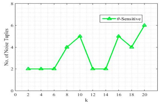
Figure 5.
The number of noise tuples added against each k.
6.5. Query Accuracy
Query accuracy measures precision for aggregate queries to check the utility of the anonymized data. It has been used by various research works [18,33]. To answer the aggregate queries, the built-in COUNT operator is used, where s are the query predicates. Consider to be a sanitized release from original microdata having maximum m as s (, where is the domain of ith QI. The SQLQuery in Equation (4) for the COUNT query will work as
Against each query, at least one or a few number of tuples should be selected from each EC based on query predicates. Two important parameters for query predicates are (1) query dimensionality q, and (2) the query selectivity . Query dimensionality comprises of the number of QIs in query predicate while query selectivity is the number of values for each attribute . The query selectivity is calculated as, , where are the output number of tuples after using query Q on relation R, and are the total number of tuples in the whole dataset. Query error i.e., Error(Q), is calculated in Equation (5).
where depicts result set from the COUNT query on an anonymized dataset while is the result set from the COUNT query on the original microdata. More selective queries have a high error rate.
Figure 6a shows the query error for the input value of k. We compare the p+-sensitive k-anonymity and -sensitive k-anonymity using the query error rate for 1000 randomly generated aggregate queries. The error rate increases for the high value of k because of the high range in s. This selects a greater number of tuples than the original microdata and hence high error rate. In Figure 6b, it is depicted that the more we select tuples based on predicates, the higher the error rate will be in the anonymized data.
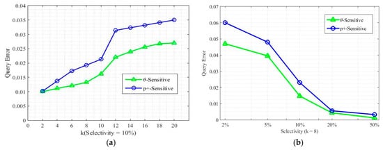
Figure 6.
(a) Query error for k. (b) Query error for selectivity.
6.6. Execution Time
Figure 7 shows the execution time for both p+-sensitive k-anonymity model and for the proposed -sensitive k-anonymity model. The execution time for both of the algorithms increased with an increase in value of k because of the increase in generalization range. Since we did not consider the sensitive values categorization, our approach took a small amount of time to execute as compared to its counterpart. In the -sensitive k-anonymity model, a higher execution time for k = 10, k = 16 and k = 20 was because of the time taken to add more noise tuples to achieve the required diversity.
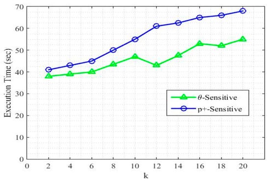
Figure 7.
Algorithm execution time.
7. Conclusions
In this paper, the huge amount of data (i.e., Big Data) collected through the IoT-based devices were anonymized using the proposed -sensitive k-anonymity privacy model in comparison to p+-sensitive k-anonymity model. The purpose was to prevent an attribute disclosure risk in anonymized data. The p+-sensitive k-anonymity model was considered to be vulnerable to a privacy breach from sensitive variance, categorical similarity, and homogeneity attacks. These attacks were mitigated by implementing the proposed -sensitive k-anonymity privacy model using Equation (1). In the proposed solution, the threshold value decides the diversity level for each EC of the dataset. The vulnerabilities in the p+-sensitive k-anonymity model and the effectiveness of the proposed -sensitive k-anonymity model were formally modeled through HLPN, which further ensures the validation of the proposed technique. The experimental work proved the privacy implementation and an improved utility of the released data using different mathematical measures. For future work consideration, the proposed algorithm can be extended to 1:M (single record having many attribute values) [40], to multiple sensitive attributes (MSA) [41,42,43], or can be modeled by considering the dynamic data set [44] approach.
Author Contributions
Conceptualization, R.K. and X.T.; methodology, R.K., X.T., and A.A.; software, R.K.; validation, X.T. and A.A.; formal analysis, R.K., T.K., and S.u.R.M.; writing—original draft preparation, T.K.; writing—review and editing, T.K., X.T., A.A., A.K., W.u.R., and C.M.; supervision, X.T.; funding acquisition, X.T. All authors have read and agreed to the published version of the manuscript.
Funding
This work was supported by the National Natural Science Foundation of China (61932005), and 111 Project of China B16006.
Conflicts of Interest
The authors declare that there is no conflict of interests regarding the publication of this paper.
References
- Dang, L.M.; Piran, J.; Han, D.; Min, K.; Moon, H. A Survey on Internet of Things and Cloud Computing for Healthcare. Electronics 2019, 8, 768. [Google Scholar] [CrossRef]
- Sun, W.; Cai, Z.; Li, Y.; Liu, F.; Fang, S.; Wang, G. Security and Privacy in the Medical Internet of Things: A Review. Secur. Commun. Netw. 2018, 2018, 1–9. [Google Scholar] [CrossRef]
- Baek, S.; Seo, S.-H.; Kim, S.J. Preserving Patient’s Anonymity for Mobile Healthcare System in IoT Environment. Int. J. Distrib. Sens. Netw. 2016, 12, 2171642. [Google Scholar] [CrossRef][Green Version]
- Liu, F.; Li, T. A Clustering K-Anonymity Privacy-Preserving Method for Wearable IoT Devices. Secur. Commun. Netw. 2018, 2018, 1–8. [Google Scholar] [CrossRef]
- Wan, J.; Al-Awlaqi, M.A.A.H.; Li, M.; O’Grady, M.; Gu, X.; Wang, J.; Cao, N. Wearable IoT enabled real-time health monitoring system. EURASIP J. Wirel. Commun. Netw. 2018, 2018, 298. [Google Scholar] [CrossRef]
- Al-Khafajiy, M.; Baker, T.; Chalmers, C.; Asim, M.; Kolivand, H.; Fahim, M.; Waraich, A. Remote health monitoring of elderly through wearable sensors. Multimed. Tools Appl. 2019, 78, 24681–24706. [Google Scholar] [CrossRef]
- Sweeney, L. k-anonymity: A model for protecting privacy. Int. J. Uncertain. Fuzziness Knowl. Based Syst. 2002, 10, 557–570. [Google Scholar] [CrossRef]
- Sweeney, L. Achieving k-anonymity privacy protection using generalization and suppression. Int. J. Uncertain. Fuzziness Knowl. Based Syst. 2002, 10, 571–588. [Google Scholar] [CrossRef]
- Song, F.; Ma, T.; Tian, Y.; Al-Rodhaan, M. A New Method of Privacy Protection: Random k-Anonymous. IEEE Access 2019, 7, 75434–75445. [Google Scholar] [CrossRef]
- Wang, J.; Du, K.; Luo, X.; Li, X. Two privacy-preserving approaches for data publishing with identity reservation. Knowl. Inf. Syst. 2018, 60, 1039–1080. [Google Scholar] [CrossRef]
- Amiri, F.; Yazdani, N.; Shakery, A.; Chinaei, A.H. Hierarchical anonymization algorithms against background knowledge attack in data releasing. Knowl. Based Syst. 2016, 101, 71–89. [Google Scholar] [CrossRef]
- Yaseen, S.; Abbas, S.M.A.; Anjum, A.; Saba, T.; Khan, A.; Malik, S.U.R.; Ahmad, N.; Shahzad, B.; Bashir, A.K. Improved Generalization for Secure Data Publishing. IEEE Access 2018, 6, 27156–27165. [Google Scholar] [CrossRef]
- Liu, X.; Deng, R.H.; Choo, K.K.R.; Weng, J. An efficient privacy preserving outsourced calculation tool kit with multiple keys. IEEE Trans. Inf. Forensics Secur. 2016, 11, 2401–2414. [Google Scholar] [CrossRef]
- Michalas, A. The lord of the shares. In Proceedings of the 34th ACM/SIGAPP Symposium on Applied Computing, Limassol, Cyprus, 8–12 April 2019; pp. 146–155. [Google Scholar] [CrossRef]
- Machanavajjhala, A.; Gehrke, J.; Kifer, D.; Venkitasubramaniam, M. L-diversity: Privacy beyond k-anonymity. Int. Conf. Data Eng. 2006, 1, 24. [Google Scholar] [CrossRef]
- Li, N.; Li, T.; Venkatasubramanian, S. t-Closeness: Privacy beyond k-Anonymity and l-Diversity. In Proceedings of the 2007 IEEE 23rd International Conference on Data Engineering, Istanbul, Turkey, 15–20 April 2007; pp. 106–115. [Google Scholar]
- Sun, X.; Sun, L.; Wang, H. Extended k-anonymity models against sensitive attribute disclosure. Comput. Commun. 2011, 34, 526–535. [Google Scholar] [CrossRef]
- Anjum, A.; Malik, S.U.R.; Choo, K.-K.R.; Khan, A.; Haroon, A.; Khan, S.; Khan, S.U.; Ahmad, N.; Raza, B. An efficient privacy mechanism for electronic health records. Comput. Secur. 2018, 72, 196–211. [Google Scholar] [CrossRef]
- Campan, A.; Truta, T.M.; Cooper, N. p-sensitive k-anonymity with generalization constraints. Trans. Data Privacy 2010, 3, 65–89. [Google Scholar]
- Al-Khafajiy, M.; Webster, L.; Baker, T.; Waraich, A. Towards fog driven IoT healthcare. In Proceedings of the 2nd International Conference on Future Networks and Distributed Systems, Amman, Jordan, 26–27 June 2018; Volume 9, p. 9. [Google Scholar]
- Shahzad, A.; Lee, Y.S.; Lee, M.; Kim, Y.-G.; Xiong, N.N. Real-Time Cloud-Based Health Tracking and Monitoring System in Designed Boundary for Cardiology Patients. J. Sens. 2018, 2018, 1–15. [Google Scholar] [CrossRef]
- Domingo-Ferrer, J.; Soria-Comas, J. From t-closeness to differential privacy and vice versa in data anonymization. Knowl. Based Syst. 2015, 74, 151–158. [Google Scholar] [CrossRef]
- Dwork, C. Differential privacy. In International Colloquium on Automata, Languages, and Programming; Springer: Berlin/Heidelberg, Germany, 2006; pp. 1–12. [Google Scholar]
- Fung, B.C.; Wang, K.; Chen, R.; Yu, P.S. Privacy-preserving data publishing. ACM Comput. Surv. 2010, 42, 1–53. [Google Scholar] [CrossRef]
- Xu, Y.; Ma, T.; Tang, M.; Tian, W. A Survey of Privacy Preserving Data Publishing using Generalization and Suppression. Appl. Math. Inf. Sci. 2014, 8, 1103–1116. [Google Scholar] [CrossRef]
- Torra, V. Transparency in Microaggregation; UNECE: Skovde, Sweden, 2015; pp. 1–8. Available online: http://www.diva-portal.org/smash/record.jsf?pid=diva2%3A861563&dswid=-2982 (accessed on 25 August 2019).
- Panackal, J.J.; S.Pillai, A. Adaptive Utility-based Anonymization Model: Performance Evaluation on Big Data Sets. Procedia Comput. Sci. 2015, 50, 347–352. [Google Scholar] [CrossRef]
- Rahimi, M.; Bateni, M.; Mohammadinejad, H. Extended K-Anonymity Model for Privacy Preserving on Micro Data. Int. J. Comput. Netw. Inf. Secur. 2015, 7, 42–51. [Google Scholar] [CrossRef]
- Sowmiyaa, P.; Tamilarasu, P.; Kavitha, S.; Rekha, A.; Krishna, G.R. Privacy Preservation for Microdata by using k-Anonymity Algorthim. Int. J. Adv. Res. Comput. Commun. Eng. 2015, 4, 373–375. [Google Scholar]
- Wong, C.; Li, J.; Fu, W.; Wang, K. (α,k)-Anonymity: An enhanced k-anonymity model for privacy preserving data publishing. In Proceedings of the 12th ACM SIGKDD international conference on Knowledge discovery and data mining ACM, Philadelphia, PA, USA, 20–23 August 2006; pp. 754–759. [Google Scholar]
- Zhang, Q.; Koudas, N.; Srivastava, D.; Yu, T. Aggregate Query Answering on Anonymized Tables. In Proceedings of the 2007 IEEE 23rd International Conference on Data Engineering, Institute of Electrical and Electronics Engineers (IEEE), Istanbul, Turkey, 17–20 April 2007; pp. 116–125. [Google Scholar]
- Li, J.; Tao, Y.; Xiao, X. Preservation of proximity privacy in publishing numerical sensitive data. In Proceedings of the 2008 ACM SIGMOD International Conference, Association for Computing Machinery (ACM), Vancouver, BC, Canada, 9–12 June 2008; pp. 473–486. [Google Scholar] [CrossRef]
- Xiao, X.; Tao, Y. Personalized privacy preservation. In Proceedings of the 2006 ACM SIGMOD International Conference, Chicago, IL, USA, 27–29 June 2006; p. 229. [Google Scholar] [CrossRef]
- Christen, P.; Vatsalan, D.; Fu, Z. Advanced Record Linkage Methods and Privacy Aspects for Population Reconstruction—A Survey and Case Studies. In Population Reconstruction; Springer: Berlin, Germany, 2015; pp. 87–110. [Google Scholar] [CrossRef]
- Kullback, S.; Leibler, R.A. On Information and Sufficiency. Ann. Math. Stat. 1951, 22, 79–86. [Google Scholar] [CrossRef]
- Rubner, Y.; Tomasi, C.; Guibas, L.J. The Earth Mover’s Distance as a Metric for Image Retrieval. Int. J. Comput. Vis. 2000, 40, 99–121. [Google Scholar] [CrossRef]
- Ali, M.; Malik, S.U.R.; Khan, S.U. DaSCE: Data Security for Cloud Environment with Semi-Trusted Third Party. IEEE Trans. Cloud Comput. 2015, 5, 642–655. [Google Scholar] [CrossRef]
- Bayardo, R.J.; Agrawal, R. Data Privacy through Optimal k-Anonymization. In Proceedings of the 21st International Conference on Data Engineering (ICDE’05), Tokyo, Japan, 5–8 April 2005; pp. 217–228. [Google Scholar]
- Lefevre, K.; DeWitt, D.; Ramakrishnan, R. Mondrian Multidimensional K-Anonymity. In Proceedings of the 22nd International Conference on Data Engineering, Atlanta, GA, USA, 3–8 April 2006; p. 25. [Google Scholar]
- Gong, Q.; Luo, J.; Yang, M.; Ni, W.; Li, X.-B. Anonymizing 1:M microdata with high utility. Knowl. Based Syst. 2016, 115, 15–26. [Google Scholar] [CrossRef]
- Wang, R.; Zhu, Y.; Chen, T.-S.; Chang, C.-C. Privacy-Preserving Algorithms for Multiple Sensitive Attributes Satisfying t-Closeness. J. Comput. Sci. Technol. 2018, 33, 1231–1242. [Google Scholar] [CrossRef]
- Anjum, A.; Ahmad, N.; Malik, S.U.R.; Zubair, S.; Shahzad, B. An efficient approach for publishing microdata for multiple sensitive attributes. J. Supercomput. 2018, 74, 5127–5155. [Google Scholar] [CrossRef]
- Khan, R.; Tao, X.; Anjum, A.; Sajjad, H.; Malik, S.U.R.; Khan, A.; Amiri, F. Privacy Preserving for Multiple Sensitive Attributes against Fingerprint Correlation Attack Satisfying c-Diversity. Wirel. Commun. Mob. Comput. 2020, 2020, 1–18. [Google Scholar] [CrossRef]
- Zhu, H.; Liang, H.B.; Zhao, L.; Peng, D.Y.; Xiong, L. τ-Safe (l,k)-Diversity Privacy Model for sequential publication with high utility. IEEE Access 2019, 7, 687–701. [Google Scholar] [CrossRef]
© 2020 by the authors. Licensee MDPI, Basel, Switzerland. This article is an open access article distributed under the terms and conditions of the Creative Commons Attribution (CC BY) license (http://creativecommons.org/licenses/by/4.0/).