


Abstract
To address the difficulty of simultaneously achieving fast response, high stability, and strong disturbance rejection in gimbal systems operating under complex conditions, an adaptive control strategy based on offline–online cooperative optimization is proposed. The method is built upon the conventional proportional–integral–derivative (PID) control framework. First, a particle swarm optimization (PSO) algorithm is employed offline to obtain an optimized set of initial control parameters, thereby improving the transient response during the startup phase. Subsequently, a single-neuron adaptive (SNA) mechanism is introduced to adjust the control parameters online according to real-time error information, enhancing the system’s adaptability to environmental variations and external disturbances. Stability analysis demonstrates the convergence of the proposed control scheme. Finally, an experimental gimbal platform is constructed to validate the effectiveness of the method. Experimental results show that, under various disturbance conditions, the proposed strategy effectively reduces angular fluctuation amplitude, shortens the settling time, and maintains smooth control performance. These results indicate that the proposed control strategy exhibits strong robustness and significant engineering applicability.
1. Introduction
As a critical actuator carrying imaging equipment, the gimbal system has become a core device for improving the visual quality of mobile imaging by compensating for carrier-induced vibration errors in real time. Gimbal systems are widely used in dynamic imaging scenarios such as agricultural plant protection and power line inspection [1,2,3,4], where they can replace manual operations in heavy and repetitive inspection tasks, thereby significantly improving operational efficiency [5,6,7,8]. To meet the requirements of high-quality imaging, mitigating image blur caused by vibration has become a key technical challenge. Current mainstream solutions can be broadly classified into three categories.
(1) Video post-processing stabilization, in which camera motion is first estimated from image sequences and the image frames are continuously warped to achieve visual stabilization.
(2) Mechanical stabilization, which relies on mechanical structures such as damping springs to minimize camera vibration during recording.
(3) Active motor-based stabilization, where the camera attitude is adjusted through motor control to counteract external disturbances and stabilize the captured image.
Based on the third approach, Qianwen Duan et al. [9], Aytaç Altan et al. [10], and Franz Königseder et al. [11] designed stabilized gimbal systems that employ sensors to acquire real-time attitude information and correct the camera pose through motor control, thereby maintaining image clarity. However, with increasing mechanical complexity and higher demands on image quality, more stringent requirements are imposed on the control strategies of stabilized gimbals.
A wide range of control algorithms has been proposed for gimbal systems. Traditional proportional–integral–derivative (PID) control methods do not require accurate system modeling and have, therefore, been widely adopted in practical applications [12,13]. However, purely feedback-based control algorithms such as PID exhibit inherent limitations in meeting high requirements for positioning accuracy and fast dynamic response [14]. Their robustness is relatively weak, and their disturbance rejection capability is insufficient. To improve system robustness, some studies have introduced sliding-mode control (SMC) [15,16]. Although SMC theoretically offers strong robustness against uncertainties, its control performance is sensitive to model accuracy and parameter matching. In addition, chattering phenomena are often unavoidable, which increases implementation difficulty in practical embedded gimbal systems. Active disturbance rejection control (ADRC) has been proposed to estimate and compensate for internal and external disturbances, thereby reducing reliance on precise system models to a certain extent [17,18,19]. Nevertheless, ADRC controllers typically involve a large number of parameters, and their tuning procedures are largely dependent on experience. The mapping between parameters and control performance is not intuitive, resulting in high engineering tuning costs and cumbersome parameter adjustment processes. To address the tuning difficulty of ADRC, linear active disturbance rejection control (LADRC) was proposed in [20], and the bandwidth-based method has gradually become the mainstream approach for LADRC parameter tuning [21]. Although parameter selection methods for linear extended state observers have been reported [22], the tuning of ADRC-based controllers remains challenging in practice. Trade-offs among observer bandwidth, control bandwidth, and noise suppression are still required, and parameter selection has a significant impact on system performance. In comparison, PID control methods incorporating intelligent optimization and lightweight adaptive mechanisms provide a more favorable balance between engineering implementation complexity and control performance.
To enhance robustness against modeling uncertainties and external disturbances, an intelligent PID controller for robotic manipulators was presented [23]. A neural network-based PID controller with self-learning capability was proposed; however, information interaction among multiple neurons introduces time delays resulted in limited real-time performance during training [24]. Neural network (NN) adaptive control approaches were investigated, but only simulation results were provided, without implementation on physical hardware [25,26]. In contrast, the single-neuron adaptive PID control strategy proposed in [27] demonstrates strong self-learning and adaptive capabilities, while also exhibiting superior stability and real-time performance when applied to nonlinear time-varying systems.
Although neural networks offer online learning and nonlinear approximation capabilities, multilayer neural networks are characterized by complex structures and large parameter sets, making them difficult to deploy reliably in real-time control systems or embedded platforms. Considering the computational and memory constraints of microcontroller units (MCUs), this study adopts a single-neural adaptive approach as the online adaptive algorithm for tuning PID controller parameters. This strategy significantly simplifies parameter tuning while enabling real-time adjustment in response to external disturbances. In addition, PSO has been employed to optimize PID parameters through iterative searching, and experimental results on robotic arm vibration demonstrate improved vibration suppression compared with conventional methods [28]. This study further integrates the global optimization capability of PSO with the online adaptive characteristics of the SNA mechanism to develop a hybrid control strategy for embedded gimbal systems, achieving a balanced trade-off among control performance, parameter tunability, and practical implementability.
This paper proposes an offline–online cooperative adaptive PID strategy for gimbal stabilization that combines PSO-based offline pre-tuning with a single-neuron online adaptation mechanism. The offline PSO stage is used only to provide conservative and stable initialization on a simplified surrogate model, avoiding unsafe parameter exploration on hardware, while the online single-neuron mechanism continuously compensates for time-varying disturbances and aggregated uncertainties during operation. A projection-based bounding mechanism is incorporated to prevent parameter drift and improve implementation safety on resource-constrained embedded platforms. The proposed method is validated on a physical single-axis gimbal under multiple disturbance and reference-change scenarios.
The remainder of this paper is organized as follows. Section 2 presents the mathematical model of the gimbal system. Section 3 describes the construction of the adaptive PID control strategy based on offline–online cooperative optimization. Section 4 introduces the implementation of the gimbal system. Section 5 provides experimental analysis of the proposed algorithm. Section 6 concludes the paper.
2. Mathematical Modeling of the Gimbal System
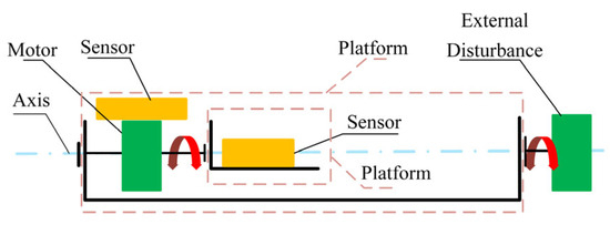
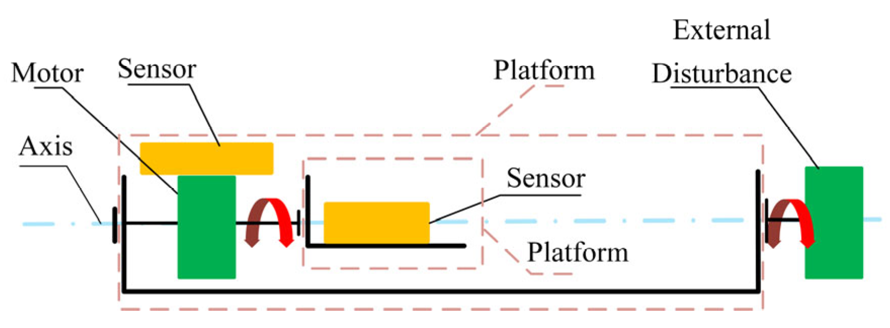
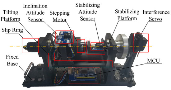
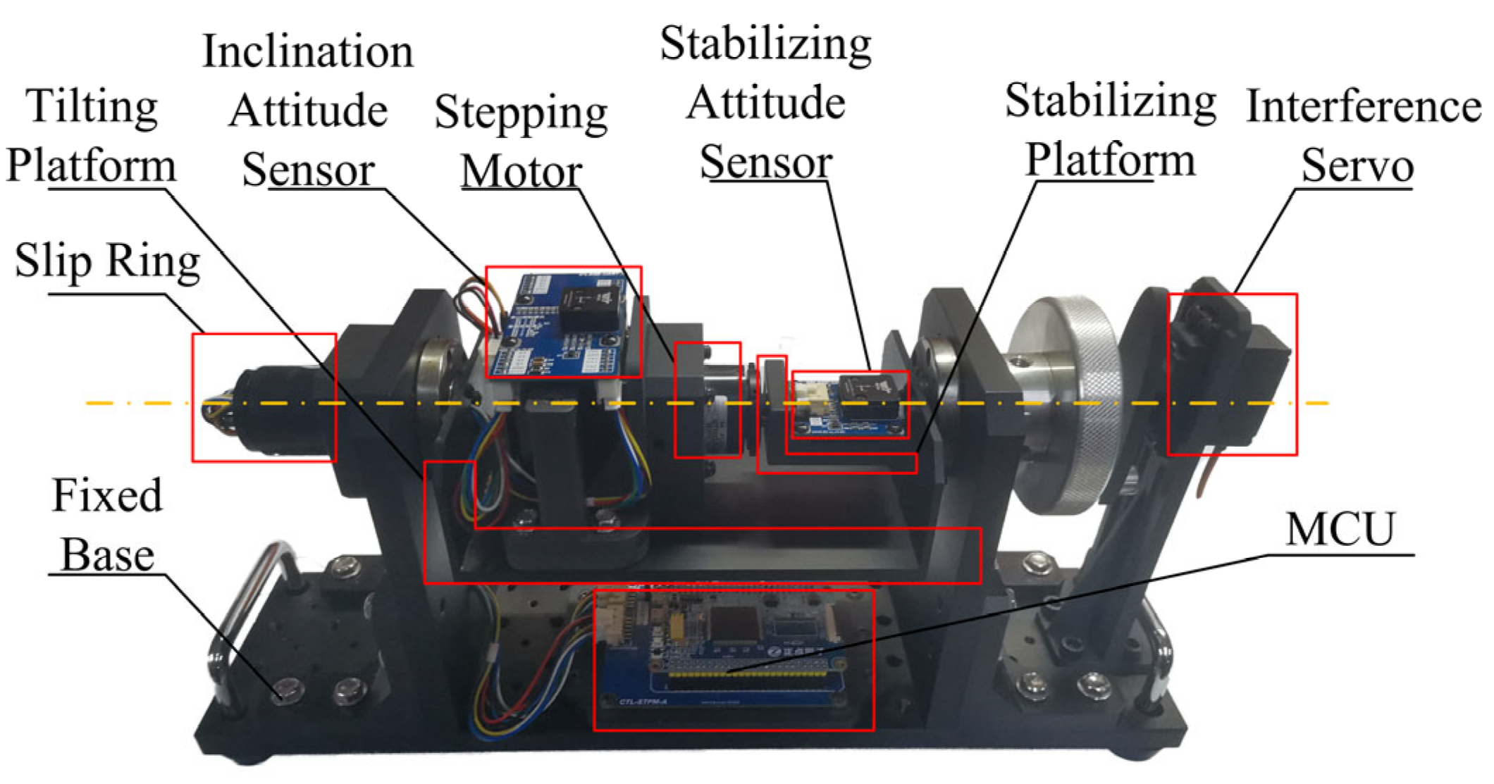
The gimbal system investigated in this study is a self-designed and experimentally constructed platform. A structural schematic of the experimental gimbal is illustrated in Figure 1. The system mainly consists of sensors, an actuating motor, disturbance-generating components, a fixed platform, and a microcontroller. Sensor measurements are acquired and processed by the microcontroller, where the control algorithm is executed. Based on the control outputs, the actuating motor adjusts the motion of the controlled object to maintain system stability.
Figure 1.
Experimenter mechanical vector drawing.
To ensure precise control performance, a stepper motor is selected as the actuating element of the gimbal system. To prevent step loss during operation, a position closed-loop control scheme is adopted at the low-level motor drive layer of the experimental platform. The back electromotive force (back-EMF) of the phase windings of the stepper motor can be expressed as follows:
where and denote the back electromotive forces of the A-phase and B-phase windings of the stepper motor, respectively; is the rotor angular velocity; represents the number of rotor teeth; is the back-EMF coefficient; and denotes the mechanical rotation angle of the rotor.
The instantaneous electromagnetic torque of the stepper motor is given by the following:
where and are the currents of the A-phase and B-phase windings, respectively.
According to the kinematic equation, the relationship between the electromagnetic torque and the load torque can be expressed as follows:
where denotes the total rotational inertia of the motor rotor and the gimbal arm, is the viscous damping coefficient, and represents the load torque.
To simplify the analysis, a single-phase excitation mode and a no external load condition () are considered. The motor motion equations are linearized around the equilibrium point and transformed into the Laplace domain, allowing the controlled object to be approximated as a second-order system.
It should be noted that stepper motors inherently exhibit nonlinear and hybrid characteristics, and their dynamic behavior is jointly influenced by cogging torque, magnetic flux nonlinearity, resonance regions, and discrete stepping effects. The second-order linear model adopted in this study is not intended to accurately capture the complete dynamics of the stepper motor, but rather to serve as an equivalent approximation in the vicinity of a nominal operating point. The primary purpose of this model is to provide a stable and computationally tractable environment for offline parameter pre-tuning using the particle swarm optimization algorithm, thereby avoiding potential safety risks associated with large-scale parameter searches conducted directly on physical hardware. Consequently, this study does not aim to reproduce the full-range dynamic response of the stepper motor using the linear model, and the discrepancies between the model and the actual system are regarded as part of the unmodeled dynamics and equivalent disturbances. For the 42ZDT40A stepper motor used in this study, the equivalent transfer function obtained around the operating point of the experimental platform is given by the following:
where is the input reference angle and is the actual output angle. The motor parameters are listed in Table 1.
Table 1.
42ZDT40A motor parameters.
It should be emphasized that the second-order linear transfer function is adopted only as a simplified and computationally convenient surrogate model for the offline parameter pre-tuning stage. The stepper motor inherently exhibits nonlinear and hybrid characteristics that cannot be fully captured by this linear approximation. In the present study, these unmodeled nonlinearities are treated as aggregated uncertainties and equivalent disturbances in the closed-loop system. The proposed online single-neuron adaptive mechanism is designed to mitigate such effects based on real-time tracking errors, while the offline PSO stage serves only to provide a reasonable and stable initial parameter set for controller initialization.
3. Construction of an Adaptive PID Control Strategy Based on Offline–Online Cooperative Optimization
3.1. Single-Neuron Online Adaptive Mechanism
Conventional proportional–integral–derivative (PID) controllers are widely adopted due to their simple structure and strong engineering applicability. However, their control performance is highly dependent on parameter tuning. When the controlled system exhibits parameter uncertainties, operating condition variations, or external disturbances, fixed-parameter PID controllers often fail to simultaneously achieve satisfactory dynamic and steady-state performance.
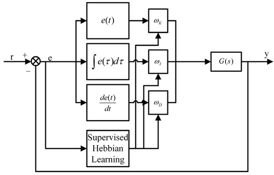
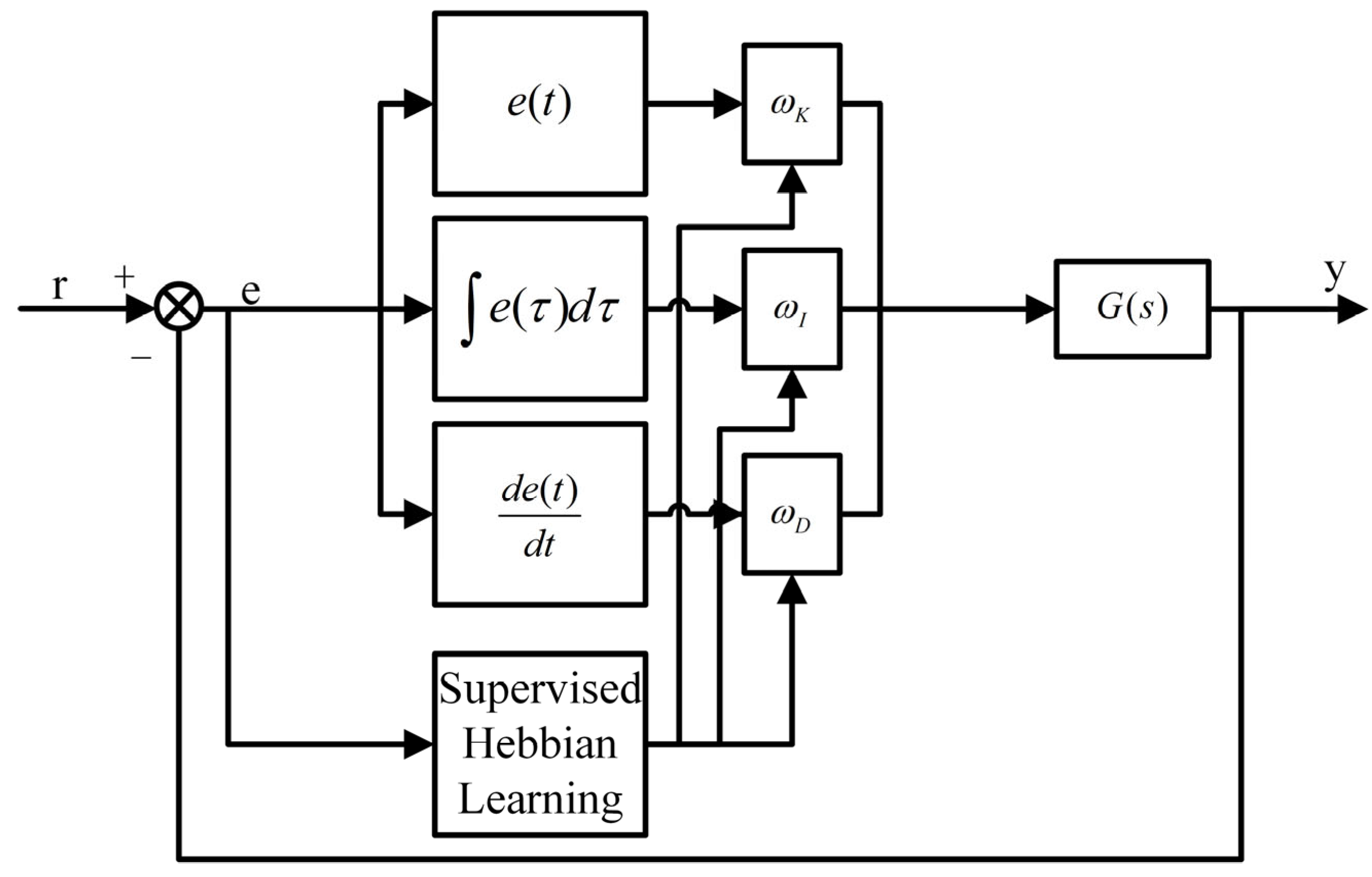
To address this limitation, a single-neuron model is introduced as an adaptive mechanism. This approach preserves the physical structure and interpretability of the PID controller while enabling online parameter adjustment. In addition, the single-neuron structure is computationally lightweight and can be conveniently deployed on microcontroller-based platforms, making it suitable for real-time control applications. The basic architecture of the single-neuron adaptive PID control strategy is illustrated in Figure 2.
Figure 2.
Single-neuron adaptive PID control strategy.
3.2. Single-Neuron Equivalent Form of the Incremental PID Controller
The tracking error is defined as follows:
where denotes the reference input, is the system output, and represents the discrete time instant.
The three feature inputs of the incremental PID controller are selected as follows [29]:
The weight vector of the single neuron is defined as follows:
where , and correspond to the equivalent gains of the proportional, integral, and derivative channels, respectively. To prevent unbounded growth of the weights while preserving their relative proportions, normalized weights are introduced as follows:
where , as a small positive constant, is introduced to avoid a zero denominator.
Accordingly, the control increment can be expressed in the single-neuron form as follows:
The controller output is then obtained by , where is a global scaling factor used to adjust the control action intensity.
3.3. Supervised Hebbian Learning Rule
The output of the single neuron is defined as follows:
where denotes the output threshold of the single neuron, which is set to zero in this study.
The supervised Hebbian learning rule is adopted as follows [30]:
where is the learning rate and represents the desired output.
The supervisory signal can be constructed from the tracking error. To ensure that the weight update directly serves error convergence, the following supervisory signal is selected in this study:
By associating the neuron output with the controller output, an implementable online weight update law is obtained as follows:
To guarantee boundedness of the weights and enhance system stability, a projection operator is introduced as follows:
where is the diagonal learning-rate matrix, denotes the admissible weight constraint set, and the projection operator projects the updated weights onto the set .
3.4. Offline Pre-Tuning of PID Parameters Based on Particle Swarm Optimization
Although the single-neuron adaptive PID controller is capable of adjusting parameters online, its convergence performance is closely related to the selection of initial parameters. Inappropriate initial parameters not only prolong the online learning process but may also introduce a high risk of excessive overshoot or even instability during the system startup phase.
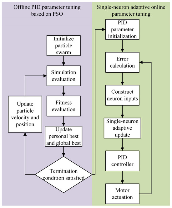
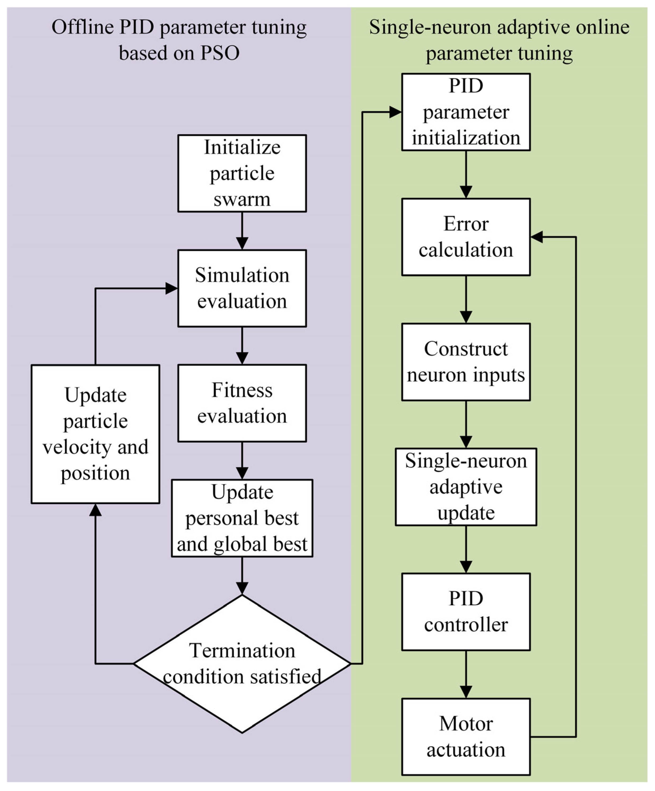
Therefore, prior to controller deployment, a particle swarm optimization (Particle Swarm Optimization, PSO) algorithm is introduced to perform offline tuning of the PID parameters. Through the global search conducted by PSO in the parameter space, a set of well-performing initial parameters (, , ) is obtained and written into the microcontroller as the initial weights for the subsequent single-neuron online adaptation. The offline–online cooperative optimization framework for PID parameter tuning is illustrated in Figure 3.
Figure 3.
Offline–online cooperative optimization framework for PID parameter tuning.
In the PSO algorithm, each particle corresponds to a candidate set of PID parameters, and its position vector is defined as follows:
To ensure physical feasibility and engineering stability during the search process, upper and lower bounds are imposed on each parameter as follows:
The particle swarm optimization algorithm guides the search process by exploiting both the personal best and the global best information. At the -th iteration, the velocity and position update rules of the -th particle are given by the following:
where denotes the particle velocity vector, is the personal best position of the particle, represents the global best position of the swarm, is the inertia weight, and are the learning factors, and , are uniformly distributed random numbers.
To prevent excessive particle velocity from causing instability in the search process, velocity clamping is applied as follows:
To jointly consider control accuracy and response speed, the integral of the time-weighted absolute error (ITAE) criterion is adopted as the fitness function of the PSO algorithm. In this study, the ITAE criterion is employed as a consistent performance index for offline parameter pre-tuning based on the simplified linear model. It should be noted that the PSO procedure is not intended to identify global optimal parameters for the actual hardware system. Rather, it is used to obtain a reasonable and stable initial parameter set that facilitates the subsequent online adaptive process. The ITAE index is defined as follows:
where denotes the system error and represents the simulation duration.
The PSO-tuned parameters solution obtained by PSO is as follows:
which is used as the initial PID parameters of the controller.
The parameters optimized offline by PSO are employed to initialize the weights of the single-neuron adaptive PID controller:
During system operation, PSO no longer participates in online control, and the PID parameters are updated exclusively through the single-neuron adaptive learning law based on real-time error information. Due to the stochastic nature of PSO, different runs may lead to slightly different parameter sets. In this study, PSO is used as an auxiliary offline tool for parameter pre-tuning, and minor variations in initialization do not affect the final conclusions, since the proposed online adaptive mechanism further adjusts the controller parameters during operation.
3.5. Lyapunov Stability Analysis
The PSO module is executed offline and does not participate in the online closed-loop dynamics after deployment. Therefore, the stability analysis focuses on the online adaptive law of the single-neuron PID controller, with the PSO stage affecting only the initial condition of the adaptive parameters. The following stability analysis is therefore conducted for the closed-loop system incorporating the single-neuron online adaptive law. Considering the nonlinear and time-varying characteristics of the plant, an incremental model around the operating point is employed for stability analysis. The discrete-time system output is assumed to satisfy the following commonly used equivalent gain assumption:
where denotes an unknown but bounded equivalent gain satisfying the following:
and represents the aggregated effect of unmodeled dynamics and external disturbances, which is bounded. In practice, the bounding of closed-loop signals is ensured by physical constraints (limited actuator authority and sensor ranges) and by software safeguards.
Based on the error definition , when the increment of the reference signal is bounded, the error dynamics can be expressed as follows:
where remains a bounded disturbance term.
Define the weight estimation error as , where denotes the ideal constant weight vector. The following Lyapunov candidate function is selected:
where .
From (24), the formula below is followed:
The error difference term satisfies the following identity:
and admits the upper bound
For the parameter-related terms, the projection operator is non-expansive and guarantees the boundedness of the weights, i.e., the projection operator is introduced as an implementation-oriented safeguard to prevent parameter drift and to avoid actuator saturation/instability on resource-constrained embedded hardware. Similar projection-based adaptive laws are widely used to guarantee bounded parameters in adaptive control [31]. . Under the update law (14), the difference of satisfies an inequality of the standard form:
where is related to and ; depends on the learning rate and the bounds of the involved signals; and is a positive constant.
If is bounded through saturation or filtering mechanisms, and the learning rate is selected such that , the following conclusions can be drawn:
When , , the closed-loop signals are bounded, and the tracking error converges to zero.
When is bounded, the system is uniformly ultimately bounded; that is, there exists a positive constant such that for sufficiently large , .
Moreover, due to the constraint imposed by the projection operator, the adaptive weights remain bounded throughout the operation.
4. Experimental System Construction and Implementation
The overall design of the experimental platform is illustrated in Figure 4. The system takes angular displacement and angular velocity as inputs. A microcontroller outputs position commands to the stepper motor driver, thereby controlling the pulse count driving the stepper motor.
Figure 4.
Vehicle-mounted stabilized gimbal system framework.
During system operation, two attitude sensors are employed to independently acquire the pose information of the tilting platform and the stabilizing platform. The measured data are fed back to the MCU in real time as control feedback signals. All the above components are mounted on a fixed base. The stepper motor is installed on the tilting platform and rotates synchronously with it. The tilting platform is rigidly connected to the servo horn, while the stabilizing platform is fixed to the output shaft of the stepper motor. All platforms rotate along the same axis.
Based on the acquired attitude data, the MCU executes the control algorithm and generates target position commands for the stepper motor to achieve stabilized platform position control. Finally, experimental data are transmitted to the PC via serial communication, where signal waveforms are displayed and analyzed for performance evaluation.
An STM32F103ZET6 microcontroller is used as the MCU of the system. Two internal USART interfaces are utilized to acquire pose data from the attitude sensors installed on the tilting platform and the stabilizing platform, respectively. PWM signals are generated through TIM channels to control the active disturbance servo motor, while another USART interface is used to perform micro-stepping control of the stepper motor. An RS232 interface is designed to communicate with the PC, enabling real-time transmission and visualization of the pose data of both platforms.
The HWT606 six-axis attitude sensor is selected for pose measurement. By acquiring three-axis acceleration, gyroscope, and magnetic field data, a Kalman filter-based sensor fusion algorithm is employed to estimate the three-axis angular information. When operating away from strong magnetic interference, the angle accuracy of the X- and Y-axes can reach 0.01°. The sensor supports a baud rate of up to 921,600, with a maximum data output rate of 1000 Hz, satisfying the requirements for high-rate sampling. In the sensor circuit design, protection circuits against overcurrent, overvoltage, and reverse polarity are incorporated to prevent electrical damage.
Considering that excessively large proportional or integral gains in embedded gimbal systems may lead to control output saturation, which can, in turn, cause abrupt increases in drive current, actuator vibration, or even system instability, appropriate gain limits are necessary. Preliminary experimental tests indicate that when , and exceed approximately 10, the system tends to exhibit pronounced high-frequency oscillations or control saturation phenomena. Therefore, this range is adopted as a conservative safety upper bound for the controller parameters in this study. The parameter settings of the PSO-based single-neuron PID controller are listed in Table 2.
Table 2.
PSO Parameters.
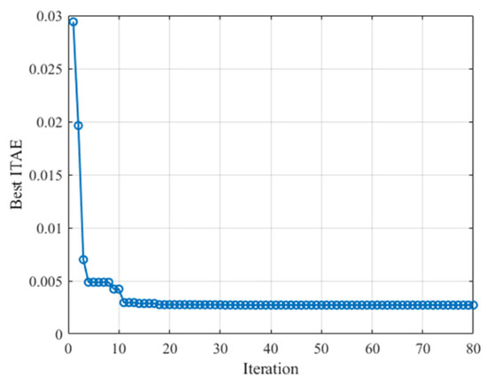
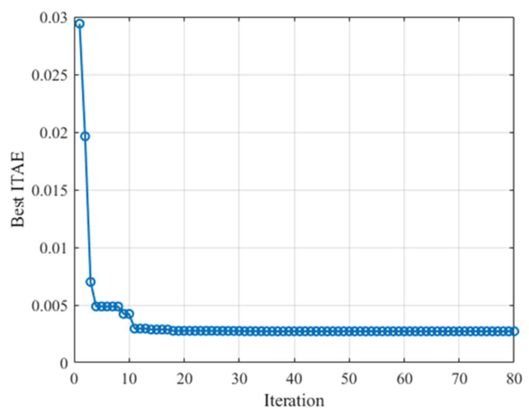
As a stochastic search method, the particle swarm optimization algorithm may yield slightly different optimization results under different initial random population conditions. In this study, PSO is primarily introduced to provide a set of well-performing initial parameters for the online adaptive controller, rather than to pursue a theoretically unique global optimum. During subsequent control operations, the single-neuron adaptive mechanism adjusts the control parameters online according to the system operating state, thereby further mitigating the influence of offline parameter variations on the final control performance. Consequently, within a reasonable range of statistical variation, the randomness inherent in the PSO results does not have a substantial impact on the effectiveness and robustness conclusions of the proposed control strategy. The iterative convergence curve of the ITAE fitness function is shown in Figure 5. It can be observed that the particle swarm optimization algorithm converges to a stable fitness value after 80 iterations. At this point, the best fitness value reaches Best ITAE: J = 0.002720.
Figure 5.
Iterative convergence of the ITAE fitness value during the PSO-based offline parameter tuning process.
5. Experimental Tests and Results Analysis
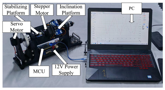
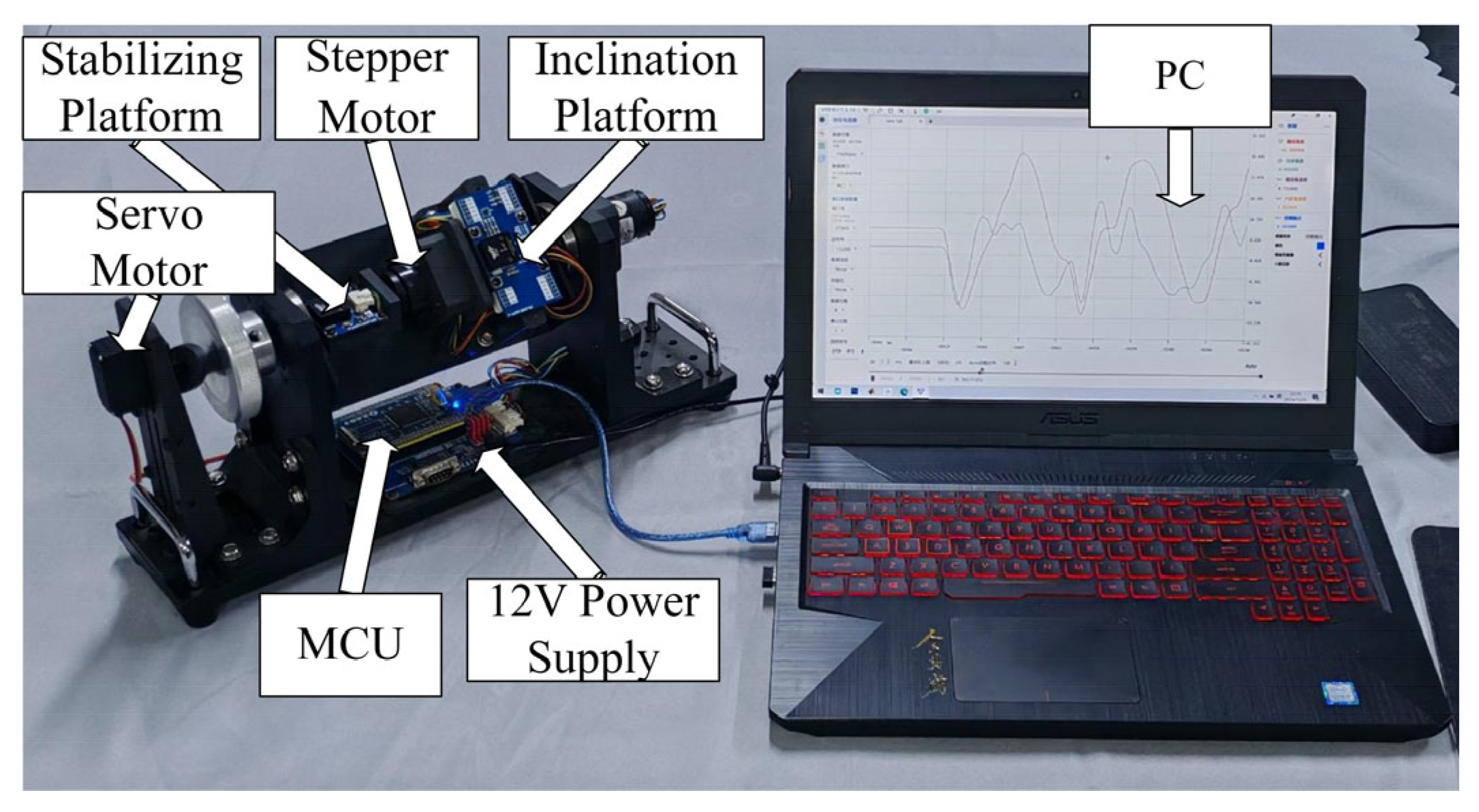
Based on the completion of both hardware and software design, disturbance experiments were conducted to validate the performance of the gimbal system. The disturbance test setup of the gimbal system is shown in Figure 6. During operation, two attitude sensors respectively measure the angular positions of the inclination platform and the stabilizing platform. The measured signals are used as real-time feedback and transmitted to the MCU for processing. All aforementioned components are mounted on the fixed platform. The stepper motor is installed on the inclination platform and rotates together with it. The inclination platform is mechanically coupled with the servo motor horn, while the stabilizing platform is rigidly connected to the output shaft of the stepper motor. All platforms rotate along the same axis. The MCU executes the control algorithm based on the acquired attitude data and sends target position commands to the stepper motor to achieve position control of the stabilizing platform. Finally, experimental data are transmitted to the PC via serial communication for waveform observation and performance evaluation. Disturbances are introduced by oscillating the handle via the servo motor to simulate external interference, while ensuring that the disturbance conditions remain identical across different control strategies for fair comparison. The PSO-tuned parameters listed below are obtained from offline pre-tuning using the simplified surrogate model and are subsequently deployed as initial parameters in the experimental validation. To ensure a fair comparison, the conventional PID controller was tuned using the classical Ziegler–Nichols tuning method to obtain an initial parameter set. The parameters were subsequently fine-tuned within a reasonable range to guarantee closed-loop stability and acceptable transient performance under the same experimental conditions. The tuning objective was to achieve stable operation without excessive overshoot or oscillation, rather than to maximize performance metrics. The parameter settings of the single-neuron adaptive controller and the conventional PID controller are listed in Table 3.
Figure 6.
Disturbance experiment of gimbal.
Table 3.
Controller parameters.
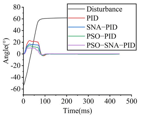
To simulate multi-dimensional disturbance conditions encountered by vehicle-mounted gimbal systems, four verification scenarios are designed: (1) extreme transient impact test; (2) low-frequency and high-frequency disturbance tests; and (3) dynamic reorientation test. The experimental results are analyzed in terms of peak-to-peak value, mean absolute error (MAE), root mean squared error (RMSE), and control effort. The control effort is calculated using the following expression: .
5.1. External Single Large-Amplitude Disturbance of 110°
The servo motor is initialized at −50° and subsequently rotated to 60°, causing the tilting platform to undergo a large-amplitude rotation of 110°. This test is designed to simulate extreme road-induced fluctuations encountered by the gimbal system during vehicle operation. Due to the precision limitations of both the disturbance servo and the gimbal system, the applied disturbance angle exhibits an error of ±1°.
The performance of different control strategies is summarized in Table 4.
Table 4.
Performance indicators under 110° for a large single disturbance.
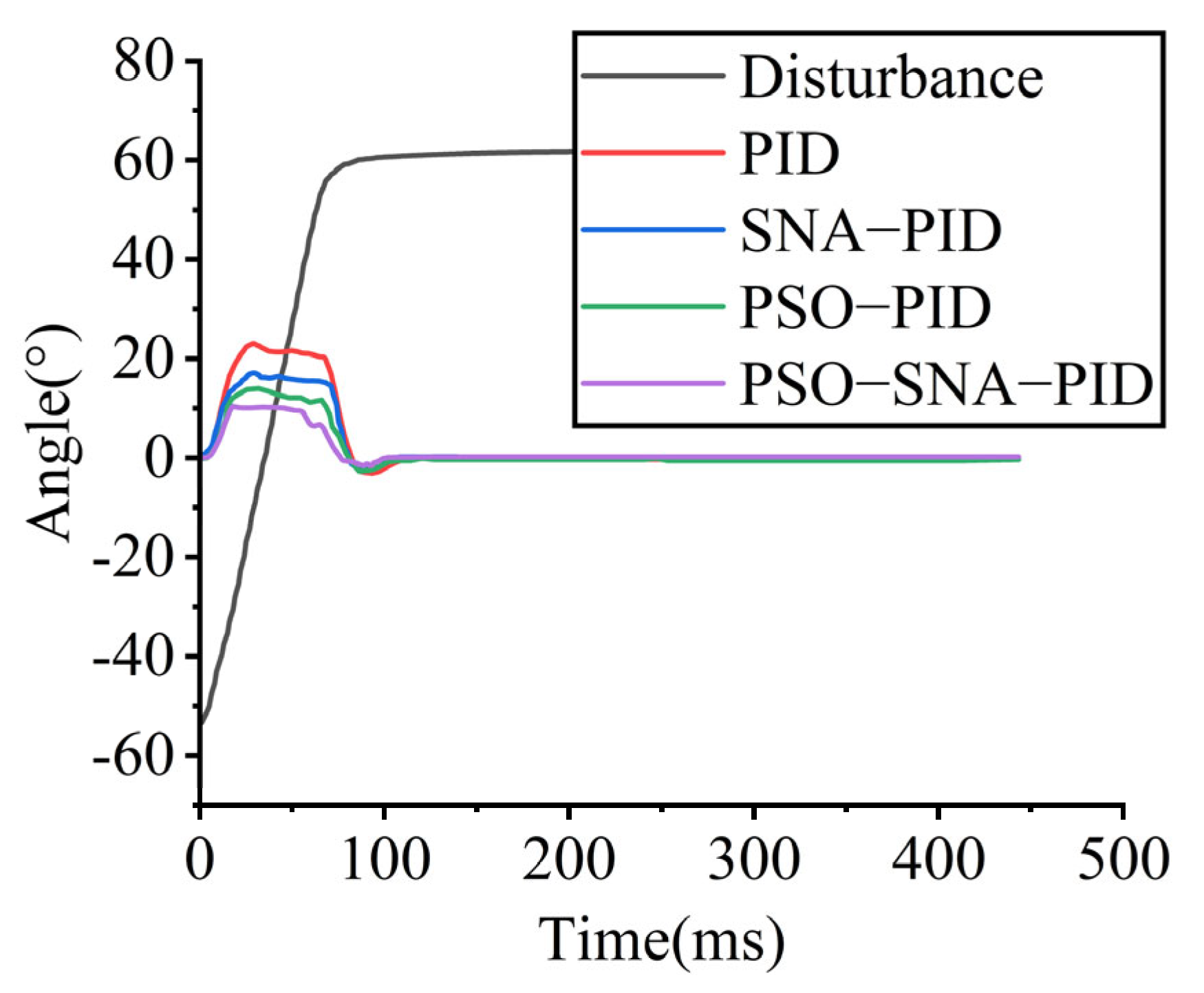
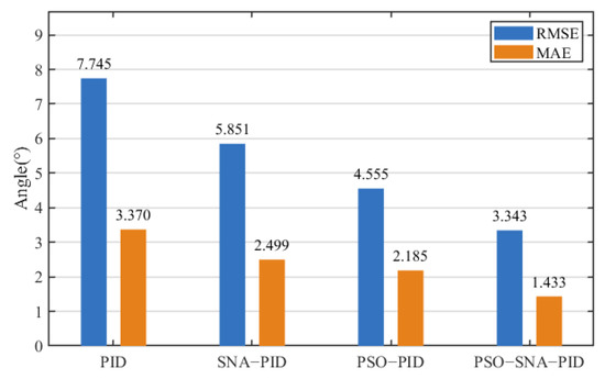
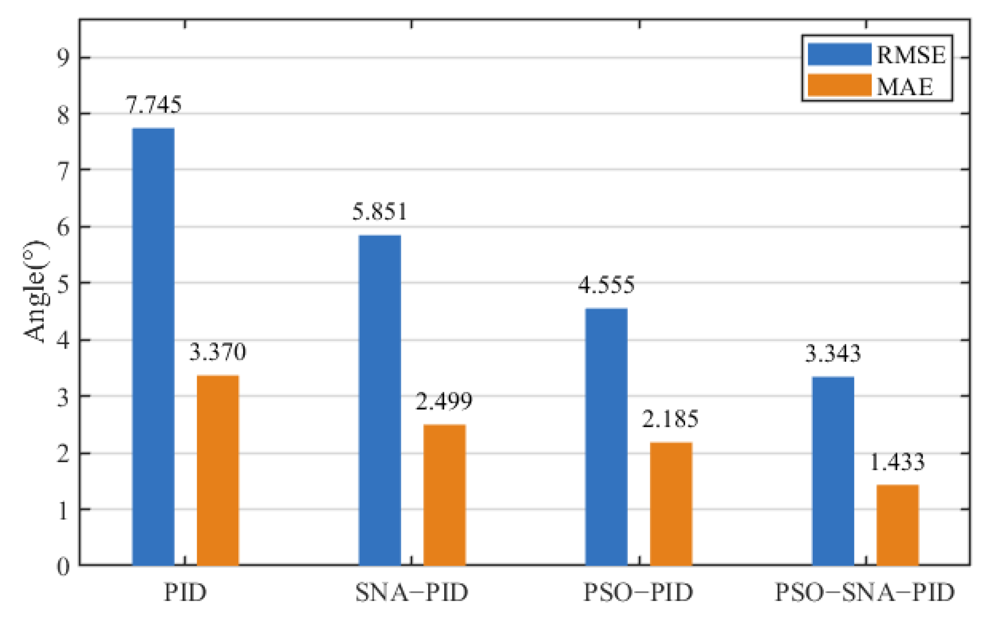
It can be observed that all four control strategies are able to maintain closed-loop stability; however, their control performance differs noticeably. As shown in Figure 7, compared with the PSO−PID, SNA−PID, and conventional PID controllers, the adaptive PID controller based on offline–online cooperative optimization reduces the peak-to-peak value by 28.57%, 37.89%, and 54.25%, respectively. As illustrated in Figure 8, the root mean squared error (RMSE) is reduced by 26.61%, 42.86%, and 56.84%, respectively, while the mean absolute error (MAE) is reduced by 34.42%, 42.66%, and 57.48%, respectively.
Figure 7.
Angle tracking response during the 110° large single disturbance.
Figure 8.
Disturbance error response during the 110° large single disturbance.
In terms of control effort, the conventional PID controller exhibits the highest control effort of 1.492°·s, whereas the adaptive PID controller based on offline–online cooperative optimization achieves the lowest control effort of 0.634°·s. These results indicate that the single-neuron adaptive mechanism can significantly improve control performance through real-time online parameter adjustment. Furthermore, the introduction of the particle swarm optimization algorithm enables global offline search, alleviating sensitivity to initial parameter selection and local optima, thereby effectively reducing angular fluctuations. Since the disturbance is applied in a relatively slow manner, the differences in settling time among the three control strategies are relatively small.
5.2. External 1 Hz Frequency Disturbance
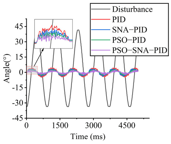
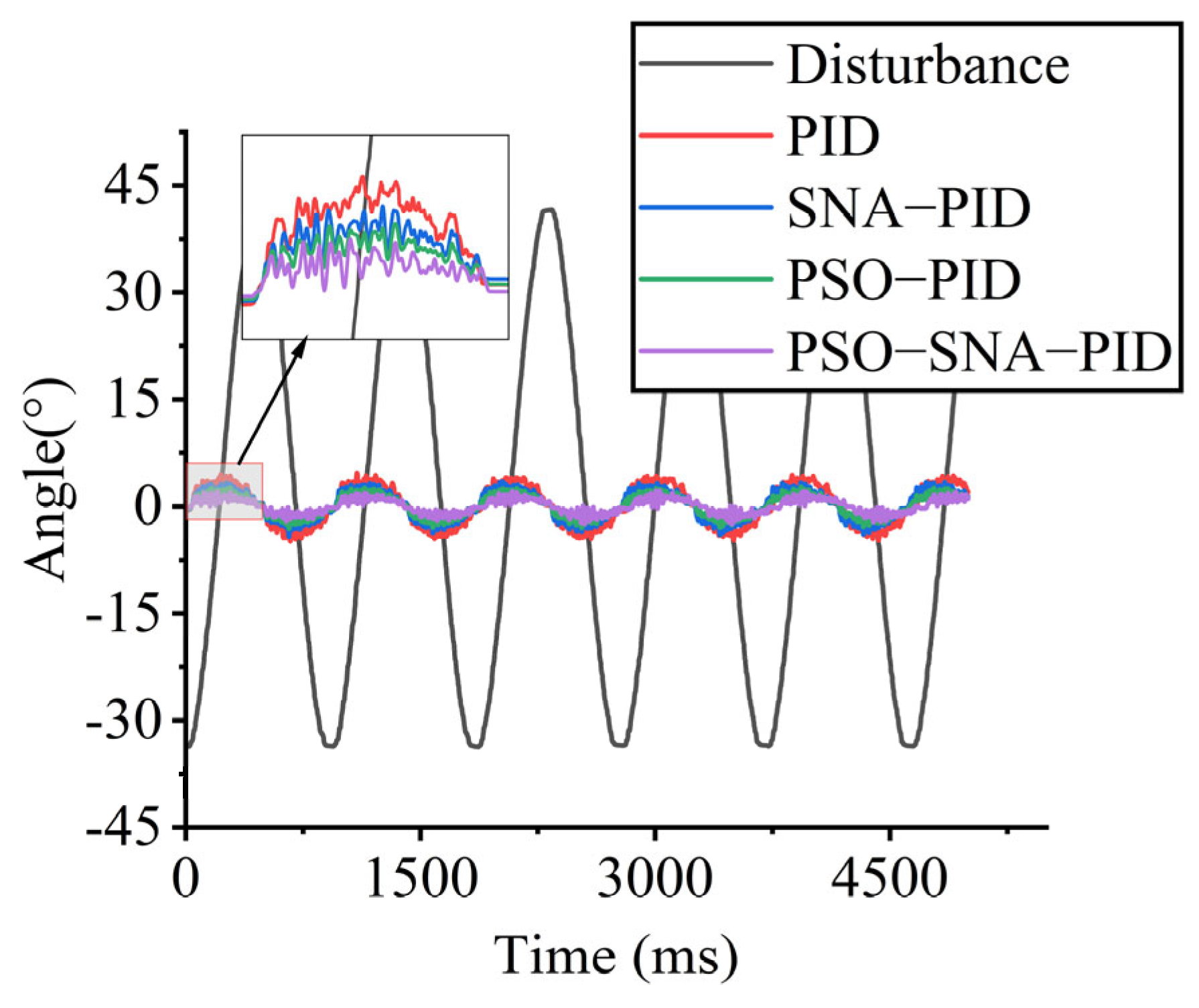
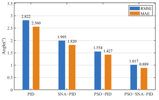
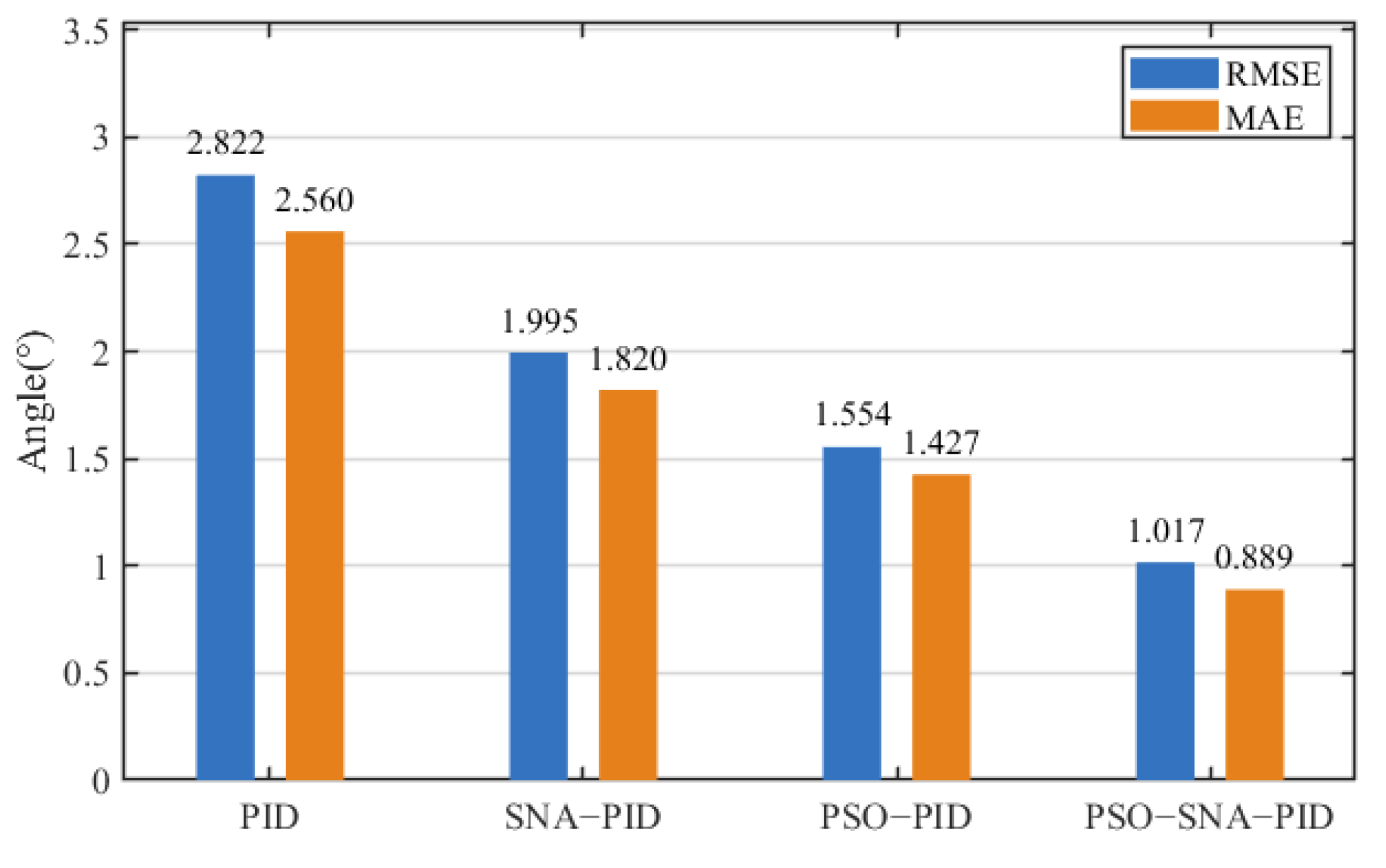
To simulate low-speed driving conditions on uneven road surfaces, the disturbance servo generates a sinusoidal signal with a frequency of 1 Hz, causing the tilting platform to oscillate within an amplitude of 76°. Figure 9 and Figure 10 illustrate the control performance of different control strategies under continuous 1 Hz disturbance conditions.
Figure 9.
Angle tracking response under 1 Hz continuous disturbance.
Figure 10.
Disturbance error response under 1 Hz continuous disturbance.
The quantitative performance indices of each control strategy are summarized in Table 5.
Table 5.
Performance indicators under 1 Hz frequency disturbance.
As shown in Figure 9, compared with the PSO–PID, SNA–PID, and conventional PID controllers, the adaptive PID controller based on offline–online cooperative optimization achieves reductions in the peak-to-peak values of 20.40%, 40.41%, and 51.38%, respectively. As illustrated in Figure 10, the RMSE is reduced by 34.56%, 49.02%, and 63.96%, respectively, while the MAE is reduced by 37.70%, 51.15%, and 65.27%, respectively. In terms of control effort, the conventional PID controller exhibits the highest value of 12.80°·s, whereas the proposed offline–online cooperative adaptive PID controller achieves the lowest control effort of 4.45°·s.
5.3. External 8 Hz Frequency Disturbance
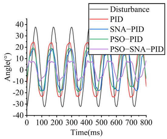
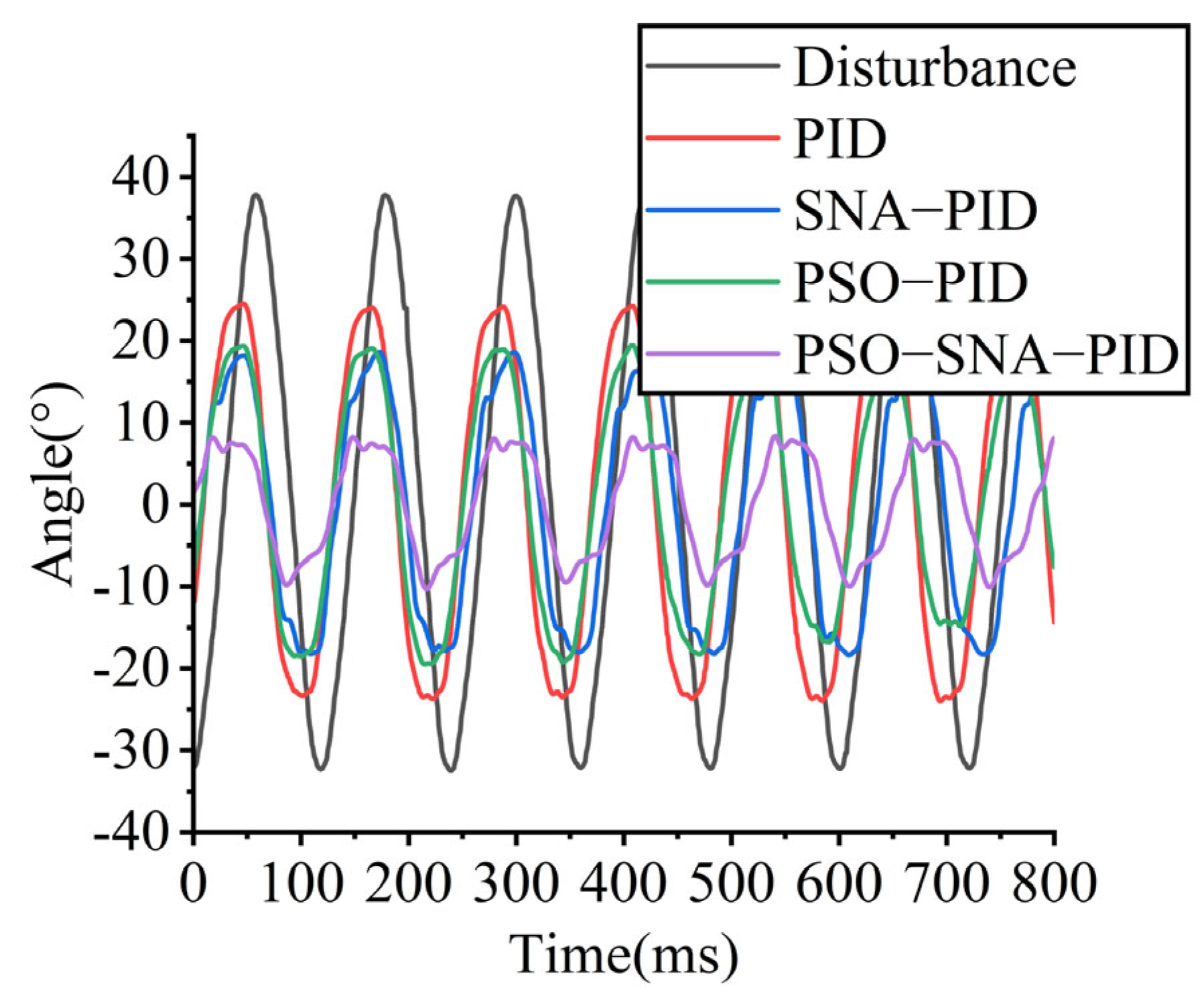
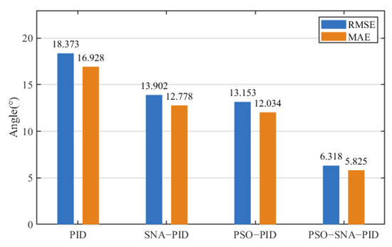
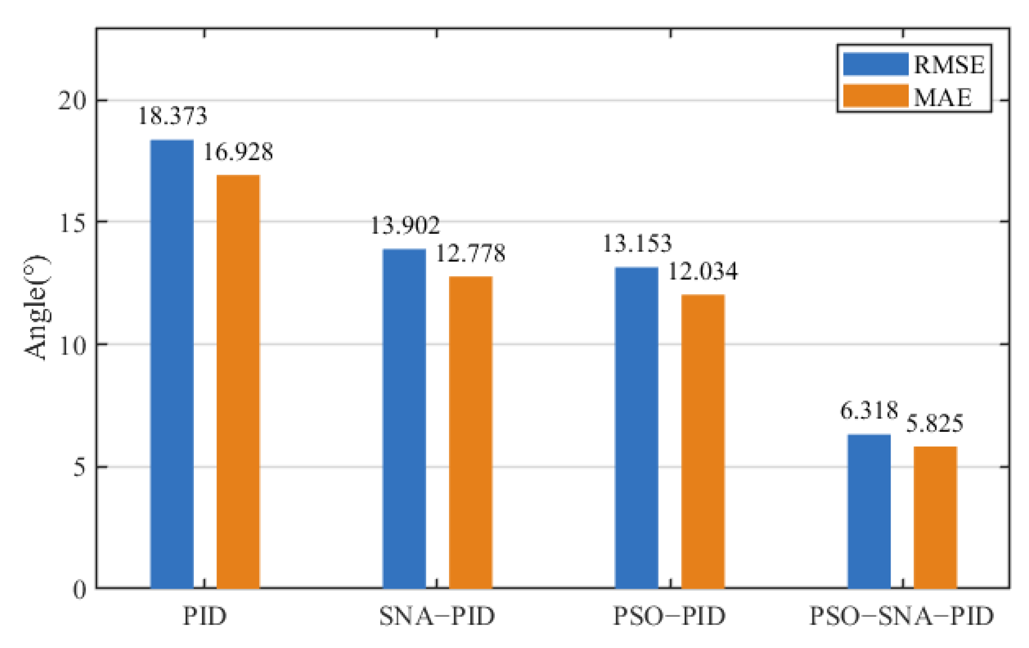
To simulate rapid vehicle motion on highly uneven road surfaces, the disturbance servo generates a sinusoidal signal with a frequency of 8 Hz, causing the tilting platform to oscillate within an amplitude of 70°. Figure 11 and Figure 12 present the control performance under continuous 8 Hz disturbance conditions.
Figure 11.
Angle tracking response under 8 Hz continuous disturbance.
Figure 12.
Disturbance error response under 8 Hz continuous disturbance.
The corresponding performance indices are listed in Table 6.
Table 6.
Performance indicators under 8 Hz frequency disturbance.
As shown in Figure 11, compared with the PSO−PID, SNA−PID, and conventional PID controllers, the adaptive PID controller based on offline–online cooperative optimization reduces the peak-to-peak value by 51.21%, 49.35%, and 60.99%, respectively. As illustrated in Figure 12, the RMSE is reduced by 51.97%, 54.55%, and 65.61%, respectively, while the MAE is reduced by 51.60%, 54.41%, and 65.59%, respectively. In terms of control effort, the conventional PID controller exhibits the highest control effort of 84.642°·s, whereas the proposed controller achieves the lowest value of 29.125°·s. These results indicate that under low-frequency and high-frequency continuous disturbances, the proposed offline–online cooperative adaptive PID controller significantly improves tracking accuracy while simultaneously reducing control effort. The improvement suggests that the combination of offline parameter pre-tuning and online adaptive adjustment effectively enhances disturbance rejection capability in slowly and quickly varying operating conditions.
5.4. Internal Reference Change of 30°
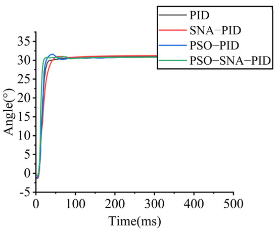
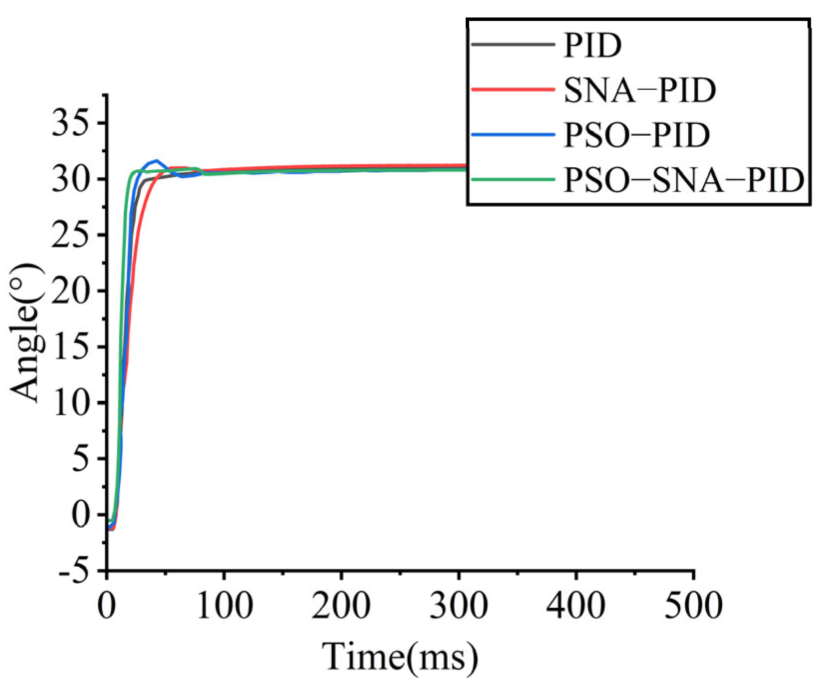
To simulate scenarios in which the gimbal system must rapidly change its target orientation, the control reference is shifted from 0° to 30°, forcing the stabilized platform to rotate quickly toward the new target position.
The performance comparison under internal disturbance is presented in Table 7.
Table 7.
Performance indicators under internal disturbance.
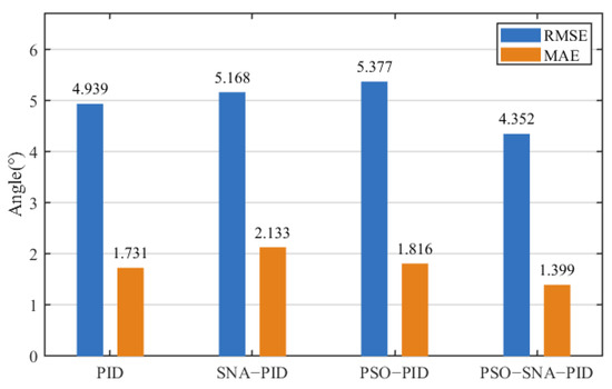
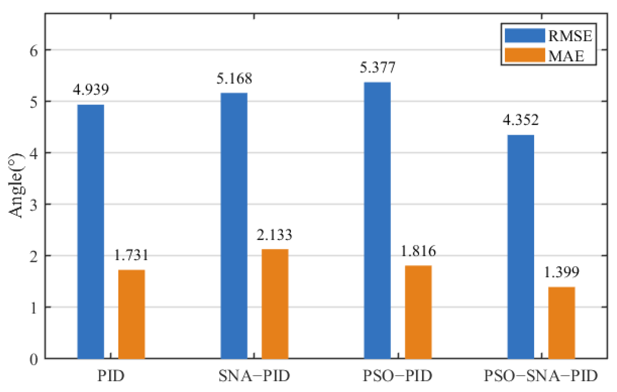
As shown in Figure 13, compared with the PSO−PID, SNA−PID, and conventional PID controllers, the adaptive PID controller based on offline–online cooperative optimization reduces the overshoot by 43.67%, 26.02%, and 4.95%, respectively, and shortens the settling time by 62.96%, 52.38%, and 48.72%, respectively. As illustrated in Figure 14, the RMSE is reduced by 19.06%, 15.79%, and 11.89%, respectively, while the MAE is reduced by 22.96%, 34.41%, and 19.18%, respectively. In terms of control effort, the PSO−PID controller exhibits the highest value of 1.822°·s, whereas the proposed controller achieves the lowest control effort of 0.726°·s. These results demonstrate that the offline–online cooperative adaptive PID controller achieves faster response and improved tracking accuracy during internal reference changes. The combined effect of single-neuron adaptation and optimized initial parameters effectively enhances transient performance while maintaining low control effort.
Figure 13.
Angle tracking response under internal disturbance.
Figure 14.
Error response under internal disturbance.
6. Conclusions
This study proposes an adaptive PID control strategy based on an offline–online cooperative framework to improve response speed, stability, and disturbance rejection in gimbal stabilization. The offline stage provides reasonable initial parameters through optimization on a simplified surrogate model, while a single-neuron adaptive mechanism performs real-time parameter adjustment during operation to compensate for aggregated disturbances and operating variations. Experimental results on the physical gimbal platform demonstrate that, under reference changes and external disturbances, the proposed strategy reduces angular fluctuations and shortens settling time while maintaining smooth control behavior. Compared with conventional fixed-parameter control, the cooperative approach achieves improved comprehensive performance within the tested scenarios. The framework remains lightweight and suitable for implementation on resource-constrained embedded platforms, reducing parameter tuning effort and enhancing operational reliability. Nevertheless, the present validation is limited to a single-axis system, and offline pre-tuning relies on a simplified linear surrogate model. Although the online adaptive mechanism mitigates modeling inaccuracies during operation, further investigation under strongly coupled multi-axis conditions would provide deeper insight. In addition, a systematic benchmarking study against more advanced modern control strategies was not conducted in this work. Future research will focus on multi-axis coordinated control, refined modeling, and broader comparative evaluations to further assess performance–complexity trade-offs.
Author Contributions
Conceptualization, J.Y.; methodology, J.L.; software, M.C.; validation, J.L., H.Z. and J.Y.; formal analysis, H.Z.; investigation, Y.Y.; resources, J.Y. and Y.Y.; data curation, J.L.; writing—original draft preparation, J.L.; writing—review and editing, J.Y.; visualization, M.C.; supervision, Y.Y.; project administration, M.C.; funding acquisition, J.Y. All authors have read and agreed to the published version of the manuscript.
Funding
This research was funded by the 2025 Guangxi Key Research and Development Program —“Empowerment” Action Plan, the 2023 Guilin Key Research and Development Project, and the 2025 Guangxi Science and Technology Plan Project—Central Guidance Fund for Local Science and Technology Development, grant number GUIKEFN2504240015, 20231B04737523 and 2025XTXTO1017.
Data Availability Statement
Data are contained within the article.
Conflicts of Interest
The authors declare no conflicts of interest. The funders had no role in the design of the study; in the collection, analyses, or interpretation of data; in the writing of the manuscript; or in the decision to publish the results.
References
- Moysiadis, V.; Tsolakis, N.; Katikaridis, D.; Sørensen, C.G.; Pearson, S.; Bochtis, D. Mobile Robotics in Agricultural Operations: A Narrative Review on Planning Aspects. Appl. Sci. 2020, 10, 3453. [Google Scholar] [CrossRef] [Scilit]
- Shen, C.; Chen, N.; Tan, R.; Fan, S.; Fan, D. Modeling and Stability Analysis of Coarse-Fine Composite Mechatronic System in UAV Multi-Gimbal Electro-Optical Pod. Electronics 2020, 9, 769. [Google Scholar] [CrossRef] [Scilit]
- Hussain, M.; He, L.; Schupp, J.; Lyons, D.; Heinemann, P. Green fruit segmentation and orientation estimation for robotic green fruit thinning of apples. Comput. Electron. Agric. 2023, 207, 107734. [Google Scholar] [CrossRef] [Scilit]
- Fasiolo, D.T.; Pichierri, A.; Sivilotti, P.; Scalera, L. An analysis of the effects of water regime on grapevine canopy status using a UAV and a mobile robot. Smart Agric. Technol. 2023, 6, 100344. [Google Scholar] [CrossRef] [Scilit]
- Rumson, A.G. The application of fully unmanned robotic systems for inspection of subsea pipelines. Ocean Eng. 2021, 235, 109214. [Google Scholar] [CrossRef] [Scilit]
- Liaw, S.H.; Lee, T.C. A Brief Review of Artificial Intelligence Robotic in Food Industry. Procedia Comput. Sci. 2024, 232, 1694–1700. [Google Scholar] [CrossRef] [Scilit]
- Ma, W.; Wang, X.; Yang, S.X.; Xue, X.; Li, M.; Wang, R.; Yu, L.; Song, L.; Li, Q. Autonomous inspection robot for dead laying hens in caged layer house. Comput. Electron. Agric. 2024, 227, 109595. [Google Scholar] [CrossRef] [Scilit]
- Yu, R.D.; Man, L.; Jiu, X.W.; Xin, R.L.; Kai, H.W.; Zi, S.L.; Qi, D.; Jia, H.Y.; Ding, Z.L.; Yao, H.S. A wall climbing robot based on machine vision for automatic welding seam inspection. Ocean Eng. 2024, 310, 118825. [Google Scholar] [CrossRef] [Scilit]
- Qian, W.D.; Xi, Z.; Qiu, N.H.; Xing, L.C.; Wan, S.L.; Yao, M. Pointing control design based on the PID type-III control loop for two-axis gimbal systems. Sens. Actuators A Phys. 2021, 331, 112923. [Google Scholar] [CrossRef] [Scilit]
- Altan, A.; Hacioglu, R. Model predictive control of three-axis gimbal system mounted on UAV for real-time target tracking under external disturbances. Mech. Syst. Signal Process. 2020, 138, 106548. [Google Scholar] [CrossRef] [Scilit]
- Königseder, F.; Kemmetmüller, W.; Kugi, A. Attitude control strategy for a camera stabilization platform. Mechatronics 2017, 46, 60–69. [Google Scholar] [CrossRef] [Scilit]
- Liu, G.P.; Daley, S. Optimal-tuning PID control for industrial systems. Control Eng. Pract. 2001, 9, 1185–1194. [Google Scholar] [CrossRef] [Scilit]
- Meng, M.J.; Long, W.; Yong, B.L.; Wen, C.Z. Study on Fuzzy PID control with an improved genetic algorithm for boiler drum water level. Eng. Res. Express 2025, 7, 45320. [Google Scholar] [CrossRef] [Scilit]
- Lu, H.Y.; Jin, G.S.; Liu, L.Z. Research on Servo Control Strategy of Opto-electronic Tracking Turntable. Laser Infrared 2018, 48, 503–508. [Google Scholar]
- Abro, G.E.M.; Bin, M.Z.S.A.; Asirvadam, V.S. Dual-loop single dimension fuzzy-based sliding mode control design for robust tracking of an underactuated quadrotor craft. Asian J. Control 2023, 25, 144–169. [Google Scholar] [CrossRef] [Scilit]
- Ali, M.H.; Anwar, M.N. Sliding mode controller design for unstable processes with dead time with a case study on continuous stirred tank reactor. Eng. Res. Express 2023, 5, 045044. [Google Scholar] [CrossRef] [Scilit]
- Han, J.Q. Auto Disturbances Rejection Control Technique. Front. Sci. 2007, 1, 24–31. [Google Scholar]
- Han, J.Q. From PID Technique to Active Disturbances Rejection Control Technique. Control Eng. China 2002, 9, 13–18. [Google Scholar]
- Yuan, B.; Li, H.; Xiang, X.; Zhou, T. Precision Position Servo PMSM Fast-Response Control Based on Trajectory Planning and ADRC. Electronics 2025, 14, 2062. [Google Scholar] [CrossRef] [Scilit]
- Zhi, Q.G. Scaling and bandwidth-parameterization based controller tuning. In Proceedings of the 2003 American Control Conference, Denver, CO, USA, 4–6 June 2003; Volume 6, pp. 4989–4996. [Google Scholar] [CrossRef] [Scilit]
- Tan, W.; Fu, C.F. Linear active disturbance-rejection control: Analysis and tuning via IMC. IEEE Trans. Ind. Electron. 2016, 63, 2350–2359. [Google Scholar] [CrossRef] [Scilit]
- Han, J.Q. Active Disturbance Rejection Control Technique the Technique for Estimating and Compensating the Uncertainties; National Defense Industry Press: Beijing, China, 2008; pp. 282–283. [Google Scholar]
- Dai, Y. Research on Intelligent PID Control Method for Manipulator. Master’s Thesis, Shenyang Ligong University, Shenyang, China, 2016. [Google Scholar]
- Wang, Y.Y. Research on Control Method of Hypersonic Vehicle with Large Time Delay System Based on Neural Network. Master’s Thesis, National University of Defense Technology, Changsha, China, 2017. [Google Scholar]
- Liu, H.; Wang, R.; Sun, F.; Xing, X. Adaptive self-structuring neural network control for full-state constrained hydraulic systems with disturbance compensation. Appl. Math. Model. 2024, 129, 1–24. [Google Scholar] [CrossRef] [Scilit]
- Li, Z.; Dai, Y.; Tang, P. Adaptive Neural Network Control with Fuzzy Compensation for Upper Limb Exoskeleton in Active Spacesuit. Electronics 2021, 10, 638. [Google Scholar] [CrossRef] [Scilit]
- Hernandez-Barragan, J.; Rios, J.D.; Alanis, A.Y.; Lopez-Franco, C.; Gomez-Avila, J.; Arana-Daniel, N. Adaptive Single Neuron Anti-Windup PID Controller Based on the Extended Kalman Filter Algorithm. Electronics 2020, 9, 636. [Google Scholar] [CrossRef] [Scilit]
- Cao, Q.; Hong, Y.; Zhou, J.; Wang, H. Vibration control of flexible manipulator based on self-tuning PID controller by PSO. J. Vib. Meas. Diagn. 2014, 34, 1045–1049. [Google Scholar]
- Xin, L.G.; Yan, L.; Chen, X.G.; Jian, Q.M. Research on wavefront correction based on single neuron PID controller. Laser Infrared 2025, 8, 1272–1278. [Google Scholar]
- Qin, Y.; Duan, H. Single-Neuron Adaptive Hysteresis Compensation of Piezoelectric Actuator Based on Hebb Learning Rules. Micromachines 2020, 11, 84. [Google Scholar] [CrossRef] [Scilit]
- Sahu, P.; Dey, R. An improved 2-level MPPT scheme for photovoltaic systems using a novel high-frequency learning based adjustable gain-MRAC controller. Sci. Rep. 2021, 11, 23131. [Google Scholar] [CrossRef] [Scilit]

Disclaimer/Publisher’s Note: The statements, opinions and data contained in all publications are solely those of the individual author(s) and contributor(s) and not of MDPI and/or the editor(s). MDPI and/or the editor(s) disclaim responsibility for any injury to people or property resulting from any ideas, methods, instructions or products referred to in the content. |
© 2026 by the authors. Licensee MDPI, Basel, Switzerland. This article is an open access article distributed under the terms and conditions of the Creative Commons Attribution (CC BY) license.