Distribution Network Partitioning Method Based on Integrated Electrical Distance and Improved DPC-LPA

Abstract

Distribution network partitioning at high distributed-energy-resource penetration is challenged by operating-point-insensitive distance criteria, initialization dependence, and oversized or oscillatory zones. This paper presents a framework that combines a comprehensive electrical distance metric with an improved density peak clustering–label propagation algorithm (DPC-LPA). The metric integrates network impedance and voltage sensitivities to renewable-power variations. DPC determines the initial number and centers of zones, and the modified LPA uses partition-scale, load-balance, and historical-influence factors to regulate zone growth and label switching. Tests on medium- and low-voltage alternating-current/direct-current (AC/DC) networks show improved load balance relative to conventional LPA with only a modest change in modularity. These results support the method for the evaluated networks without implying performance beyond the tested conditions.

1. Introduction

The distribution network directly connects the power system to end users. As distributed generation displaces the one-way power-flow pattern of conventional radial feeders, variable renewable injections increase the difficulty of maintaining voltage quality, stability, and coordinated control [1]. Partitioning the network into electrically coherent zones can reduce model and control complexity, facilitate short-circuit current management, and improve operational reliability [2].

Energy storage can absorb renewable surpluses and supply deficits, thereby reducing net-load ramps and supporting voltage and power balance. For battery energy storage systems (BESSs), coordinated charging, distributed power allocation, state-of-charge (SoC) balancing, and discharge-rate constraints affect usable capacity and microgrid stability under time-varying demand and intermittent communication [3,4]. Storage dispatch is not optimized in this study, but the resulting zones can provide units for subsequent source–load–storage coordination.

These benefits depend on whether the partition reflects the actual operating condition. Under high distributed generation penetration, a distance based only on a fixed network structure may overlook changes in voltage coupling caused by renewable injections. Reproducibility is further affected when the number and centers of zones are chosen subjectively, and unconstrained label propagation may yield oversized zones or oscillating assignments.

Previous studies have mainly improved either the distance criterion or the solution procedure. Reference [5] combined an electrical distance modularity index with generation–load–storage matching. References [6,7] derived voltage-sensitivity matrices; [8] refined PV active/reactive-power–voltage sensitivity; [9] introduced PV uncertainty into an expected electrical distance metric; [10] examined branch reactive-power–voltage sensitivity and propagation paths; and [11] developed indicators for high-renewable networks. Taken individually, however, these formulations do not jointly represent multi-source voltage coupling and network-structural separation.

The cited formulations retain complementary information. The impedance-based modularity formulation in [5] describes structural location but responds weakly to the operating point. Node- and branch-voltage-sensitivity formulations [6,7,8,10] represent active- or reactive-power/voltage response without retaining the complete impedance path. The expected-distance formulation in [9] incorporates renewable uncertainty but does not combine multi-source active/reactive coupling and structural separation in one pairwise metric. The proposed formulation addresses this representational gap by coupling the resistance/active-power and reactance/reactive-power channels; it is not assumed to dominate all distance definitions under all operating conditions.

Algorithmic studies have used clustering, optimization, and community-detection methods [12]. The Girvan–Newman framework provides the modularity basis for evaluating community structure [13,14]. Label propagation is attractive because of its low computational cost, but its outcome depends on the initial labels; it may also generate oversized communities and cannot determine the number or centers of zones independently.

Recent distribution network studies [5,6,7,8,9,10,11,12] have emphasized application-specific electrical distance, voltage sensitivity, renewable uncertainty, and clustering indicators, whereas the broader network-science literature [13,14] established general community structure and modularity frameworks. The unresolved problem is a unified workflow that represents renewable-dependent coupling, initializes the number and centers of zones objectively, and controls size/load imbalance and label oscillation.

To address this combined metric-and-initialization problem, the study links scenario construction, electrical distance calculation, and two-stage clustering in one workflow. Section 2 defines the representative renewable operating point, Section 3 constructs the distance metric, and Section 4 combines DPC initialization with LPA refinement. Section 5 evaluates the method on medium- and low-voltage AC/DC networks.

Compared with methods that prespecify partition centers or use network topology alone, the framework incorporates renewable-output scenarios into electrical distance, determines the number and centers of zones through DPC, and uses the modified LPA to limit oversized zones and label oscillation. The graph-based workflow is applicable across the voltage levels evaluated here and reduces sensitivity to initialization while improving zone size and load balance.

The resulting zones are intended as engineering coordination units rather than simply smaller graph communities. Grouping nodes with similar electrical responses while constraining size and load imbalance can support local voltage/reactive-power coordination, source–load balance, and distributed-energy management. The study therefore addresses three problems: operating-point-insensitive distance, subjective initialization, and unstable or unbalanced label propagation. Only the partitioning layer is evaluated; downstream control and economic effects are outside the present scope.

2. Generation of Typical Scenarios for Distributed Power Sources

Wind speed and solar irradiance are the primary meteorological drivers of wind and PV output, respectively. This section fits a probability distribution to each variable and selects one high-probability representative value. The resulting wind- and PV-power values define the common operating point used to construct the electrical distance matrix.

2.1. Wind Speed Distribution and Wind Farm Output Model Based on Weibull Distribution

Wind turbine output is uncertain because wind speed is intermittent and variable. A two-parameter Weibull distribution is widely used to represent wind speed frequency, and a piecewise power curve maps wind speed to wind turbine output through the cut-in, rated, and cut-out speeds [15,16]. The probability density function (PDF) and cumulative distribution function (CDF) are expressed as Equations (1) and (2), respectively.

$$f_w(v;c,k)=\left({\displaystyle \frac{k}{c}}\right){\left({\displaystyle \frac{v}{c}}\right)}^{k-1}\exp \left[-{\left({\displaystyle \frac{v}{c}}\right)}^k\right],$$

(1)

$$F_w(v;c,k)=1-\exp [-{(v/c)}^k],$$

(2)

where $F_w(v,c,k)$ is the distribution function of the two-parameter Weibull distribution, $c$ is the scale parameter of the Weibull distribution, $v$ is the actual wind speed, and $k$ is the shape parameter of the Weibull distribution.

For a wind speed sample $v=\left\{v_1,v_2,\cdots ,v_n\right\}$, maximum-likelihood estimation selects the Weibull shape and scale parameters that maximize the product of the sample probability densities. The equivalent log-likelihood is

$$\log L(c,k;V)={\displaystyle \sum _{i=1}^n}\left[\log \left({\displaystyle \frac{k}{c}}\right)+(k-1)\log \left({\displaystyle \frac{v_i}{c}}\right)-{\left({\displaystyle \frac{v_i}{c}}\right)}^k\right].$$

(3)

The scale and shape parameters are obtained by numerically maximizing the log-likelihood function. The output power of a wind turbine is then represented by the piecewise function in Equation (4).

$$P_w(v)=\left\{\begin{array}{cc}0\hfill & \hfill v\le v_{ci},v>v_{co}\\ P_r{\displaystyle \frac{v-v_{ci}}{v_r-v_{ci}}}\hfill & \hfill v_{ci}\le v\le v_r\\ P_r\hfill & \hfill v_r\le v\le v_{co}\end{array}\right.,$$

(4)

In the formula,$v_{ci}$ represents the cut-in wind speed of the wind turbine, $v_r$ denotes the rated wind speed, $v_{co}$ indicates the cut-out wind speed, and $P_r$ signifies the rated output power.

Equation (4) is a steady-state planning model with cut-in, rated, and cut-out regions and a rated-power ceiling. It excludes ramp-rate limits, wake effects, availability, curtailment, and electromechanical transients and is used only to define the renewable-injection operating point for partitioning.

2.2. Beta-Distributed Solar Irradiance and PV-Power Model

PV-power uncertainty is primarily driven by solar irradiance variability. Because normalized irradiance is bounded on [0, 1], the Beta distribution provides a suitable probabilistic representation and has been used in PV-output and irradiance-forecasting studies [15,17,18]. Its PDF is given by Equation (5).

$$f(s;\alpha ,\beta )={\displaystyle \frac{\Gamma (\alpha +\beta )}{\Gamma (\alpha )\Gamma (\beta )}}{s}^{\left(\alpha -1\right)}{(1-s)}^{\left(\beta -1\right)},$$

(5)

where $\Gamma (·)$ denotes the gamma function, $s$ represents local solar irradiance, $f(s;\alpha ,\beta )$ is the probability density function for solar irradiance $s$, and $\alpha$ and $\beta$ are the shape parameters of the Beta distribution.

The mean and variance of the Beta distribution are given by Equations (6) and (7), respectively.

$$\mu ={\displaystyle \frac{\alpha }{\alpha +\beta }};$$

(6)

$${\sigma }^2={\displaystyle \frac{\alpha \beta }{(\alpha +\beta +1){(\alpha +\beta )}^2}}.$$

(7)

Let $\mu =\mathbb{E}[s]$ and ${\sigma }^2=\mathrm{Var}(s)$ denote the sample mean and sample variance, respectively, of the normalized solar irradiance $s$. Provided that $0<\mu <1$ and $0<{\sigma }^2<\mu (1-\mu )$, the positive Beta shape parameters $\alpha$ and $\beta$ are estimated separately from the historical observations using Equations (8) and (9), respectively.

$$\alpha =\mu \left[{\displaystyle \frac{\mu (1-\mu )}{{\sigma }^2}}-1\right];$$

(8)

$$\beta =(1-\mu )\left[{\displaystyle \frac{\mu (1-\mu )}{{\sigma }^2}}-1\right].$$

(9)

The PV generator output is approximated as a function of solar irradiance using Equation (10).

$$P_a=\left\{\begin{array}{cc}s{P}_{a,\max }& s\le s_e\\ P_{a,\max }& s>s_e\end{array}\right.,$$

(10)

where $P_{a,\max }$ denotes the rated power of the PV generator set, and $s_e$ represents the rated solar irradiance.

Equation (10) is also a screening-level steady-state mapping. It excludes module-temperature dependence, nonlinear inverter efficiency, clipping, shading, curtailment, and long-term degradation. Operational studies should calculate node-specific AC output with a temperature-aware module model and the applicable inverter-efficiency curve before reconstructing the electrical distance matrix.

2.3. Probabilistic Scenario-Selection Method for Distributed Generation Output

To obtain a tractable operating point for partitioning, the historical wind speed and solar irradiance records are fitted with the models in Section 2.1 and Section 2.2, respectively. One representative value is then selected for each resource from a high-probability interval [19].

After data preprocessing, the Weibull parameters are estimated from the wind speed sample and the Beta parameters from the normalized irradiance sample.

For each fitted distribution, the range is divided into consecutive intervals and the probability mass of each interval is calculated. The interval with the largest mass is treated as the most frequently occurring range in the available record.

Its midpoint is used as the representative value unless an engineering constraint supports another value. The corresponding source outputs are then used in the power-flow and electrical distance calculations.

This reduction does not preserve the annual mean, variance, tail behavior, wind–solar dependence, or ramp chronology. Annual Weibull and Beta fits also assume marginal stationarity and omit autocorrelation and seasonal regimes. The selected values therefore represent a planning snapshot rather than a stochastic equivalent of the full time series.

A multi-scenario assessment should compare the selected outputs with sample means and quantiles, recompute distance matrices for seasonal or probability-weighted scenarios, and report matrix deviations and label changes. Such analysis is reserved for future work; the present results apply only to the dominant representative scenario.

For an alternative operating point, the renewable outputs, power-flow solution, voltage-sensitivity matrices, and comprehensive electrical distance matrix must be recomputed before rerunning DPC-LPA.

Planning studies with pronounced variability should evaluate several scenarios, either by deriving a consensus partition from scenario-specific labels or by clustering a probability-weighted distance matrix. The present case study does not establish invariant partitions under source–load fluctuations.

3. Comprehensive Metric Considering Node Location and Distributed-Source Output

Distributed-source injections change the operating point and hence the voltage coupling among nodes; this effect becomes more pronounced as penetration increases. An impedance-only metric represents the network structure but not the injection-dependent response. The metric developed below combines both components to define the edge weights for partitioning.

3.1. Electrical Distance Metric Based on Node Location

In power systems, electrical distance represents the electrical coupling relationship between two nodes [19]. When considering only the spatial position of nodes within the distribution network, the electrical distance between node $i$ and node $j$ is commonly expressed using impedance, which can be represented as

$$Z_{ij,\mathrm{equ}}=U_{ij}/I_{ij},$$

(11)

In the equation, $U_{ij}$ and $I_{ij}$ represent the voltage and current between node $i$ and node $j$, respectively.

The impedance $Z_{ij,\mathrm{equ}}$ can be expressed according to the literature [20] as

$$Z_{ij,\mathrm{equ}}=\left(Z_{ii}-Z_{ij}\right)-\left(Z_{ji}-Z_{jj}\right),$$

(12)

where $Z_{ij}$ denotes the element in the $i^{th}$ row and $j^{th}$ column of the distribution network node impedance matrix.

Although this impedance-based quantity describes structural separation, it cannot reflect the voltage response to changes in active- and reactive-power injections. Section 3.2 therefore augments it with voltage-sensitivity information.

3.2. Comprehensive Electrical Distance Considering Node Location and Distributed Generation Output

The Newton–Raphson power-flow equations linearize the coupling among nodal electrical variables through the Jacobian matrix:

$$\left[\begin{array}{c}\Delta P\hfill \\ \Delta Q\hfill \end{array}\right]=\left[\begin{array}{cc}{\displaystyle \frac{\partial P}{\partial \theta }}& {\displaystyle \frac{\partial P}{\partial U}}\\ {\displaystyle \frac{\partial Q}{\partial \theta }}& {\displaystyle \frac{\partial Q}{\partial U}}\end{array}\right]\left[\begin{array}{l}\Delta \theta \hfill \\ \Delta U\hfill \end{array}\right]=\left[\begin{array}{cc}{A}_{P\theta }& B_{PV}\\ C_{Q\theta }& D_{QV}\end{array}\right]\left[\begin{array}{l}\Delta \theta \hfill \\ \Delta U\hfill \end{array}\right],$$

(13)

where $A_{P\theta }$, $B_{PV}$, $C_{Q\theta }$, and $D_{QV}$ denote the Jacobian matrices for corresponding variables in AC and DC distribution networks. Inverting the Jacobian matrix yields sensitivity matrices of different types.

At a converged steady-state operating point, the AC-state, DC-state, and active converter-control derivatives are assembled into a single coupled Jacobian. Slack and directly controlled states are removed before solving the reduced linear systems for the voltage-sensitivity blocks; isolated AC and DC submatrices are not inverted separately. This procedure requires a nonsingular, adequately conditioned reduced Jacobian. Topology or converter-control changes require recalculation of the power flow, Jacobian, and sensitivities; converter inner-loop dynamics are outside the model.

$$\left[\begin{array}{l}\Delta \theta \hfill \\ \Delta U\hfill \end{array}\right]=\left[\begin{array}{cc}{S}_{P\theta }& S_{Q\theta }\\ S_{PU}& S_{QU}\end{array}\right]\left[\begin{array}{l}\Delta P\hfill \\ \Delta Q\hfill \end{array}\right].$$

(14)

Here, the sensitivity matrix $S_{P\theta }$ represents the influence of the node’s injected active-power change $\Delta P$ on the node’s phase angle change $\Delta \theta$, while the sensitivity matrix $S_{Q\theta }$ represents the influence of the node’s injected reactive-power change $\Delta Q$ on the node’s phase angle change $\Delta \theta$. The sensitivity matrix $S_{PU}$ represents the influence of the node’s injected active-power change $\Delta P$ on the node’s voltage change $\Delta U$, while the sensitivity matrix $S_{QU}$ represents the influence of the node’s injected reactive-power change $\Delta Q$ on the node’s voltage change $\Delta U$.

The voltage-sensitivity matrices $S_{PU}$ and $S_{QU}$ quantify the changes in voltage magnitude produced by active- and reactive-power injections, respectively. The voltage change at any node is therefore expressed as a linear combination of injections throughout the network:

$$\Delta U=S_{PU}\cdot \Delta P+S_{QU}\cdot \Delta Q,$$

(15)

where $\Delta P$ and $\Delta Q$ represent the matrix form of power changes across all network nodes, i.e., $\Delta P=\left[\Delta P_1,\Delta P_2,\cdots ,\Delta P_N\right]$ $\Delta Q=\left[\Delta Q_1,\Delta Q_2,\cdots ,\Delta Q_N\right]$.

Equation (15) shows that a node-voltage change depends not only on the local injection but also on power changes at other nodes, particularly those connected to variable distributed sources.

Accordingly, the voltage-sensitive electrical distances $e_{ij}^{QU}$ and $e_{ij}^{\mathrm{PU}}$ are defined for voltage changes induced by distributed-resource injections:

$$e_{ij}^{QU}=S_{QU}^{ii}+S_{QU}^{jj}-S_{QU}^{ij}-S_{QU}^{ji};$$

(16)

$$e_{ij}^{\mathrm{PU}}=S_{PU}^{\ddot{ii}}+S_{PU}^{jj}-S_{PU}^{ij}-S_{PU}^{ji}.$$

(17)

To represent both network location and injection-dependent response, the electrical distances $Z_{ij,\mathrm{equ}}$, $e_{ij}^{QU}$, and $e_{ij}^{\mathrm{PU}}$ are combined.

Therefore, the redefined comprehensive electrical distance $e(i,j)$ can be expressed as

$$e(i,j)=\mathrm{Re}\left(Z_{ij,\mathrm{equ}}\right)e_{ij}^{\mathrm{PU}}+Im\left(Z_{ij,\mathrm{equ}}\right)e_{ij}^{\mathrm{QU}}.$$

(18)

The weighted graph produced by Equation (18) contains both structural and operating-state information and is used directly by DPC-LPA. Its physical interpretation is given below, and its geographical and operational limitations are discussed in Section 5.3.

Equation (18) couples two physically distinct channels. The resistance term reflects the path relevant to active-power transfer, and the active-power sensitivity distance measures differential voltage response to active injections. Their product is large when a node pair is separated both structurally and in active-power response. The reactance/reactive-power term has the analogous interpretation. Their sum provides a single relative dissimilarity for clustering after per-unit normalization.

No additional empirical scalar weight is fitted between the two terms in Equation (18). On the common per-unit base, $\mathrm{Re}(Z)$ and $\mathrm{Im}(Z)$ provide the physical scaling of the active- and reactive-power channels. The two products are summed without a data-fitted preference for either channel; this choice is not assumed to be optimal for all networks. Off-diagonal values are normalized identically for clustering and visualization:

$$e_{\mathrm{norm},ij}={\displaystyle \frac{e_{ij}-e_{\min }}{e_{\max }-e_{\min }}},\hspace{1em}\hspace{1em}i\ne j,$$

(19)

For Equation (19), $e_{\min }={\min }_{p\ne q}{e}_{pq}$ and $e_{\max }={\max }_{p\ne q}{e}_{pq}$; $e_{\mathrm{norm},ii}=0$. Explicit active/reactive weights would require a controlled sensitivity analysis.

An impedance-only distance [19,20] represents structural separation but not operating point changes, whereas a sensitivity-only index captures operating response without the complete impedance path. Their fusion retains both types of information. It is adopted here as a physically motivated representation for renewable-rich networks, not as a universally superior distance.

4. Partitioning Method for Distribution Networks with High Penetration of Distributed Power Sources

The partitioning task groups nodes with strong electrical coupling while avoiding zones that are excessively large or poorly balanced. The algorithm must also preserve connectivity and converge to stable labels.

4.1. Improved LPA Method

Traditional LPA [21] initializes and updates labels with limited global information, so early propagation can determine the final outcome. Large communities may then absorb smaller ones [22], and repeated label switching may prevent convergence. These behaviors are inconsistent with the size- and load-balance requirements of distribution network zones.

To address these limitations, the modified LPA introduces partition-scale and load-balance matrices in the propagation rule and adds a historical-influence factor to discourage oscillation. Modularity remains an evaluation metric rather than a propagation objective.

The quantities have complementary roles. The partition-scale factor limits expansion of oversized zones, the load-balance factor discourages assignments that aggravate power imbalance, the historical-influence factor suppresses repeated label switching, and modularity evaluates topological cohesion. Together they address zone size, power balance, iterative stability, and network structure, while DPC identifies the initial number and centers of zones.

(1) Partition-Scale Matrix

The partition-scale matrix assigns smaller factors to larger zones. The partition-scale factor $m_c$ can be expressed as

$$m_c=1-{\displaystyle \frac{\mathrm{vol}(c)}{2l}},$$

(20)

where $\mathrm{vol}(c)={\displaystyle \sum _{i\in V_c}{d}_i}$ denotes the sum of the degrees of all nodes assigned to label class $c$, $V_c$ is the node set of class $c$, and $l$ represents the total number of branches in the network.

The diagonal elements of the partition-scale matrix $M$ correspond to the partition-scale factors and can be expressed as

$$M_{ij}=\left\{\begin{array}{cc}{m}_i,& i=j\\ 0,& i\ne j\end{array}\right.\hspace{1em}\hspace{1em}i,j\in [1,C].$$

(21)

(2) Load Balancing Matrix

During label updating, the load-balance factor penalizes candidate assignments that increase a zone’s share of total load. It is defined as

$$P_k=1-{\displaystyle \frac{{\displaystyle \sum _{i\in k}{P}_i}}{{\displaystyle \sum _{i=1}^n{P}_i}}},$$

(22)

where $P_k$ denotes the load-balance factor for partition k, and $P_i$ represents the load of node $i$.

Assuming a total of s partitions, the diagonal elements of the load-balance matrix $P_{LB}$ represent the load-balance factors, expressed as

$$P_{LB,ij}=\left\{\begin{array}{cc}{P}_k,& i=j\\ 0,& i\ne j\end{array}\right.\hspace{1em}\hspace{1em}i,j\in [1,s].$$

(23)

(3) Historical-Influence Factor

The historical-influence factor reduces repeated label switching by rewarding persistence across iterations. The factor $H_{i,c}^t$ can be expressed as

$$H_{i,c}^t=H_{i,c}^{t-1}+h_{i,c}^t,$$

(24)

where $H_{i,c}^{t-1}$ denotes the historical-influence factor of the $c$ label for node $i$ at time $t$ − 1, and $h_{i,c}^{t}c$ represents the change in the historical-influence factor of the $c$ label for node $i$ between time $t$ and time $t$ − 1, expressed as

$$h_{i,c}^t=\left\{\begin{array}{ll}{y}_{i,c}^{t-1}& \left|F_{i,c}^{t-1}-1\right|+\left|F_{i,c}^{t-2}\right|=0\\ 0& else\end{array}\right..$$

(25)

In the formula, $F_{i,c}^{t-1}$ and $F_{i,c}^{t-2}$ are elements of the classification information matrix $F$ in the LPA method computation process, while $y_{i,c}^{t-1}$ represents elements of the label-influence matrix $Y$ at time $t$ − 1.

The historical term increases only when a node retains the same label in consecutive iterations. Through the diagonal branch of Equation (28), this provides self-retention against small transient changes in neighboring influence, while stronger neighboring evidence can still reassign the node. The mechanism suppresses oscillation without fixing labels in advance.

(4) Modularity

Modularity measures within-zone topological cohesion relative to a random-network baseline [23]. Larger values indicate stronger community structure and are used here together with load balance, rather than as the sole measure of partition quality. Modularity $Q$ is defined as

$$Q={\displaystyle \frac{1}{2l}}{\displaystyle \sum _{i=1}^n{\displaystyle \sum _{j=1}^n\left(\mathrm{e}(\mathrm{i},\mathrm{j})-\frac{d_i{d}_j}{2l}\right)}}\delta \left(i,j\right),$$

(26)

where $A$ denotes the unweighted adjacency matrix, $l$ represents the total number of branches in the network, $d_i$ and $d_j$ denote the degrees of nodes $i$ and $j$, respectively, and $\delta \left(i,j\right)$ indicates the partition membership of nodes $i$ and $j$. If nodes $i$ and $j$ belong to the same partition, then $\delta \left(i,j\right)=1$; otherwise, $\delta \left(i,j\right)=0$.

4.2. Improved DPC-LPA Method

Section 3.2 supplies the normalized comprehensive-distance matrix used by the clustering procedure. The proposed algorithm combines DPC initialization with modified LPA refinement so that center selection and label propagation are handled in separate stages.

Density peak clustering (DPC) [24] identifies centers as nodes with both high local density and large relative distance. The decision indicator ${\gamma }_i={\rho }_i\times {\delta }_i$ combines local density ${\rho }_i$ and relative distance ${\delta }_i$; large values identify candidate centers. DPC therefore supplies the initial number and centers of zones.

In the second stage, the modified LPA assigns initially unclassified nodes and revises marginal assignments under the scale, load-balance, and historical-influence constraints. The full sequence is given below.

Step 1: Input generator, distributed-source, branch, node, and load data.

Step 2: Fit the wind speed and solar irradiance distributions and calculate wind farm and PV outputs using Equations (4) and (10).

Step 3: Calculate the comprehensive electrical distance with Equation (18) and normalize it with Equation (19).

Step 4: From the normalized comprehensive distances, determine $d_{ij}$ and $d_c$. Then calculate local density and relative distance for every node.

Step 5: Plot the DPC decision graph with local density on the horizontal axis and relative distance on the vertical axis. Select centers from nodes with jointly high values. Assign nodes that satisfy the cutoff criterion to their associated center and leave the remaining nodes temporarily unassigned. Use these assignments to initialize the label-classification matrix F.

The DPC cutoff distance $d_c$ is selected from the sorted nonzero comprehensive distances. Following the conventional rule [24], the initial candidate is the low percentile for which approximately 1–2% of node pairs fall within $d_c$; nearby percentiles are then checked to confirm that the ranking of the high $\rho$/high $\delta$ center candidates is unchanged. The rule is scale-independent after distance normalization.

A smaller $d_c$ reduces neighborhood counts and leaves more nodes for the subsequent LPA refinement, whereas an excessively large $d_c$ smooths density differences and may merge candidate centers. The historical factor is generated by Equations (24) and (25) and enters only the self-retention branch of Equation (28); it has no independently tuned scalar weight. DPC uses $d_c$ only for initialization, and LPA refines marginal assignments.

The matrices $M$ and $P_{LB}$ are recomputed from current zone degree and load shares at each iteration; they are derived factors rather than free hyperparameters. $H$ follows Equations (24) and (25) without a fitted coefficient. The percentile defining $d_c$ is the only DPC scale choice. Candidate percentiles in the conventional 1–2% range are tested in ascending order, and the smallest stable value preserving the set and ranking of high $\rho$/high $\delta$ center candidates is retained. If no stable interval exists, the alternative candidate results should be reported. Convergence is determined by the label-change count, while $Q$ and the balance score $B$ are monitored for topological or load-balance deterioration.

Step 6: Calculate edge weights from the normalized comprehensive electrical distance.

Step 7: Calculate the partition-scale matrix M, load-balance matrix P, and historical-influence factor H using Equations (20)–(25), and then compute the transition-probability matrix T.

For the partition-scale matrix M, under the improved label propagation strategy, the label information $f(i)$ of node $i$ can be expressed as

$$f(i)=\arg \max {\displaystyle \sum _{j\in N(i)}\left[w_i\left(f_j\right)\times m\left(f_j\right)\right]},$$

(27)

where $N(i)$ denotes the set of adjacent nodes to node $i$, $w_i\left(f_j\right)$ represents the sum of edge weights between nodes $i$ and $f(i)$, and $m\left(f_j\right)$ indicates the partition size factor of $f(i)$.

Including the historical-influence term, the transition-probability matrix T is defined as

$$T_{ij}^t=\left\{\begin{array}{ll}{\displaystyle \frac{w_{ij}}{{\displaystyle \sum _{k=1}^{l+u}{w}_{kj}}}}& i\ne j\\ H_{i,c}^t& i=j \mathrm{and} F_{i,c}^{t-1}=1\end{array}\right..$$

(28)

In Equation (28), $T_{ij}^t$ denotes the influence transmitted from node $j$ to node $i$ at iteration $t$. For $i\ne j$, $w_{ij}$ is the electrical distance-based edge weight and the denominator is the sum of the weights linking node i to its neighboring nodes. For $i=j$, the diagonal term is the historical self-retention score $H_{i,c}^t$ and is active only when node $i$ carried label $c$ in the preceding classification, $F_{i,c}^{(t-1)}=1$; all other entries are zero. These entries are relative label-influence scores used in Equation (29), not independently sampled Markov probabilities; the matrix is therefore not required to be row-stochastic.

Step 8: Update the label-classification matrix F using the partition-scale matrix M, load-balance matrix P, historical-influence factor H, and label-influence matrix Y according to Equation (29):

$$Y^t=T^t{F}^{t-1}MP.$$

(29)

Step 9: Compare F with the preceding iteration. If any label changes, return to Step 7; otherwise, terminate and output the partition.

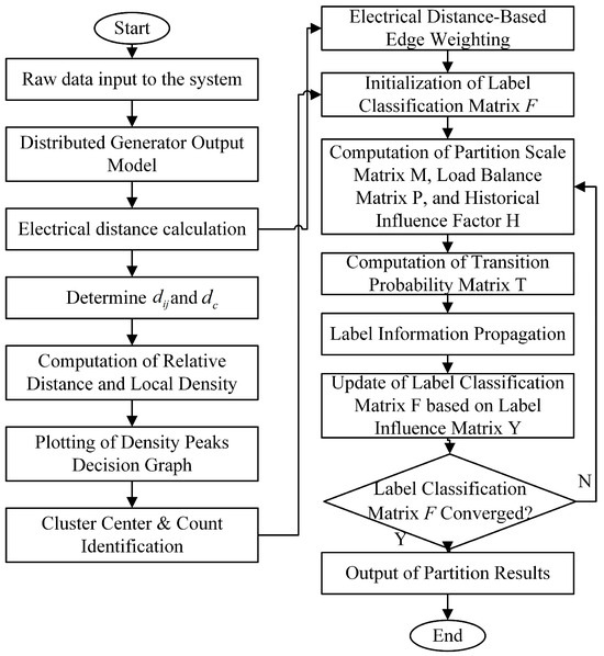
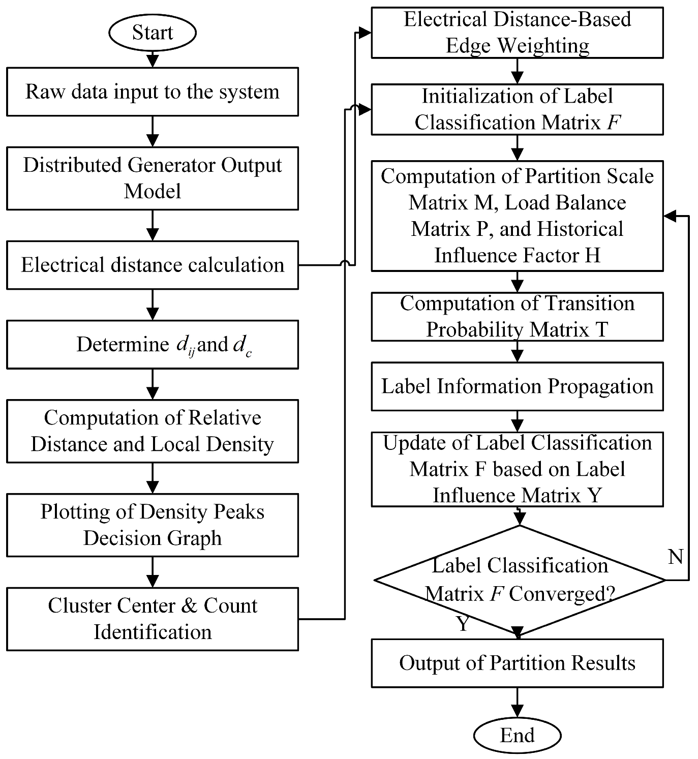
The complete partitioning workflow is shown in Figure 1.

Figure 1. Flowchart of the distribution network partitioning method based on the improved DPC-LPA approach.

5. Case Study Analysis

The method is assessed on actual medium- and low-voltage AC/DC distribution systems. Probability-distribution fitting first supplies the renewable operating point for each case. Because the 10 kV AC network has the most nodes, it is used to explain the distance calculation, DPC initialization, and LPA refinement in detail; the other three networks are used to examine applicability across voltage levels and AC/DC configurations. All numerical calculations, including probability-distribution fitting, power-flow analysis, voltage-sensitivity calculation, and DPC-LPA implementation, were performed using MATLAB R2020a (The MathWorks, Inc., Natick, MA, USA).

5.1. Case Study Baseline Data and Distributed Power Source Output Calculation

Historical wind speed and irradiance records are fitted to the selected distributions, and the representative values are converted into planned source outputs. These outputs, together with the network and load data, define the steady-state operating point for partitioning.

5.1.1. Wind Speed Probability Interval Statistics and Typical Value Selection

Assuming uniform wind speeds across the study area and identical wind turbine configurations, the rated, cut-in, and cut-out wind speeds are 12, 2, and 18 m/s, respectively. Historical wind speed data from 2022 were sampled at five-minute intervals, yielding 105,120 observations. The Weibull parameters were estimated from this data set by maximum likelihood.

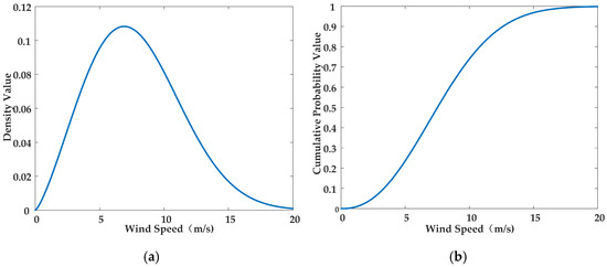
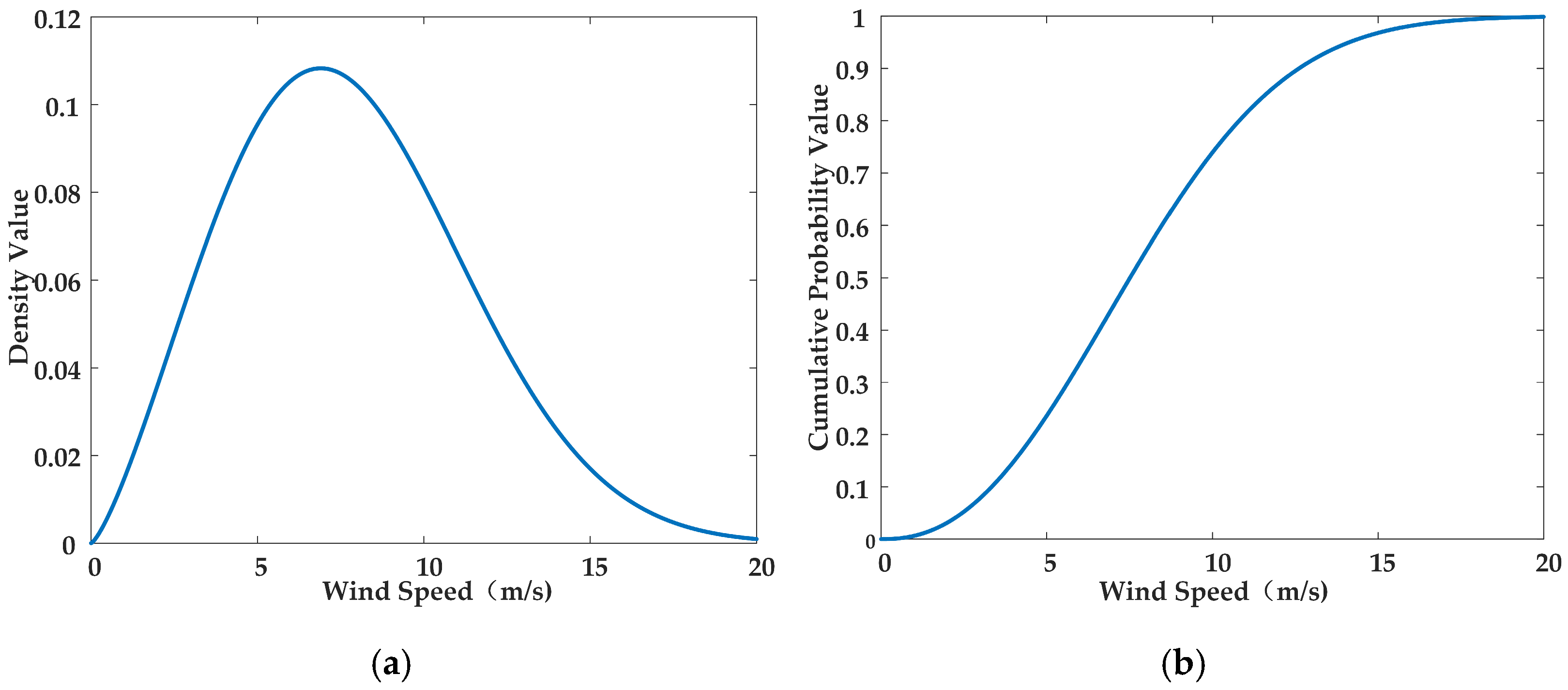
The annual wind speed sample was fitted to a Weibull distribution by maximum likelihood, giving scale parameter $c=8.801$ and shape parameter $k=2.3206$. The fitted PDF and CDF are shown in Figure 2.

Figure 2. Wind speed distribution based on the Weibull distribution. (a) Probability Density Distribution of Wind Speed; (b) Cumulative Distribution of Wind Speed.

Figure 2a shows a unimodal wind speed distribution, with the highest frequencies at 5–7 m/s; observations above 18 m/s are rare. The 2–18 m/s grid-connection range was divided into eight equal intervals, and the corresponding probabilities are listed in Table 1.

Table 1. Wind speed probability table.

Wind Speed (m/s)	Probability	Wind Speed (m/s)	Probability
(2, 4]	11.523%	(10, 12]	13%
(4, 6]	19.08%	(12, 14]	7.65%
(6, 8]	21.44%	(14, 16]	3.36%
(8, 10]	18.82%	(16, 18]	1.43%

The 4–6 and 6–8 m/s intervals contain 40.52% of the observations. The 5–7 m/s interval contains 21.25%; a representative value of 6.5 m/s is used to calculate the electrical distance matrix.

5.1.2. Solar Irradiance Interval Statistics and Typical Value Selection

Solar irradiance is assumed uniform across the study area, and the PV plants are assumed to share the same specifications. Rated irradiance is 500 W/m². Nighttime observations (0 W/m²) are excluded, and the remaining values are normalized by 1000 W/m².

The uniform-resource assumption assigns the same meteorological input to installations of the same type and is only a screening approximation for a geographically compact study area. Spatial wind/irradiance gradients, local shading or wake effects, and heterogeneous equipment can change the nodal injection vector and therefore shift electrical distances and zone boundaries. In practical deployment, node-specific meteorological series and equipment parameters should be fitted separately and supplied as a spatial scenario vector. The present data do not support a quantitative estimate of this spatial-aggregation bias.

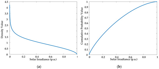
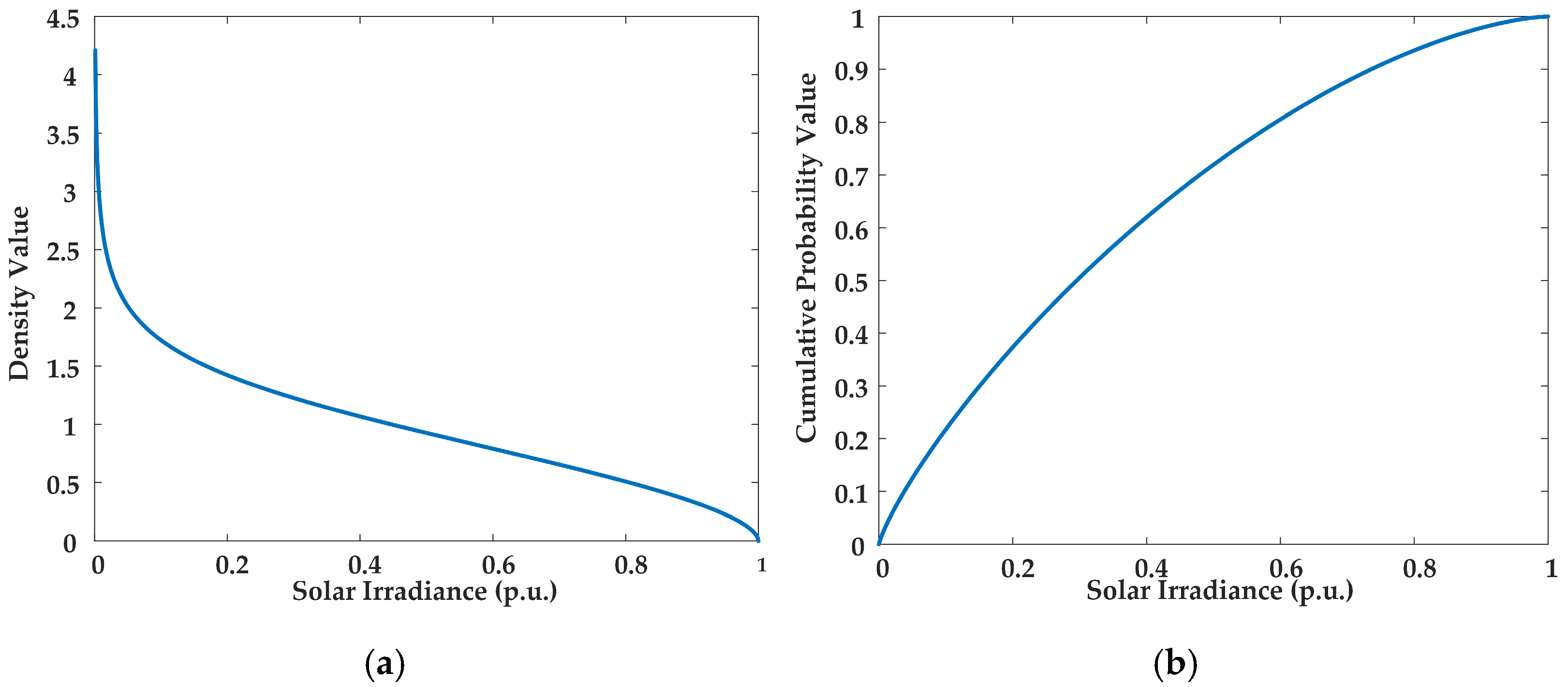
The annual solar irradiance sample was fitted to a Beta distribution, giving mean $\mu =0.3441$ and variance ${\sigma }^2=0.0668$. These statistics determine the shape parameters $\alpha =0.8185$ and $\beta =1.5602$. The fitted PDF and CDF are shown in Figure 3.

Figure 3. Beta-distributed solar irradiance distribution. (a) Probability density distribution of solar irradiance; (b) Cumulative distribution of solar irradiance.

Figure 3a shows a decreasing irradiance density, with its highest density near zero normalized irradiance. The range was divided into ten equal intervals; their probabilities, obtained from Figure 3b, are listed in Table 2.

Table 2. Solar irradiance probability table.

Solar Irradiance Standardized Value	Probability	Solar Irradiance Standardized Value	Probability
(0.0, 0.1]	21.77%	(0.5, 0.6]	8.59%
(0.1, 0.2]	15.59%	(0.6, 0.7]	7.22%
(0.2, 0.3]	13.21%	(0.7, 0.8]	5.77%
(0.3, 0.4]	11.35%	(0.8, 0.9]	4.31%
(0.4, 0.5]	10.07%	(0.9, 1.0]	2.12%

Table 2 shows that the interval (0, 0.1] has the largest probability, 21.77%, corresponding to 0–100 W/m². Its midpoint, 50 W/m², is therefore used as the representative irradiance in the electrical distance calculation.

5.1.3. Distributed Power Source Planning Output Results Based on Typical Scenarios

The planned output of each distributed source was calculated from its rated power and the representative meteorological condition. The resulting inputs for the partitioning calculation are listed in Table 3.

Table 3. Distributed power source planning output.

Power Source Name	Source Type	Common Weather Conditions	Rated Power (kW)	Planned Output Power (kW)
WT1	Wind	6.5 m/s	160	72
WT2			100	45
PV1	Solar	50 W/m2	100	10
PV2			150	15
PV3			50	5
PV4			30	3

5.1.4. Voltage-Level-Based Individual Zoning Scheme and Power Supply Configuration

The AC and DC subsystems at different voltage levels are partitioned separately to simplify voltage control and support local power balancing.

The rated capacities and connection nodes of the distributed sources in each subsystem are summarized in Table 4.

Table 4. Distributed power source parameters.

Distribution Network Type	Power Source Node	Power Source Name	Power Source Type	Rated Power (kW)
10 kV DC Distribution Network	10	WT2	Wind	160
10 kV AC Distribution Network	6	PV2	Solar	100
	17	WT1	Wind	200
	25	PV3	Solar	150
750 V DC Distribution Network	3	PV1	Solar	50
380 V AC Distribution Grid	3	PV4	Solar	30

5.2. Case Study Verification and Results for the Improved DPC-LPA Method

All four subsystems follow the same calculation sequence. The 37-node 10 kV AC network is examined in detail because it has the largest node set and the greatest load variation; the results for the remaining subsystems are then summarized using the same metrics.

The balance node is excluded from the iterative assignment because of its special operating role and is added afterward to the zone with the smallest electrical distance. Section 5.2.1, Section 5.2.2 and Section 5.2.3 present the distance matrix, initial centers, and final partition, respectively.

5.2.1. Verification of Comprehensive Electrical Distance Rationality

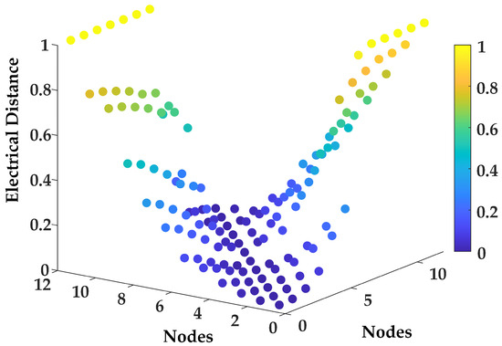
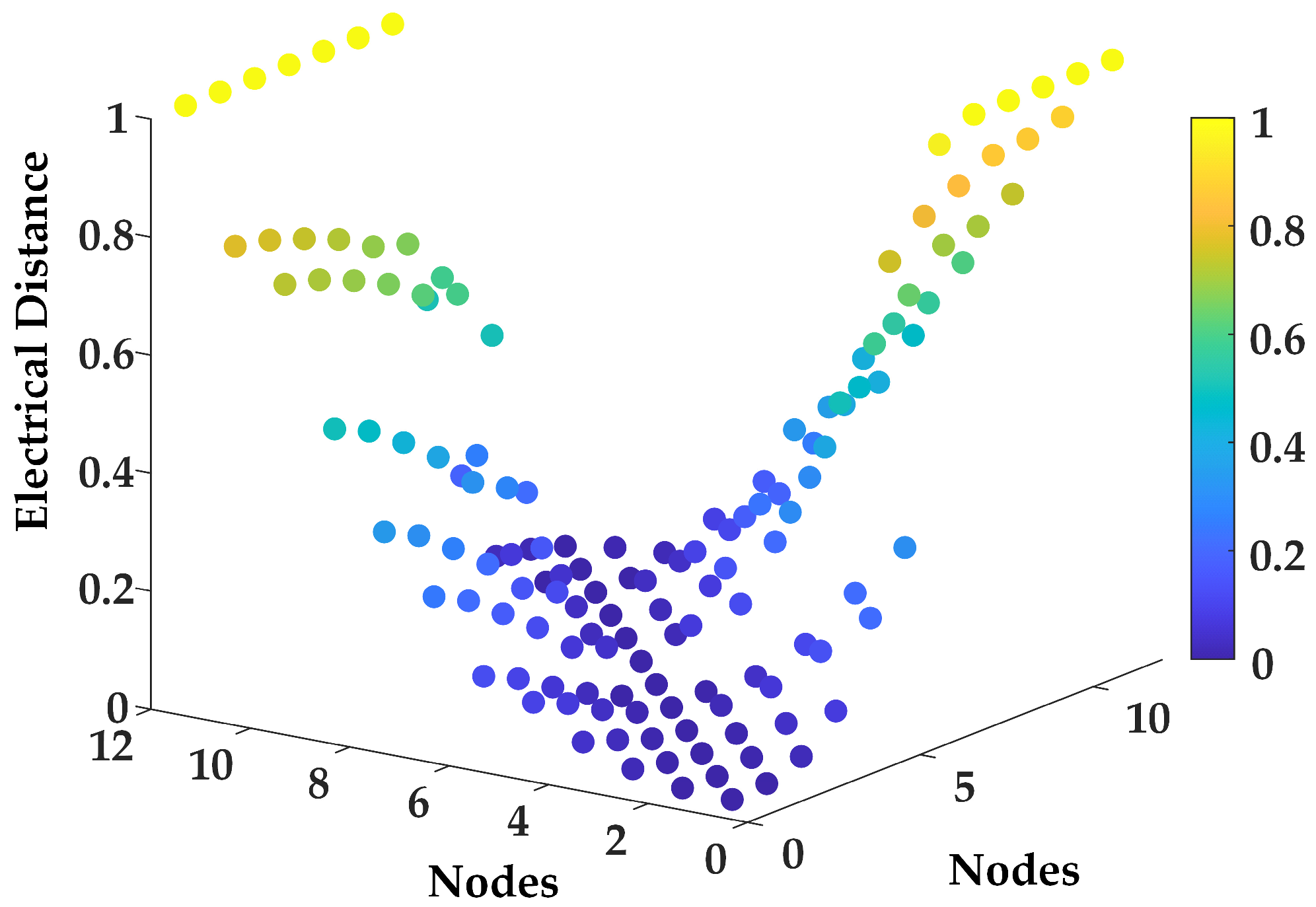
The node impedances and active- and reactive-power voltage-sensitivity matrices were calculated for the 10 kV AC network. Each pairwise comprehensive distance was evaluated with Equation (18) and mapped to a common [0, 1] scale with Equation (19). The resulting matrix is shown in Figure 4.

Figure 4. 10 kV AC distribution network node comprehensive electrical distance diagram.

Figure 4 shows the normalized distance surface. The surface is symmetric about the plane $y=x$, and its diagonal entries are zero. Equivalently, the comprehensive electrical distance between node $i$ and node j is equal to the comprehensive electrical distance between node j and node $i$, and the comprehensive electrical distance between node $i$ and node $i$ is zero, as required by a distance matrix.

Figure 4 confirms the symmetry, zero diagonal, and node-pair differentiation required of a distance matrix and is therefore interpreted as a physical-consistency check rather than comparative evidence. A controlled comparison against impedance-only and sensitivity-only distances should use identical topology, operating point, and DPC-LPA settings and evaluate modularity $Q$, balance score $B$, and within- and between-zone separation.

5.2.2. Initial Partitioning Based on DPC

DPC uses the normalized comprehensive distances to estimate the number and centers of zones. The remaining assignments depend on the cutoff distance $d_c$, so DPC is used only for initialization and the modified LPA performs the subsequent refinement.

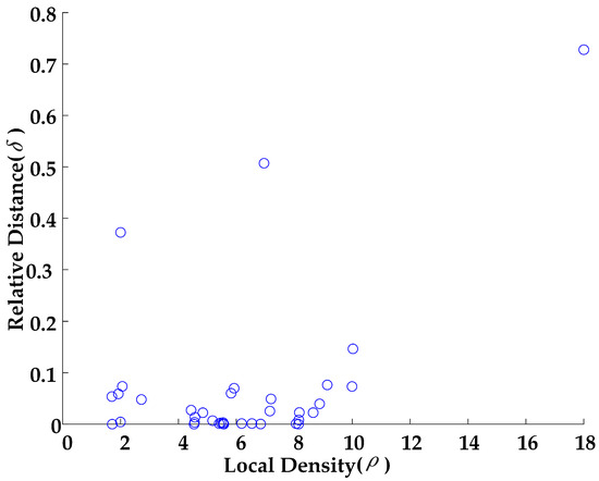
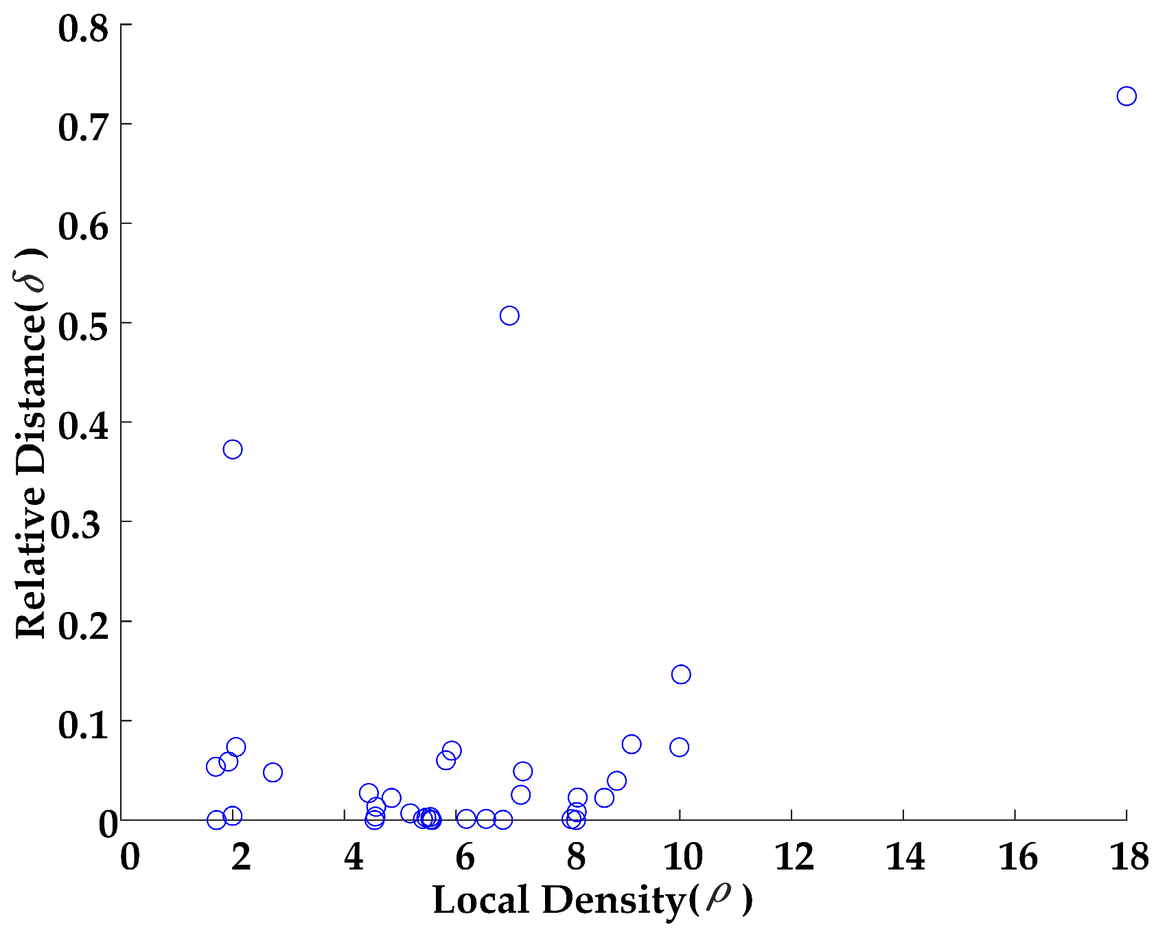
The local density $\rho$ and relative distance $\delta$ are calculated for all nodes and plotted as $x$ and $y$ coordinates to form the DPC decision graph in Figure 5.

Figure 5. DPC decision diagram for the 10 kV AC distribution network.

In Figure 5, three nodes have jointly high local density and relative distance and are selected as the initial centers. Using cutoff distance $d_c$, the remaining nodes are assigned to initialize the partition.

As shown in Table 5, nodes outside the cutoff neighborhoods of the three centers remain unassigned. The subsequent LPA stage therefore performs two tasks: assigning these nodes and revising boundary assignments under the balancing factors.

Table 5. Initialization of zones in a 10 kV AC distribution network.

Partition ID	Partition Center	Other Nodes in the Partition	Unpartitioned Nodes
1	25	2, 3, 4, 5, 28	1 (Balance node), 11, 12, 13, 14, 15, 20, 21, 22, 23, 24, 26, 27, 29, 30, 31, 32, 33, 36, 37
2	9	6, 7, 8, 10, 34, 35
3	17	16, 18, 19

5.2.3. Final Partitioning Based on Improved LPA

Starting from the DPC centers and preliminary labels, the modified LPA iteratively updates the remaining assignments. The partition-scale, load-balance, and historical-influence factors act during propagation to control zone growth, load disparity, and repeated switching. The following schemes isolate the effect of the LPA modification:

Scheme 1: Apply the traditional LPA to the DPC-initialized zones.

Scheme 2: Apply the improved LPA to the DPC-initialized zones.

The partitioning results for both schemes are presented in Table 6.

Table 6. Final zones obtained with the traditional and improved LPA schemes.

Scheme ID	Partition ID	Zone Center	Remaining Nodes in Zone	Zone Load Proportion	Modularity
Scheme 1	1	25	1, 2, 3, 4, 22, 23, 24, 26, 27, 28, 29, 30, 31	0.0789	0.5906
	2	9	5, 6, 7, 8, 10, 11, 12, 13, 32, 33, 34, 35, 36, 37	0.8075
	3	17	14, 15, 16, 18, 19, 20, 21	0.1136
Scheme 2	1	25	1, 2, 3, 4, 5, 22, 23, 24, 26, 27, 28, 29, 30, 31	0.0789	0.5796
	2	9	6, 7, 8, 10, 11, 32, 33, 34, 35, 36, 37	0.7273
	3	17	12, 13, 14, 15, 16, 18, 19, 20, 21	0.1939

The two schemes differ only in the assignments of nodes 5, 12, and 13. Scheme 1 places all three in Zone 2; Scheme 2 places node 5 in Zone 1 and nodes 12 and 13 in Zone 3. This redistribution reduces the concentration of nodes in Zone 2 and produces more comparable zone sizes.

The load proportions show the same pattern. Scheme 2 improves load balance while its modularity decreases slightly, indicating a trade-off between load distribution and topological cohesion rather than a loss of meaningful community structure.

A normalized balance score is used to quantify load balance:

$$B=1-{\displaystyle \frac{{\displaystyle \sum _k\left|p_k-\frac{1}{K}\right|}}{2\left(1-\frac{1}{K}\right)}},$$

(30)

where $p_k$ is the load proportion of zone $k$ and $K$ is the number of zones; $B=1$ indicates equal load shares. Using the values in Table 6, $B$ increases from 0.289 for Scheme 1 to 0.409 for Scheme 2, an improvement of 41.7%, while modularity changes only from 0.5906 to 0.5796. The result quantitatively shows the intended trade-off: the improved LPA substantially strengthens load balance with a modest modularity reduction.

Because the comparison uses one network and one parameterization, the 41.7% change is a deterministic case result rather than a statistical estimate. Repeated evaluations across parameters, operating scenarios, and topologies are needed to quantify dispersion. Modularity $Q$ and the balance score $B$ measure topological cohesion and load balance, respectively. Conductance could complement them with a boundary-cut measure, while normalized mutual information (NMI) is meaningful only when reference or consensus labels are available.

Classical K-means [25] is conceptually related but optimizes within-cluster Euclidean dispersion. Applying it to the present pairwise electrical distance data would require a prescribed K, a vector embedding, repeated initializations, and explicit connectivity post-processing. It is therefore not treated as a directly comparable baseline in the present study.

5.2.4. Low-to-Medium-Voltage AC/DC Distribution Network Partitioning Results

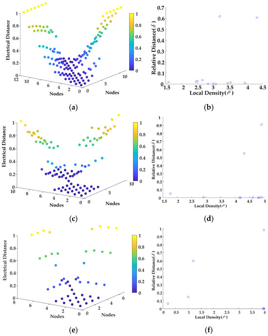
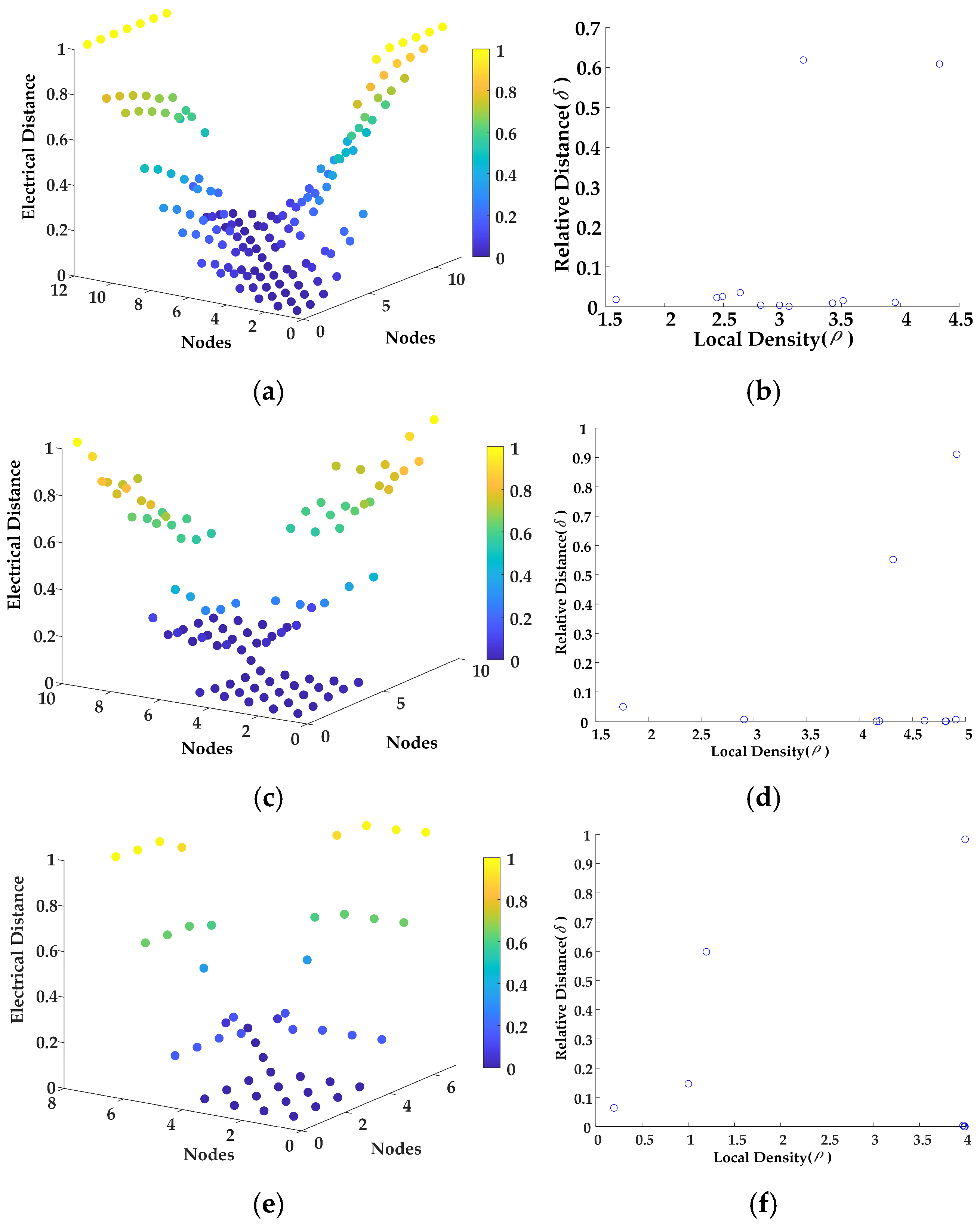
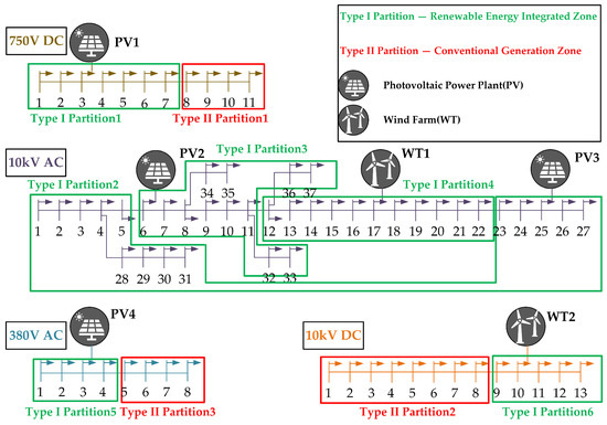
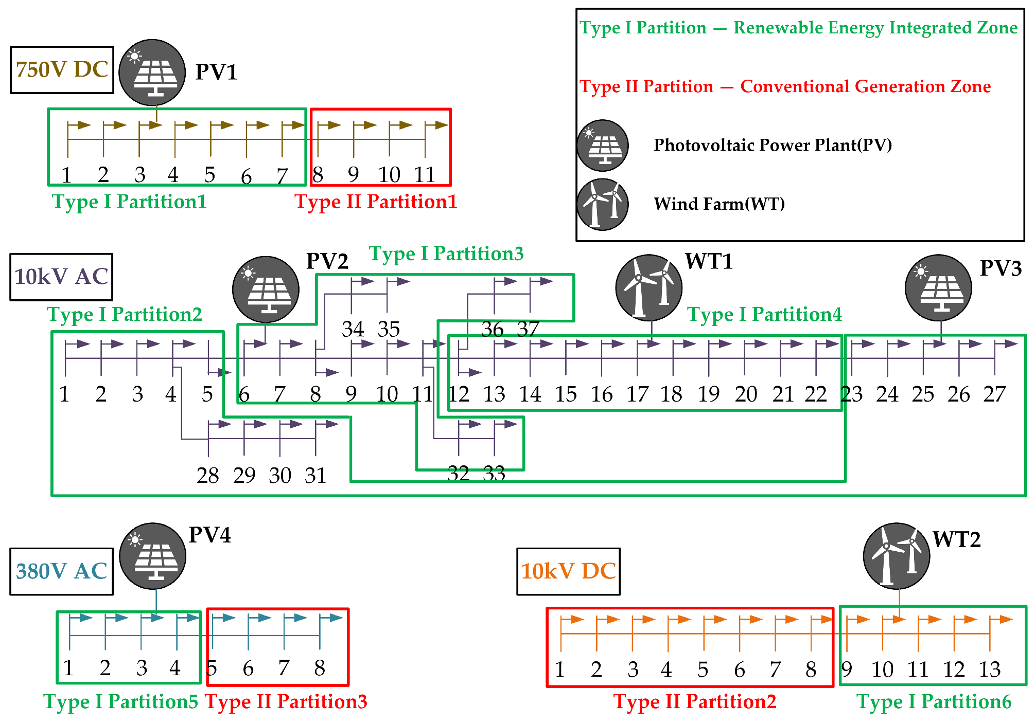
The improved DPC-LPA method was also applied to the 10 kV DC, 750 V DC, and 380 V AC distribution networks. Their comprehensive electrical distance surfaces and DPC decision diagrams are shown in Figure 6.

Figure 6. Comprehensive electrical distance and decision diagrams for each distribution network. (a) Comprehensive electrical distance map of nodes in the 10 kV DC distribution network; (b) DPC decision graph for the 10 kV DC distribution network; (c) Comprehensive electrical distance map of nodes in the 750 V DC distribution network; (d) DPC decision graph for the 750 V DC distribution network; (e) Comprehensive electrical distance map of nodes in the 380 V AC distribution network; (f) DPC decision graph for the 380 V AC distribution network.

The decision diagrams identify two zones and two center nodes for each of the three smaller networks. Their final partitions are shown in Figure 7.

Figure 7. Final partitioning results for medium- and low-voltage AC/DC distribution networks.

Figure 7 shows comparable zone sizes in all three networks. The associated load proportions and modularity values are listed in Table 7.

Table 7. Remaining distribution network zone information.

Distribution Network Type	Zone ID	Zone Center	Zone Load Proportion	Modularity
10 kV DC Distribution Network	1	5	0.4279	0.4793
	2	11	0.5721
750 V DC Distribution Network	1	3	0.4648	0.4691
	2	8	0.5352
380 V AC Distribution Network	1	4	0.5324	0.4722
	2	7	0.4676

Across the three two-zone networks, Table 7 reports comparable zone sizes, reasonably balanced load shares, and similar modularity values. These results extend the detailed 10 kV AC case to the tested 10 kV DC, 750 V DC, and 380 V AC systems, but they do not establish performance outside these networks.

The largest evaluated network contains 37 nodes, so large-scale performance remains unverified. For $n$ nodes, dense pairwise distance construction and standard DPC require $\mathcal{O}\left(n^2\right)$ time and memory, whereas each sparse LPA sweep is approximately $\mathcal{O}\left(\left|E\right|\right)$ and $I$ sweeps require $\mathcal{O}\left(I\left|E\right|\right)$, excluding the power-flow/Jacobian solution. The distance/DPC stage is therefore the principal scaling constraint. Larger-network studies should assess sparse solvers or candidate-pair screening and report runtime, memory, iteration count, and partition quality as $n$ increases.

5.3. Engineering Applicability and Geographical Limitations

The method evaluates partition rationality in the electrical and topological domains. Network impedance indirectly reflects conductor type and line length, but neither impedance nor voltage sensitivity represents terrain barriers, route accessibility, administrative boundaries, communication coverage, or maintenance constraints. The reported zones therefore do not establish geographical feasibility.

Applications in complex terrain require a two-stage workflow: DPC-LPA first identifies electrically cohesive candidate zones, after which geographical and operational feasibility is screened. Mandatory barriers can be represented as prohibited connections, while softer spatial preferences can be introduced as normalized edge penalties. The present data contain no geographical layer, so this extension remains to be validated.

The evaluated cases assume fixed topology and a converged normal steady state. Fault isolation, switching, islanding, or converter-control changes require the admittance model, coupled Jacobian, sensitivities, distance matrix, and partition to be recomputed. The workflow is therefore reusable across specified topologies but has not been validated for fault-time dynamics or real-time response. Contingency-specific precomputed partitions and assignment-consistency analysis are appropriate subjects for future work.

6. Conclusions

The proposed DPC-LPA workflow links three stages: representative renewable-scenario construction, comprehensive electrical distance calculation, and constrained label propagation. DPC determines the initial zone number and centers, whereas the partition-scale, load-balance, and historical-influence factors guide the subsequent LPA updates. In the tested AC/DC networks, the modified LPA improved load balance relative to traditional LPA while preserving similar modularity.

The formulation represents electrical and topological coherence but not geographical feasibility; incorporating geo-referenced penalties or hard constraints is a priority for future work. Further validation should examine probability-weighted multi-scenario partitions and common-protocol comparisons with alternative algorithms. The current evidence is limited to annual marginal resource fits, one dominant scenario, fixed normal topologies, networks of at most 37 nodes, and modularity/load-balance metrics. Future tests should therefore emphasize seasonal and spatial heterogeneity, abnormal topologies, and larger networks.

References

- Mo, J.S.; Song, N.; Fan, K.M. Optimization method for voltage deviation coefficient in partitioned distribution networks with high-proportion distributed PV. Electr. Power Constr. 2025, 46, 12–21. [Google Scholar]
- Zhao, L.; Ni, Y.; Zhao, S.; Yan, Q.; Wang, Y. Dynamic islanding division of AC/DC distribution networks with high penetration of distributed generation based on an improved fireworks algorithm. Power Supply Util. 2025, 42, 76–84. [Google Scholar]
- Zhang, Y.; Liu, Z.; Chen, Z. Smart-leader-based distributed charging control of battery energy storage systems considering SoC balance. Batteries 2023, 9, 18. [Google Scholar] [CrossRef]
- Zhang, Y.; Liu, Z.; Wang, F.; Chen, Z. Distributed power allocation scheme with prescribed performance and intermittent dynamics for BESSs with discharge rate constraints in microgrids. IEEE Trans. Syst. Man Cybern. Syst. 2025, 55, 1948–1959. [Google Scholar] [CrossRef]
- Chen, C.; Li, X.; Ji, K.; Wang, Y.; Lin, S. Cluster division and optimized operation of distribution networks considering source–load–storage matching. Electr. Power Constr. 2023, 44, 80–93. [Google Scholar]
- Chen, W.; Gan, W.; Zhang, J.; Yang, M.; Sun, L.; Liu, H. Hierarchical voltage regulation strategy for distribution networks based on HEM sensitivity. Electr. Power Constr. 2022, 43, 42–52. [Google Scholar]
- Xu, X.; Zhu, D.; Xu, X.; Wang, D.; Dai, X.; Wang, Y.; Yin, X. Coordinated control strategy for reactive power and voltage sensitivity in AVC substations of offshore wind power clusters. Electr. Meas. Instrum. 2025, 62, 53–64. [Google Scholar]
- Jiang, M.; Yan, W.; Xu, G.; Hong, H.; Zeng, X. Overvoltage control in active distribution networks based on integrated voltage sensitivity. Power Supply Util. 2023, 40, 9–14, 38. [Google Scholar]
- Liu, Y.; Ren, H.; Sun, C.; Liu, X.; Cao, Y. Distribution network partitioning method incorporating distributed PV based on AP clustering. Electr. Meas. Instrum. 2019, 56, 70–75. [Google Scholar] [CrossRef]
- Zhang, Y.; Shi, C.; Ye, P.; Ji, X.; Han, X.; Yang, M. Dynamic evaluation and early warning of voltage support capability in high penetration photovoltaic distribution networks based on sensitivity propagation theory. Proc. CSEE, 2025; early access. Available online: https://link.cnki.net/urlid/11.2107.TM.20250821.1814.018 (accessed on 5 August 2026).
- Ding, M.; Liu, X.; Bi, R.; Rong, X. Clustering method for high-penetration distributed power sources using comprehensive performance indicators. Autom. Electr. Power Syst. 2018, 42, 47–52. [Google Scholar]
- Li, X.; Xie, J.; Zhang, S. Two-stage robust control strategy for active voltage and reactive power in distribution networks based on clustering. Proc. CSEE 2025, 45, 7058–7071. [Google Scholar]
- Girvan, M.; Newman, M.E.J. Community structure in social and biological networks. Proc. Natl. Acad. Sci. USA 2002, 99, 7821–7826. [Google Scholar] [CrossRef] [PubMed]
- Newman, M.E.J.; Girvan, M. Finding and evaluating community structure in networks. Phys. Rev. E 2004, 69, 026113. [Google Scholar] [CrossRef] [PubMed]
- Bai, X.; Wu, H.; Yang, S.; Li, Z. Probabilistic production simulation of a wind/photovoltaic/energy storage hybrid power system based on sequence operation theory. IET Gener. Transm. Distrib. 2018, 12, 2700–2706. [Google Scholar] [CrossRef]
- Seguro, J.V.; Lambert, T.W. Modern estimation of the parameters of the Weibull wind speed distribution for wind energy analysis. J. Wind. Eng. Ind. Aerodyn. 2000, 85, 75–84. [Google Scholar] [CrossRef]
- Li, Y.; Lü, N.; Liu, X.; Hu, J.; Xu, Y. Power output evaluation method for distributed PV clusters considering new energy integration and grid losses. Electr. Power Constr. 2022, 43, 136–146. [Google Scholar]
- Shiga, T.; Kato, T.; Suzuoki, Y. Probabilistic solar irradiation forecast using beta regression: A study on capability of predicting large forecast error. IEEJ Trans. Power Energy 2014, 134, 527–536. [Google Scholar] [CrossRef]
- Liu, X. Research on Clustering Methods for High-Penetration Distributed Renewable Energy Generation. Master’s Thesis, Hefei University of Technology, Hefei, China, 2020. [Google Scholar]
- Zhang, Q.; Ding, J.; Zhang, D.; Wang, Q.; Ye, Q. Reactive power optimization for high-penetration distributed systems based on cluster partitioning. Autom. Electr. Power Syst. 2019, 43, 130–137. [Google Scholar]
- Raghavan, U.N.; Albert, R.; Kumara, S. Near linear time algorithm to detect community structures in large-scale networks. Phys. Rev. E 2007, 76, 036106. [Google Scholar] [CrossRef] [PubMed]
- Cordasco, G.; Gargano, L. Community detection via semi-synchronous label propagation algorithms. In Proceedings of the 2011 IEEE International Workshop on Business Applications of Social Network Analysis, Bangalore, India, 15 December 2011; pp. 1–8. [Google Scholar]
- Liu, H.; Zhou, S.; Gu, W.; Zhu, H.; Chen, Q.; Zhang, X. Identification and partitioning of critical nodes in power grids based on a network fault link matrix. Proc. CSEE 2025, 45, 4620–4633. [Google Scholar]
- Rodriguez, A.; Laio, A. Clustering by fast search and find of density peaks. Science 2014, 344, 1492–1496. [Google Scholar] [CrossRef] [PubMed]
- Lloyd, S.P. Least squares quantization in PCM. IEEE Trans. Inf. Theory 1982, 28, 129–137. [Google Scholar] [CrossRef]
Disclaimer/Publisher’s Note: The statements, opinions and data contained in all publications are solely those of the individual author(s) and contributor(s) and not of MDPI and/or the editor(s). MDPI and/or the editor(s) disclaim responsibility for any injury to people or property resulting from any ideas, methods, instructions or products referred to in the content. |
© 2026 by the authors. Licensee MDPI, Basel, Switzerland. This article is an open access article distributed under the terms and conditions of the Creative Commons Attribution (CC BY) license.