Voltage Scaled Low Power DNN Accelerator Design on Reconfigurable Platform

Abstract

The exponential emergence of Field-Programmable Gate Arrays (FPGAs) has accelerated research on hardware implementation of Deep Neural Networks (DNNs). Among all DNN processors, domain-specific architectures such as Google’s Tensor Processor Unit (TPU) have outperformed conventional GPUs (Graphics Processing Units) and CPUs (Central Processing Units). However, implementing low-power TPUs in reconfigurable hardware remains a challenge in this field. Voltage scaling, a popular approach for energy savings, can be challenging in FPGAs, as it may lead to timing failures if not implemented appropriately. This work presents an ultra-low-power FPGA implementation of a TPU for edge applications. We divide the systolic array of a TPU into different FPGA partitions based on the minimum slack value of different design paths of Multiplier Accumulators (MACs). Each partition uses different near-threshold (NTC) biasing voltages to run its FPGA cores. The biasing voltage for each partition is roughly calculated by the proposed static schemes. However, further calibration of biasing voltage is performed by the proposed runtime scheme. To overcome the timing failure caused by NTC, the MACs with higher minimum slack are placed in lower-voltage partitions, while the MACs with lower minimum slack paths are placed in higher-voltage partitions. The proposed architecture is implemented in a commercial platform, namely $Vivado$ with Xilinx $Artix\text{-}7$ FPGA and academic platform $VTR$ with 22 nm, 45 nm and 130 nm FPGAs. Any timing error caused by NTC can be caught by the Razor flipflop used in each MAC. The proposed voltage-scaled, partitioned systolic array can save 3.1% to 11.6% of dynamic power in $Vivado$ and $VTR$ tools, respectively, depending on the FPGA technology, partition size, number of partitions and biasing voltages. The normalized performance and accuracy of benchmark models running on our low-power TPU are very competitive compared to existing literature.

1. Introduction

The popularity of TPU-based neural network implementations is increasing due to shorter training times, faster inference, energy efficiency and scalability compared to CPU and GPU solutions [1]. Additionally, the integration of TensorFlow with TPU enables users to run their neural network models on TPUs without extensive modifications to their code. On the other hand, the configurable logic block (CLB) and switch matrix of FPGAs are power-hungry, which makes FPGAs energy-inefficient when compared to ASICs. Recently many researchers [2,3] have reported CPU-FPGA-based hybrid data center architectures, which provide hardware acceleration facility for deep neural networks (DNNs). Despite power inefficiency, FPGA has become popular in the cloud-scale acceleration architecture due to its computational efficiency, specialized hardware and the economic benefits of homogeneity. Therefore, reducing power in FPGA for DNN applications becomes a very relevant topic of research.

1.1. Literature

B Salami et al. [4] studied the timing failure vs. biasing voltage of a DNN implementation in FPGA. They under-scaled the biasing voltage ($V_{ccint}$) of the entire FPGA to increase the power efficiency of the convolutional neural network (CNN) accelerator by a factor of 3. A single $V_{ccint}$ for the entire FPGA might not be the most power-efficient solution. Partitioning an FPGA according to the slacks and feeding different biasing voltages for different partitions can cause a further reduction in power for CNN implementations. In [5], the authors implemented a systolic array using a near-threshold (NTC) biasing voltage in an ASIC, which can predict the timing failure of multiplier accumulators (MACs) placed inside the systolic array of a TPU. The prediction of timing failure is based on $Razor$ flipflop [6]. Higher fluctuation of input bits increases the possibility of timing failure in NTC conditions. In [5], once the timing failure of a MAC was predicted by its internal $Razor$ flipflop, the biasing voltage of the MAC was boosted. In the literature, there are three types of timing error controlling techniques used to predict timing errors for systolic arrays.

1.1.1. Timing Error Detection and Recovery (TED)

TED was first proposed in [7], the authors of which used Razor flipflops to sample the outputs. The outputs are executed by a regular clock and a delayed clock. If the outputs from these two different clocks are different, an error flag is indicated, and the inputs are re-executed with a reduced clock frequency. The TED scheme has three variants, as follows: TED Clock Gating (TEDCG), TED Counterflow(TEDCF) and TED Rollback (TEDRB) [8].

1.1.2. Timing Error Propagation (TEP)

Timing Error Propagation (TEP) [8] allows timing errors to propagate subsequent computation stages instead of re-executing inputs of erroneous MACs. TEP expects the algorithm itself to be error-resilient. This approach explores the noise tolerance of the algorithm. The authors of [8] showed the accuracy of DNN falls when the timing error rate crosses 0.1%. The authors of [9] showed that algorithmic noise tolerance (ANT) hardware can tolerate a 21.3% error rate, with performance degradation of only 3.5% at a 97.4% overhead.

1.1.3. Timing Error Drop (TE-Drop)

Like TED, Timing Error Drop [5,10] also uses $Razor$ flipflop to detect timing error. However, Unlike TED, TE-Drop can recover timing errors without re-executing the logic of fallacious MACs. TE-Drop shows that weight distribution is biased towards small values. Therefore, the logical participation of individual MACs to output neurons is very insignificant. When a MAC detects a timing error, TE-Drop steals the next clock cycle from its previous MAC to compute the correct partial sum and drops the update of the previous MAC. TE-Drop uses an MUX, which is controlled by an error flag from the previous MAC. If the previous MAC detects error, the MUX passes the sum correctly computed partial by the $Razor$ flipflop; otherwise, the current MAC passes the actual partial sum. Table 1 shows different neural network architectures.

Table 1. Comparison with the literature.

	Static	Runtime		Runtime	Name of		Transistor	Power Reduction	Remarks
Paper	Offline Calibration	Error Correction (REC)	Error Prediction and Correction (REPC)	Error Detection	Error Correction Technique	Platform	Technology	Strategy
J. Zhang et al. [10], 2018	×	×	×	🗸	TE-Drop	ASIC	45 nm	Underscaling single $V_{ccint}$	Underscaling of $V_{ccint}$, accuracy study of DNN, $Razor$-based timing error detection, correction with TE-Drop
Pandey er al. [5], 2019	×	×	🗸	🗸	TE-Drop	ASIC	15 nm	Underscaling multiple $V_{ccint}$	Underscaling of $V_{ccint}$, accuracy study of CNN, $Razor$-based timing error detection, heuristic error prediction, correction with TE-Drop
Salami et al. [4], 2020	×	×	×	×	×	Xilinx ZCU-102 FPGA	16 nm	Underscaling single $V_{ccint}$	Underscaling of $V_{ccint}$, accuracy study of CNN
Ernst et al. [7], 2006	×	×	×	🗸	TED	ASIC	180 nm	Underscaling single $V_{ccint}$	Underscaling of $V_{ccint}$, accuracy study of DNN, $Razor$-based timing error detection, correction with TED
Jiao et al. [8]	×	×	×	🗸	TEP	ASIC	45 nm	Underscaling single $V_{ccint}$	Underscaling of $V_{ccint}$ with variation of temperature, changing training set accuracy study of CNN
Azghadi et al. [11], 2020	×	×	×	×	×	Virtex-VU9 FPGA	28 nm	Architectural optimization	Resource-optimized hardware architecture for DNN
Zhao et al. [12], 2020	×	×	×	×	×	Intel Aria10 FPGA	18 nm	Architectural optimization	Resource-optimized hardware architecture for CNN, accuracy study of CNN
Kim et al. [13], 2020	×	×	×	×	×	Xilinx Zynq FPGA	28 nm	Clock gating	Low-power CNN architecture, clock gating used to optimize power
Duvindu et al. [14], 2020	×	×	×	×	×	Xilinx Zynq FPGA	28 nm	Clock gating	Power savings with minimal accuracy and performance loss
Pandey et al. [15], 2021	×	×	×	×	×	ASIC	15 nm	Power gating	It addresses a significant hardware underutilization problem in weight-stationary systolic arrays
Our	🗸	🗸	🗸	🗸	TE-Drop	Xilinx Artix 7 FPGA	28 nm	Underscaling multiple $V_{ccint}$	Underscaling of $V_{ccint}$, partitioning FPGA based on critical paths of MACs, accuracy study of DNN, $Razor$-based timing error detection, heuristic error prediction, correction with TE-Drop

The authors of [11,12,13,14] implemented power-optimized hardware accelerators for neural networks on FPGA platforms. These hardware accelerators optimized power consumption through clock gating and various conventional architectural optimization approaches. The authors of [15] reduced power consumption of TPUs on a 15 nm ASIC platform using a power gating methodology. However, these articles did not explore voltage underscaling approaches. The authors of [4] explored underscaled biasing voltage for CNNs on FPGA platforms but did not address timing error detection and correction measures. Conversely, the authors of [5,7,8,10] focused on ASIC implementations of neural networks and underscaled biasing voltage and also investigated solutions for timing error detection and correction. As shown in Table 1, refs. [7,8] used TED and TEP, respectively. However, refs. [5,10] used TE-Drop to correct runtime timing errors.

1.2. Contribution

Targeting FPGA-based DNN applications [2], our work investigates voltage scaling techniques for systolic arrays in TPUs on the FPGA platform, employing the TE-Drop error correction method. Similar to ASICs, implementing different $V_{ccint}$ values for each of the MACs in a systolic array is unrealistic for FPGA platforms. Therefore, this work partitions the FPGA floor according to the minimum slack value of design paths of MACs. Each partition consists of a group of MACs with similar minimum slacks. Each partition is connected with different $V_{ccint}$ values. The proposed methodology abstracts the synthesis timing report from the $Vivado$ and $VTR$ tools. In a synthesized design, the $Vivado$ and $VTR$ timing engines estimate the net delays of paths based on connectivity and fanout. The clustering algorithms create clusters or groups based on the minimum slack of all MACs. The clusters consist of MACs that have lower minimum slacks placed in FPGA partitions with higher $V_{ccint}$ values and clusters of MACs with higher minimum slacks placed in FPGA partitions with lower $V_{ccint}$ values. Here, the $V_{ccint}$ provides power to an FPGA core. The timing errors caused in the proposed systolic array for the $V_{ccint}$ values are handled a Timing Error Control Unit (TECU) using $razor$ flipflop. By discarding the MAC operation after an incorrect MAC due to timing errors and using the additional clock cycle to accurately compute the incorrect MAC’s result, TE-Drop prevents the performance penalty of re-execution. The tuning of $V_{ccint}$ with slack is performed by unique $static$ and $runtime$ strategies. The circuit-level challenges in the implementation of voltage scaling in the FPGA platform are beyond the scope of our article. However, the feasibility of implementing the necessary hardware for voltage scaling support is evident, considering the successful implementations in other ASIC technologies. Due to the unavailability of multiple $V_{ccint}$ supports in a single FPGA device, our entire design with multiple partitions cannot be implemented on FPGA. However, for the proof of concept, the design is implemented on FPGA with one partition at a time. The power measurements are performed using the Xilinx $Vivado$ probe. Furthermore, the timing parameters are taken from synthesis and implementation processes, which take into account the actual timing reality of FPGA devices. On the other hand, the $VTR$-based results are taken from simulation. The proposed method does not impact the logic of design paths. Hence, it can be implemented in any existing low-power neural network architecture for additional power reduction. The contributions of this paper are described as follows:

• This paper proposes a new CAD flow to create voltage-scaled TPUs on FPGA-based platforms considering the trade-off between circuit delay and biasing voltage. The proposed CAD flow can be used in any existing low-power neural network architecture for additional power reduction.
• The cluster algorithms divide the systolic array of a TPU into different partitions (groups or clusters) based on the minimum slacks (critical paths) of MACs. Instead of applying uniform $V_{ccint}$ across all MACs in the systolic array, the group of MACs with shorter critical paths is connected with lower $V_{ccint}$, and the group of MACs with longer critical paths is connected with higher $V_{ccint}$.
• The calibration of the $V_{ccint}$ of different partitions is performed by the proposed $runtime$ and $static$ schemes. The timing errors caused by voltage reduction are detected by a heuristic-based timing error prediction method.

The organization of this article is described as follows. Section 2 outlines our background of the FPGA environment. The working principle of $Razor$ flipflop to detect runtime timing failure is discussed in Section 2.5. The methodology of the proposed work is described in Section 3. Section 4 discusses the clustering algorithms. Results of the implementation and conclusions are presented in Section 5 and Section 6, respectively.

2. Background: FPGA Environment

The proposed scheme was implemented in Xilinx FPGAs using the $Vivado$ commercial tool flow and in academic FPGAs using $VTR$ CAD tools. In our first approach, we used the Xilinx $Vivado$ tool with an Artix-7 FPGA and the $VTR$ tool flow with 22 nm, 45 nm and 130 nm academic FPGAs. The $VTR$ supports $Vc{c}_{int}$ in the critical voltage region, which is not available in $Vivado$.

2.1. Vivado Environment

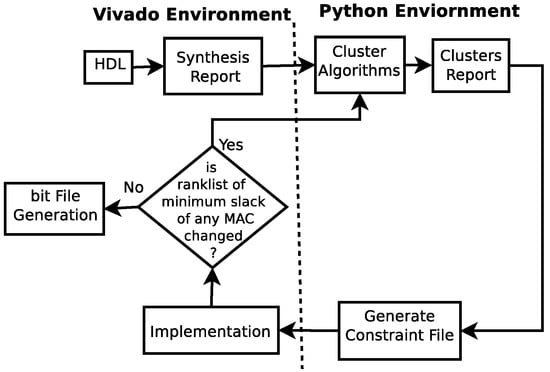
A typical Xilinx FPGA in the $Vivado$ environment has three conventional steps, namely synthesis, implementation and bit file generation, whereas the adopted tool flow of the proposed partitioned FPGA is divided into the following two environments: (i) the $Vivado$ environment for synthesis, implementation and bit file generation and (ii) the Python environment for clustering of similar slacks. The entire tool flow is shown in Figure 1. The $Vivado$ environment involves the following three sub-steps:

Figure 1. Vivado tool flow.

2.1.1. Synthesis

The $Vivado$ synthesis process transforms register transistor logic (RTL) to a gate-level representation. The synthesis process generates delays of all possible paths of the design. The timing report of the synthesis process contains 12 pieces of information, namely the name of the path, slack value, level, high fanout, path from, path to, total delay of path, logic delay, net delay, time requirement source clock and destination clock. It is to be noted that the estimation of the slacks of each logic block is performed at a high level. The actual timing behavior of the design depends on the net delays after placement and routing.

2.1.2. Implementation

The $Vivado$ implementation process is a timing-driven flow that transforms a logical netlist and constraints (Xilinx design constraints format) into a placed and routed design to make it ready for the bitstream generation process. In our proposed tool flow, the logical netlist is provided by the $Vivado$ synthesis process, but the Xilinx Design Constraints (XDCs) are generated by a Python script. The clustered MACs are considered for placement in a specific location on the FPGA floor.

2.1.3. Bit File Generation

Once placement and routing are completed by the implementation process, the flow generates a bitstream of the systolic array. The Xilinx bitstream generation program produces a bitstream for Xilinx device configuration. CPUs typically accompany TPUs as hardware accelerators. CPUs in this context are responsible for providing application libraries and input data to the TPU.

2.2. VTR Environment

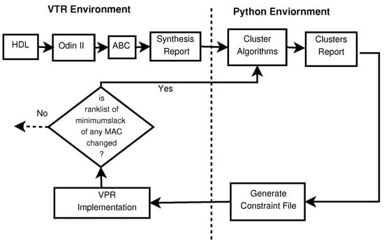
In a commercial CAD environment, biasing voltage is fixed. The Verilog to Routing (VTR) [16] tool is an open-source academic CAD tool flow for the FPGA architecture that allows for voltage scaling technology. The $VTR$ contains three separate tools, namely Odin II [17], ABC [18] and VPR [19]. The entire tool flow is shown in Figure 2. The $VTR$ environment involves the following three sub-steps.

Figure 2. VTR tool flow.

2.2.1. Synthesis

The synthesis process of the proposed $VTR$ tool flow is processed by $OdinII$ and $ABC$. $OdinII$ elaborates and synthesizes HDL into FPGA architectural primitives like FFs, multipliers and adders. Thereafter, the circuit logic is handled by $ABC$ to perform technology-independent logic optimizations; then, the technology maps the soft logic to LUTs. The information in the timing report generated by $ABC$ is similar to the $Vivado$ synthesis report. The different slack values of different design paths in the synthesis report are used in cluster algorithms.

2.2.2. Implementation

The $VPR$ [19] tool is a part of the $VTR$ flow, which is used for the physical implementation of the circuit in the target FPGA architecture, along with Synopsys Design Constraint (SDC) file . In the $VTR$ flow, the logical netlist is provided by $OdinII$ and the $ABC$ synthesis process, but the SDC is generated by a Python script. The clustered slack values generated by the Python script are considered for placement of the logic paths in a specific location on the FPGA floor. At the end, $VPR$ analyzes the circuit implementation to generate area, speed and power data, as well as a post-implementation netlist. Many commercial CAD tools like Titan Flow use Intel’s Quartus, while Yosys uses $VPR$ for logic synthesis, optimization and technology mapping.

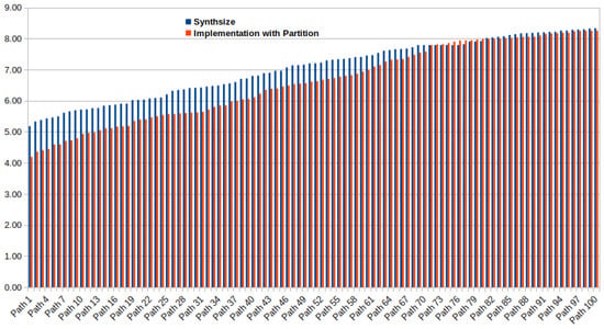
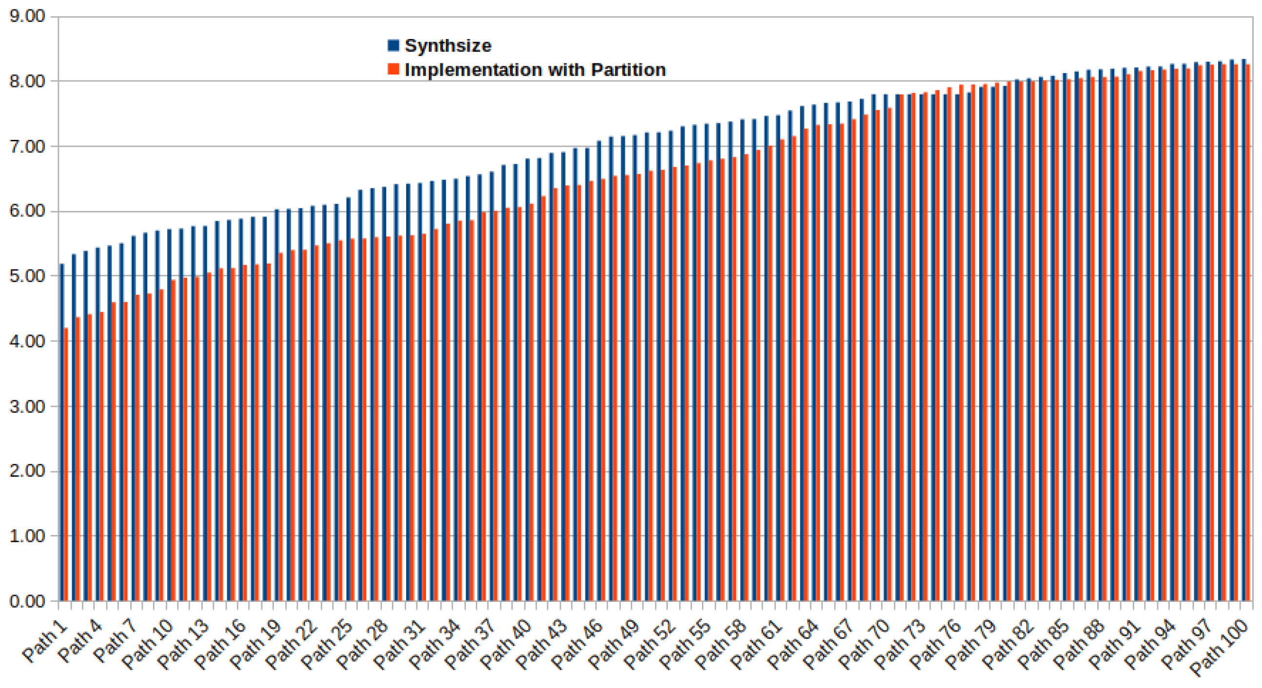
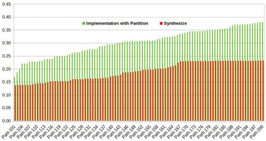
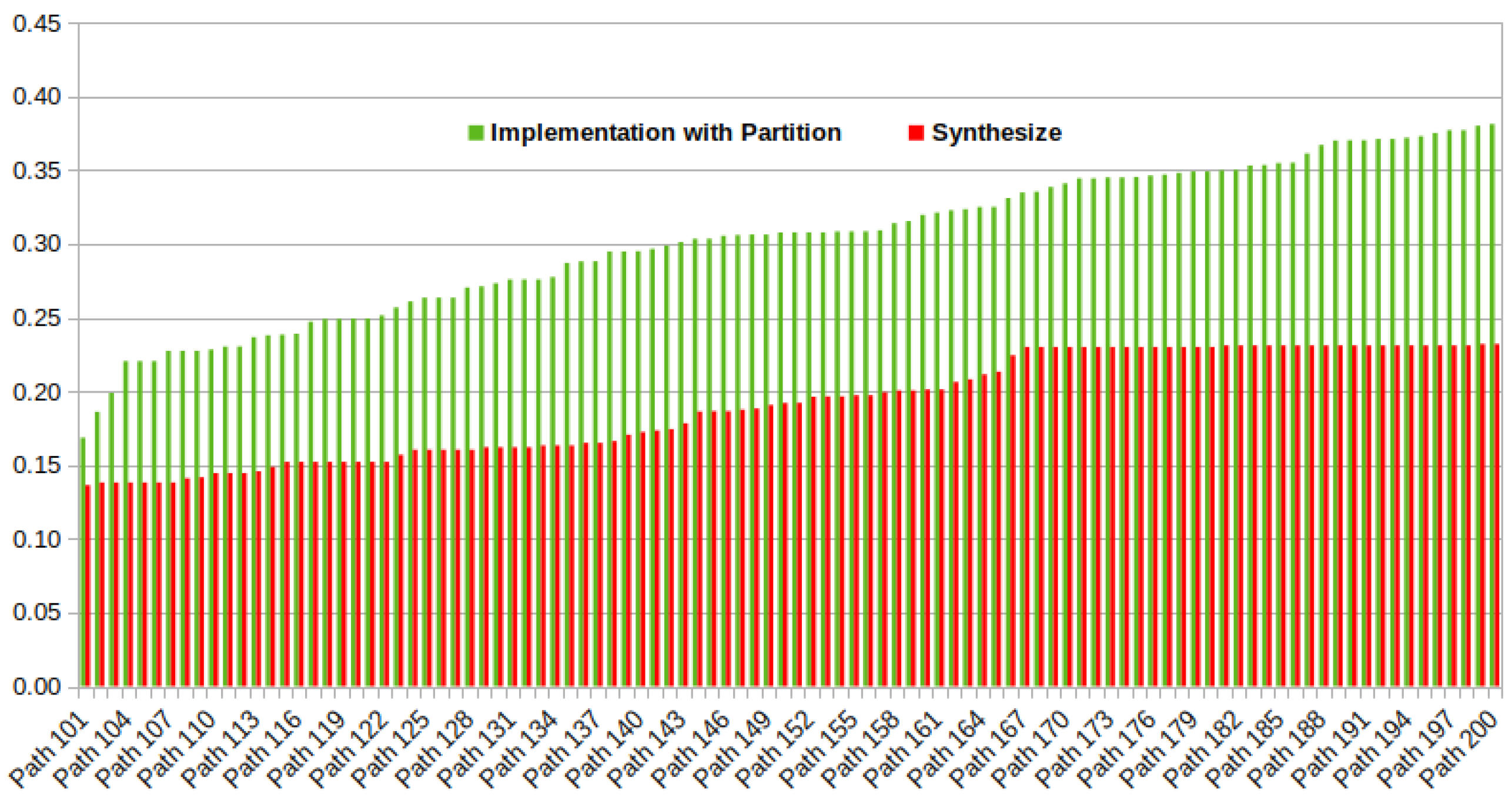
There is a possibility that after the partitioning of the systolic array, delays of design paths from the implementation process may differ from delays of design paths from the synthesis process. Therefore, changes in the delay of the design path may affect the minimum slack of MACs; as a consequence, the entire design needs to re-cluster based on the new minimum slacks of MACs. Figure 3 and Figure 4 report the differences in delays of the 100 worst design paths of the synthesis process and the implementation (after partition) process, respectively. Figure 3 and Figure 4 show that the partitioning process does not affect the design paths significantly. The proportional changes in the delays of design paths in Figure 3 and Figure 4 affect the minimum slacks of MACs in each partition proportionally. Therefore, the rank list of design paths based on minimum slack remains unaffected and the partition process remains unchanged.

Figure 3. Slacks of the 100 worst setup paths in Vivado for a 16 × 16 systolic array.

Figure 4. Slacks of the 100 worst hold paths in Vivado for a 16 × 16 systolic array.

2.3. Python Environment

The contribution of this paper lies in augmenting the standard FPGA design tool flow by incorporating a Python-based environment, which consists of a script to run three subsequent processes, namely the choice of $ClusteringAlgorithms$, $ClusterGeneration$ and $ConstraintGeneration$.

2.3.1. Choice of Clustering Algorithms

A clustering algorithm suited to the requirements is chosen at this step. As stated in Section 3, this paper investigates four commonly used clustering algorithms, namely hierarchical, K-means, mean-shift and DBSCAN algorithms.

2.3.2. Cluster Generation

We assume that the FPGA is divided into a few partitions and each partition has a different biasing voltage ($V_{ccint}$). The clustering algorithms create few groups of MACs. The MACs with similar minimum slacks form a group, and they are placed in the same FPGA partition. It is to be noted that groups of MACs and clusters are represented using rectangle or square shapes, respectively, for improved readability and comprehension.

2.3.3. Constraint Generation

Xilinx uses a constraint file format (XDC) to specify the coordinates of different paths of the proposed systolic array. The XDC file is generated by the Python script.

2.4. Clustering MACs Based on Their Minimum Slacks

The idea of voltage scaling for a partitioned systolic array was initially based on the slacks generated from the synthesis report. Slack-based clustering can group different or similar design paths belonging to different MACs, which may be placed in the different physical locations of the FPGA floor by the placement and routing algorithm. For the slack-based design path partitioning approach, the intervention of the proposed tool script is far greater than the placement and routing process of existing EDA tools. As a result, the timing parameters reported by the synthesis process are varied significantly after the placement and routing process of existing EDA tools at the implementation level. For four partitions with a 16 × 16 systolic array, the $Vivado$ tool generates a 4.23 ns critical path. The same design has a 11.93 ns critical path after placement routing, which is almost two times the critical path generated from the synthesis report. We note that the placement and routing process of slack-based partitioning of a 64 × 64 systolic array takes 10 to 14 h on an i5, 8 GB Linux platform. Later, instead of clustering design paths based on slack, clustering is performed on MACs using their minimum slack values. We find that clustering MACs based on their minimum slack is reasonable and better compared to the previous method for the following reasons:

• For the clustering of MACs based on their minimum slack, the intervention of the vendor’s technology-dependent placement and routing algorithm is far greater compared to the previous idea. As a result, the critical path variation in the synthesis and implementation process is very minimal.
• Placing all design paths in a constraint file is much more complicated compared to placing entire MACs in a constraint file.
• The routing of wires on the FPGA floor is comparatively simpler for MAC clustering based on their minimum slacks.

2.5. Razor Flipflop

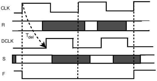
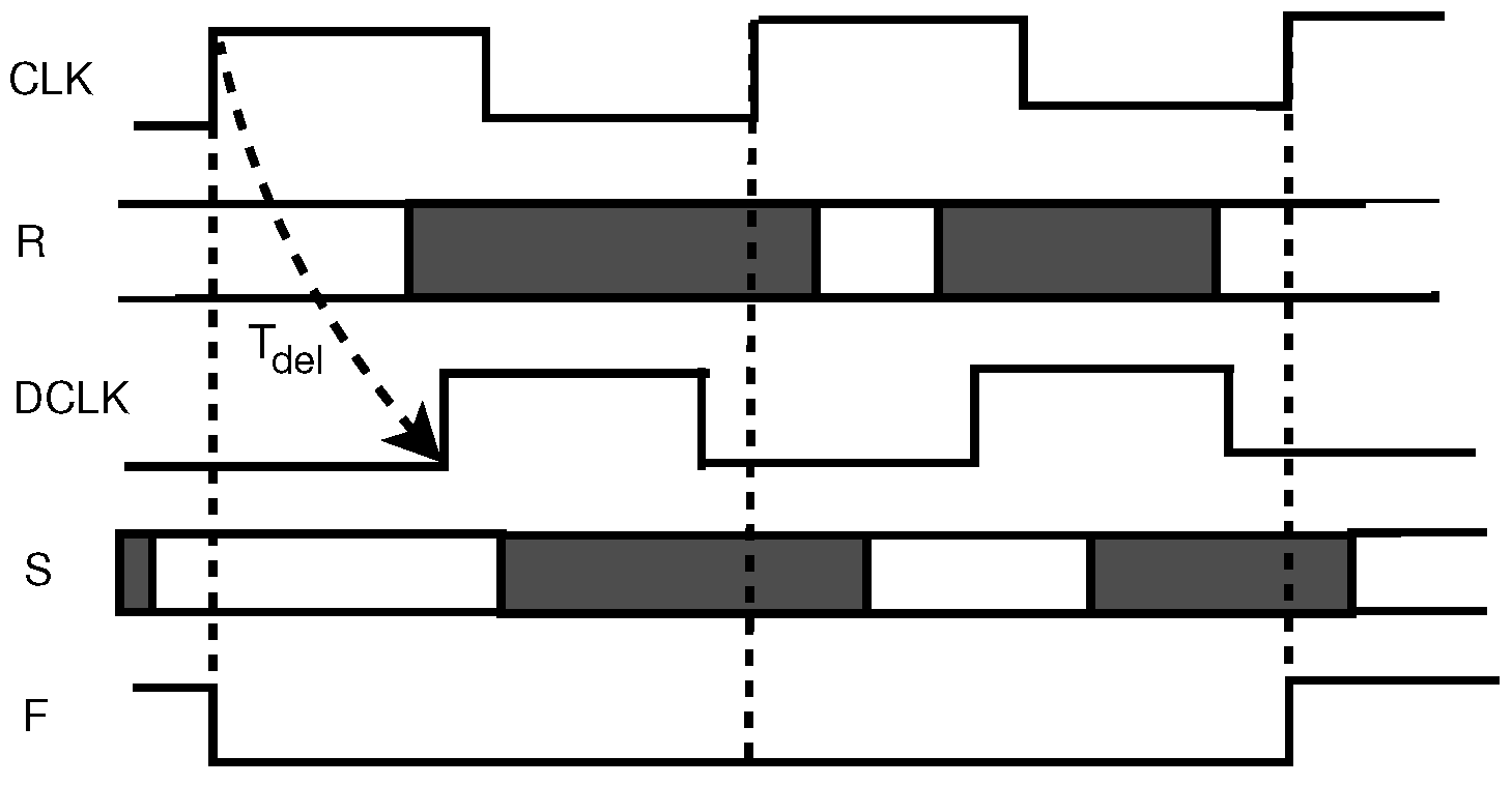
$Razor$ flipflop can be implemented in FPGA [6] by inserting a shadow flipflop running on a delayed clock. It is assumed that a circuit register (R) is lying at the end of one or more timing paths originating from any of the source registers. The shadow register (S) samples the same data as R but on a delayed clock ($DCLK$) that is lagged by $T_{del}$ from the main clock ($CLK$). Any data that arrive after R samples but before S samples will cause a discrepancy between the two registers, which is detected by the error flag (F). This $Razor$ flipflop is placed in each MAC unit of our systolic array. The multiplication and addition process in each MAC of our design is computed using the rising edges of $CLK$ and $DLK$. The $CLK$-driven output of the multiplication and addition process of each MAC is stored in the R register. The $DCLK$-driven output of the multiplication and addition process of each MAC is stored in the shadow register (S). The inclusion of $Razor$ doubles the number of multipliers and adders required for the systolic array, but it can detect whether runtime failure occurred in MACs due to the near-threshold biasing voltage. The timing diagram of the $Razor$ is shown in Figure 5.

Figure 5. Timing diagram of fault detection.

3. Hybrid Configuration: Static and Runtime Schemes

To mitigate timing failure issues in the critical voltage region, we adopt two sequential schemes. (i) The static scheme involves FPGA partitioning and rough $V_{ccin{t}_i}$ estimation depending on the FPGA technology. (ii) The runtime scheme is divided into two separate processes, namely timing error correction to calibrate the suitable $V_{ccin{t}_i}$ for each partition of FPGA using $Razor$ flipflop and (B) timing error correction and prediction based on heuristics for determination of input sequence family [5] and calibration of the suitable $V_{ccin{t}_i}$. Each partition of FPGA consists of a group of MACs. All the groups of MACs form a systolic array of the TPU. Apart from the systolic array, the TPU has memory to store active and weight inputs, the PCI interface, controlling circuitry, etc.

3.1. Static Scheme

The proposed static scheme operates within the $Vivado$/$VTR$ and $Python$ environments when the TPU is offline. As shown in Figure 1, synthesis is the first step of the proposed tool flow, which takes a netlist of complex logic blocks (CLBs) of the systolic array generated by the $Vivado$ or $VTR$ tool. This netlist from the synthesis report is generated after technology mapping and packing stages, which contain time slacks of all the possible paths of the systolic array. The proposed approach considers only nodes along paths because (i) the nodes along the path have data dependencies, which should be placed in the same FPGA partition even without considering the voltage scaling [20]. (ii) The slack values of the nodes along paths are usually close to each other. The second step of the proposed methodology involves the choice of the clustering algorithm and cluster generation. As stated in Section 4, the four clustering algorithms, namely the hierarchy, K-means, mean-shift and DBSCAN algorithms, create multiple clusters of MACs with the paths available in the synthesis report. Even for the same number of clusters, different algorithms classify the data points slightly differently.

The primary concern is to identify clusters of MACs that can share the minimum slacks available across the other MACs. Even for the same number of clusters, different algorithms classify the data points slightly differently. Unlike the K-means algorithm, the hierarchical, mean-shift and DBSCAN algorithms do not need the number of clusters to be specified beforehand. DBSCAN is found to perform the best in this case, as it groups together nearby data points, has a reasonable time complexity and can also identify outliers. Hence, clustered paths returned by DBSCAN are chosen for subsequent processes.

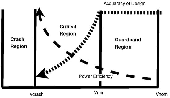
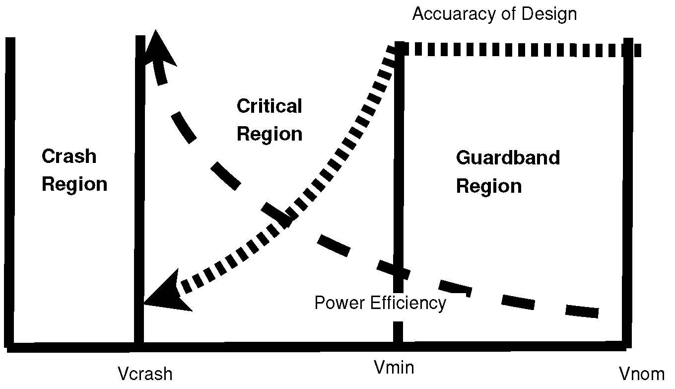
Once the number of clusters is fixed, we need to decide the voltage values of different FPGA partitions. In Figure 6, we illustrate three voltage regions in an FPGA, which are also supported by the research work reported in [4]. A voltage below the FPGA crashing voltage ($V_{crash}$) causes timing failure, which reduces the DNN accuracy to near zero. The region between minimum voltage ($V_{min}$) and nominal voltage ($V_{nom}$) is called the guard-band region, where the DNN accuracy is 100% but power efficiency is the least. In the critical region, the closer the voltage is to $V_{crash}$, the higher the power efficiency and the lower the DNN accuracy. Similarly, if $V_{ccint}$ is closer to $V_{min}$ in the critical region, the power efficiency decreases and DNN accuracy increases. In our proposed architecture, we assume the operating voltage range for the systolic array is $V_{crash}$ to $V_{min}$. If we have P clusters computed by the chosen clustering algorithm, we need P partitions in FPGA. The primary $V_{ccint}$ estimation for each FPGA partition is computed by Algorithm 1. In Xilinx FPGA, the coordinates of circuit components are specified by two slice parameters $(X_i,Y_j)$. Each FPGA partition has a range within these coordinates. The clustered MACs are placed in the same FPGA partition by mentioning the slice parameters $(X_i,Y_j)$.

Figure 6. Voltage behavior for $V_{ccint}$.

In the third step of the proposed methodology, each clustered path computed by the clustering algorithms is placed in a particular FPGA partition, which is restricted by specific $X_i,Y_j$ ranges. This restriction is applied to the xdc file during the $Generate$ $Constraint$ $File$ process.

Algorithm 1 Static Voltage Scaling

Require: $V_{ccint}$, $V_{min}$, $V_{crash}$ & P      1: $V_s$=$\frac{V_{min}-V_{crash}}{P}$      2: $V_l=V_{crash}$      3: for i = 1 to P do      4:    $V_{ccin{t}_i}$ = $\frac{V_l+V_l+V_s}{2}$      5:    $V_l=V_l+V_s$      6: end for

The rough $V_{ccint}$ calculation is performed by the static voltage scaling algorithm shown in Algorithm 1, which calculates a stepping voltage ($V_s$) from $V_{min}$ and $V_{crash}$. Thereafter, the $V_{ccin{t}_i}$ of the ith partition is calculated based on the stepping voltage ($V_s$). The static voltage scaling algorithm distributes $V_{ccint}$.

3.2. Runtime Scheme

Runtime scheme is divided into two processes.

3.2.1. Runtime Error Correction (REC)

The $V_{ccin{t}_i}$ of the ith FPGA partition calculated by Algorithm 1 is calibrated to the $V_{ccin{t}_i}$ pin of the ith FPGA partition. The calculation of $V_{ccin{t}_i}$ by Algorithm 1 is based on the number of partitions (P) and the critical voltage region ($V_{min}-V_{crash}$), which solely depends on the type of FPGA technology. However, the appropriate $V_{ccin{t}_i}$ of the ith FPGA partition should also depend on the minimum slack values of MACs of that partition. The static strategy calculates a rough estimation of $V_{ccin{t}_i}$, whereas the runtime strategy calibrates $V_{ccin{t}_i}$ according to the runtime timing failure of the systolic array. In the runtime scheme, we use one of the most popular runtime timing error detection schemes, $Razor$, which uses double-sampling flipflop to detect timing violations of pipeline stages. The $Razor$ flipflops are connected with every MAC of the systolic array to indicate timing failure. Each MAC has a timing failure flag, which is controlled by the $Razor$ flipflop. If any timing failure flag of any MAC placed in the ith FPGA partition is high, the $V_{ccin{t}_i}$ of that ith FPGA partition is increased by one step. If all the timing failure flags of all MACs placed in the ith FPGA partition are low, the $V_{ccin{t}_i}$ of that ith FPGA partition is decreased by one step. Before starting the actual run of the proposed systolic array, if we have a trial run, all the $V_{ccin{t}_i}$ of all partitions are tuned accurately by this $runtime$ process. The voltage-boosting circuit inside the VCU can be implemented externally following the technique proposed in [21].

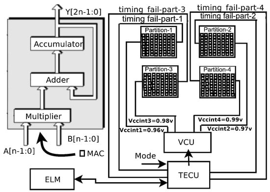
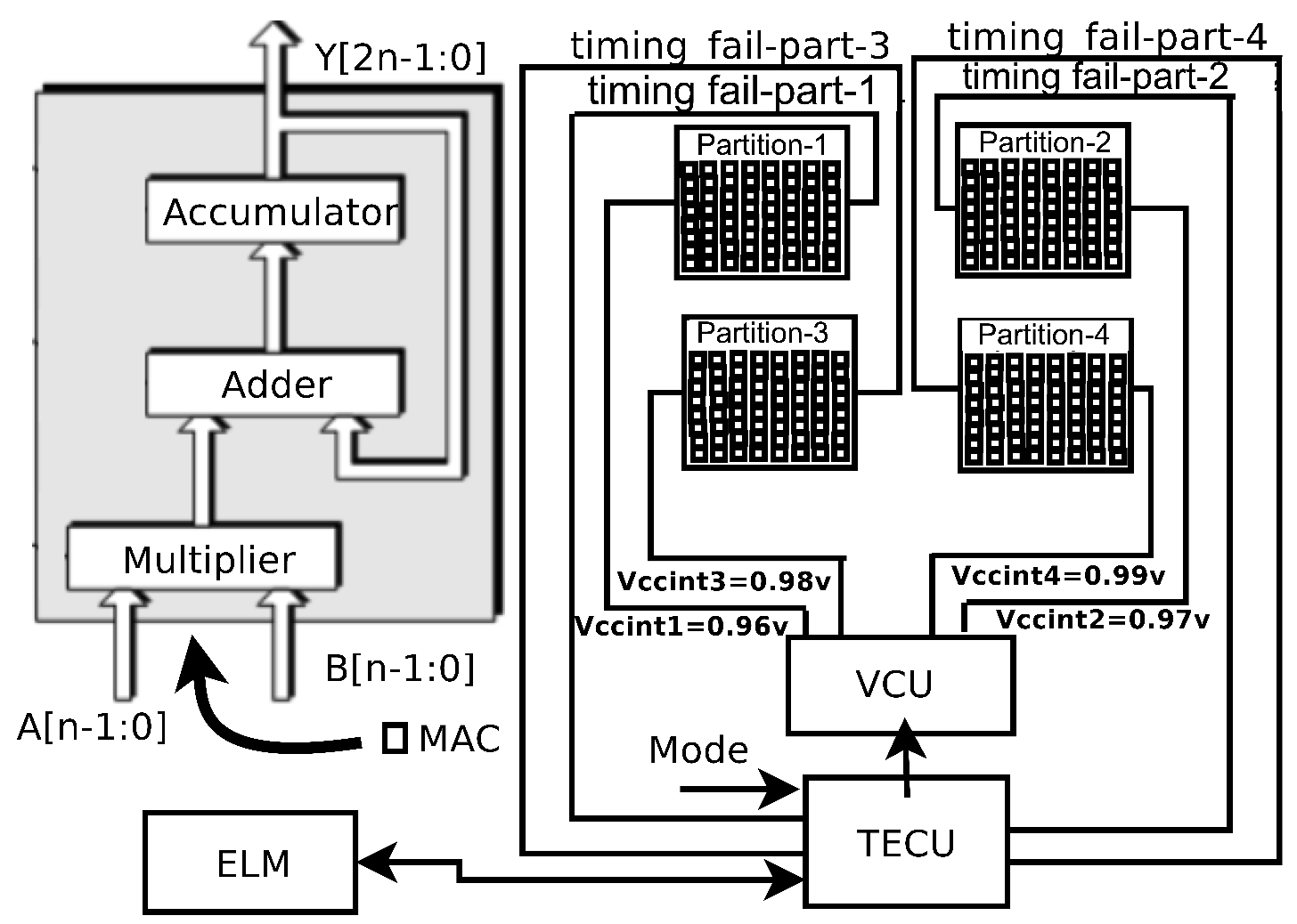
In Figure 7, we show that the cluster algorithm partitions the FPGA into four islands. The static scheme described in Section 3.1 calculates four $V_{ccin{t}_i}$ values, namely $V_{ccin{t}_1}$,$V_{ccin{t}_2}$, $V_{ccin{t}_3}$ and $V_{ccin{t}_4}$, for FPGA partition-1, partition-2, partition-3 and partition-4, respectively. The Voltage Control Unit (VCU) distributes $V_{ccin{t}_i}$ values, namely $V_{ccin{t}_1}$, $V_{ccin{t}_2}$, $V_{ccin{t}_3}$ and $V_{ccin{t}_4}$ to FPGA partition-1, partition-2, partition-3 and partition-4, respectively. Thereafter, the TPU circuit can be on, and the runtime scheme becomes functional. In the first step of the runtime scheme, as shown in Figure 7, four FPGA partitions, namely partition-1, partition-2, partition-3 and partition-4, have four flags form $Razor$ flipflops, namely $timing\_fail\text{-}part\text{-}1$, $timing\_fail\text{-}part\text{-}2$, $timing\_fail\text{-}part\text{-}3$ and $timing\_fail\text{-}part\text{-}4$, respectively, to detect the timing failure of the available partition of the FPGA. Each $timing\_fail\text{-}part\text{-}i$ flag is the ANDed value of all error detection flags of all MACs placed in the ith partition. As shown in Algorithm 2, if the ith timing failure flag from the ith FPGA partition becomes high, the VCU steps up the $V_{ccin{t}_i}$ of that partition by $V_s$; otherwise, $V_{ccin{t}_i}$ is stepped down by $V_s$. The $mode$ input of timing error control unit (TECU) for the entire first step of the runtime scheme is logic ‘0’.

Algorithm 2 Runtime Voltage Scaling

Require:  $V_{ccint}$, $V_s$      1: for i = 1 to P do      2:    if $timing\_fail\text{-}part\text{-}i==1$ then      3:      $V_{ccin{t}_i}$ = $V_{ccin{t}_i}+V_s$      4:    else      5:      $V_{ccin{t}_i}$ = $V_{ccin{t}_i}-V_s$      6:    end if      7: end for

Figure 7. Example: partitioned FPGA; n = 4.

3.2.2. Runtime Error Prediction and Correction (REPC)

This process predicts timing error based on heuristics to determine the input sequence family. Apart from $V_{ccint}$, timing error also depends on the fluctuation of input sequences. It is noticed that input sequences that have similar delay characteristics can be grouped into the same family. The sequence of inputs from a family may have similar bit flips, which can cause similar delays. This paper adopts the algorithm from [5], which creates groups of input sequences with similar delays. Instead of storing each input sequence as a separate entry in memory, the algorithm proposed in [5] stores a single entry for input sequences wiht similar delays. These input sequences that cause similar delays are considered a group or family. This solution makes it hardware-efficient. In the second step of the runtime scheme, the $mode$ input is made to logic ‘1’, which indicates that the TECU is active for timing error prediction.

Algorithm 3 correlates different input sequences and delays and makes some groups or families. It divides the changes in bits of an input sequence into three different families, namely (i) dynamic bit positions, which have the highest president; (ii) static bit positions, which are not flipped; and (iii) insignificant bit positions, which are flipped but insignificant in terms of causing delay. Therefore, one input sequence can represent a group of input sequences that produce a similar delay. We designed FPGA-based dedicated hardware for Algorithm 2 proposed in article [5]. When $Razor$ indicates the timing error, lines 1 to line 4 of Algorithm 3 store the XORed value of the current active(s) ($cur\_active$) and previous active(s) ($prev\_active$) in the Error Logic Memory (ELM), along with the coordinate(s) of any erroneous MAC(s). In line 6 of Algorithm 3, $new\_pat$ stores the XORed value of $cur\_active$ and $prev\_active$, while $new\_pat$ stores the dynamic bit position. In line 8, $similar$ stores the domination of dynamic bit positions, which contributes to delay characteristics. In line 9 and line 10, $num\_zero\_saved\_patt$ and $num\_zero\_similar$ count the number of zeros in the specific saved pattern of the ELM and the number of zeros in similar, respectively. If $num\_zero\_similar$ is greater than $num\_zero\_saved\_patt$, the specific $cur\_active$ and $prev\_active$ can cause error. This situation is termed as $MatchFound$, as stated in line 12. $MatchFound$ signifies that $new\_pat$ has a similar delay to that of the particular $saved\_patt$ stored in the ELM. Thereafter, the corresponding coordinate(s) of any MAC(s) stored in the ELM for the matched $saved\_patt$ is (are) sent to the voltage control unit (VCU). The VCU increases the voltage(s) of any particular FPGA partition(s) where an erroneous MAC(s) is (are) placed. This voltage control unit is similar to the voltage control unit (VCU) described in [5]. We designed a TECU for Algorithm 3. The ELM is mounted inside the TECU. The resource usage of the TECU unit for various sizes of systolic array is shown in Table 2.

Algorithm 3 Pattern Storing/Matching Heuristic

1: Store ELM(cur_active, prev_active){   2: xor_pat=cur_active xor prev_active   3: Store xor_pat   4: }   5: MATCH(cur_active, prev_active){   6: new_pat=cur_active xor prev_active   7: for all saved_patt do   8:    similar= new_pat or saved_patt   9:    num_zero_saved_patt=number of reset bits in saved_patt 10:    num_zero_similar=number of reset bits in similar 11:    if num_zero_similar>num_zero_saved_patt then 12:      match found 13:    end if 14: end for 15: }

Table 2. Overhead of timing error control unit.

Dimension of Systolic Array	Systolic Array		TECU
			ELM Size = 32		ELM Size = 64		ELM Size = 128		ELM Size = 256
	LUT	FF	LUT	FF	LUT	FF	LUT	FF	LUT	FF
16 × 16	4892	3040	866	404	858	455	949	477	1254	603
32 × 32	19,563	12,163	2256	404	2346	455	2570	477	2982	603
64 × 64	34,234	21,282	3631	404	3836	455	4189	477	4711	603

4. Clustering Algorithms

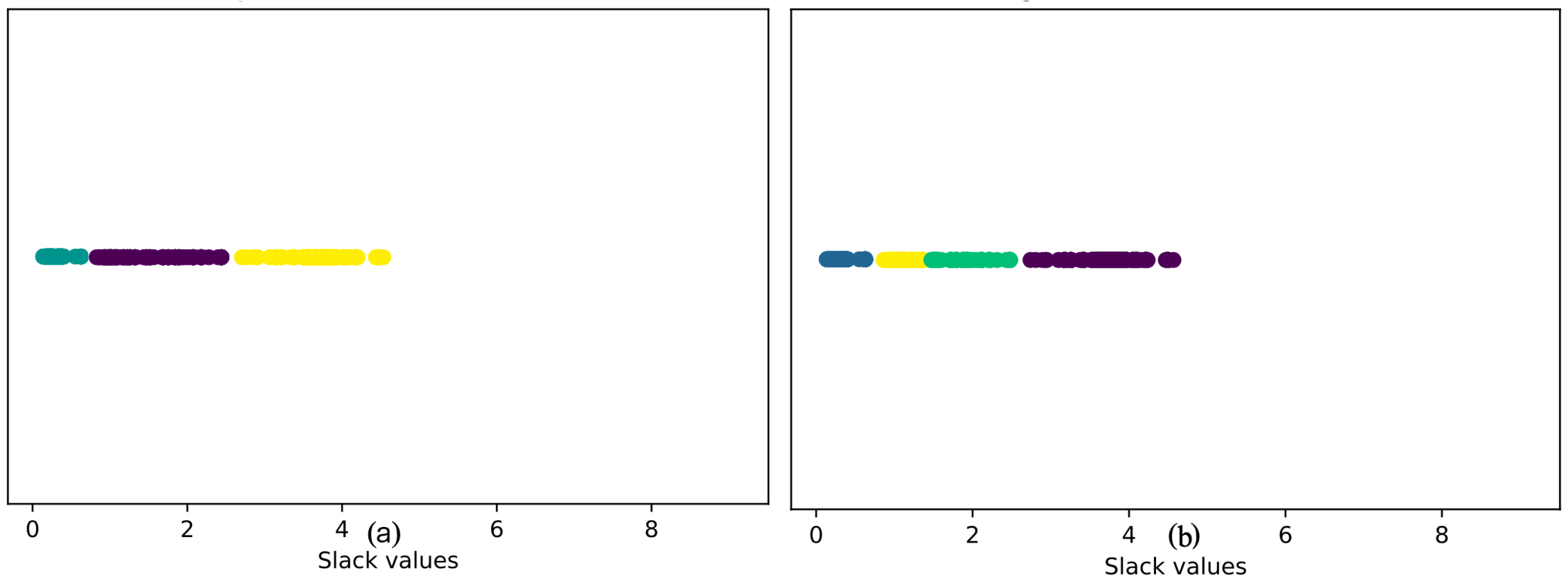
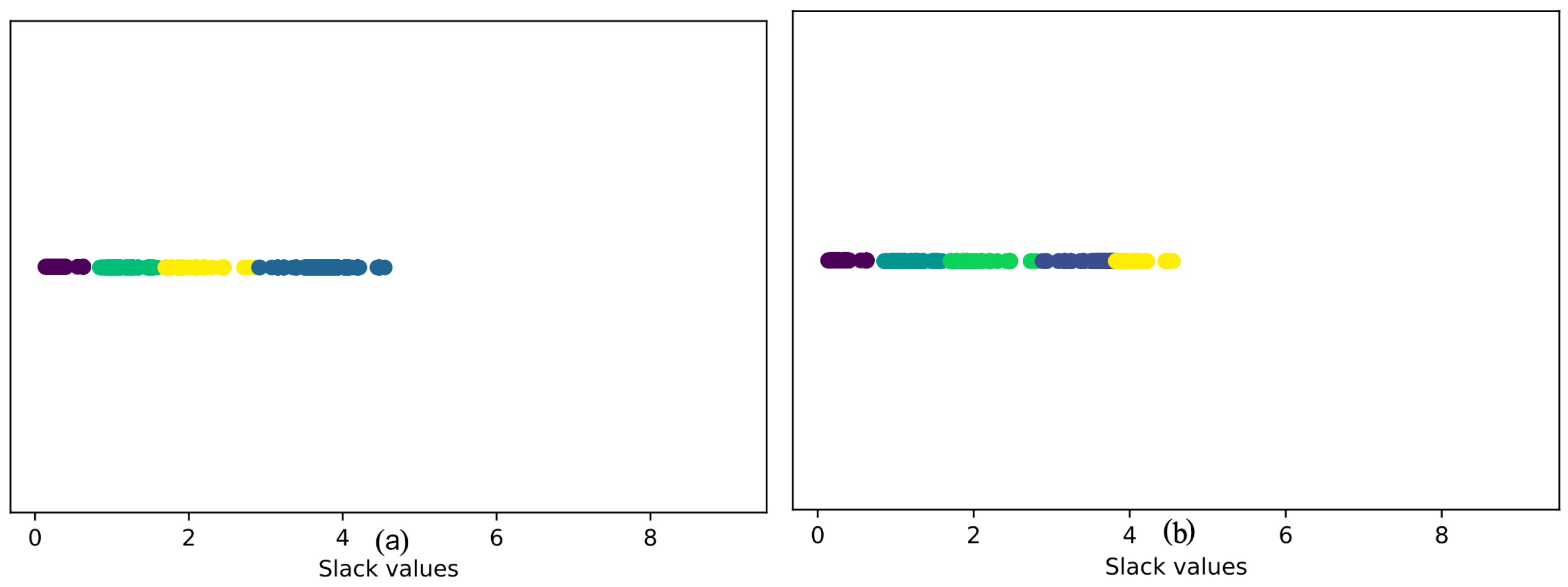
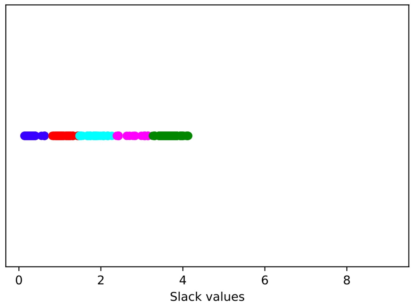
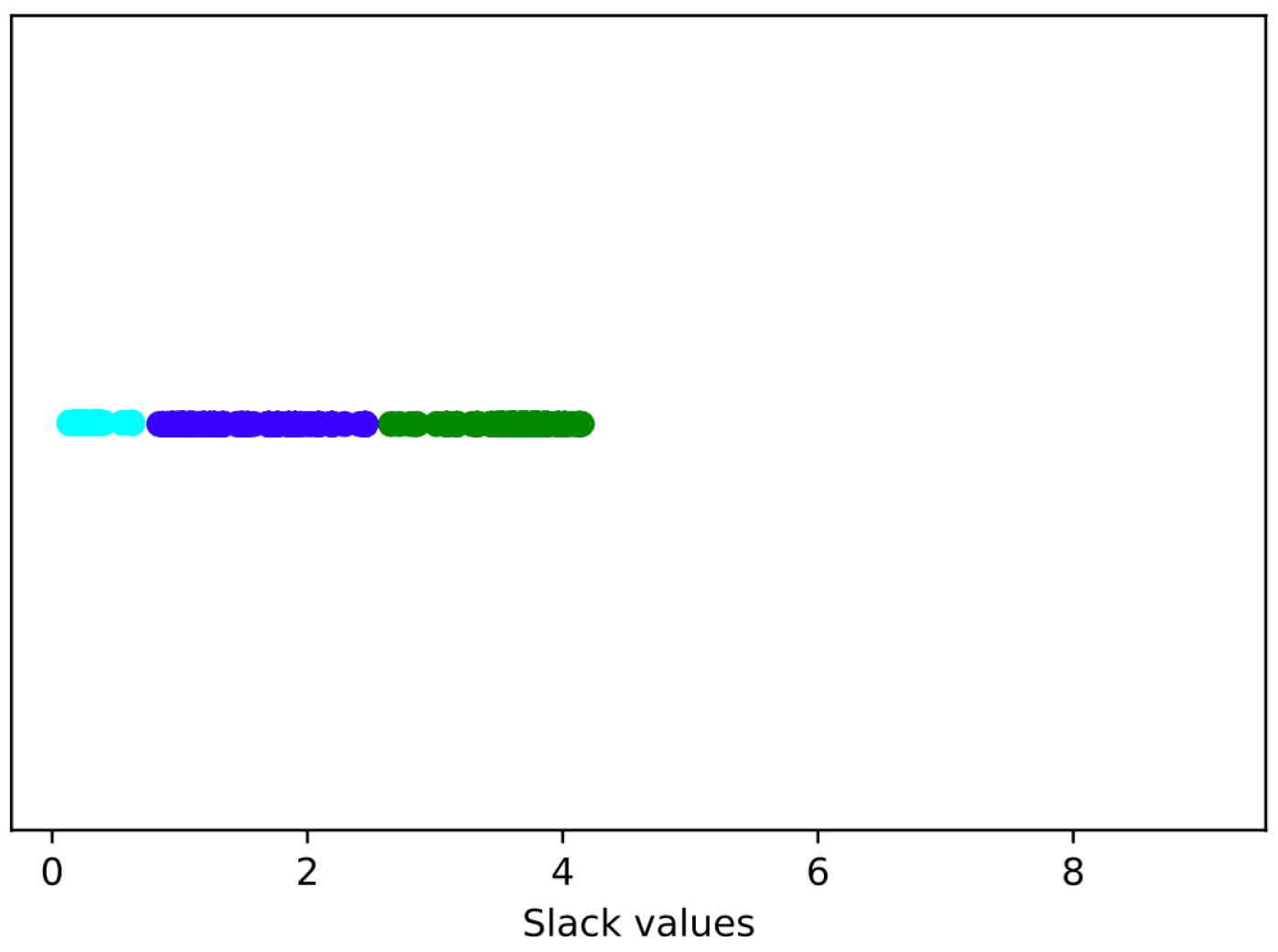
We investigated four clustering algorithms to group the MACs with similar minimum slacks. Algorithms can be chosen based on the design requirements if we want to set a predefined number of clusters or set hyperparameters to automatically determine the number of clusters. Different algorithms work well for different data distributions. The hierarchical, K-means, mean-shift and DBSCAN cluster algorithms create varying numbers of clusters, as shown in Figure 8, Figure 9, Figure 10 and Figure 11, respectively. Different colors represent different clusters, while the x-axis represents the minimum slack values of different MACs of the $16\times 16$ systolic array. Depending on our design requirements, we choose among the following four algorithms:

4.1. Hierarchical

The hierarchical clustering [22] algorithm considers each data point as a single cluster and measures the distance between two clusters based on a chosen distance measure (in this case, Euclidean distance). The two clusters that are closest to each other are merged. The process is continued until all clusters have been merged into a single cluster (root of the dendrogram). A dendrogram is a tree-like structure used for visualization the hierarchy of clusters. The number of clusters can be decided from the dendrogram. The hierarchical algorithm is computationally expensive for large datasets, having a time complexity of $O\left(n^3\right)$, where n is the number of data points. As is evident from the dendrogram, the length of the branch joining the last two clusters is the highest, indicating they are the most dissimilar, followed by the third and fourth clusters. The result of classifying the MACs based on their minimum slack values into three and four clusters is illustrated in Figure 8a and Figure 8b, respectively.

Figure 8. Hierarchical cluster of the slacks of a $16\times 16$ systolic array: (a) #clusters = 3; (b) #clusters = 4.

Figure 8. Hierarchical cluster of the slacks of a $16\times 16$ systolic array: (a) #clusters = 3; (b) #clusters = 4.

4.2. K-Means Clustering

K-means clustering can cluster data into a predefined number of groups (k). At the beginning, k cluster centers are randomly initialized [23]. The algorithm computes the distance between each data point and the cluster centers and assigns data points to the cluster whose center is closest. The cluster centers are then recomputed as the mean of the data points belonging to that cluster. The process is repeated for a predefined number of steps or until cluster centers do not change significantly. K-means clustering is simple and fast, and its time complexity is $O\left(n\right)$. Figure 9 illustrates the results of applying the K-means clustering algorithm to the minimum slack values of a $16\times 16$ systolic array (256 MACs) for four and five clusters.

Figure 9. K-means cluster of the slacks of a $16\times 16$ systolic array: (a) #clusters = 4; (b) #clusters = 5.

Figure 9. K-means cluster of the slacks of a $16\times 16$ systolic array: (a) #clusters = 4; (b) #clusters = 5.

4.3. Mean-Shift Clustering

Mean-shift clustering [24] is based on the idea of Kernel Density Estimation (KDE). KDE assumes that the data points are generated from an underlying distribution and tries to estimate the distribution by assigning a kernel to each data point. The most commonly used kernel is the Gaussian or RBF kernel. The mean-shift algorithm is designed in a way such that the points iteratively climb the KDE surface and are shifted to the nearest KDE peaks. It starts with a randomly selected point as the center of the RBF kernel. Thereafter, it proceeds by moving the kernel towards regions of higher density by shifting the center of the kernel to the mean of the points within the window (hence, the algorithm is termed mean-shift). This is continued until shifting the kernel no longer includes more points. This algorithm does not need the number of clusters to be specified beforehand, but it is computationally expensive compared to K-means (time complexity of $O(n\ast log(n\left)\right)$ in lower dimensions for Python $sklearn$ implementation). The selection of the window size/radius (r) can be non-trivial and plays a key role in the success of the algorithm. Setting the radius as 0.4 for the slack values of a $16\times 16$ systolic array yields five clusters, as observed in Figure 10.

Figure 10. Mean-shift clustering of the slacks of a $16\times 16$ systolic array.

Figure 10. Mean-shift clustering of the slacks of a $16\times 16$ systolic array.

4.4. DBSCAN

The DBSCAN algorithm has two important hyperparameters based on which it determines the number of clusters [25], namely epsilon, which is the maximum distance between two samples for one to be considered as in the neighborhood of the other, and minpoints, which is the number of samples in a neighborhood for a point to be considered as a core point. At each step, a data point that has not been visited before is taken. If there are more data points than $minpoints$ within its $epsilon$ radius, all the data points are marked as belonging to a cluster; otherwise, the first point is marked as noise. For all points in the newly formed cluster, points within their ‘epsilon’ neighborhood are checked and labeled as either belonging to a cluster or as noise. The process is continued until all data points have been labeled. The greatest advantage of DBSCAN is that it can identify outliers as noise, unlike other algorithms, which throw all points into a cluster even if one data point is significantly different from the rest. The time complexity of this algorithm is $O\left(n\right)$ for reasonable $epsilon$ values. This algorithm is not effective for clusters with varying density, since $epsilon$ and $minpoints$ are different for different clusters. Figure 11 illustrates how the DBSCAN algorithm creates three clusters of the MACs of a $16\times 16$ systolic array. Each of the three different colors represents a distinct cluster of MACs.

Figure 11. DB scan clustering of the slacks of a $16\times 16$ systolic array.

Figure 11. DB scan clustering of the slacks of a $16\times 16$ systolic array.

5. Implementation and Result

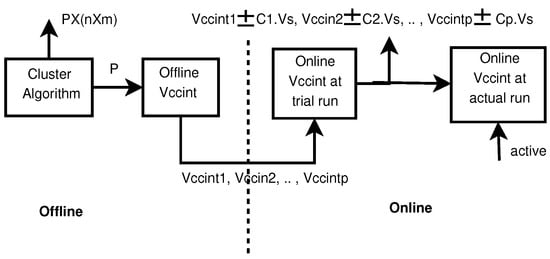
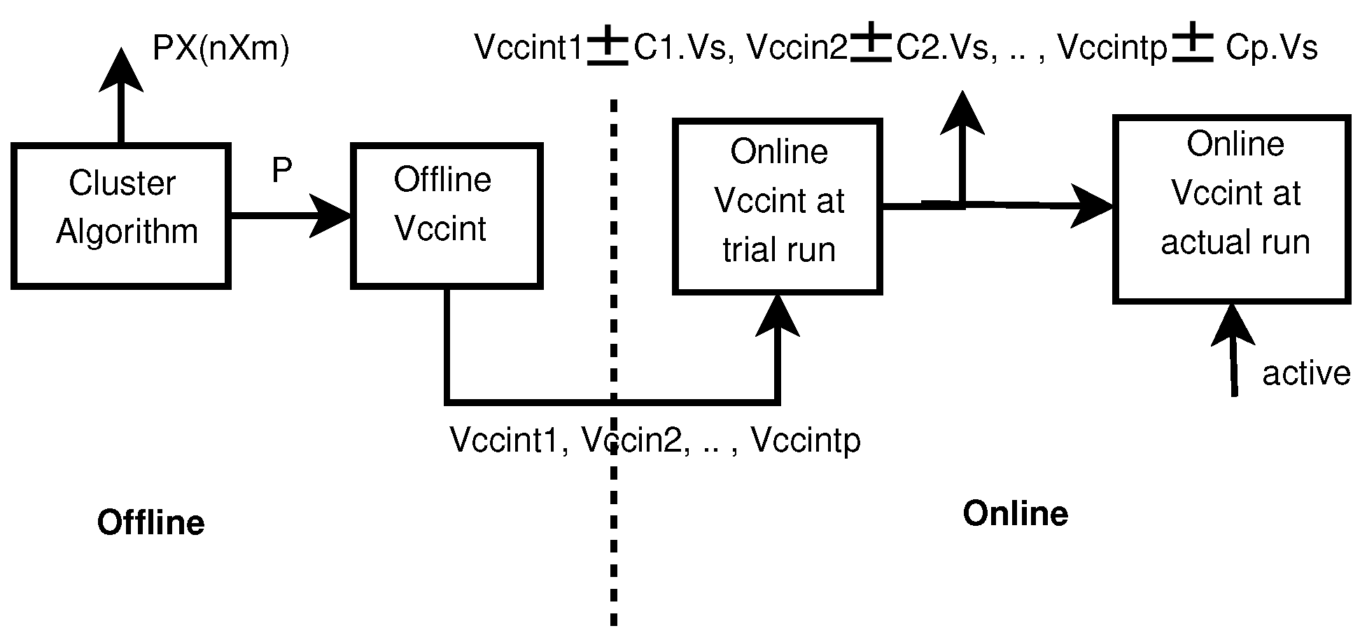
As mentioned in Section 2, the two proposed tool flows have two environments. The clustering algorithms for both $Vivado$ and $VTR$ are implemented in Python using the Scikit-learn library. The $synthesis$, $implementation$ and $bitfilegeneration$ of the $Vivado$ flow are performed by the board support package of the $Artix\text{-}7$ FPGA. The $synthesis$ and $implementation$ of the $VTR$ flow are performed by the board support package of 22 nm, 45 nm and 130 nm academic FPGAs. As shown in Figure 12, the cluster algorithm generates P partitions, and the dimensions of each partition are $(n\times m)$. The static scheme generates biasing voltages as follows:

$$P\times (n\times m)\{V_{ccin{t}_1},V_{ccin{t}_2},\dots ,V_{ccin{t}_i},\dots ,V_{ccin{t}_p}\}$$

(1)

for P partitions. The runtime scheme calibrates the biasing voltage according to the timing failure detected by $Razor$ placed in every MAC. The runtime scheme provides the following final set of biasing voltages:

$$\begin{array}{c}\hfill V_{ccin{t}_1}+C_1.V_s,V_{ccin{t}_2}+C_2.V_s,\dots ,V_{ccin{t}_i}+C_i.V_s,\dots ,\\ \hfill V_{ccin{t}_p}+C_P.V_s\end{array}$$

(2)

Here, $C_1$, $C_2$, … $C_p$ are integers starts from 0 to any positive value.

Figure 12. Flow diagram of the proposed framework.

5.1. Implementational Challenges

The proposed design could not be fully implemented, as none of the present-day FPGA devices support variable-voltage scaling in the different logic partitions. The implementation issues of a VCU with multiple $V_{ccint}$ values in different partitions are beyond the scope of our paper. However, we consider that the implementation of voltage scaling technology in ASICs [5] establishes the feasibility of implementation of voltage scaling technology in FPGAs.

5.2. Our Validation Strategy

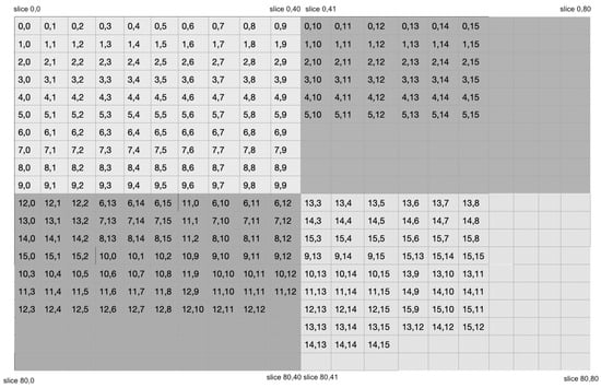
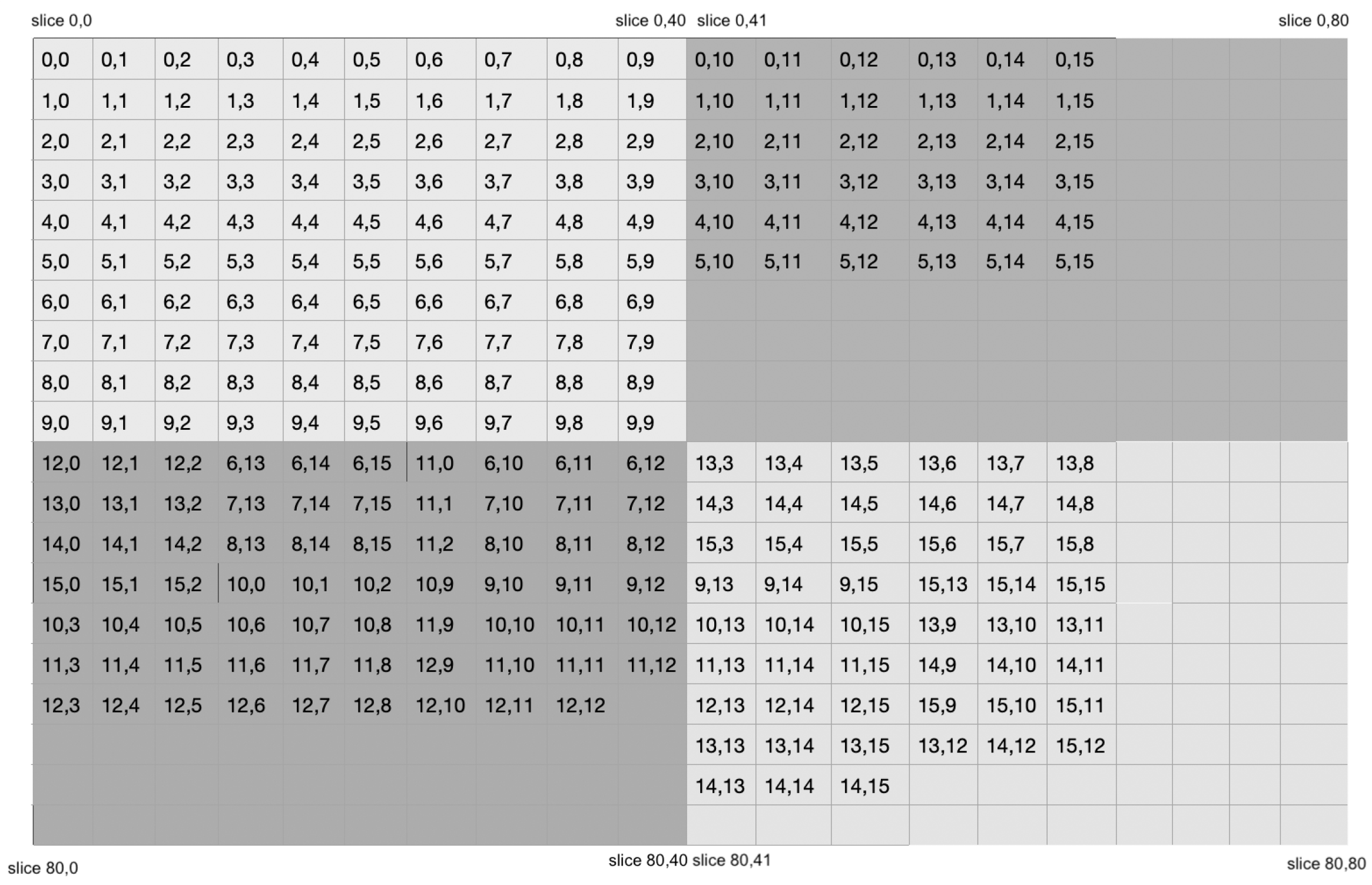
To validate the claim of the proposal, we implemented the proposed scheme using $Vivado$ and $VTR$ flows. We designed a systolic array with the following three different dimensions: $16\times 16$, $32\times 32$ and $64\times 64$. Let us take the example of a $16\times 16$ systolic array where $16\times 16=256$ MACs are placed in the FPGA. As shown in Figure 9b, the K-means clustering algorithm mentioned in Section 4 divides the $16\times 16$ systolic array into four partitions, namely $partition\text{-}1$, $partition\text{-}2$, $partition\text{-}3$ and $partition\text{-}4$, based on the silhouette coefficient. The sizes of the partitions are $partition\text{-}1$ = $10\times 10$ = 100, $partition\text{-}2$ = $6\times 6$ = 36, $partition\text{-}3$ = $3\times 23$ = 69 and $partition\text{-}4$ = $3\times 17$ = 51. As the current $Vivado$ tool does not allow the design to operated in the critical voltage region, our $16\times 16$ systolic array is tested in the guard-band region. Due to the unavailability of multiple $V_{ccint}$ supports in a single FPGA deviceat the same time, our design is implemented in one partition at a time. Therefore, the power measurement of the four partitions is also performed separately, where each partition is considered as an individual circuit. Due to the unavailability of multiple $V_{ccin{t}_i}$ values at a time in a single FPGA device, our runtime voltage calibration strategy is capable of scaling a single $V_{ccin{t}_i}$ for a partition. Current FPGAs do not have any voltage scaling standard. However, $Artix\text{-}7$ can perform voltage scaling by Inter-Integrated Circuit (I2C) command. Although $VTR$ allows the design to operated in critical regions, for the sake of a better comparative study, we have also use the same voltage ranges used in $Vivado$. The FPGA floor after clustering the MACs of the $16\times 16$ systolic array is depicted in Figure 13. Here, the coordinates are the row and column addresses of MACs in the systolic array.

Figure 13. FPGA Floor of 16 × 16 systolic array.

5.3. Results

This section studies how different sizes and architectures of systolic arrays, as well as parameters such as P, $V_{ccint}$ and $n\times m$, affect the proposed partition-based voltage-scaled architecture. It also compares the normalized performance of our architecture with that reported in [5]. The results of our implementations are based on three different sizes of systolic arrays, namely test 1, with a size of $16\times 16$; test 2, with a size of $32\times 32$; and test 3, with a size of $64\times 64$. All these tests are conducted using $Artix\text{-}7$ (D1), $VTR\text{-}22$ nm (D2), $VTR\text{-}45$ nm (D3) and $VTR\text{-}130$ nm (D4) FPGAs. Test 1 is also implemented with different variants of systolic arrays.

5.3.1. Different Sizes of Systolic Arrays

Table 3 shows the dynamic power consumption of $16\times 16$ (test 1), $32\times 32$ (test 2) and $64\times 64$ (test 3) systolic arrays with different sizes of partitions. The dynamic power measurements of $Vivado$ and $VTR$ implementations are carried out by a Xilinx $Vivado$ probe and $VTR$, respectively. The guard-band region for the $Artix\text{-}7$ FPGA in $Vivado$ implementations ranges from 0.95 volts to 1.00 volts. For test 1, the number of partitions is $P=4$, $V_{min}=V_{nom}=1.00volts$ and $V_{crash}=V_{min}=0.95volts$; therefore, $V_s=0.0125volts$. Algorithm 1 calculates the $V_{ccin{t}_i}$ of the four FPGA partitions of this design, which are $V_{ccin{t}_1}=0.956$ for $partition\text{-}1$, $V_{ccin{t}_2}=0.968$ for $partition\text{-}2$, $V_{ccin{t}_3}=0.985$ for $partition\text{-}3$ and $V_{ccin{t}_4}=0.993$ for $partition\text{-}4$. We observe that when the partial sums are moved to the bottom rows of the systolic array, the timing error increases significantly [5].

Table 3. Comparison of dynamic power (mw) for $Vivado$ and $VTR$ flows.

				Dynamic Power (mw)
25 °C Ambient Temperature and 100 MHz Clock	Size of Systolic Array	Partition No.	${\mathbf{V}}_{{\mathbf{ccint}}_{\mathbf{i}}}$ (Volts)	Vivado 28 nm Artix-7 (D1)	VTR 22 nm (D2)	VTR 45 nm (D3)	VTR 130 nm (D3)	Remarks
Without Voltage Scaling	$16\times 16$	NA	1.00	408	328	469	1808	D1, D2, D3 and D4 required
	$10\times 10$	partition-1	0.96	382	310	446	1753	1 stage K-Means clustering
Voltage	$6\times 6$	partition-2	0.97
Scaled	$3\times 23$	partition-3	0.98
	$3\times 17$	partition-4	0.99
Test:1 *: % of Dynamic Power Reduction				6.4	5.4	4.9	3.1
% of timing overhead of our tool flow				11	15	12	13
Without Voltage Scaling	$32\times 32$	NA	1.00	1538	1072	1549	6172	D1, D2, D3 and D4 required
Voltage Scaled	$18\times 16$	partition-1	0.96	1411	1001	1472	5956	1 stage K-Means clustering
	$18\times 18$	partition-2	0.97
	$6\times 6$	partition-3	0.98
	$16\times 17$	partition-4	0.99
	$8\times 13$	partition-5	1.00
Test:2 *: % of Dynamic Power Reduction				8.2	6.6	4.8	3.5
% of timing overhead of our tool flow				15	16	17	17
Without Voltage Scaling	$64\times 64$	NA	1.1	not supported	4127	6023	24,896	D2, D3 and D4 required 2 stages K-Means
Voltage Scaled	$43\times 16$	partition-1	0.7	Not Supported	3648	5402	22,716	clustering; D1 Not supported, $V_{ccint}$ < 0.95 NA in Artix-7
	$22\times 22$	partition-2	0.78
	$18\times 18$	partition-3	0.86
	$28\times 28$	partition-4	0.92
	$28\times 27$	partition-5	0.98
	$20\times 23$	partition-6	1.04
	$24\times 25$	partition-7	1.1
Test:3: % of Dynamic Power Reduction				-	11.6	10.3	8.7
% of timing overhead of our tool flow				-	29	28	30

* Lower bounds of improvement due to the constraint of $Vc{c}_{int}$.

As depicted in Figure 13, the K-means clustering algorithm is divides test 1, which consists of a $16\times 16$ systolic array, into four partitions. The top-left partition-1 consists of a $10\times 10$ systolic array that has $V_{ccin{t}_1}=0.956\approx 0.96$. Similarly, top-right partition-2 consists of a $6\times 6$ array with $V_{ccin{t}_2}=0.968\approx 0.97$, bottom-left partition-3 consists of a $3\times 23$ array and has $V_{ccin{t}_3}=0.985\approx 0.98$ and bottom-right partition-4 consists of a $3\times 17$ array and has $V_{ccin{t}_4}=0.993\approx 0.99$. As depicted in Table 3, the adoption of voltage scaling technology in the design of $test1$ reduces dynamic power consumption for $Vivado$ commercial FPGAs by 6.4% and reduces dynamic power for $VTR$ academic FPGAs of 22 nm, 45 nm and 130 nm by 5.4%, 4.9% and 3.1%, respectively. The design of $test2$ has five partitions, which reduces dynamic power for $Vivado$ by 8.2% and reduces dynamic power for $VTR$ from 6.6% to 3.5%. Finally, the design of $test3$ has seven partitions, which reduces dynamic power from 11.6% to 8.7% on the $VTR$ platform. Due to the limited range of biasing voltage in $Vivado$, test 1 and test 2 have lower bounds on improvements. In test 3, biasing voltage drops to closer to NTC for $VTR$. As expected, the power reduction increases substantially from 11.6% to 8.7%. It is observed that the percentage of dynamic power reduction is less for longer transistor channels. Table 3 demonstrates that among all the designs (D1, D2, D3 and D4) in test 1, test 2 and test 3, test 3-D2 ($VTR$ 22 nm FPGA) exhibits the highest reduction in dynamic power percentage compared to all other designs with NTC. This is because shorter channel lengths generally result in lower gate capacitance and faster switching speeds, which can reduce dynamic power consumption. The $Razor$ logic overhead costs 453 LUTs and 89 flipflops for a 16 × 16 systolic array.

5.3.2. Variants of Systolic Array Architecture

We have use the voltage scaling technique in four variants of systolic arrays, namely a One-Dimensional Systolic Array (1DSA0) [26], a Modified One-Dimensional Systolic Array (1DSA0) [27], a Two-Dimensional Systolic Array (2DSA) [28] and tree architecture [28]. As shown in Table 4, the adoption of voltage scaling in all these existing variants of systolic arrays reduces the dynamic power by 3.12% to 8.27%. Table 4 demonstrates that the proposed voltage scaling methodology not only reduces a significant amount of dynamic power consumption in TPU-based systolic arrays but that it may also be equally effective with one-dimensional systolic arrays, modified one-dimensional systolic arrays, two-dimensional systolic arrays and tree architectures.

Table 4. Power consumption of different of voltage-scaled systolic array architectures.

Tool	Size = 16 × 16, Temp—25 °C, Clock = 100 MGhz, # MAC = 256	Dynamic Power (mw)	% Dynamic Power Reduction	# Accessed Data	# Load Clock	# Idle Clock	# Working Clock	# Total Clock
Vivado-Artix7	1DSA0	489	6.14	1024	512	256	256	1024
	1DSA0-VS	459
VTR-22 nm	1DSA0	387	7.24
	1DSA0-VS	359
VTR-45 nm	1DSA0	502	5.17
	1DSA0-VS	476
VTR-130 nm	1DSA0	2251	4.35
	1DSA0-VS	2153
Vivado-Artix7	1DSA1	481	6.65	256	1024	240	256	752
	1DSA1-VS	449
VTR-22 nm	1DSA1	381	7.87
	1DSA1-VS	351
VTR-45 nm	1DSA1	496	5.24
	1DSA1-VS	470
VTR-130 nm	1DSA1	2242	3.92
	1DSA1-VS	2154
Vivado-Artix7	2DSA	509	6.87	8192	16	240	256	512
	2DSA-VS	474
VTR-22 nm	2DSA	411	8.27
	2DSA-VS	377
VTR-45 nm	2DSA	596	5.2
	2DSA-VS	565
VTR-130 nm	2DSA	2311	4.28
	2DSA-VS	2212
Vivado-Artix7	Tree	528	6.25	8192	16	240	256	512
	Tree-VS	495
VTR-22 nm	Tree	431	7.65
	Tree-VS	398
VTR-45 nm	Tree	613	5.22
	Tree-VS	581
VTR-130 nm	Tree	2423	4.29
	Tree-VS	2319
Vivado-Artix7	Proposed TPU SA	408	6.37	1024	16	0	256	272
	Proposed TPU SA-VS	382
VTR-22 nm	Proposed TPU SA	328	5.8
	Proposed TPU SA-VS	310
VTR-45 nm	Proposed TPU SA	469	5.15
	Proposed TPU SA-VS	446
VTR-130 nm	Proposed TPU SA	1808	3.13
	Proposed TPU SA-VS	1753

5.3.3. Effects of P, $V_{ccint}$ and $n\times m$ in Dynamic Power

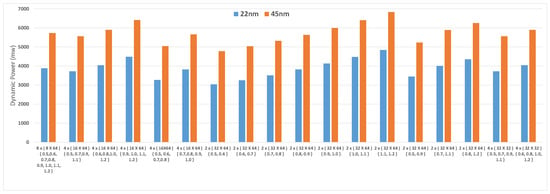
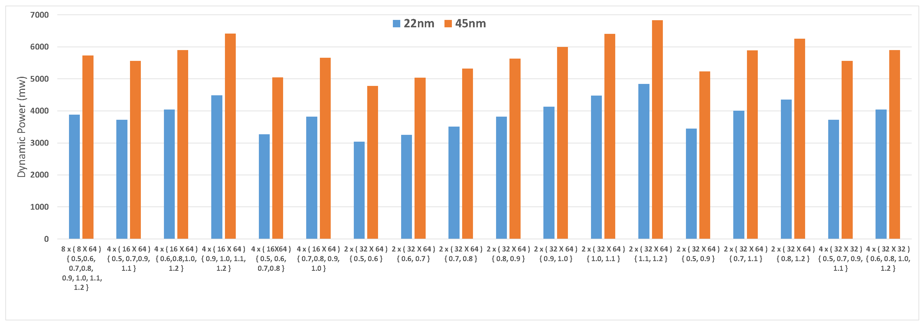
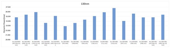
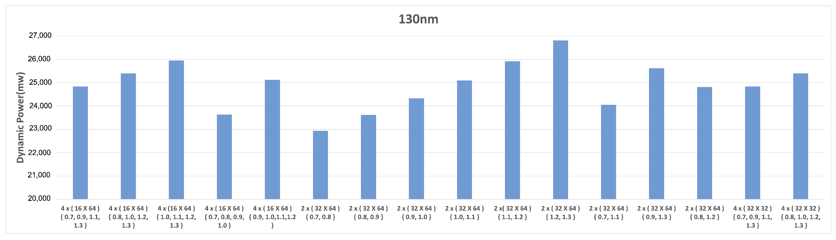
In Figure 14 and Figure 15, we show the dynamic power consumption of different variants of 64 × 64 systolic arrays on 22 nm, 45 nm and 130 nm academic FPGAs using the $VTR$ flow. Figure 14 and Figure 15 show that variation of three parameters, such as the number of partitions (P), the biasing voltage ($V_{ccin{t}_i}$) of each partition and the dimensions of each FPGA partition ($n\times m$) changes the dynamic power consumption of 64 × 64 systolic arrays by 18%, 21% and 39% for 22 nm, 45 nm and 130 nm academic FPGAs, respectively. Here, the number of clusters or partitions (P) and the dimensions of each partition ($n\times m$) are calculated by cluster algorithms. The biasing voltage ($V_{ccin{t}_i}$) of each FPGA partition is roughly calculated by a static scheme, and further calibration of accurate $V_{ccin{t}_i}$ is performed by the runtime scheme. Such significant effects of P, $n\times m$ and $V_{ccin{t}_i}$ on dynamic power consumption show that the cluster algorithm and the static and runtime schemes are very crucial steps of proposed framework. As an example, in Figure 14 and Figure 15, the name of one variant of the systolic array is $4\times (32\times 32)\{0.8,1.0,1.2,1.3\}$ (the rightmost bar in Figure 15), where P = 4, $n\times m$ = $32\times 32$ and the biasing voltages of the four partitions are 0.8 volts, 1.0 volts, 1.2 volts and 1.3 volts. In Figure 14 and Figure 15, the $V_{ccin{t}_i}$ for 130 nm varies the threshold voltage from 0.7 volts to 1.3 volts, whereas for 22 nm and 45 nm, $V_{ccin{t}_i}$ varies from 0.5 volts to 1.2 volts. Although the threshold voltage of 45 nm is 0.5 volts and for 22 nm, it is 0.45 volts, for comparative purposes, in both cases, we measure it form 0.5 volts. It is known that the dynamic power reduces by the square of the supply voltage ($V_{ccin{t}_i}$). Also, the $2\times (32\times 64)\{0.5,0.6\}$ variant of the systolic array implemented in 22 nm and 45 nm technology has the maximum number of MACs running with minimum $V_{ccin{t}_i}$ values as compared to other reported variants, as shown in Figure 14. Thus, the aforementioned variant consumes minimum dynamic power as compared to other variants reported in Figure 14. Going by the same reasoning, the $2\times (32\times 64)\{0.7,0.8\}$ variant in 135 nm technology consumes minimum dynamic power when compared to the other variants, as reported in Figure 15. The minimum voltage step of the power supply [21] is considered as 0.1 volt. We observe that the timing reports of 16 × 16 and 32 × 32 systolic arrays before partitioning and after partitioning show very insignificant effects on delay in wires, as well as placement and routing difficulties. Hence, the reclustering process is not required for the aforementioned systolic arrays. However, for 64×64 systolic arrays, delays of design paths vary. Therefore, a reclustering (second stage) process is required.

Figure 14. Comparison of dynamic power (mw) of various variants of 64 × 64 systolic arrays on 22 nm and 45 nm.

Figure 15. Comparison of dynamic power (mw) of various variants of 64 × 64 systolic arrays on 130 nm.

5.3.4. Normalized Performance

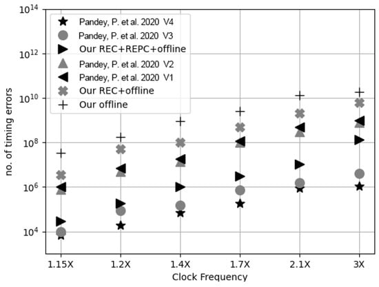
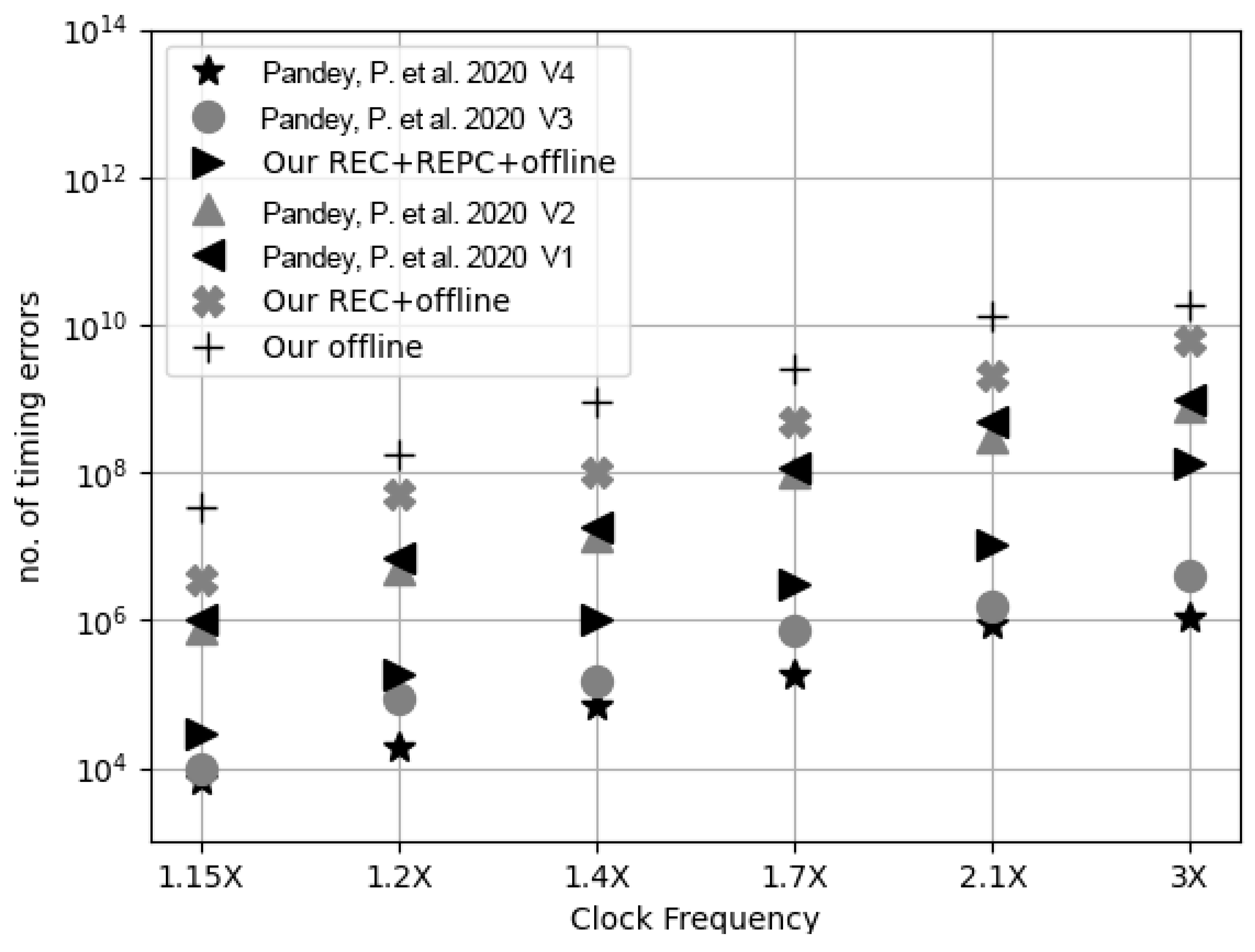
Figure 16 shows that the number of timing errors increases with the clock frequency of the design. The normalized performance of our proposed 256 × 256 systolic array is compared with the four variants designed in [5]. We designed three variants of systolic arrays, namely (i) a systolic array with a prediction model described in Section 3.2.2 in which the ELM size is 10 (REC + REPC + offline), (ii) a systolic array without a prediction (REC + offline) model and (iii) a systolic array with offline calibration only. In [5], V1 incorporates TE-Drop error correction, while V2 does not include a prediction model. V3 is a lighter variant with only one error-causing pattern in the ELM, whereas the V4 is a variant with 10 error-causing patterns in the ELM. In Figure 16, it is noticed that our 28 nm FPGA-based systolic array faces more timing errors compared to the 15 nm ASIC-based implementation reported in [5]. The configurable switches and longer channel lengths of the transistors used in FPGAs cause more delays, which affect timing error significantly. As shown in Table 3, the timing overhead of the proposed CAD flow is insignificant. The proposed CAD flow is executed on an Intel $i5$, Linux, 8GB RAM platform. A comparison of CIFAR-10 benchmarks with the results of [5] is shown in Table 5.

Figure 16. Normalized Performance [5].

Table 5. Comparison of benchmarks with [5].

Ref.	Model	Dataset	Input Size	Output Size	# Layers	Accuracy
Our	Goggle Net	Cifar-10	32 × 32	32 × 32	6	84%
	VGG Net	Cifar-10	32 × 32	32 × 32	6	89%
[5]	Goggle Net	Cifar-10	NR *	NR *	NR *	77%

* NR = Not Reported.

6. Conclusions

This paper proposes a systolic array where the MACs are placed in different partitions of FPGAs based on the minimum slacks of different MACs. Each partition of the FPGA uses a different biasing voltage ($V_{ccint}$). The proposed $runtime$ and $static$ schemes can tune appropriate $V_{ccint}$ values, MACs with similar minimum slacks placed in the same partitions. The proposed error correction and prediction mechanism, utilizing Razor flipflops and a matching heuristic algorithm, effectively addresses timing failures resulting from lower $V_{ccint}$ levels that are close to NTC. The experimental results demonstrate that a voltage-scaled systolic array can significantly reduce power consumption. The proposed technique does not affect the logic of design paths. Therefore, this method can be applied to any existing low-power neural network architecture to reduce additional power consumption. Similarly, partition-based voltage scaling can be utilized for other high-performance hardware accelerators to decrease power consumption. In our future efforts, we will explore the development of an automated tool flow to enable near-threshold computation for diverse high-processing algorithms, with the aim of minimizing power consumption.

References

- Kimm, H.; Paik, I.; Kimm, H. Performance Comparision of TPU, GPU, CPU on Google Colaboratory Over Distributed Deep Learning. In Proceedings of the 2021 IEEE 14th International Symposium on Embedded Multicore/Many-Core Systems-on-Chip (MCSoC), Singapore, 20–23 December 2021; pp. 312–319. [Google Scholar] [CrossRef] [Scilit]
- Caulfield, A.M.; Chung, E.S.; Putnam, A.; Angepat, H.; Fowers, J.; Haselman, M.; Heil, S.; Humphrey, M.; Kaur, P.; Kim, J.Y.; et al. A cloud-scale acceleration architecture. In Proceedings of the 2016 49th Annual IEEE/ACM International Symposium on Microarchitecture (MICRO), Taipei, Taiwan, 15–19 October 2016; pp. 1–13. [Google Scholar] [CrossRef] [Scilit]
- Putnam, A.; Caulfield, A.M.; Chung, E.S.; Chiou, D.; Constantinides, K.; Demme, J.; Esmaeilzadeh, H.; Fowers, J.; Gopal, G.P.; Gray, J.; et al. A Reconfigurable Fabric for Accelerating Large-Scale Datacenter Services. IEEE Micro 2015, 35, 10–22. [Google Scholar] [CrossRef] [Scilit]
- Salami, B.; Onural, E.B.; Yuksel, I.E.; Koc, F.; Ergin, O.; Cristal Kestelman, A.; Unsal, O.; Sarbazi-Azad, H.; Mutlu, O. An Experimental Study of Reduced-Voltage Operation in Modern FPGAs for Neural Network Acceleration. In Proceedings of the 2020 50th Annual IEEE/IFIP International Conference on Dependable Systems and Networks (DSN), Valencia, Spain, 29 June–2 July 2020; pp. 138–149. [Google Scholar] [CrossRef] [Scilit]
- Pandey, P.; Basu, P.; Chakraborty, K.; Roy, S. GreenTPU: Predictive Design Paradigm for Improving Timing Error Resilience of a Near-Threshold Tensor Processing Unit. IEEE Trans. Very Large Scale Integr. (VLSI) Syst. 2020, 28, 1557–1566. [Google Scholar] [CrossRef] [Scilit]
- Ernst, D.; Kim, N.S.; Das, S.; Pant, S.; Rao, R.; Pham, T.; Ziesler, C.; Blaauw, D.; Austin, T.; Flautner, K.; et al. Razor: A low-power pipeline based on circuit-level timing speculation. In Proceedings of the 36th Annual IEEE/ACM International Symposium on Microarchitecture, 2003, MICRO-36, San Diego, CA, USA, 5 December 2003; pp. 7–18. [Google Scholar] [CrossRef] [Scilit]
- Ernst, D.; Das, S.; Lee, S.; Blaauw, D.; Austin, T.; Mudge, T.; Kim, N.S.; Flautner, K. Razor: Circuit-level correction of timing errors for low-power operation. IEEE Micro 2004, 24, 10–20. [Google Scholar] [CrossRef] [Scilit]
- Jiao, X.; Luo, M.; Lin, J.H.; Gupta, R.K. An Assessment of Vulnerability of Hardware Neural Networks to Dynamic Voltage and Temperature Variations. In Proceedings of the 36th International Conference on Computer-Aided Design, Irvine, CA, USA, 13–16 November 2017; pp. 945–950. [Google Scholar]
- Kim, E.P.; Choi, J.; Shanbhag, N.R.; Rutenbar, R.A. Error Resilient and Energy Efficient MRF Message-Passing-Based Stereo Matching. IEEE Trans. Very Large Scale Integr. (VLSI) Syst. 2016, 24, 897–908. [Google Scholar] [CrossRef] [Scilit]
- Zhang, J.; Rangineni, K.; Ghodsi, Z.; Garg, S. ThUnderVolt: Enabling Aggressive Voltage Underscaling and Timing Error Resilience for Energy Efficient Deep Learning Accelerators. In Proceedings of the 2018 55th ACM/ESDA/IEEE Design Automation Conference (DAC), San Francisco, CA, USA, 24–28 June 2018; pp. 1–6. [Google Scholar] [CrossRef] [Scilit]
- Azghadi, M.R.; Lammie, C.; Eshraghian, J.K.; Payvand, M.; Donati, E.; Linares-Barranco, B.; Indiveri, G. Hardware Implementation of Deep Network Accelerators Towards Healthcare and Biomedical Applications. IEEE Trans. Biomed. Circuits Syst. 2020, 14, 1138–1159. [Google Scholar] [CrossRef] [Scilit] [PubMed]
- Zhao, H.; Kan, H.; Wang, Y.; Zhao, Q.; Su, D.; Huang, G. A Specification That Supports FPGA Devices on the TensorFlow Framework. In Proceedings of the 2020 4th International Conference on Electronic Information Technology and Computer Engineering, Xiamen, China, 6–8 November 2020; pp. 819–823. [Google Scholar] [CrossRef] [Scilit]
- Kim, Y.; Kim, H.; Yadav, N.; Li, S.; Choi, K.K. Low-Power RTL Code Generation for Advanced CNN Algorithms toward Object Detection in Autonomous Vehicles. Electronics 2020, 9, 478. [Google Scholar] [CrossRef] [Scilit]
- Piyasena, D.; Wickramasinghe, R.; Paul, D.; Lam, S.K.; Wu, M. Reducing Dynamic Power in Streaming CNN Hardware Accelerators by Exploiting Computational Redundancies. In Proceedings of the 2019 29th International Conference on Field Programmable Logic and Applications (FPL), Barcelona, Spain, 8–12 September 2019; pp. 354–359. [Google Scholar] [CrossRef] [Scilit]
- Pandey, P.; Gundi, N.D.; Chakraborty, K.; Roy, S. UPTPU: Improving Energy Efficiency of a Tensor Processing Unit through Underutilization Based Power-Gating. In Proceedings of the 2021 58th ACM/IEEE Design Automation Conference (DAC), San Francisco, CA, USA, 8–12 September 2021; pp. 325–330. [Google Scholar] [CrossRef] [Scilit]
- Murray, K.E.; Petelin, O.; Zhong, S.; Wang, J.M.; Eldafrawy, M.; Legault, J.P.; Sha, E.; Graham, A.G.; Wu, J.; Walker, M.J.P.; et al. VTR 8: High-Performance CAD and Customizable FPGA Architecture Modelling. ACM Trans. Reconfig. Technol. Syst. 2020, 13, 1–55. [Google Scholar] [CrossRef] [Scilit]
- Jamieson, P.; Kent, K.B.; Gharibian, F.; Shannon, L. Odin II—An Open-Source Verilog HDL Synthesis Tool for CAD Research. In Proceedings of the 2010 18th IEEE Annual International Symposium on Field-Programmable Custom Computing Machines, Charlotte, NC, USA, 2–4 May 2010; pp. 149–156. [Google Scholar] [CrossRef] [Scilit]
- Synthesis, B.L.; Verification Group. ABC: A System for Sequential Synthesis and Verification. 2018. Available online: https://people.eecs.berkeley.edu/~alanmi/abc/ (accessed on 6 April 2024).
- Luu, J.; Kuon, I.; Jamieson, P.; Campbell, T.; Ye, A.; Fang, W.M.; Kent, K.; Rose, J. VPR 5.0: FPGA CAD and Architecture Exploration Tools with Single-Driver Routing, Heterogeneity and Process Scaling. ACM Trans. Reconfig. Technol. Syst. 2011, 4, 1–23. [Google Scholar] [CrossRef] [Scilit]
- Mukherjee, R.; Memik, S.O. Realizing Low Power FPGAs: A Design Partitioning Algorithm for Voltage Scaling and a Comparative Evaluation of Voltage Scaling Techniques for FPGAs; Semanticschola, 2005. Available online: https://api.semanticscholar.org/CorpusID:14769411 (accessed on 6 April 2024).
- Miller, T.N.; Pan, X.; Thomas, R.; Sedaghati, N.; Teodorescu, R. Booster: Reactive core acceleration for mitigating the effects of process variation and application imbalance in low-voltage chips. In Proceedings of the IEEE International Symposium on High-Performance Comp Architecture, New Orleans, LA, USA, 25–29 February 2012; pp. 1–12. [Google Scholar] [CrossRef] [Scilit]
- Stanford University, Hierarchical Agglomerative Clustering; 2008. Available online: https://nlp.stanford.edu/IR-book/html/htmledition/hierarchical-agglomerative-clustering-1.html (accessed on 6 April 2024).
- Arthur, D.; Vassilvitskii, S. K-means++: The advantages of careful seeding. In Proceedings of the 18th Annual ACM-SIAM Symposium on Discrete Algorithms, New Orleans, LA, USA, 7–9 January 2007. [Google Scholar]
- Comaniciu, D.; Meer, P. Mean shift: A robust approach toward feature space analysis. IEEE Trans. Pattern Anal. Mach. Intell. 2002, 24, 603–619. [Google Scholar] [CrossRef] [Scilit]
- Ester, M.; Kriegel, H.P.; Sander, J.; Xu, X. A Density-Based Algorithm for Discovering Clusters in Large Spatial Databases with Noise. In Proceedings of the Second International Conference on Knowledge Discovery and Data Mining, Portland, OR, USA, 2–4 August 1996; pp. 226–231. [Google Scholar]
- Uramoto, S.i.; Takabatake, A.; Suzuki, M.; Sakurai, H.; Yoshimoto, M. A half-pel precision motion estimation processor for NTSC-resolution video. In Proceedings of the IEEE Custom Integrated Circuits Conference—CICC ’93, San Diego, CA, USA, 9–12 May 1993; pp. 11.2.1–11.2.4. [Google Scholar] [CrossRef] [Scilit]
- Kung, H.; Picard, R. One-Dimensional Systolic Arrays for Multidimensional Convolution and Resampling. In VLSI for Pattern Recognition and Image Processing; Springer: Berlin/Heidelberg, Germany, 1984; pp. 9–24. [Google Scholar] [CrossRef] [Scilit]
- Jehng, Y.S.; Chen, L.G.; Chiueh, T.D. An efficient and simple VLSI tree architecture for motion estimation algorithms. IEEE Trans. Signal Process. 1993, 41, 889–900. [Google Scholar] [CrossRef] [Scilit]
Disclaimer/Publisher’s Note: The statements, opinions and data contained in all publications are solely those of the individual author(s) and contributor(s) and not of MDPI and/or the editor(s). MDPI and/or the editor(s) disclaim responsibility for any injury to people or property resulting from any ideas, methods, instructions or products referred to in the content. |
© 2024 by the authors. Licensee MDPI, Basel, Switzerland. This article is an open access article distributed under the terms and conditions of the Creative Commons Attribution (CC BY) license (https://creativecommons.org/licenses/by/4.0/).