Efficient Consistency Check Based on Perceived Initial Deviation

Abstract

The behavior recorded by an information system is often different from the behavior in the initial model since the business process is constantly changing in actual operation. In order to enable event logs to be replayed well to process the model, the set of optimal alignments first needs to be determined. All the corresponding activities in each alignment are compared to the existing method, which will cause a lot of unnecessary work. Thus, we propose that the non-optimal alignment is perceived beforehand according to the relationship between the location of the initial deviation and the number of deviations. The perceptible regions in the process model are divided based on the behavioral characteristics of various substructures. The comparison of an alignment is terminated if the location of the initial deviation is less than the previous value in the perceptible region. This alignment is judged to be non-optimal. Otherwise, the alignment with optimal probability is completely compared. The OPS plug-in was executed in the data sets from various networks and BPIC2020, and the results showed that the search efficiency could be improved under the premise of guaranteeing optimality.

1. Introduction

1.1. Research Background

In recent years, process mining has become an important technique to extract valuable information from event logs [1]. Process mining mainly includes the following three steps: process discovery, conformance check and model repair [2,3,4,5]. Process discovery refers to extracting useful information from event logs to construct the corresponding process model [6,7]. Differences usually exist between current recorded behaviors and the initial models due to the variations of an event log with the actual situations [8]. Thus, it is necessary to complete the subsequent model repair according to this differing information [9,10]. Trace alignment detects deviations by correlating each trace with all firing sequences, while behavior alignment identifies all non-consistent behavior between the event log and the process model based on the division of the event structure [11,12]. Two kinds of deviations between the event log and the initial model can be detected by applying a robust analysis technique, namely the insert and skip deviations [13]. An insert deviation refers to activity that is only present in the event log. Meanwhile, a skip deviation is specific to the initial model, which affects the event log replays in the process model [14]. The inconsistent behavior detected by the behavior-checking technology mainly includes the following two types: (i) unfitted behavior in the event log that cannot be replayed in the process model and (ii) the additional behavior that can only be captured in the initial model and that does not affect the normal replay of the event log. The additional behavior in the model needs to be retained as much as possible so that the similarity is ensured between the repaired and initial models [15,16]. Trace alignment involves the detection of a deviation element, and its ultimate goal is to measure the optimal performance of the event log replay in the process model. Thus, there is no need to consider the influence of additional behavior in the model [17].

The minimum deviation cost between the event log and the process model is satisfied under the set of optimal alignments. The deviation cost is equal to the number of deviations when the unit cost of all deviations is the same [18]. The brute force search for optimal alignment involves comparing each trace in the event log to all firing sequences in the process model, which can cause a lot of unnecessary consumption [19]. Therefore, a huge amount of work must be devoted to ensuring the optimal detection of consistency when dealing with the data set, which has a larger size or complex network structure. In this study, we propose that the non-optimality of some alignments can be perceived beforehand based on the location of the initial deviation. This method was focused on the perspective of control flow. Under the premise of ensuring the optimal cost of trace alignment, the efficiency of conformance check is improved mainly in the following ways: (i) the initial deviation of an alignment, whether it occurred within the perceptible region, is determined; (ii) the location of the initial deviation is smaller, and the number of deviation is larger when the initial deviation occurs in the perceptible region; and (iii) the location of effective initial deviation is continuously updated when each trace in the event log is aligned with the process model. Therefore, some alignments are terminated when the location of the initial deviation is smaller than the previously recorded one. In this case, some non-optimal alignment is determined without the whole comparison. It is worth noting that the perceptible processes of each trace in the event log are independent from each other.

1.2. Related Work

Alignment associates every trace in the event log with all firing sequences in the process model, and their deviations are detected accordingly [20]. This technique mainly involves the following three analyses: conformance check, cost accounting and optimal alignment search.

The conformance between the event log and the initial model is measured using four different metrics: fitness, precision, simplicity and generalization. Particularly, the fitness is the most important [21]. Conformance checks can be divided into the following two types according to different detection objects: (i) the deviation element between the event log and the initial model, which is detected based on trace alignment [22,23]; (ii) the behavior that does not match the event log and the initial model, which is discovered based on behavior mining [24]. Conformance checks can also be divided into the following two types from the different perspectives of different workflows: (i) conformance checks based on the control flow [25,26]; (ii) conformance checks from multiple perspectives, including role, data flow and stochastic language, among others [27,28,29]. Conformance checks can be further divided into the following two types, according to the integrity of the check: (i) conformance of the business process in the current state, which is only checked [30]; (ii) conformance, which is checked in real-time with changes in the business process [31,32].

Cost accounting refers to the total cost of asynchronous movement in an alignment. The unit cost of synchronous movement is set to 0, while the unit cost of asynchronous movement is set to 1 in the unweighted generic business process (the unit cost is 0 when an invisible transition is included in an asynchronous movement) [33]. The process model is repaired by processing the deviation information according to the minimum cost, and the event log can be replayed in the repaired process model.

The optimal alignment search is a key technique in conformance checking, which allows the optimal fitness of the control flow to be analyzed by it. The performance of an optimal alignment search is mainly affected by two different criteria: (i) the minimal deviation cost and (ii) the search workload. The event log is directly compared with the process model, and the fitness is analyzed by calculating the total cost of deviations. Therefore, the conformance check is limited to simple-model or single operation, and the optimal fitness cannot be guaranteed by it [34,35]. Each trace in the event log is aligned with all firing sequences of the initial model using the $A^{\ast }$ algorithm, and the set of optimal alignments is selected through cost evaluation [36]. The location and severity of deviations can be pinpointed by adjusting the differences between the event log and the process model [37]. For this purpose, the process model and the event log are transformed into two respective automatons, respectively. Then, they are compared according to the synchronous product. The synchronous product is computed using the $A^{\ast }$ heuristic and acceptable heuristic functions. All differences are captured by this synchronous product, allowing the minimum cost to be obtained [38]. Although the optimality of the alignment set is guaranteed by the $A^{\ast }$ algorithm and the synchronous product, they involve a huge amount of work on a complicated data set. The fitness is accurately obtained using the iterative decomposition approach. The best fitness can be estimated within 10 min, and the unnecessary time to calculate the accurate value can be decreased when the fitness interval is narrow enough [39]. Based on the structural and behavioral characteristics of the process model, the overall search space for optimal alignment can be reduced through the use of effective heuristics and trace replay [40]. In this study, the perceptible regions of the process model are first determined based on the behavior characteristics of various substructures. Then, some non-optimal alignments can be terminated early when the initial deviation is located in the perceptible region. In this way, the search efficiency of optimal alignment is efficiently improved.

2. Basic Definition

Definition 1

(Event log). The tuple $L=(\wp ,o,e,\mathcal{l},\vartheta ,⊳)$ is recorded as the event log. $\wp$ is a trace in the event log, and $o$ is the unified case number of traces that occurs repeatedly. Since there may be different traces in the event log, all the case numbers belong to the case set $O$, i.e., $\forall o\in O$, ${\displaystyle \sum _{o=1}^{\left|O\right|}{\wp }_0}\in L$. $e$ is an event element in the log, denoted as $\forall e\in L$. $\mathcal{l}$ is a function that assigns each event element to its corresponding label, denoted as $\mathcal{l}(e)=\vartheta$. ${\vartheta }^{\ast }$ is the label set of all events, $\forall \mathcal{l}(e)\in {\vartheta }^{\ast }$ and $\forall \vartheta \in {\vartheta }^{\ast }$. $⊳$ is the flow relationship between adjacent events, denoted as $⊳\subseteq {\displaystyle \sum _{i=1}^I{e}_{i-1}\times e_i}$.

Definition 2

(Labeled process model). The tuple $M=(p,t,\lambda ,\sigma ,\tau ,\delta ,j,p_{\mathrm{ini}},p_{\mathrm{final}},\prec )$ is recorded as the labeled process model. $p$ and $t$ represent the place and transition, respectively. $\lambda$ is the function that assigns each transition to the corresponding label, that is, $\lambda (t)=\sigma \vee \lambda (t)=\tau$. $\tau$ is a label for invisible transition that has no real meaning. ${\sigma }^{\ast }$ is a finite set of labels in the process model, $\forall \lambda (t)\in {\sigma }^{\ast }\cup \tau$ and $\forall \sigma \in {\sigma }^{\ast }$. $\delta$ is a complete sequence from the initial to the terminated node, and $j$ is the case number of each sequence $\delta$, denoted as ${\displaystyle \sum _{j=1}^{\left|J\right|}{\delta }_j}\in M$. $p_{\mathrm{ini}}\in P$ and $p_{\mathrm{final}}\in P$ are the initial and the terminated places, respectively. The process model $M$ is a workflow net if and only if $\left|p_{\mathrm{ini}}\right|=\left|p_{\mathrm{final}}\right|=1$. $\prec$ is the flow relationship between adjacent transitions, denoted as $\prec \subseteq {\displaystyle \sum _{k=1}^K{t}_{k-1}\times t_k}$.

Definition 3

(The unit cost setting of alignment). The corresponding activity between a trace $\wp$ and a firing sequence $\delta$ is compared by alignment, denoted as $Align({\wp }_i,{\delta }_j)=(Mov{e}_{LM},{\widetilde{Move}}_L,{\widetilde{Move}}_M,Esert(\mathcal{l}(e)),Skip(\lambda (t)))$, $\forall Align({\wp }_i,{\delta }_j)\in Alig{n}^{\ast }$ ($Alig{n}^{\ast }$ represents the set of all alignments between the event log and process model). The set of synchronous movements is denoted as $Mov{e}_{LM}$, $\forall mov{e}_{LM}\in Mov{e}_{LM}$. The set of asynchronous movements belonging to the event log is denoted as ${\widetilde{Move}}_L$, $\forall {\widetilde{move}}_L\in {\widetilde{Move}}_L$. The set of asynchronous moves belonging to the process model is denoted as ${\widetilde{Move}}_M$, $\forall {\widetilde{move}}_M\in {\widetilde{Move}}_M$. The unit cost of asynchronous movement is “1” in the unweighted business process, denoted as $\cos t({\widetilde{move}}_L/{\widetilde{move}}_M)=1$. The unit cost of synchronous movement is “0”, denoted as $\cos t(mov{e}_{LM})=0$. The unit cost is 0 when invisible transition is included in an asynchronous movement. The insert deviation $Esert(\mathcal{l}(e))$ and skip deviation $Skip(\lambda (t))$ are produced by ${\widetilde{Move}}_L$ and ${\widetilde{Move}}_M$, respectively ($\forall e\in L$, $\forall t\in M$). All movements in an alignment are recorded in Table 1, and the costs of different movements are accounted for.

Table 1. The cost setting of unit movement.

Cost	Type of Movements	Expression of Alignment
0	$mov{e}_{LM}$	$Align(\mathcal{l}(e_1),\lambda (t_1))=Align(A,A)$
1	${\widetilde{move}}_L$	$Align(\mathcal{l}(e_2),\lambda (t_2))=Align(B,\to )$
1	${\widetilde{move}}_M$	$Align(\mathcal{l}(e_3),\lambda (t_3))=Align(\to ,C)$
0	${\widetilde{move}}_L$/${\widetilde{move}}_M$	$Align(\mathcal{l}(e_3),\lambda (t_3))=Align(\tau ,\to )/Align(\to ,\tau )$

Definition 4

(Search for the optimal alignment). The alignment set is obtained by comparing each trace of the event log with all firing sequences in the process model, i.e., $Alig{n}^{\ast }={\displaystyle \sum _{o=1}^{\left|O\right|}{\displaystyle \sum _{j=1}^{\left|J\right|}Align({\wp }_o,{\delta }_j)}}={\displaystyle \sum _{o=1}^{\left|O\right|}{\displaystyle \sum _{j=1}^{\left|J\right|}compare({\wp }_o,{\delta }_j)}}$, $\forall {\wp }_o\in L$, $\forall {\delta }_j\in M$. 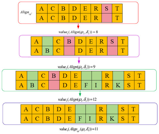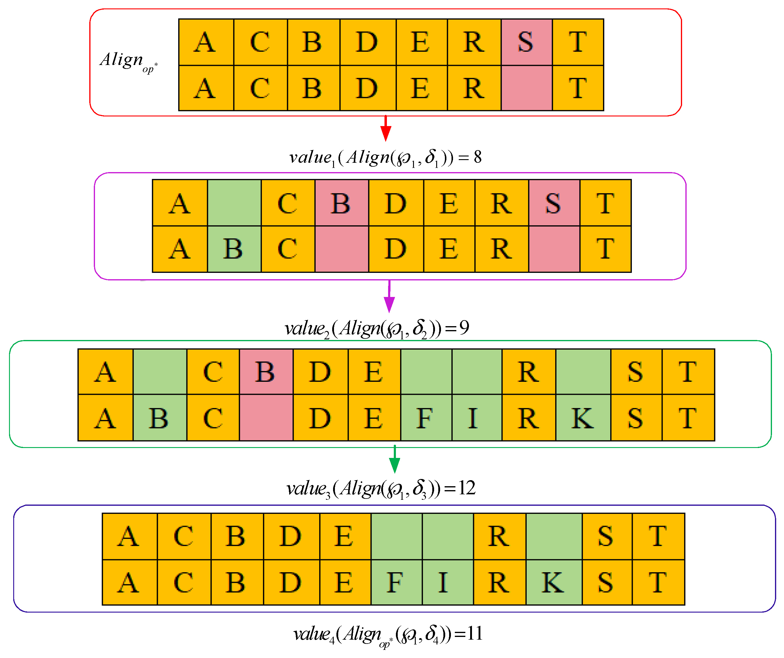The optimal alignment  $Alig{n}_{op}^{\ast }$ is the minimum cost alignment set associated with all traces, that is, $\cos t(Align({\wp }_o,{\delta }_{op}))<\cos t(Align({\wp }_o,{\delta }_j))$, $Alig{n}_{op}^{\ast }={\displaystyle \sum _{o=1}^{\left|O\right|}{\displaystyle \sum _{op=1}^{\left|OP\right|}Alig{n}_{op}({\wp }_o,{\delta }_{op})}}$, $\forall {\delta }_j\in M\backslash {\delta }_{op}$, $\forall {\delta }_{op}\in M\backslash {\delta }_j$. In other words, all alignments between the event log and the process model are necessary to be obtained before accurately judging the optimal alignment. As shown in Figure 1, the search workload for the optimal alignment between event log $L$ and process model $M$ is $value({\displaystyle \sum _{o=1}^{\left|O\right|}{\displaystyle \sum _{j=1}^{\left|J\right|}Align({\wp }_o,{\delta }_j)}})=value({\displaystyle \sum _{j=1}^{4}compare({\wp }_1,{\delta }_j)})=40$ ($value$ represents the number of comparisons in the optimal alignment evaluation). The optimal alignment between $L$ and $M$ is $Alig{n}_{op}=({\wp }_1,{\delta }_1)$.

Figure 1. Search workload for the optimal alignment. Note: event log is $L=(ACBDERST)$, and process model is $M=(ACBDERT,ABCDERT,ABCDEFIRKST,ACBDEFIRKST)$.

Definition 5

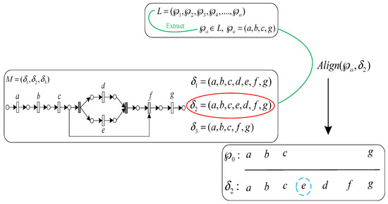
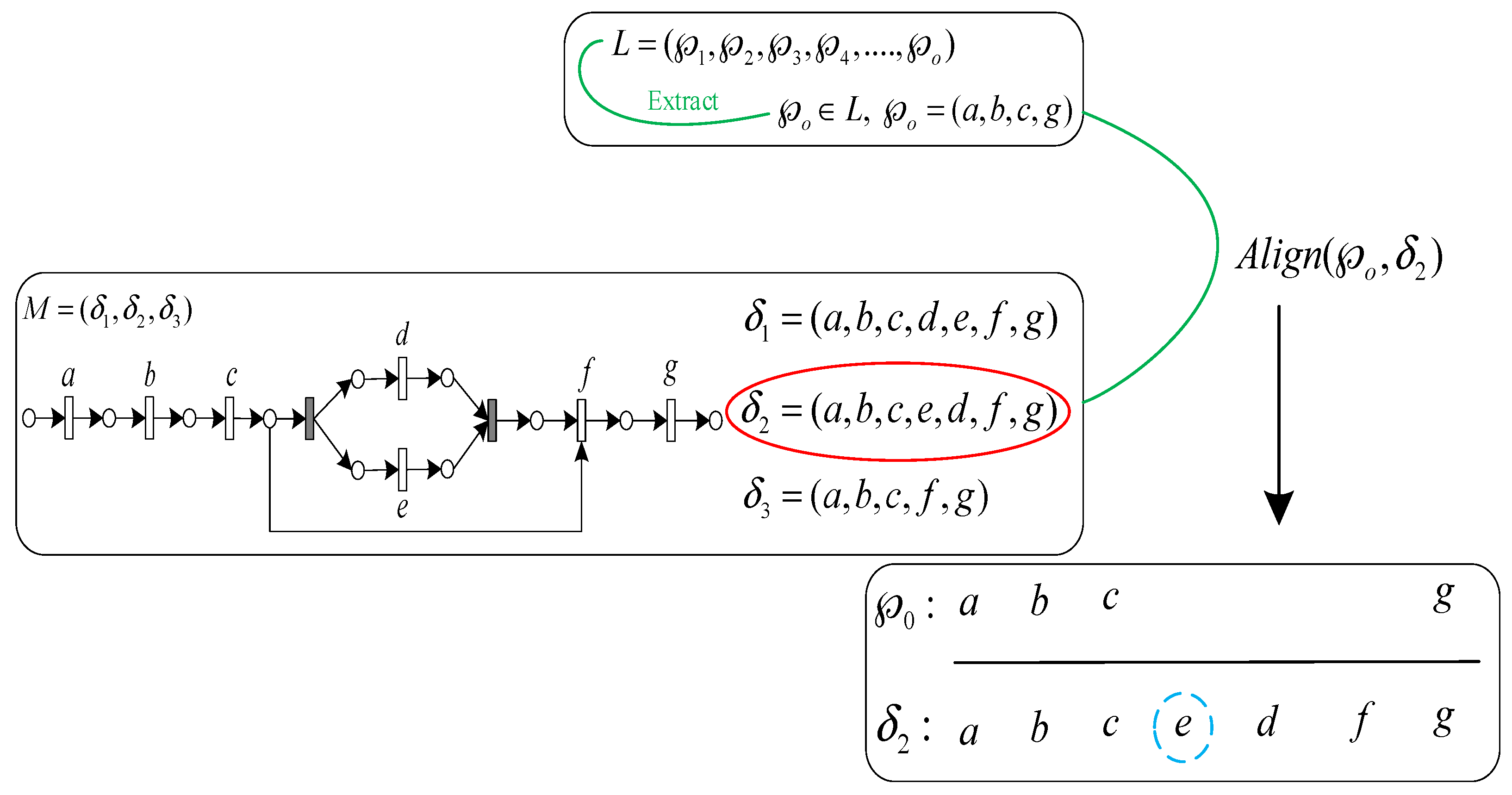
(Location of the initial deviation). The initial deviation is the first deviation in an alignment, and its location refers to the order of occurrence in an alignment. Figure 2 depicts the discovery process of the initial deviation. In Figure 2, a trace ${\wp }_0$ of $L$ and a sequence ${\delta }_2$ of $M$ are extracted, and the first difference $Skip(\lambda (t))=e$ produced by the alignment of ${\wp }_0$ and ${\delta }_2$ is marked with a dashed blue line. It is worth noting that the invisible transition $\tau$ in the model is ignored in order to better observe the deviation.

Figure 2. Discovery of initial deviation.

The initial deviation is detected in an alignment, and the location of the initial deviation is determined according to the unit order of alignment. The location of the initial deviation is denoted as $v(lo{c}_{id}(Align({\wp }_o,{\delta }_j)))$ (v is the evaluation function, that is, the location of moving unit in alignment is converted into numerical form; loc_id represents the occurrence location of the initial deviation in alignment). $Align({\wp }_1,{\delta }_1)$ and $Align({\wp }_1,{\delta }_2)$ in Table 2 are used as examples, and the asynchronous movement that produced the initial deviation $Esert(\mathcal{l}(e_3))=C$ is the third moving unit in $Align({\wp }_1,{\delta }_1)$. $v(lo{c}_{id}(Align({\wp }_1,{\delta }_1)))=3$ is obtained by the conversion of the evaluation function v, that is, the location of the initial deviation in $Align({\wp }_1,{\delta }_1)$ is 3. The asynchronous movement in $Align({\wp }_1,{\delta }_2)$ that produces the initial deviation $Skip(\lambda (t_2))=C$ is the second unit, which is transformed by the evaluation function v to obtain $v(lo{c}_{id}(Align({\wp }_1,{\delta }_2)))=2$, that is, the initial deviation in $Align({\wp }_1,{\delta }_2)$ occurs at 2. Therefore, the location of the initial deviation in $Align({\wp }_1,{\delta }_1)$ is greater than $Align({\wp }_1,{\delta }_2)$, denoted as $v(lo{c}_{id}(Align({\wp }_1,{\delta }_1)))>v(lo{c}_{id}(Align({\wp }_1,{\delta }_2)))$.

Table 2. Initial deviation locations of ξ₁ and ξ₂. Note: yellow is the initial deviation, $\xi$ is the identifier of $Align({\wp }_o,{\delta }_j)$.

ξ1	A	B	C	D	E	→	G
	A	B	→	→	E	F	G
ξ2	A	→	B	C	D	→	F
	A	C	B	→	→	E	F

Definition 6

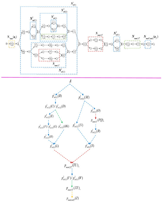
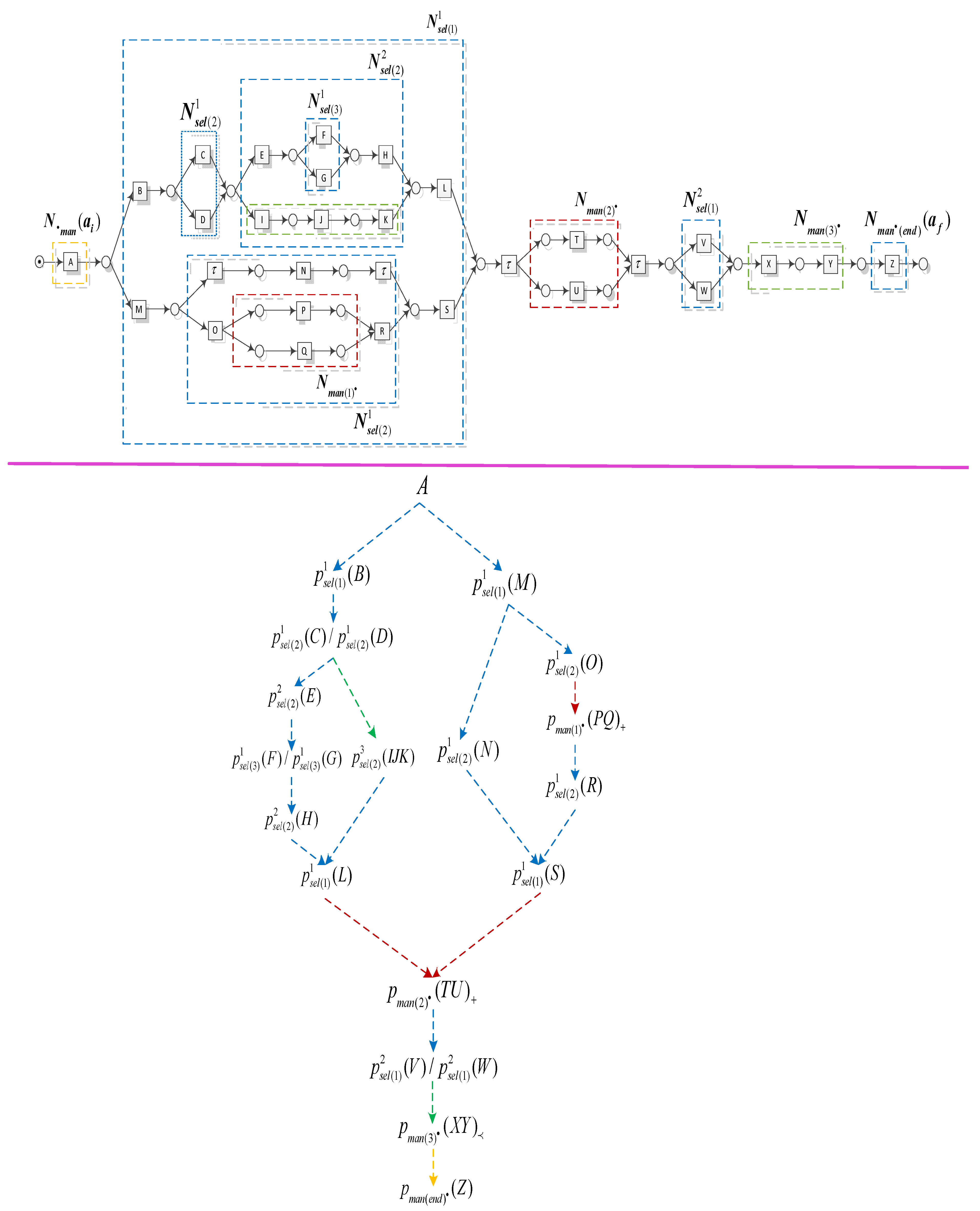
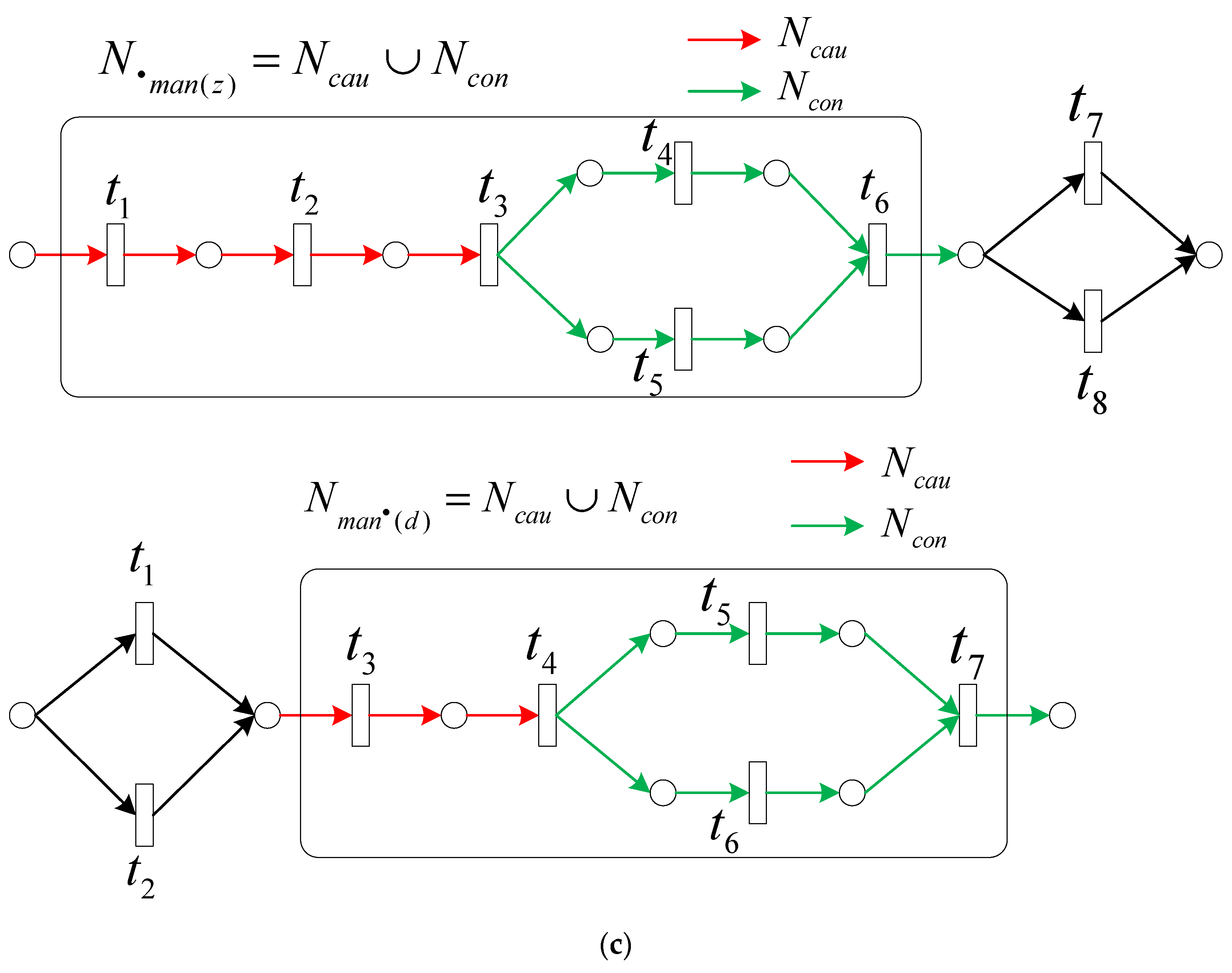
(Path partition of various substructures). Any path between the initial and the terminated nodes in a business process is called a complete path. Two types of sub-paths may be included in a complete path. Namely, a mandatory sub-path must occur, and a selective sub-path may occur, denoted as $p_{man}$, $p_{sel}$. The unique behavior on each complete path comes from $p_{sel}$, while the common behavior belongs to $p_{man}$. The substructure corresponding to $p_{man}$ is the mandatory substructure, that is, $\{N_{cau}\cup N_{conc}\}=N_{man}$. $N_{cau}$ and $N_{conc}$ satisfy causal and concurrent behavior, respectively. $N_{cau}$ and $N_{conc}$ both belong to mandatory substructures, that is, their activities occur on each complete path. $p_{sel}$ corresponds to the selective substructure, i.e., $N_{conf}=N_{sel}$ ($N_{cau}$ represents a substructure satisfying conflict behavior relationship). According to the above rules, the various substructures are divided and their corresponding sub-paths are given in Figure 3.

Figure 3. Division of paths in various substructures.

The level division of the selective substructure depends on the depth of selection. The selective substructure of the first level is regarded as the root of the tree structure. Then, the next level of the selective substructure is contained in the upper substructure, denoted as $N_{sel(leaf1)}\subset N_{sel(root)}$, $N_{sel(n)}\subset N_{sel(n-1)}$ ($N_{sel(leaf1)}$ represents the first leaf of the root structure, $n$ indicates the number of level division). According to the order of occurrence, the selective substructure of the same level can be denoted as $N_{sel(n)}^m$ ($m$ represents the number of occurrence order). The mandatory substructure can be divided into prepositive and postpositive substructures, which are denoted as $N_{{}^{·}man(z)}$ and $N_{ma{n}^{·}(d)}$. $N_{{}^{·}man\left(z\right)}$ and $N_{ma{n}^{·}(d)}$ are mandatory substructures that occur before and after the selective structure, respectively ($z$ and $d$ represent the occurrence orders of $N_{{}^{·}man(z)}$ and $N_{ma{n}^{·}(d)}$, respectively). It is worth noting that the types of all sub-paths in a substructure correspond to that of their substructures.

Definition 7

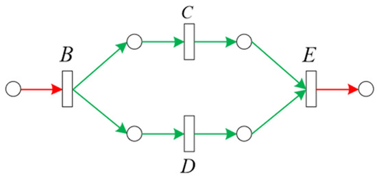
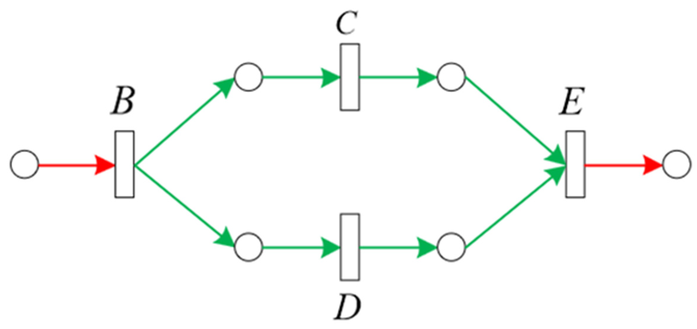
(Perceptible Region). The perceptible region is a set of special substructures in the process model, denoted as ${\phi }_{pM}^{\ast }\subseteq \{N_{sel(n)}^m\cup N_{{}^{·}man(z)}\cup N_{ma{n}^{·}(d)}\}$. A subalignment between a subsequence ${\delta }_j^{·}$ in ${\phi }_{pM}^{\ast }$ and any trace ${\wp }_o$ in the event log is denoted as$Alig{n}_{sub}({\wp }_o,{\delta }_j^{·})$. The subalignment set between ${\phi }_{pM}^{\ast }$ and ${\wp }_o$ is ${\displaystyle \sum _{j=1}^{\left|J\right|}Align({\wp }_o,{\delta }_j^{·})}=Alig{n}_{sub}^{\ast }({\wp }_o,{\delta }_j^{·})$. The smaller the initial deviation location, the larger the number of deviations in $Alig{n}_{sub}^{\ast }({\wp }_o,{\delta }_j^{·})$. A substructure $N_{conc}$ in ${\phi }_{pM}^{\ast }$ is described in Figure 4. ${\delta }_1^{·}=(BCDE)$ and ${\delta }_2^{·}=(BDCE)$ are included in $N_{conc}$. From Table 3, $Alig{n}_{sub}({\wp }_o,{\delta }_1^{·})$ is produced by ${\wp }_o=(ABCDFG)$ and ${\delta }_1^{·}=(BCDE)$. $Alig{n}_{sub}({\wp }_o,{\delta }_2^{·})$ is produced by ${\wp }_o=(ABCDFG)$ and ${\delta }_2^{·}=(BDCE)$. According to Definition 5, the location of the initial deviation in $Alig{n}_{sub}({\wp }_o,{\delta }_1^{·})$ and $Alig{n}_{sub}({\wp }_o,{\delta }_2^{·})$ is $v(lo{c}_{id}(Alig{n}_{sub}({\wp }_1^{·},{\delta }_1^{·})))=4>v(lo{c}_{id}(Alig{n}_{sub}({\wp }_1^{·},{\delta }_2^{·})))=2$. The cost of $Alig{n}_{sub}({\wp }_1^{·},{\delta }_1^{·})$ and $Alig{n}_{sub}({\wp }_2^{·},{\delta }_1^{·})$ is $\cos t(Alig{n}_{sub}({\wp }_1^{·},{\delta }_1^{·}))=1<\cos t(Alig{n}_{sub}({\wp }_1^{·},{\delta }_2^{·}))=3$.

Figure 4. Substructure N_conc of process model $M$.

Table 3. The subalignments $Alig{n}_{sub}({\wp }_o,{\delta }_1^{·})$ and $Alig{n}_{sub}({\wp }_o,{\delta }_2^{·})$. Note: the yellow is the initial deviation, and the gray has no practical meaning.

$Alig{n}_{sub}({\wp }_o,{\delta }_1^{·})$	B	C	D	→
	B	C	D	E
$Alig{n}_{sub}({\wp }_o,{\delta }_2^{·})$	B	C	D	→	→
	B	→	D	C	E

3. Recognition of the Perceptibility of Business Process

The search for optimal alignment aligns each trace with all firing sequences, and the alignment set is discovered by producing the minimum cost. In order to improve the search efficiency of the optimal alignment, the non-optimality of some alignments can be determined beforehand according to the specified condition in the perceptible region. The different substructures are divided based in the process model, and the perceptible region is determined by the behavioral characteristics of various substructures.

3.1. Establishment of Perceptibility Condition

The costs of all alignments corresponding to each trace are obtained, and the alignment with the minimum cost is evaluated (the number of deviations is equivalent to the cost of deviations if and only if the cost of each deviation is “1”). The optimal alignment between the event log and process model consists of all optimal trace alignments. Some non-optimal alignments can be predicted by the location of the initial deviation.

The location of the initial deviation in any alignment can be denoted as $v(lo{c}_{id}(Align({\wp }_o,{\delta }_j)))$ according to Definition 5. The location of the initial deviation in an alignment is not the largest when a trace is aligned with the process model. Then, this alignment must be non-optimal, denoted as the perceptibility condition $C_p:v(lo{c}_{id}(Align({\wp }_o,{\delta }_j))<v(lo{c}_{id}(Align({\wp }_o,{{\delta }^{\prime }}_j))\to \cos t(Align({\wp }_o,{\delta }_j))>\cos t(Align({\wp }_o,{{\delta }^{\prime }}_j))\to Align({\wp }_o,{\delta }_j)\notin Alig{n}_{op}^{\ast }$ ($\cos t$ is cost function). The comparisons of some non-optimal alignments are terminated at the location of the initial deviation when the perceptibility condition $C_p$ is satisfied. Therefore, the unnecessary alignments are saved. In order to take advantage of the given condition $C_p$, it is necessary to determine the perceptible region in the process model. For example, a trace in the event log ${\wp }_1=(ABDEK)$ is aligned with all firing sequences of the process model, shown in Figure 5. The location of the initial deviation in $Align({\wp }_1=(ABDEK),{\delta }_1=(ABGEFK))$ is $v(lo{c}_{id}(Align({\wp }_1,{\delta }_1)))=3$, and the number of deviations is also 3. The location of the initial deviation in $Align({\wp }_1=(ABDEK),{\delta }_2=(ABDHIJK))$ is $v(lo{c}_{id}(Align({\wp }_1,{\delta }_2)))=4$, and the number of deviations is also 4. $v(lo{c}_{id}(Align({\wp }_1,{\delta }_1)))<v(lo{c}_{id}(Align({\wp }_1,{\delta }_2)))$ and $\cos t(Align({\wp }_1,{\delta }_1))<\cos t(Align({\wp }_1,{\delta }_2))$, so $Align({\wp }_1,{\delta }_1)$ may be optimal. The above situation violates $C_p$.

Figure 5. Example of process model. Note: $N_{sel(1)}^1$ is represented by a green circle, and $N_{sel(1)}^2$ is marked by a red circle.

3.2. Determination of Perceptible Region

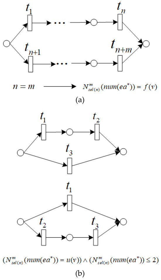
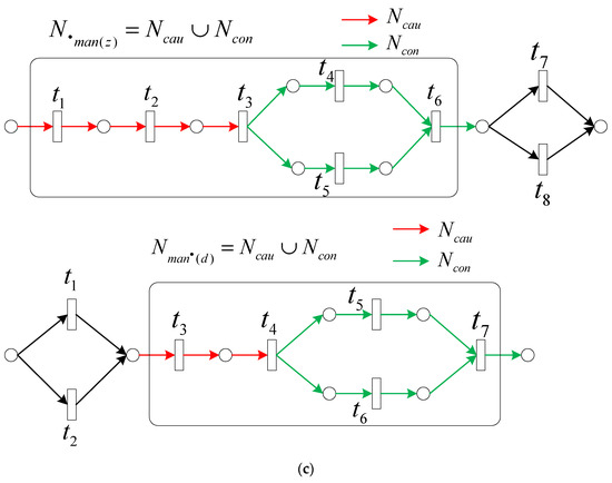
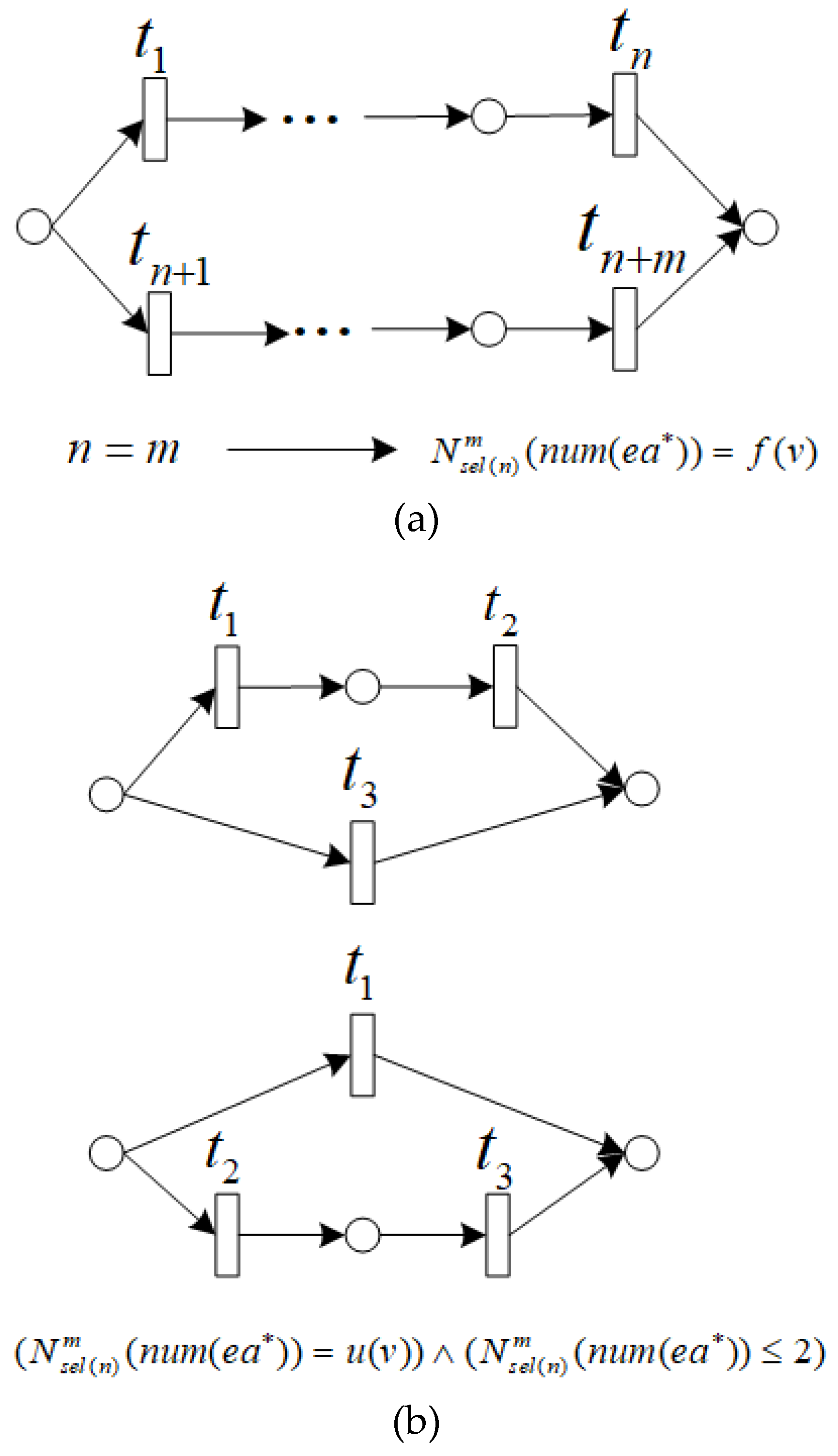
According to the example in Section 3.1, the perceptibility condition is not always satisfied. The perceptibility condition is valid if and only if the initial deviation occurs in the specific range. Therefore, it is necessary to determine the perceptible region based on the behavior characteristics of various substructures in the process model. There are four steps to determine the perceptible region in the process model: (i) according to Definition 6, various types of mandatory and selective substructures are divided in the process model; (ii) the initial node $a_i$ and the terminated node $a_f$ in the process model are determined and included in the perceptible region; (iii) according to Definition 6, the selective substructure with a fixed number of enable activities is denoted as $N_{sel(n)}^m(num(e{a}^{\ast }))=f(v)$. ($e{a}^{\ast }$ is a set of enabled activities,= that can occur; $f(v)$ is a fixed value). The given condition $C_p$ is satisfied by an alignment when the initial deviation occurs in $N_{{}^{·}man(z)}$, $N_{ma{n}^{·}(d)}$ and $N_{sel(n)}^m(num(e{a}^{\ast }))=f(v)$; (iv) it does not necessarily satisfy $C_p$, and the selective substructure with an uncertain number of enabled activities is denoted as $N_{sel(n)}^m(num(e{a}^{\ast }))=u(v)$($u(v)$ is a uncertain value). $C_p$ is satisfied when the number of enabling activities of $N_{sel(n)}^m(num(e{a}^{\ast }))=u(v)$ does not exceed 2 in any case, denoted as $N_{sel(n)}^m(num(e{a}^{\ast }))=u(v)\le 2$. Therefore, the whole perceptible region is denoted as ${\phi }_{pM}^{\ast }=\{a_i\cup N_{{}^{·}man(z)}\cup (N_{sel(n)}^m(num(e{a}^{\ast }))=f(v))\cup (N_{sel(n)}^m(num(e{a}^{\ast }))=u(v)\le 2)\cup N_{ma{n}^{·}(d)}\cup a_f\}$. It is denoted as $M\in {\phi }_{pM}^{\ast }$ when the process model contains only the substructures of the perceptible region. This is the reason why Figure 5 does not satisfy $C_p$, namely, $N_{sel(1)}^2(num(e{a}^{\ast }))=u(v)>2\to N_{sel(1)}^2\in {\phi }_{\neg pM}^{\ast }$ (${\phi }_{\neg pM}^{\ast }$ is the whole non-perceptible region, which is the set of all substructures that do not belong to the perceptible region ${\phi }_{pM}^{\ast }$). Figure 6a–c describes the three structures belonging to the perceptible region in the process model, respectively, i.e., $N_{sel(n)}^m(num(e{a}^{\ast }))=f(v)$, $N_{sel(n)}^m(num(e{a}^{\ast }))=u(v)\le 2$ and $N_{man}$($N_{{}^{·}man(z)}$, $N_{ma{n}^{·}(d)}$).

Figure 6. Various substructures belonging to the perceptible region in the process model. Selective substructure with the same number of enable activities (a), selective structure with the number of enable activities ≤ 2 (b), and mandatory substructure (c).

The determinate process of the perceptible region is described in Algorithm 1. Firstly, the initial and the terminated activities belong to the perceptible region (lines 1–3). Secondly, two mandatory substructures are located correctly, which belong to the perceptible region (lines 4–17). The selective substructure in which the number of the enabled activities is a fixed value in the process model is located correctly. Then, this selective substructure is assigned to the perceptible region (lines 22–24). The selective substructure is assigned to the perceptible region when the number of enabled activities is uncertain and the total number of enabled activities does not exceed 2 (lines 25–27). The selective substructure does not belong to the perceptible region when the number of enabled activities is uncertain and the total number of enabled activities exceeds 2 (lines 28–30). Finally, the output of Algorithm 1 is the perceptible range of the process model, denoted as ${\phi }_{pM}^{\ast }$.

Algorithm 1 Determine perceptible range

Input: $\begin{array}{l}\mathrm{process} \mathrm{model} M, a_i \mathrm{is} \mathrm{the} \mathrm{initial} \mathrm{activity}, a_f \mathrm{is} \mathrm{the} \mathrm{terminated} \mathrm{activity}, \mathrm{process} \mathrm{model} \\ \mathrm{substructure} N, \mathrm{pre}-\mathrm{function} pre\left(\right), \mathrm{post}-\mathrm{function} post(), \mathrm{the} \mathrm{numerical} \mathrm{function} \mathrm{num}\left(\right)\\ \mathrm{the} \mathrm{function} \mathrm{of} \mathrm{fixed} \mathrm{value} fv(), \mathrm{the} \mathrm{function} \mathrm{of} \mathrm{uncertain} uv(), \mathrm{the} \mathrm{set} \mathrm{of} \mathrm{enable} \mathrm{activities}\\ e{a}^{\ast }.\end{array}$

$\begin{array}{l}\mathrm{Output}: \mathrm{the} \mathrm{non}-\mathrm{perceptible} \mathrm{area} {\phi }_{pM}^{\ast }.\\ 1: \mathrm{If} a_i,a_f\in M and a_i=pre(a^{*}\backslash a_i) and a_f=post(a^{*}\backslash a_f) \mathrm{then}\\ 2:\hspace{1em} a_i,a_f\in {\phi }_{pM}^{\ast }\\ 3: \mathrm{end}\\ 4: z=1\\ 5: \mathrm{For} \mathrm{each} \mathrm{z}\in Z \mathrm{do} \\ 6: \mathrm{If} N_{{}^{·}man(z)}\in M \mathrm{and} N_{{}^{·}man(z)}=pre(N_{sel(n)}^m) \mathrm{then} \\ 7: N_{{}^{·}man(z)}\in {\phi }_{pM}^{\ast } \\ 8: \mathrm{end}\\ 9: z=z+1\\ 10: \mathrm{end} \\ 11: d=1\\ 12: \mathrm{For} \mathrm{each} d\in D \mathrm{do}\\ 13: \mathrm{If} N_{ma{n}^{·}(d)}\in M \mathrm{and} N_{ma{n}^{·}(d)}=post(N_{sel(n)}^m) \mathrm{then}\\ 14: N_{ma{n}^{·}(d)}\in {\phi }_{pM}^{\ast } \\ 15: \mathrm{end}\\ 16: d=d+1\\ 17: \mathrm{end}\\ 18: n=1\\ 19: \mathrm{For} n\in num(n) \mathrm{do}\\ 20: m=1\\ 21: \mathrm{For} m\in num(m) \mathrm{do}\\ 22: \mathrm{If} N_{sel(n)}^m\in M \mathrm{and} num(e{a}^{\ast })=f(v) \mathrm{then}\\ 23: N_{sel(n)}^m\in {\phi }_{pM}^{\ast }\\ 24: \mathrm{end}\\ 25: \mathrm{If} N_{sel(n)}^m\in M \mathrm{and} num(e{a}^{\ast })=u(v) \mathrm{then}\\ 26: \mathrm{If} num(e{a}^{\ast })\le 2 \mathrm{then} \\ 27: N_{sel(n)}^m\in {\phi }_{pM}^{\ast }\\ 28: \mathrm{else}\\ 29: N_{sel(n)}^m\notin {\phi }_{pM}^{\ast }\\ 30: \mathrm{end}\\ 31: \mathrm{end}\\ 32: m=m+1\\ 33: \mathrm{end}\\ 34: n=n+1 \\ 35: \mathrm{end}\\ 36: \mathrm{return} {\phi }_{pM}^{\ast }\end{array}$

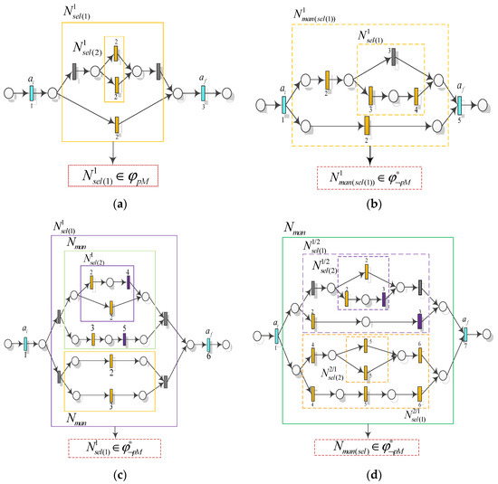
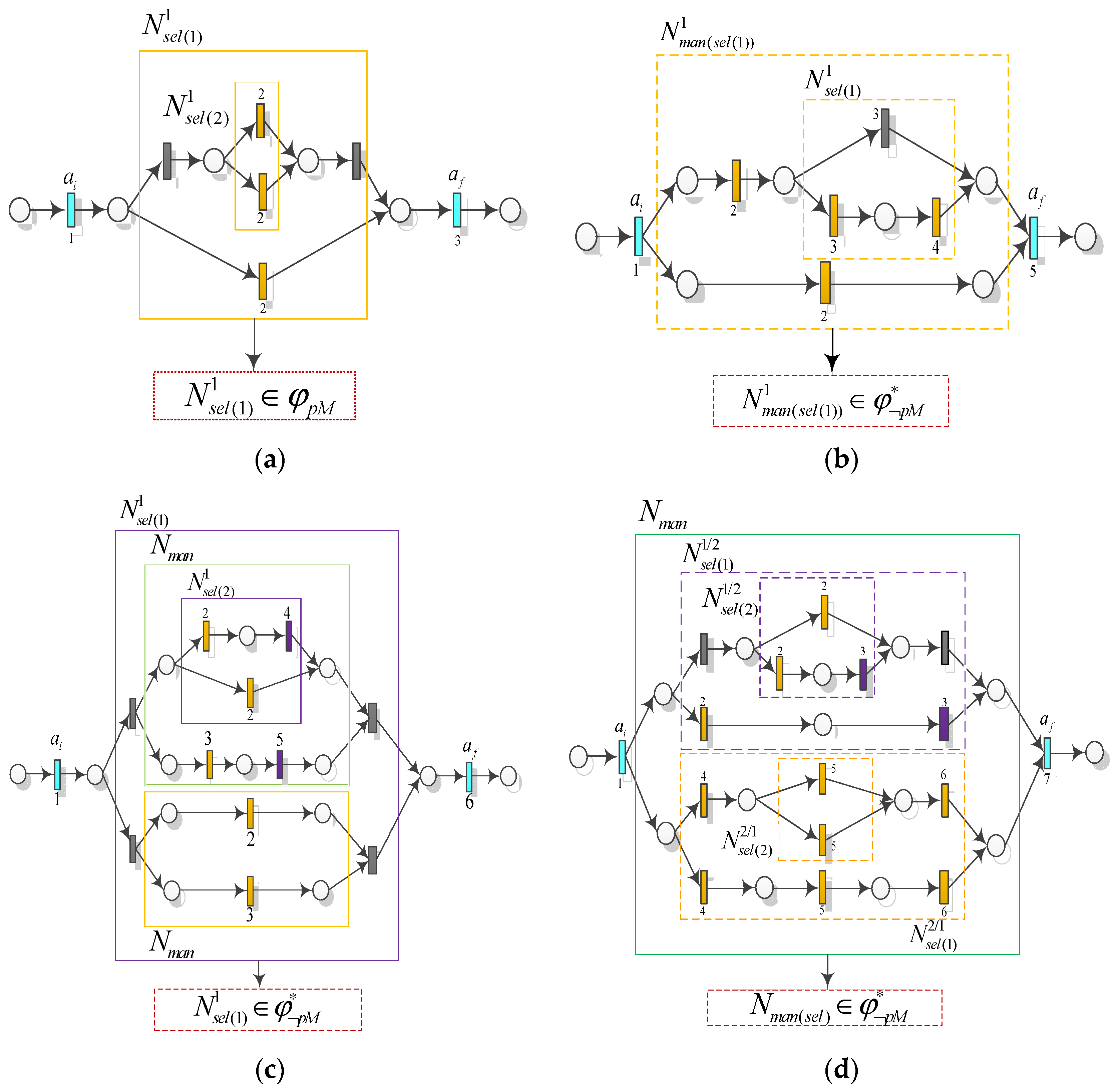
The substructure of a real-life business process can contain various nested types [41]. Four common nested substructures are described in Figure 7. The perceptible nested substructure needs to be analyzed according to the specific situation.

Figure 7. The perceptible range of nested substructures. Nested substructure $N_{sel(2)}^1\subset N_{sel(1)}^1$ (a); nested substructure $N_{sel(1)}^1\subset N_{man(sel(1))}^1$ (b); nested substructure $N_{man}\supset N_{sel(1)}^1$ (c); nested substructure $N_{sel(1)}^{(1/2)/(2/1)}\subset N_{man}$ (d).

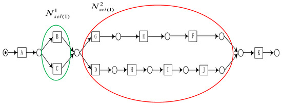
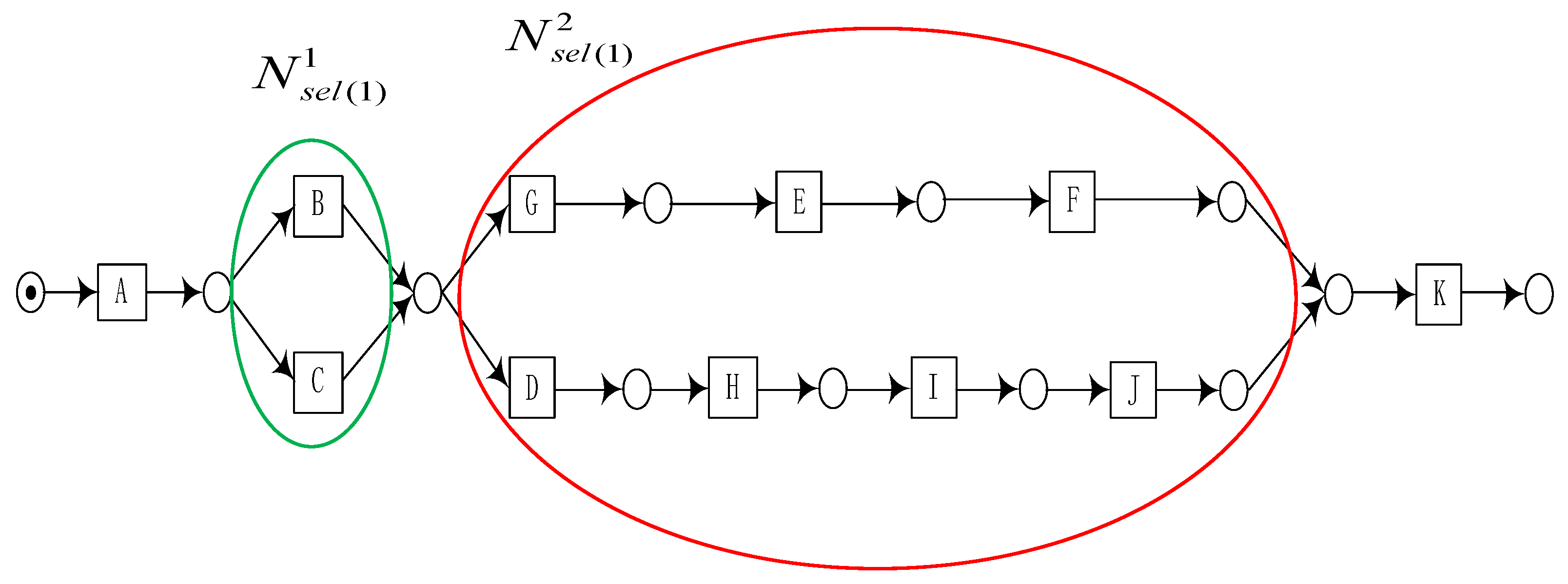
The selective substructure in $N_{\mathit{sel}\left(2\right)}^1$ in Figure 7a is contained in the selective substructure $N_{\mathit{sel}\left(1\right)}^1$, and the number of enabled activities of $N_{sel(1)}^1$ is 1. Thus, $N_{sel(1)}^1\in {\phi }_{pM}$. The selective substructure $N_{sel(1)}^1$ is contained in the mandatory substructure $N_{man}$, shown in Figure 7b. The mandatory substructure $N_{{}^{·}man}$ is regarded as a special selective substructure $N_{man(sel(1))}^1$. $N_{man(sel(1))}^1(num(e{a}^{\ast }))\ne f(v)$ and $\max (N_{man(sel(1))}^1(num(e{a}^{\ast })))=4>2$, so $N_{man(sel(1))}^1\in {\phi }_{\neg pM}^{\ast }$ ($\max$ is the maximum function). As shown in Figure 7c, two mandatory substructures $N_{man}$ are contained in the selective substructure $N_{sel(1)}^1$. The selective substructure $N_{sel(2)}^1$ is contained in one of the mandatory substructures $N_{man}$. $N_{sel(1)}^1(num(e{a}^{\ast }))\ne f(v)$ and $\max (N_{sel(1)}^1(num(e{a}^{\ast })))=4>2$, so $N_{sel(1)}^1\in {\phi }_{\neg pM}^{\ast }$. Two selective substructures $N_{sel(1)}^{1/2}$ and $N_{sel(1)}^{2/1}$ are contained in the mandatory substructure $N_{man}$, shown in Figure 7d, denoted as $N_{man(sel(1))}^{1/2}$ and $N_{man(sel(1))}^{2/1}$. $m=1/2$ and $m=2/1$, so the occurrence order of $N_{sel(1)}^{1/2}$ and $N_{sel(1)}^{2/1}$ is uncertain according to Definition 6. $N_{sel(2)}^{1/2}$ and $N_{sel(2)}^{2/1}$ are contained in $N_{man(sel(1))}^{1/2}$ and $N_{man(sel(1))}^{2/1}$, respectively. The structural property of $N_{man}$ is regarded as the selective substructure $N_{man(sel)}$. $N_{man(sel)}(num(e{a}^{\ast }))\ne f(v)$ and $\max (N_{man(sel)}(num(e{a}^{\ast })))=5>2$ in $N_{man(sel)}$, so $N_{man(sel)}\in {\phi }_{\neg pM}^{\ast }$. To sum up, the perceptible nested substructure needs to obey the following two rules: (i) the perceptibility condition of the selective substructure is directly considered when the outermost structure is the selective substructure; (ii) the mandatory substructure is judged to be a perceptible substructure if it does not contain a selective substructure. Otherwise, the mandatory substructure needs to be judged as the type of selective substructure.

The determination of perceptible nested substructure is described in Algorithm 2. The perceptible region is determined according to the normal rule of selective substructure when a mandatory substructure is contained in a selective substructure (lines 2–14). The mandatory substructure is regarded as a selective substructure if a selective substructure is contained in this mandatory substructure (lines 15–17).

Algorithm 2 Determine the perceptibility of nested substructures

Input: $\begin{array}{l}\mathrm{process} \mathrm{model} M, \mathrm{mandatory} \mathrm{concurrency} \mathrm{substructure} N_{man}, \mathrm{selective} \mathrm{substructure} N_{sel},\\ \mathrm{the} \mathrm{set} \mathrm{of} \mathrm{enable} \mathrm{activities} e{a}^{\ast }, \mathrm{function} \mathrm{of} \mathrm{fixed} \mathrm{value} fv(), \mathrm{function} \mathrm{of} \mathrm{maximum} \mathrm{value}\\ \max (), \mathrm{function} \mathrm{of} \mathrm{judge} \mathrm{substructure} N \mathrm{is} \mathrm{a} \mathrm{perceptive} \mathrm{region} j_N().\end{array}$

$\begin{array}{l}\mathrm{Output}: \mathrm{judge} \mathrm{result} yes \mathrm{or} no.\\ 1:\forall N_{man}\in M,\forall N_{sel}\in M\\ 2: \mathrm{If} N_{man}\subseteq N_{sel} \mathrm{and} N_{sel(man)}\in M \mathrm{then} \\ 3: \mathrm{If} e{a}^{\ast }\in N_{sel(man)} \mathrm{then}\\ 4: \mathrm{If} fv(e{a}^{\ast })=yes\\ 5: j_N(N_{sel(man)})=yes\\ 6: \mathrm{else}\\ 7: \mathrm{If} \max (e{a}^{\ast })\le 2 \mathrm{then} \\ 8: j_N(N_{sel(man)})=yes\\ 9: \mathrm{else}\\ 10: j_N(N_{sel(man)})=no\\ 11: \mathrm{end}\\ 12: \mathrm{end}\\ 13: \mathrm{end}\\ 14: \mathrm{end}\\ 15: \mathrm{If} N_{sel}\subseteq N_{man} \mathrm{and} N_{man(sel)}\in M \mathrm{then} \\ 16: N_{man(sel)}⊳N_{sel}\\ 17: j_N(N_{man(sel)})=j_N(N_{sel})\\ 18: \mathrm{end} \end{array}$

3.3. Reverse Search for Perceived Range

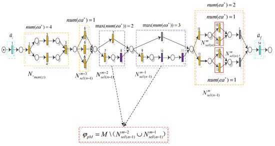
There are many types of substructures in process models, which are divided according to the occurrence possibility of each path in the substructure. Therefore, the type of each substructure between the initial and end nodes is determined for accurately detecting the perceptible and non-perceptible regions in the process model. The perceptible region in the process model is searched back-to-front according to Definition 6, which is called a reverse search. Figure 8 describes the process of a reverse search. Since $N_{sel(n)}^m\subset N_{sel(n-1)}^m$, $N_{sel(n)}^m$ and $N_{sel(n-1)}^m$ are regarded as a whole. $N_{sel(n-1)}^m(num(e{a}^{\ast }))=2$ indicates that the number of enabled activities in $N_{sel(n-1)}^m$ is a constant of 2, that is, $N_{sel(n-1)}^m\in {\phi }_{pM}^{\ast }$. $\max (N_{sel(n-1)}^{m-1}(num(e{a}^{\ast })))=3$ indicates that one branch of $N_{sel(n-1)}^{m-1}$ contains only a hidden transition, while the number of enabled activities on the other branch is 3, i.e., $N_{sel(n-1)}^{m-1}\in {\phi }_{\neg pM}^{\ast }$. $\max (N_{sel(n-1)}^{m-2}(num(e{a}^{\ast })))=2$ indicates that the maximum number of enable activities of $N_{sel(n-1)}^{m-2}$ is 2, that is, $N_{sel(n-1)}^{m-2}\in {\phi }_{pM}^{\ast }$. $N_{sel(n-1)}^{m-3}(num(e{a}^{\ast }))=1$ indicates that the number of enabled activities in $N_{sel(n-1)}^{m-3}$ is a constant of 1, that is, $N_{sel(n-1)}^{m-3}\in {\phi }_{pM}^{\ast }$. $N_{{}^{·}man(z)}(num(e{a}^{\ast }))=4$ is the number of enabled activities of $N_{{}^{·}man(z)}$, which is a constant, that is, $N_{{}^{·}man(z)}\in {\phi }_{pM}^{\ast }$. Thus, the perceptible range in Figure 8 is ${{\phi }_{pM}^{\ast }}^{\prime }=M\backslash (N_{sel(n-1)}^{m-2}\cup N_{sel(n-1)}^{m-1})$. The perceptibility condition of $C_p$ can be used to determine the optimal alignment when the initial deviation occurs in the perceptible region.

Figure 8. The reverse search for perceptible range. Note: numbers are marked at the locations of all activities in the process model, and the activities of the selective substructure that are in the same location can be recorded as the same number.

The reverse search for the perceptible region is described in Algorithm 3. Firstly, it is determined that various substructures belong to the process model (line 1). $N_{sel(n)}^m$ is not contained in $N_{ma{n}^{·}(d)}$; then, $M_{{\phi }_{pM}^{\ast }}\leftarrow N_{ma{n}^{·}(d)}$ (lines 3–6). Otherwise, $N_{ma{n}^{·}(d)}$ is regarded as $N_{sel(n)}^m$, and the algorithm jumps to line 10 (lines 7–9). The number of enabled activities of $N_{sel(n)}^m$ is determined to be a fixed value from the back forward, then $M_{{\phi }_{pM}^{\ast }}\leftarrow N_{sel(n)}^m$ (lines 13–17). The number of enabled activities of $N_{sel(n)}^m$ is not a fixed value and the maximum number of enabled activities does not exceed 2; then, $M_{{\phi }_{pM}^{\ast }}\leftarrow N_{sel(n)}^m$ (lines 18–21). The level $n$ is reduced by 1 if the next substructure satisfies $N_{sel(n-1)}^m\supset N_{sel(n)}^m$ (lines 22–24). The occurrence order $m$ is reduced by 1 if the substructure $N_{sel(n)}^{m-1}$ is the preceding substructure of $N_{sel(n)}^m$ (lines 25–27). $M_{{\phi }_{pM}^{\ast }}\leftarrow N_{ma{n}^{·}(z)}$ if $N_{sel(n)}^m$ is not contained in $N_{ma{n}^{·}(z)}$ (lines 29–32). Otherwise, $N_{{}^{·}man(z)}$ is regarded as $N_{sel(n)}^m$, and the algorithm returns to line 10 (lines 33–35). Finally, the output is the perceptible region of the process model $M_{{\phi }_{PM}^{\ast }}$ (line 37).

Algorithm 3 Non-perceivable areas are eliminated by reverse search

Input: $\begin{array}{l}\mathrm{process} \mathrm{model} M, \mathrm{mandatory} \mathrm{substructure} N_{man}, \mathrm{selective} \mathrm{substructure} N_{sel},\\ \mathrm{perceivable} \mathrm{range} \mathrm{of} \mathrm{process} \mathrm{model} M_{{\phi }_{PM}^{\ast }},\mathrm{initial} \mathrm{activity} a_i,\mathrm{final} \mathrm{activity} a_f,\\ \mathrm{perceptible} \mathrm{condition} C_p, \mathrm{fixed} \mathrm{value} fv, \mathrm{function} \mathrm{of} \mathrm{judge} \mathrm{substructure} N \mathrm{is} \\ \mathrm{a} \mathrm{perceivable} \mathrm{region} j().\end{array}$

$\begin{array}{l}\mathrm{Output}: \mathrm{perceivable} \mathrm{range} \mathrm{of} \mathrm{process} \mathrm{model} M_{{\phi }_{PM}^{\ast }}.\\ 1: \forall N_{man}\in M,\forall N_{sel}\in M\\ 2: d=\left|d\right|\\ 3: \mathrm{For} \mathrm{each} d\ge 1 \mathrm{do}\\ 4: \mathrm{If} N_{sel(n)}^m\not\subset N_{ma{n}^{·}(d)} \mathrm{then} \\ 5: j(N_{ma{n}^{·}(d)})=yes\\ 6: M_{{\phi }_{PM}^{\ast }}\leftarrow N_{ma{n}^{·}(d)}\wedge C_p(N_{ma{n}^{·}(d)})=true\\ 7: \mathrm{else}\\ 8: N_{ma{n}^{·}(d)}⊳N_{sel(n)}^m \mathrm{and} \mathrm{jump} \mathrm{to} 10 \mathrm{line} \\ 9: \mathrm{end}\\ 10: d=d-1 \\ 11: \mathrm{end}\\ 12: n=num(n)\wedge m=num(m)\\ 13: \mathrm{For} \mathrm{each} n\ge 1 \wedge m\ge 1 \mathrm{do}\\ 14: \mathrm{If} N_{sel(n)}^m\in M \wedge \mathrm{num}(e{a}^{\ast })=fv \wedge e{a}^{\ast }\in N_{sel(n)}^m \mathrm{then}\\ 15: j(N_{sel(n)}^m)=yes\\ 16: M_{{\phi }_{PM}^{\ast }}\leftarrow N_{sel(n)}^m\wedge C_p(N_{sel(n)}^m)=true\\ 17: \mathrm{end}\\ 18: \mathrm{If} N_{sel(n)}^m\in M \wedge \mathrm{num}(e{a}^{\ast })\ne fv \wedge 0\le num(e{a}^{\ast })\le 2 \wedge e{a}^{\ast }\in N_{sel(n)}^m \mathrm{then}\\ 19: j(N_{sel(n)}^m)=yes\\ 20: M_{{\phi }_{PM}^{\ast }}\leftarrow N_{sel(n)}^m\wedge C_p(N_{sel(n)}^m)=true\\ 21: \mathrm{end}\\ 22: \mathrm{If} \exists N_{sel(n-1)}^m\supset N_{sel(n)}^m \mathrm{then} \\ 23: n=n-1\\ 24: \mathrm{end}\\ 25: \mathrm{If} \exists N_{sel(n)}^{m-1}=pre(N_{sel(n)}^m) \mathrm{then}\\ 26: m=m-1\\ 27: \mathrm{end} \\ 28: \mathrm{end}\\ 29: \mathrm{For} \mathrm{each} z\ge 1 \mathrm{do}\\ 30: \mathrm{If} N_{sel(n)}^m\not\subset N_{ma{n}^{·}(z)} \mathrm{then} \\ 31: j(N_{ma{n}^{·}(z)})=yes\\ 32: M_{{\phi }_{PM}^{\ast }}\leftarrow N_{ma{n}^{·}(z)}\wedge C_p(N_{ma{n}^{·}(z)})=true\\ 33: \mathrm{else}\\ 34: N_{ma{n}^{·}(z)}⊳N_{sel(n)}^m \mathrm{and} \mathrm{return} \mathrm{to} 10 \mathrm{line} \\ 35: \mathrm{end}\\ 36: \mathrm{end} \\ 37: \mathrm{Return} M_{{\phi }_{pM}^{\ast }} \end{array}$

4. Perceptible Search for Optimal Alignment

Each trace is aligned with all firing sequences by the optimal alignment, and the alignment that satisfies the least deviation cost is selected. The brute force search will produce a huge amount of computation for the complex business process. It is proposed that the non-optimality of alignment is perceived based on the location of the initial deviation, thereby reducing some unnecessary comparisons.

4.1. Perceptible Search Algorithm

The optimal alignments of the event log can be regarded as a sum of the optimal alignment of each trace since the event log contains different traces. The search for optimal alignment is denoted as $Search(Alig{n}_{op}^{\ast }(L,M))=Search({\displaystyle \sum _{o=1}^{\left|O\right|}{\displaystyle \sum _{op=1}^{\left|OP\right|}Align({\wp }_o,{\delta }_{op})})}$. The default location of the initial deviation of each trace is recorded as 0, denoted as $v(lo{c}_{id}(Align({\wp }_o,M)))=0$. According to the perceptibility condition $C_p$, an alignment cannot be judged to be non-optimal when $v(lo{c}_{id}(Align({\wp }_o,{\delta }_j)))\ge v(lo{c}_{id}(Align({\wp }_o,M)))$. Therefore, the final cost of $Align({\wp }_o,{\delta }_j)$ needs to be obtained and evaluated together with the other alignments of ${\wp }_o$, namely, $(Alig{n}^{\ast }({\wp }_o,M)\leftarrow Align({\wp }_o,{\delta }_j))\wedge h_{op}(Alig{n}^{\ast }({\wp }_o,M))$ ($h_{op}$ is the evaluated function of the minimum cost). In this case, $v(lo{c}_{id}(Align({\wp }_o,{\delta }_j)))$ is assigned to the record value $v(lo{c}_{id}(Align({\wp }_o,M)))$, and acts as the perceptible standard for the next alignment $Align({\wp }_o,{\delta }_{j+1})$. This alignment must not be the optimal alignment of ${\wp }_o$ when $v(lo{c}_{id}(Align({\wp }_o,{\delta }_j)))<v(lo{c}_{id}(Align({\wp }_o,M)))$. Therefore, a complete comparison of $Align({\wp }_o,{\delta }_j)$ is not needed, and $v(lo{c}_{id}(Align({\wp }_o,M)))$ remains unchanged. It is worth noting that the perceptibility condition is feasible when the initial deviation occurs in the perceptible region. The overall process of the perceptible algorithm is described in Figure S1.

The above search for optimal alignment can be denoted as $Alig{n}_{op}^{\ast }(L,M)\leftarrow PS({\displaystyle \sum _{o=1}^{\left|O\right|}{\displaystyle \sum _{j=1}^{\left|J\right|}Align({\wp }_o,{\delta }_j)})}$. It can directly jump to the next trace ${\wp }_{o+1}$ when ${\wp }_o$ is consistent with ${\delta }_j$, and this alignment is regarded as the optimal alignment of ${\wp }_o$. The concrete procedures and the proof of perceptible search ($PS$) are described in the Supplementary Materials.

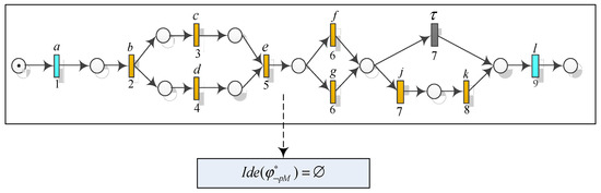
The process model $M$ with the perceptible location is described in Figure 9, and the non-perceptible region is not contained in $M$, namely, $Ide({\phi }_{\neg pM}^{\ast })=\varnothing$. All the firing sequences of $M$ are recorded in Table 4.

Figure 9. The process model $M$ without non-perceivable region.

Table 4. A set of firing sequences of $M$.

Serial No.	Occurrence Sequence
δ1	(a,b,c,d,e,f,j,k,l)
δ2	(a,b,c,d,e,g,l)
δ3	(a,b,c,d,e,f,l)
δ4	(a,b,c,d,e,g,j,k,l)
δ5	(a,b,d,c,e,f,l)
δ6	(a,b,d,c,e,g,l)
δ7	(a,b,d,c,e,f,j,k,l)
δ8	(a,b,d,c,e,g,j,k,l)

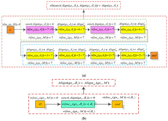
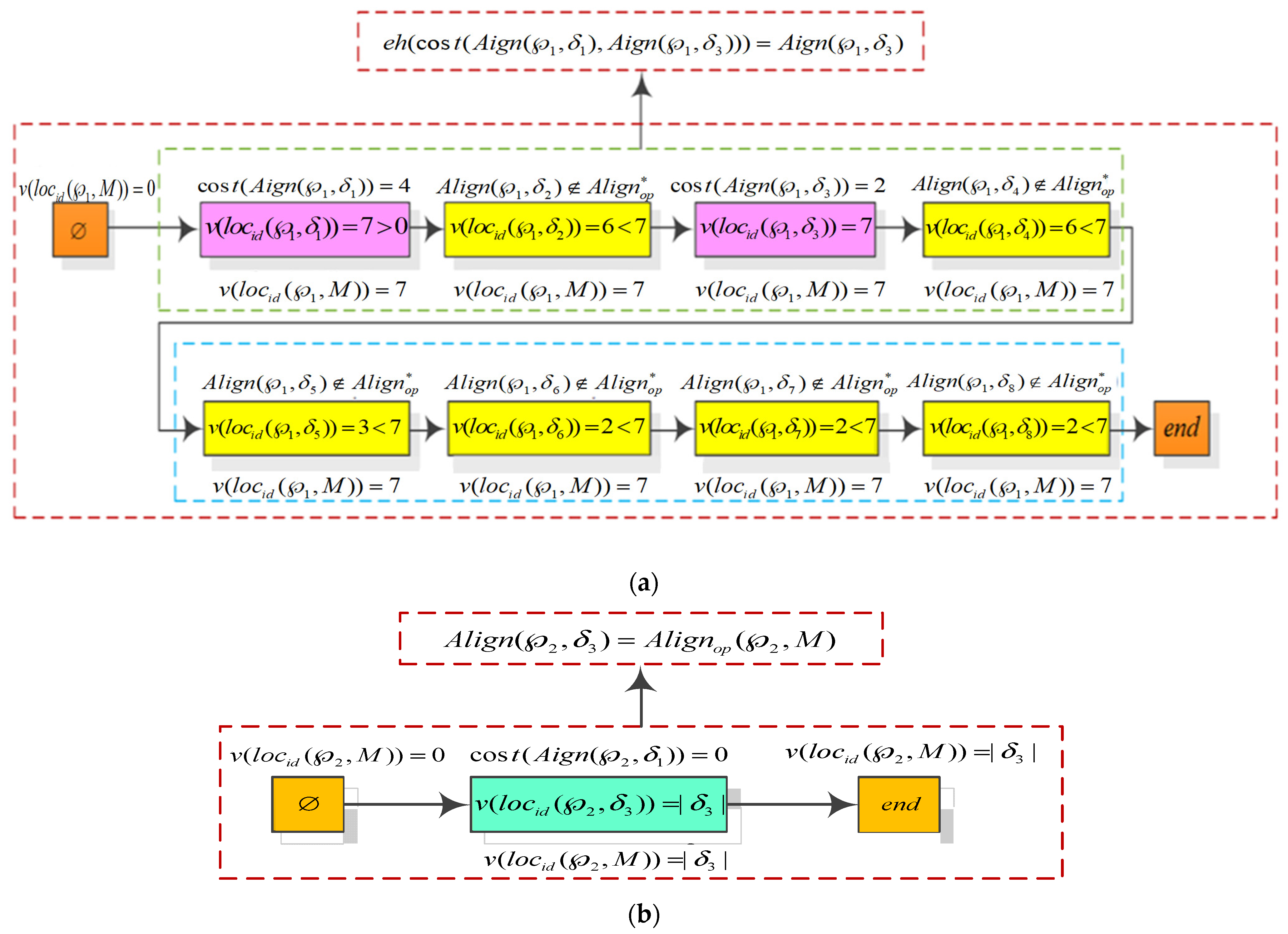
The event log is set to L = {(a,b,c,d,e,f,h,i,l),(a,b,c,d,e,f,j,k,l,)}. $L$ is aligned with $M$, and the search process of the optimal alignment is depicted in Figure 10. Figure 10a,b is the search process for traces ${\wp }_1$ and ${\wp }_2$, respectively. From Figure 10a, the location of the initial deviation in the first and the third alignment is greater than or equal to the previously recorded value. These two alignments need to be evaluated, that is, $v(lo{c}_{id}(Alig{n}^{\ast \prime }({\wp }_1,{\delta }_{1,3})))\ge v(lo{c}_{id}(Alig{n}^{\ast \prime }({\wp }_1,M)))\to Wcompare(Alig{n}^{\ast \prime }({\wp }_1,{\delta }_{1,3}))$. The location of the initial deviation in other alignments is smaller than the previously recorded value. These alignments are directly judged to be non-optimal, denoted as $v(lo{c}_{id}(Alig{n}^{\ast ″}({\wp }_1,{\delta }^{\ast }\backslash {\delta }_{1,3})))<v(lo{c}_{id}(Alig{n}^{\ast ″}({\wp }_1,M)))\to Pcompare(Alig{n}^{\ast ″}({\wp }_1,{\delta }^{\ast }\backslash {\delta }_{1,3}))\to Alig{n}^{\ast ″}({\wp }_1,{\delta }^{\ast }\backslash {\delta }_{1,3})\notin Alig{n}_{op}^{\ast }$ ($Pcompare$ is the function of partial comparison). For example, $v(lo{c}_{id}(Align({\wp }_1,{\delta }_2)))=6<7$ and $Align({\wp }_1,{\delta }_2)=Pcompare(Align({\wp }_1,{\delta }_2))$. The comparison of $Align({\wp }_1,{\delta }_2)$ is terminated when the initial deviation occurs. From Figure 10b, the first alignment has no deviation, so it is directly judged as the optimal alignment of ${\wp }_2$.

Figure 10. Search for the set of optimal alignments. Note: $v(lo{c}_{id}({\wp }_1,{\delta }_1))$ is simplification for $v(lo{c}_{id}(Align({\wp }_1,{\delta }_1)))$. Note: the pink block represents the alignments of complete comparison, the yellow block shows the alignments of partial comparison and the green block represents the fitting alignment. The search process of optimal alignment between ${\wp }_1$ and $M$ (a), and the search process of optimal alignment between ${\wp }_2$ and $M$ (b).

Algorithm 4 describes the perceptible search for optimal alignment. The set of optimal alignments is initialized to the $\varnothing$ (line 1). The recorded location of the initial deviation is set to 0 (line 4). The alignment needs to be completely compared and the location of the initial deviation is assigned to the recorded value if the location of the initial deviation is greater than or equal to the previously recorded value in perceptible region (lines 7–9). The recorded value is maintained and the comparison of alignment is terminated when the location of the initial deviation is smaller than the previously recorded value (lines 10–13). The recorded value is maintained and the alignment is completely compared if the initial deviation of alignment occurs in a non-perceptible region (lines 15–17). The alignment is regarded as the optimal alignment of a trace if no deviation is found between the trace and firing sequence (lines 18–21). All alignments that need complete comparison are assigned to the alignment set $Alig{n}^{\ast }$ (line 22). The optimal alignment set $Alig{n}_{op}^{\ast }$ is evaluated by $h_{op}$ (line 25). The optimal alignment set is output between the event log and process model as a result (line 28).

Algorithm 4 Search the optinal alignment based on the location of initial deviation

Input: $\begin{array}{l}\mathrm{event} \log L, \mathrm{process} \mathrm{model} M, \mathrm{trace} {\wp }_o, \mathrm{firing} \mathrm{sequence} {\delta }_j, \mathrm{the} \mathrm{value} \mathrm{of} \mathrm{initial} \mathrm{deviation} \mathrm{location} v(lo{c}_{id}({\wp }_o,M)),\\ \mathrm{the} \mathrm{perceptible} \mathrm{range} {\phi }_{pM}^{\ast }, \mathrm{the} \mathrm{non}-\mathrm{perceptible} \mathrm{range} {\phi }_{\neg pM}^{\ast }, \mathrm{the} \mathrm{evalution} \mathrm{function} \mathrm{of} \mathrm{the} \mathrm{optimal} \mathrm{alignment} h_{op}, \mathrm{the} \\ \mathrm{whole} \mathrm{compared} \mathrm{function} \mathrm{of} \mathrm{alignment} Wcompare, \mathrm{the} \mathrm{partial} \mathrm{compare} \mathrm{of} \mathrm{alignment} Pcompare, \mathrm{the} \mathrm{set} \mathrm{of} \mathrm{the} \mathrm{alignments}\\ \mathrm{is} Alig{n}_{op}^{\ast }. \end{array}$

$\begin{array}{l}\mathrm{Output}: \mathrm{the} \mathrm{set} \mathrm{of} \mathrm{the} \mathrm{alignments} \mathrm{is} Alig{n}_{op}^{\ast }.\\ 1:Alig{n}_{op}^{\ast }=\varnothing \\ 2: o=1 \\ 3: \mathrm{For} \mathrm{each} o\in O \mathrm{do}\\ 4: v(lo{c}_{id}({\wp }_o,M))=0\\ 5: j=1\\ 6: \mathrm{For} \mathrm{each} j\in J \mathrm{do} \\ 7: \mathrm{If} \cos t(Align({\wp }_o,{\delta }_j))>0 \wedge lo{c}_{id}(Align({\wp }_o,{\delta }_j))\subseteq N_{man/sel} \wedge N_{man/sel}\in {\phi }_{pM}^{\ast } \mathrm{then}\\ 8: \mathrm{If} v(lo{c}_{id}(Align({\wp }_o,{\delta }_j)))\ge v(lo{c}_{id}(Align({\wp }_o,M)))=0 \mathrm{then} \\ 9: Wcompare(Align({\wp }_o,{\delta }_j))\wedge v(lo{c}_{id}(Align({\wp }_o,M)))\leftarrow v(lo{c}_{id}(Align({\wp }_o,{\delta }_j)))\\ 10: \mathrm{else}\\ 11: |Pcompare(Align({\wp }_o,{\delta }_j)\left)\right|=v(lo{c}_{id}(Align({\wp }_o,{\delta }_j)))\\ 12: Pcompare(Align({\wp }_o,{\delta }_j))\wedge v(lo{c}_{id}(Align({\wp }_o,M)))\leftarrow v(lo{c}_{id}(Align({\wp }_o,M)))\wedge jump to 24 line\\ 13: \mathrm{end}\\ 14: \mathrm{end}\\ 15: \mathrm{If} \cos t(Align({\wp }_o,{\delta }_j))>0 \wedge lo{c}_{id}(Align({\wp }_o,{\delta }_j))\subseteq N_{man/sel} \wedge N_{man/sel}\in {\phi }_{\neg pM}^{\ast } \mathrm{then} \\ 16: Wcompare(Align({\wp }_o,{\delta }_j))\wedge v(lo{c}_{id}(Align({\wp }_o,M)))\leftarrow v(lo{c}_{id}(Align({\wp }_o,M)))\\ 17: \mathrm{end}\\ 18: \mathrm{If} \cos t(Align({\wp }_o,{\delta }_j))=0 \mathrm{then} \\ 19: Alig{n}_{op}^{\ast }\leftarrow Align({\wp }_o,{\delta }_j) \\ 20: jump to line 26\\ 21: \mathrm{end}\\ 22: Alig{n}^{\ast }\leftarrow Wcompare(Align({\wp }_o,{\delta }_j))\\ 23: j=j+1\\ 24: \mathrm{end}\\ 25: Alig{n}_{op}^{\ast }\leftarrow h_{op}(Alig{n}^{\ast })\\ 26: o=o+1\\ 27: \mathrm{end}\\ 28: \mathrm{return} Alig{n}_{op}^{\ast } \end{array}$

4.2. Example of Industrial Application

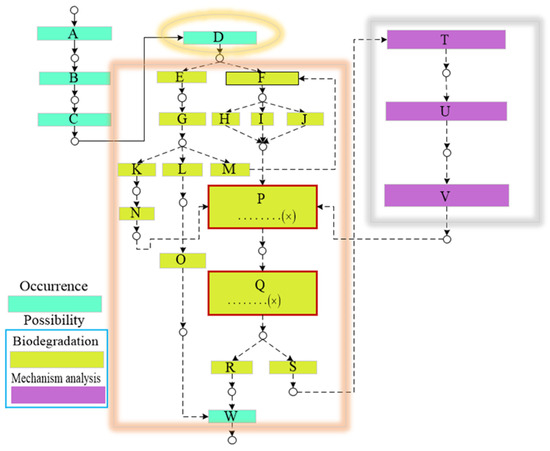
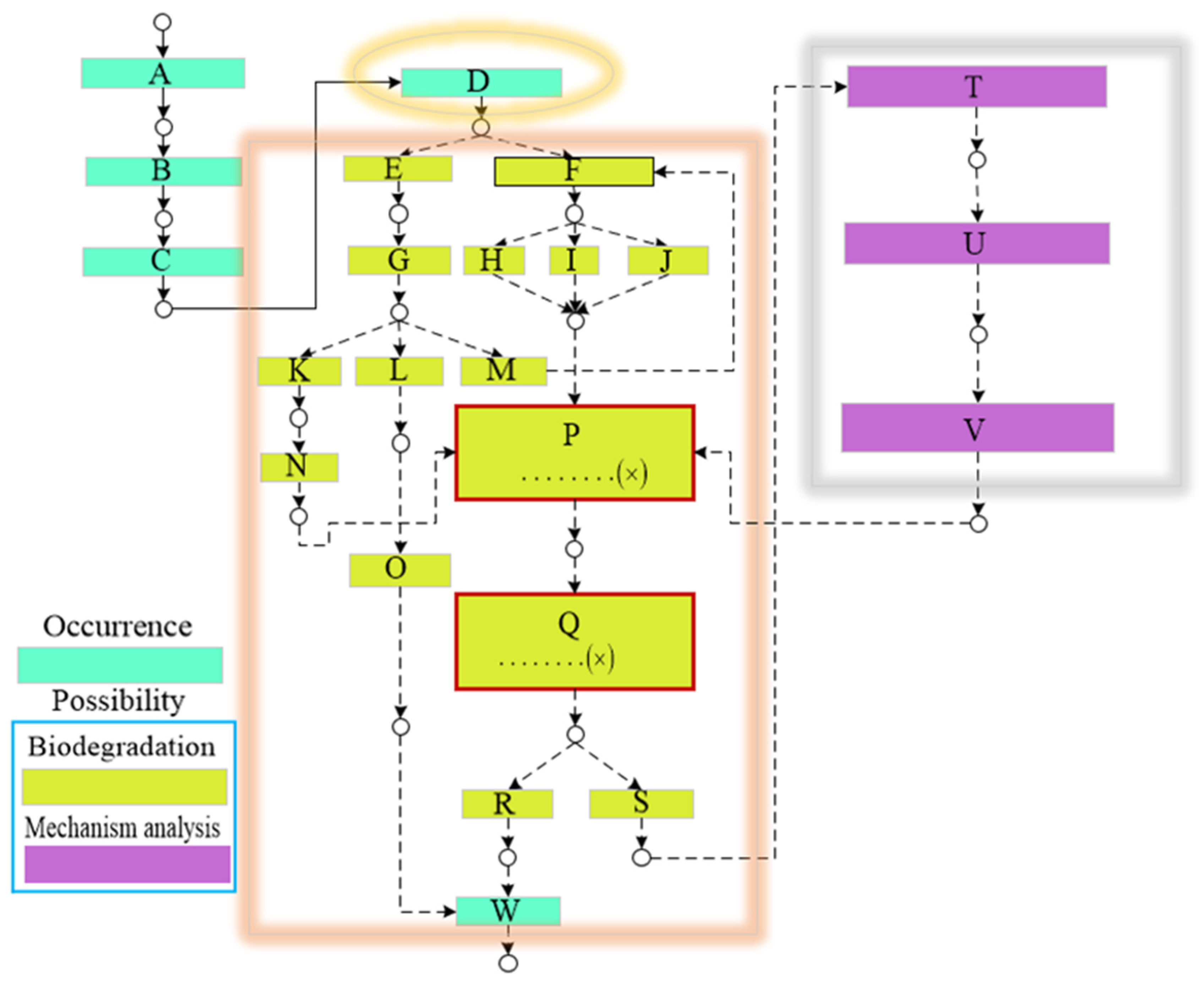
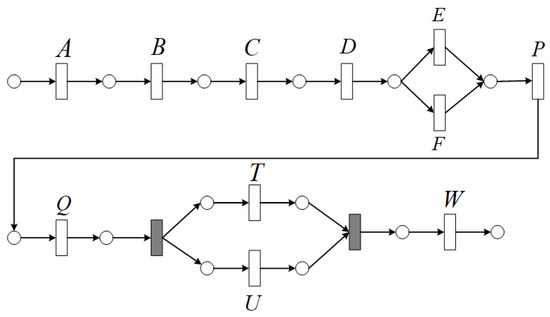
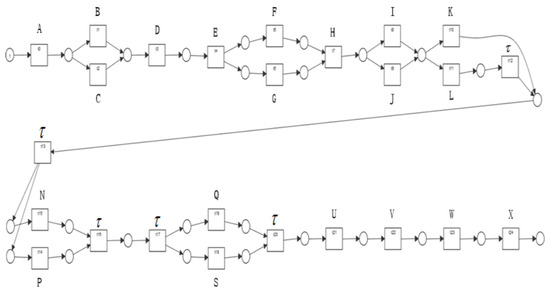
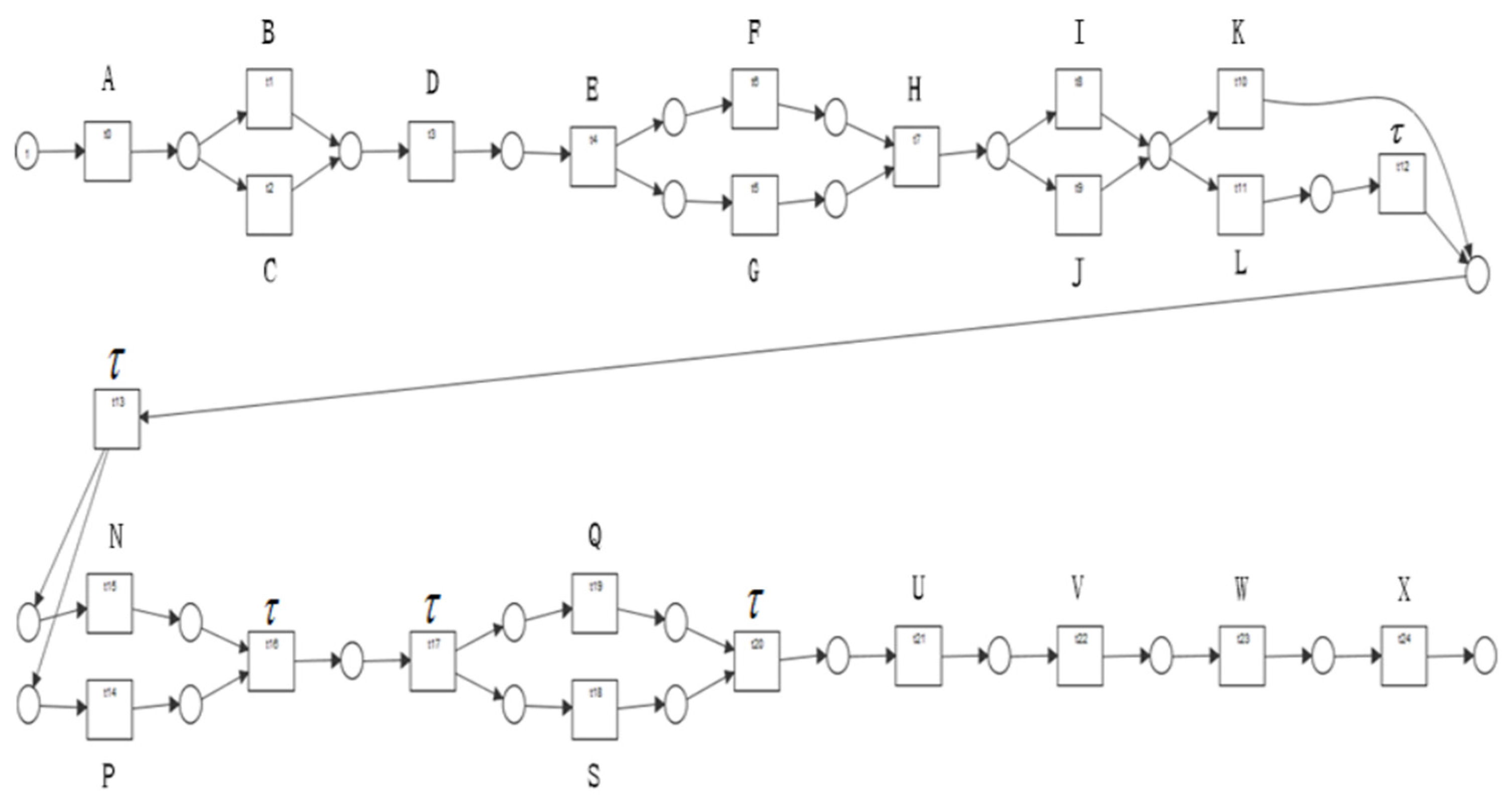
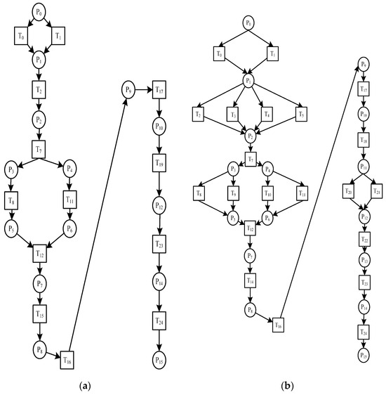
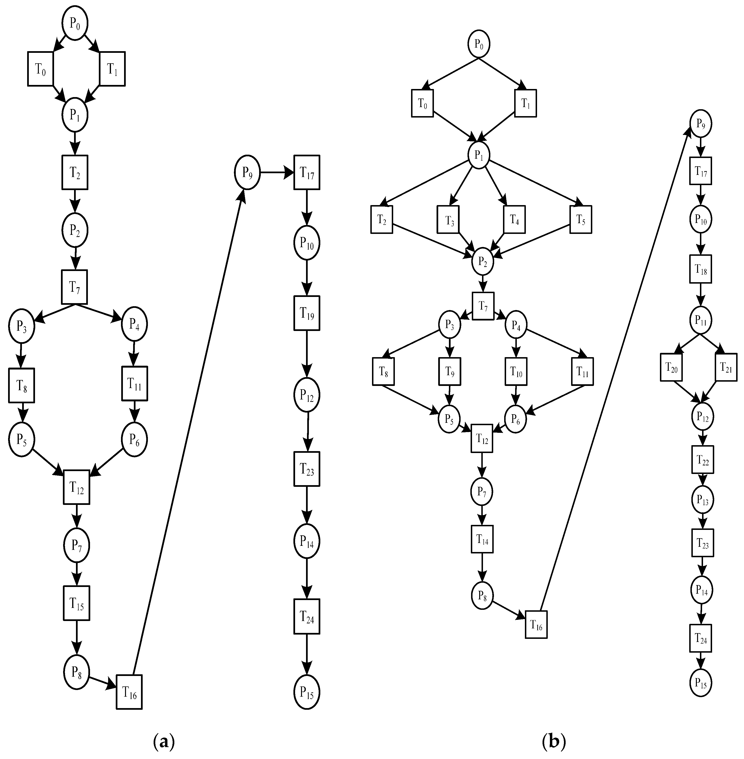
The behavior recorded in the initial process is often different from that described in the current information system due to the larger flow and complicated properties of coal slime water. The degradation performance of anionic polyacrylamide (HPAM) may be affected by different operational conditions. Therefore, the biological coal-washing process should be regarded as a business process that executes a specific goal. The deviation elements are detected in the actual biological coal-washing process, providing accurate technical support for the subsequent optimization. Figure 11 and Figure 12 describe the current process and initial model in the biological coal-washing using Petri net language, respectively. Table 5 lists annotations of the letter labels in Figure 11 and Figure 12.

Figure 11. Current business process of biological coal-washing process. Note: labels for the actual steps in the transition are replaced by letters.

Figure 12. Initial model of biological coal-washing process.

Table 5. Professional notes for letter labels.

Letter	Professional Note	Remark
A	Treatment of coal slime water
B	Pre-sedimentation
C	Enter the reaction pool
D	Add HPAM
E	Flocculation
F	Biodegradation
G	Monitoring concentration
H	Fungus
I	bacteria
J	Bio-enzyme
K	$<10\mathrm{mg}/\mathrm{L}$	This concentration range meets environmental emission standards.
L	$10–100\mathrm{mg}/\mathrm{L}$	This concentration range has no significant effect on coal flotation.
M	$>100\mathrm{mg}/\mathrm{L}$	The opposite of the above two cases ($<10\mathrm{mg}/\mathrm{L}$ and $10–100\mathrm{mg}/\mathrm{L}$).
N	Emission
O	Reuse
P	Real environment survey	The real-life environment contains many possibilities. This section has many selective behaviors.
Q	Optimization of reaction conditions based on machine learning	This section contains a number of selective operations based on the actual situation.
R	Yes
S	No
T	Computer molecular simulation
U	Research on the mechanism of enzymatic transformation
V	Enzymatic engineering design
W	Terminate

As shown in Figure 11, let trace ${\wp }_o=(ABCDEGKNPQSTUVPQRW)$ be recorded in $L$, and then, ${\wp }_o$ compares $M$ in Figure 12. The two firing sequences ${\delta }_j=(ABCDEPQUTW)$ and ${\delta }_{j^{\prime }}=(ABCDFPQTUW)$ are extracted for constructing two alignment $Align({\wp }_o,{\delta }_j)$ and $Align({\wp }_o,{\delta }_{j^{\prime }})$, respectively. According to the judgment of the perceptible region in Section 3.2, $M\in {\phi }_{pM}^{\ast }$ is known. $Align({\wp }_o,{\delta }_{j^{\prime }})$ can be determined to be non-optimal when the first deviation $Esert(\mathcal{l}(e_5))=E$ occurs due to $v(lo{c}_{id}(Align({\wp }_o,{\delta }_j)))=6>v(lo{c}_{id}(Align({\wp }_o,{\delta }_{j^{\prime }})))=5$. According to Theorem S1 in the Supplementary Materials, there exists ${\delta }_{j^{″}}=(ABCDEPQTUW)$ and it makes $Align({\wp }_o,{\delta }_{j^{″}})$ superior to $Align({\wp }_o,{\delta }_j)$ and $Align({\wp }_o,{\delta }_{j^{\prime }})$. Therefore, the efficiency of deviation detection in actual operation is effectively improved.

5. Evaluation

An experiment was performed on a 64-bit Win10 computer with Inter(R) Core(TM) i5-2.11 GHZ with 8 GB of memory space and python3.7. The $A^{\ast }$ algorithm needed to make the complete comparison of all alignments between the event log and process model, which was denoted as $A^{\ast }-Align$. $OI{A}^{\ast }-Align$ directly jumped to the alignment of the next trace if and only if an alignment that fit perfectly was found by it. The deviation perception proposed in this paper was denoted as $IDP-Align$, and its scalability and effectiveness were verified by the performance comparison of the above three methods.

5.1. The Operation Interface of OPS-Align Plug-In

$A^{\ast }-Align$ and $OI{A}^{\ast }-Align$ could be realized through the source code in the prom framework, but $IDP-Align$ could not. To ensure the fairness of the experimental results, we wrote a OPS-Align plug-in in Python to evaluate the search workload of the optimal alignment.

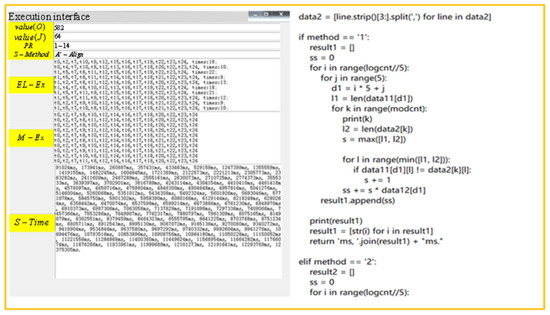
Figure 13 describes the OPS-Align plug-in interface. Input and output information were located in the left of the interface, and parts of the program code were located in the right. As shown in Figure 13, $value(O)$ was the total number of trace cases, $value(J)$ was the total number of firing sequences, $PR$ was the perceptible range, $S-Method$ was the current method, $EL-Ex$ was the event log used in the experiment, $M-Ex$ was the process model used in the experiment and $S-Time$ was the search time.

Figure 13. OPS-Align plug-in interface.

5.2. Scalability

In order to verify the improvement in various business processes, $A^{\ast }-Align$ and $IDP-Align$ could be evaluated on data sets with different network structures.

5.2.1. Data Sets of Artificial and Real-Life Business Process

Four artificial and two real-life data sets were used in the experiment. Each data set was constructed by ten different event logs and a corresponding initial model. Based on the initial model, these event logs were generated by redundancy activity, loss activity and dislocation between activities or cyclic substructure.

• Artificial data set.

Four artificial data sets were generated from two different artificial business processes. These two business processes were considered initial models $M_{a1}$ and $M_{a2}$, respectively. The non-perceptible range was not set in $M_{a1}$ and $M_{a2}$. Each artificial data set contained the selective substructure or the cyclic substructure.

• Real-life data set.

As shown in Figure 14, the auto-claim process mined by the prom framework was regarded as the initial model $M_r$ in the two real-life data sets. The activities of M, O, R and T were removed so that the non-perceptible region was not contained in $M_r$. The selective substructure and the cyclic substructure were contained in each real-life data set, so these data sets had a universal network structure.

Figure 14. Real-life business process mined by prom framework.

5.2.2. Experimental Results on Different Network Structures

• Artificial data sets with selective substructures.

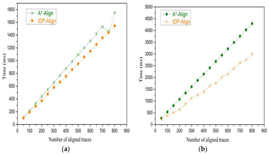
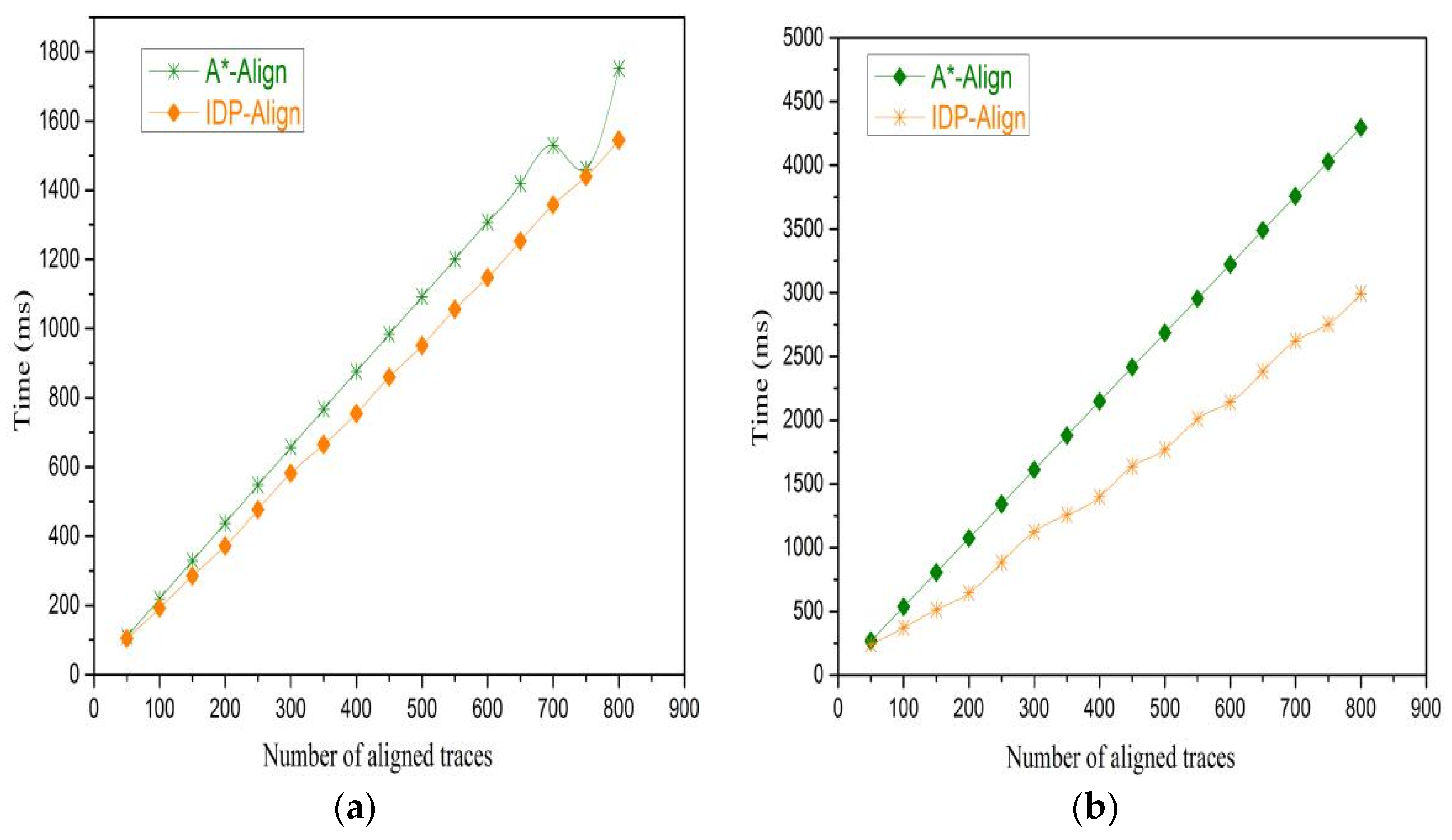
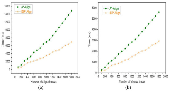
Figure 15 describes the performance of A^* − Align and IDP − Align in two data sets containing a selective substructure. The X and Y axes represented the number of aligned traces and the search time of the optimal alignment, respectively. Each trace was required compared with all firing sequences, so the number of aligned traces was referred to the total number of traces involved in the alignment process, denoted as $|Trac{e}_{align}|={\displaystyle \sum _{o=1}^{\left|O\right|}{\wp }_o}\times n\times num(J)$ ($n$ represents the number of repetition of ${\wp }_o$, and $num(J)$ is the total number of firing sequences). Each event log had 200 aligned traces, and ten data sets were analyzed, as shown in Figure 15a,b. Each data set was constructed of ten event logs and a corresponding initial model, that is, $D_{a1}^{\ast }(L_{a(1,\dots ,10)},M_{a1})$ and $D_{a2}^{\ast }({L^{″}}_{a(1,\dots ,10)},M_{a1})$. The average search time of ten data sets was taken to ensure the authenticity of the experimental result. The business processes in Figure 15a,b contained 11 and 23 activities, respectively. The length intervals of traces in two data sets were 6 to 8 and 14 to 20, respectively. The lengths of firing sequences in two data sets were 7 and 16, respectively. The search time using IDP − Align was reduced by 207 ms (in Figure 15a), while it was reduced by 1302 ms (in Figure 15b) compared to A^* − Align. From Figure 15, we found that the size of the data set was larger, and more activities could be automatically eliminated in perception. Thus, the difference in search time was greater.

Figure 15. The running results on the data sets with selective substructure. Run result of data set with 11 activities (a), and run result of data set with 23 activities (b).

• Artificial data sets with different cyclic substructures.

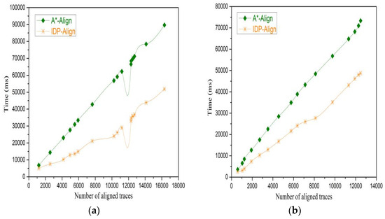
Each event log had 300 aligned traces, and ten data sets were analyzed, as shown in Figure 16a,b. Each data set was constructed of ten event logs and a corresponding initial model, that is, $D_{a3}^{\ast }({L^{″}}_{a(1,\dots ,10)},M_{a2})$ and $D_{a4}^{\ast }({L^{‴}}_{a(1,\dots ,10)},M_{a2})$. The average search time of ten data sets was taken to ensure the authenticity of the experimental result. Figure 16a,b contained 10 and 11 activities, respectively. The maximum length of the trace and firing sequence could not be determined due to the cyclic substructure in each data set. The cyclic substructures in Figure 16a,b were the self-loop and the loop of three activities, respectively. The search time using IDP − Align was reduced by 2700 ms (in Figure 16a), while it was reduced by 7908 ms (in Figure 16b) compared to A^* − Align. The size of alignment comparison was enlarged by the cyclic substructure, so more elements were automatically eliminated in perception (in Figure 16b). Thus, the improvement degree of search time depended on the size of the data set compared to the A^* − Align.

Figure 16. The running results of data sets with cyclic substructures. Run result of data set with 10 activities (a), and run result of data set with 11 activities (b).

• Real-life data sets with universal network structures.

The real-life data sets containing both selective substructures and cyclic substructures were evaluated. The cyclic substructures contained in Figure 17a,b were the self-loop and normal loop, respectively. Each event log had 1020 and 780 aligned traces, and ten data sets were analyzed as shown in Figure 17a,b, respectively. Each data set was constructed of ten event logs and a corresponding initial model $M_r$, that is, $D_{r1}^{\ast }(L_{r(1,\dots ,10)},M_r)$ and $D_{r2}^{\ast }({L^{\prime }}_{r(1,\dots ,10)},M_r)$. The average search time of ten data sets was taken to ensure the authenticity of the experimental result. The search time using IDP − Align was reduced by 37,752 ms (in Figure 17a), while it was reduced by 24,600 ms (in Figure 17b) compared to A^* − Align. This was due to the size of the data set and cyclic substructure.

Figure 17. Running results on generic data sets. Run result of data set with 1020 aligned traces (a), and run result of data set with 780 aligned traces (b).

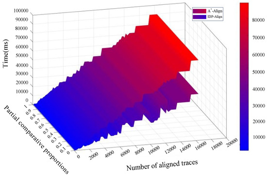
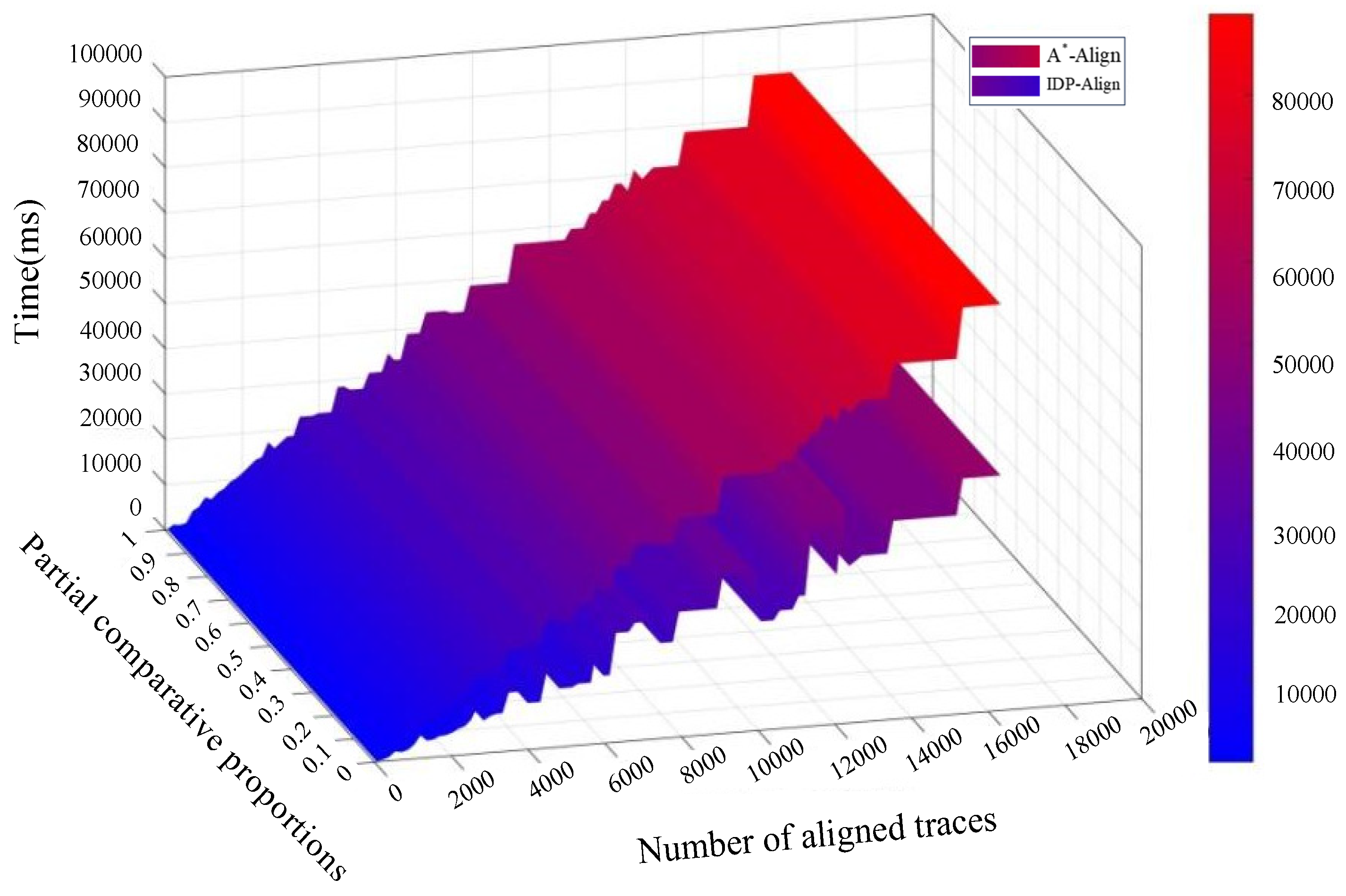
To sum up, the search time was significantly shortened by IDP − Align applied to various networks for the large-sized data sets. Figure 18 shows the experimental results of eight different data sets. Their parameters were search time, alignment proportion of partial comparisons and the number of aligned traces. The alignment proportion of partial comparisons was the ratio of automatically eliminated non-optimal alignments. In the same data set, the alignment proportion of partial comparisons was larger and the reduction of search time was more obvious than A^* − Align. As shown in Figure 18, the search time for data sets with various network structures could be effectively reduced using IDP − Align compared with A^* − Align.

Figure 18. Merging results of different data sets.

5.2.3. Experimental Results on Biological Coal-Washing Data Set

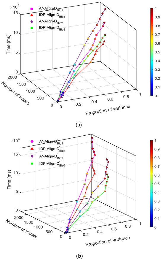
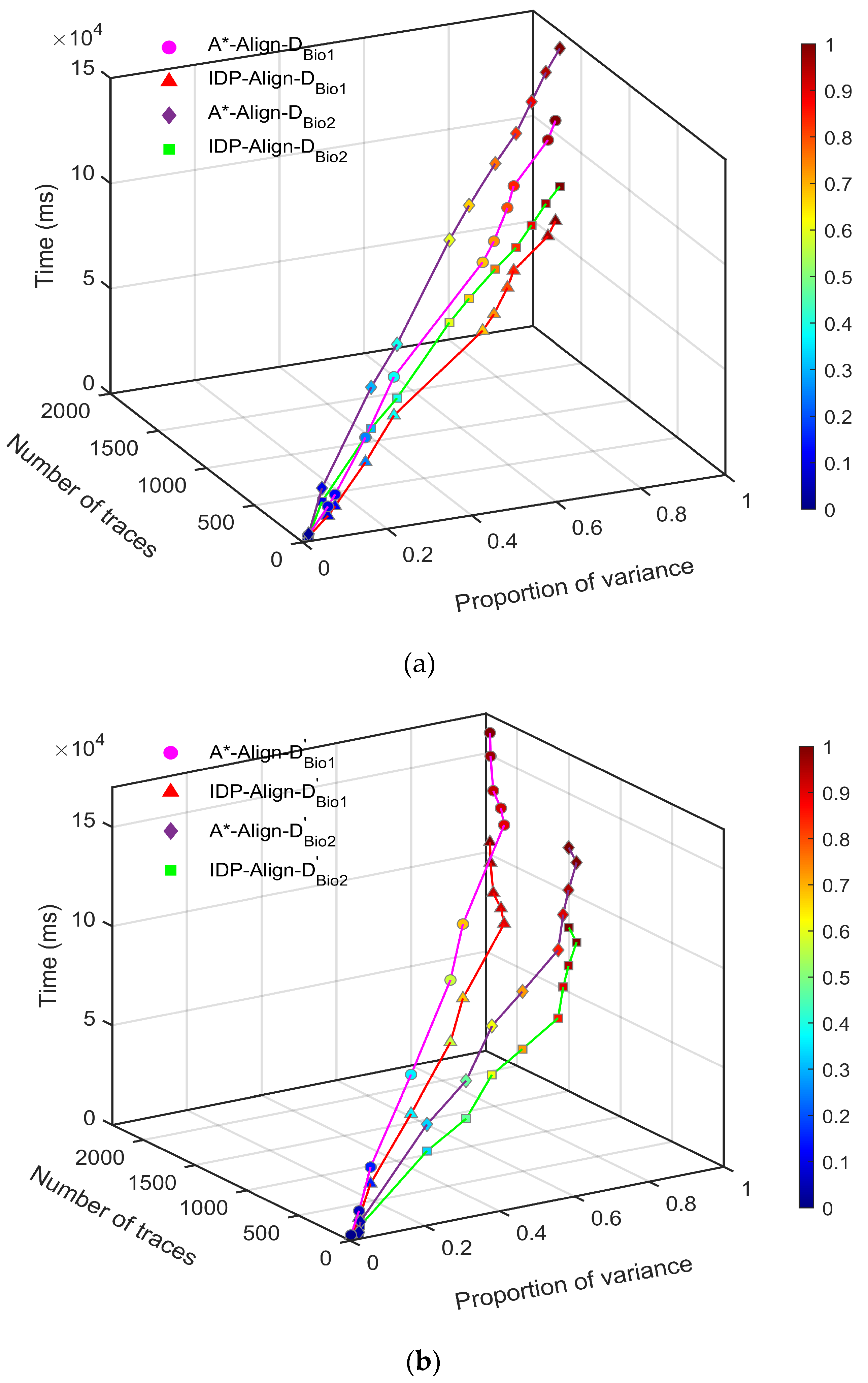
The biological coal-washing process was simulated as event logs, that is, $L_{Bio}$ without loop structure and ${L_{Bio}}^{\prime }$ with loop structure, respectively. The initial model is constructed by a simple process, $M_{Bio}$($M_{Bio}\in {\phi }_{pM}^{\ast }$) and ${M_{Bio}}^{\prime }$(${M_{Bio}}^{\prime }\in {\phi }_{pM}^{\ast }$), consisting of basic steps, respectively. The points of each line represent the search time and the proportion of time difference in data sets of different sizes (seen in Figure 19). As can be seen from Figure 19, the proportion of search time and time difference increases with the increase of data set size. As can also be seen from Figure 19, the search time and the proportion of time difference increases with the increase of data set size.

Figure 19. Evaluations of biological coal-washing data set. The results of $D_{Bio1}$ and $D_{Bio2}$ (a), and the results of ${D_{Bio1}}^{\prime }$ and ${D_{Bio2}}^{\prime }$ (b). Note: time indicates the search time for optimal alignment; the number of traces indicates the number of traces in the event log; proportion of variance represents the proportion of the current time difference in the total time difference.

From Figure 19a, $D_{Bio1}$ is composed of $L_{Bio}$ and $M_{Bio}$, while $D_{Bio2}$ is composed of ${L_{Bio}}^{\prime }$ and $M_{Bio}$. $A^{\ast }-Align$ and $IDP-Align$ are executed on these two data sets. The substructures in $D_{Bio1}$ were causal, concurrent and selective, that is, $N_{cau}$, $N_{conc}$ and $N_{sel(n)}^m$. However, $D_{Bio2}$ has more cyclic substructures than $D_{Bio1}$. As shown in Figure 19a, the search time of $IDP-Align$ in $D_{Bio1}$ and $D_{Bio2}$ was reduced by 47,648 ms and 65,768 ms compared with that of $A^{\ast }-Align$, respectively. From Figure 19b, ${D_{Bio1}}^{\prime }$ is composed of $L_{Bio}$ and ${M_{Bio}}^{\prime }$, while ${D_{Bio2}}^{\prime }$ is composed of ${L_{Bio}}^{\prime }$ and ${M_{Bio}}^{\prime }$. $A^{\ast }-Align$ and $IDP-Align$ are executed on these two data sets. As shown in Figure 19b, the search time of $IDP-Align$ in ${D_{Bio1}}^{\prime }$ and ${D_{Bio2}}^{\prime }$ was reduced by 55,226 ms and 40,232 ms compared with that of $A^{\ast }-Align$, respectively. The substructures in ${D_{Bio1}}^{\prime }$ were causal, concurrent and selective, that is, $N_{cau}$, $N_{conc}$ and $N_{sel(n)}^m$. However, ${D_{Bio2}}^{\prime }$ has more cyclic substructures than ${D_{Bio1}}^{\prime }$.

5.3. Effectiveness

$A^{\ast }-Align$, $OI{A}^{\ast }-Align$ and $LDP-Align$ were performed on two BPIC2020 data sets so as to verify the improvement of search efficiency on the basis of guaranteeing optimality. At the same time, the experiment took into account the different noises.

5.3.1. BPIC2020 Data Sets

The data sets used came from BPIC2020. Table 6 lists the specific information of the two event logs in BPIC2020. Their cases and event types represent the number of different traces and event elements, respectively. Domestic Declarations in BPIC2020 were used as the event log of the experiment. Figure 20a,b shows two process models $M_{B1}$ and $M_{B2}$ with inconsistent behavior from Domestic Declarations, respectively. The non-perceivable region was not identified in $M_{B1}$ and $M_{B2}$.

Table 6. The information of BPIC2020 event log.

Event Log	Cases	Lines	Event Types	Events
Domestic Declarations	582	10,000	25	122,762
Request For Payment	719	10,000	29	134,521

Figure 20. The initial process model $M_{B1}$ and $M_{B2}$. Process model $M_{B1}$ (a), and process model $M_{B2}$ (b).

5.3.2. Experimental Result

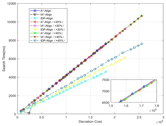
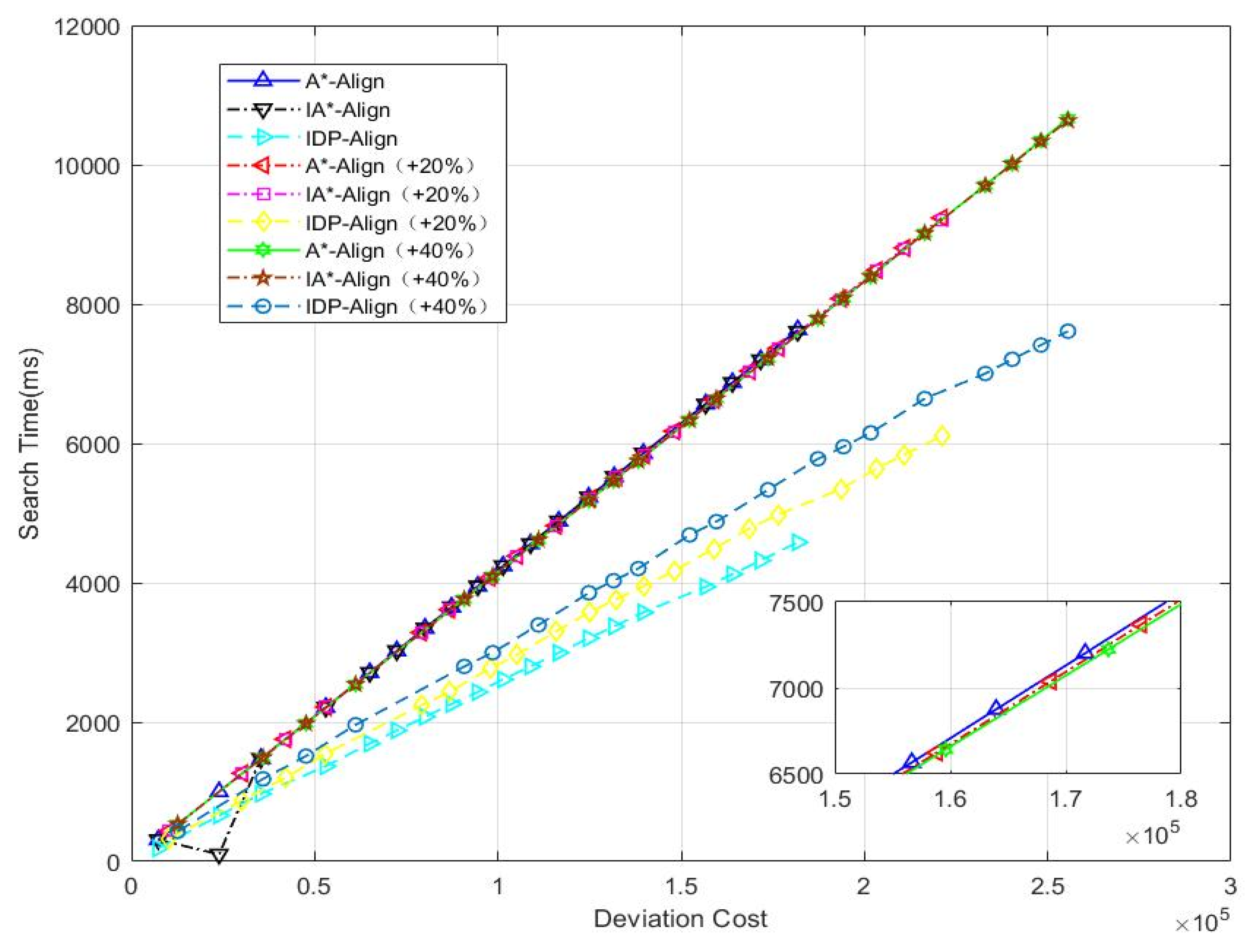
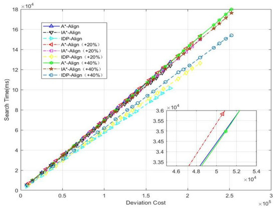
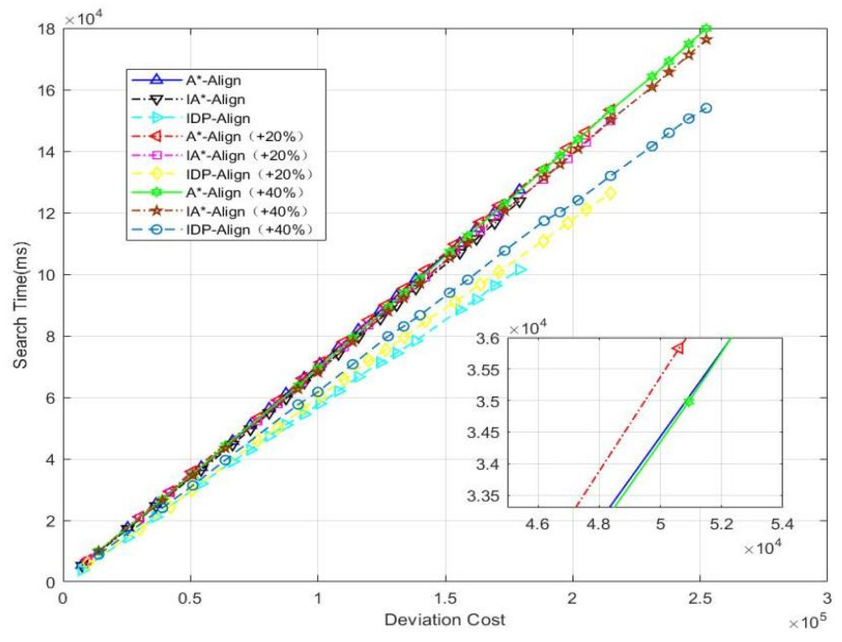
The data set $D_{B1}$ was constructed by Domestic Declarations and the given process model, as shown in Figure 20a. Then, 20% and 40% noise were added to the initial event log to produce two new data sets, denoted as D_B1+20% and D_B1+40%. $A^{\ast }-Align$, $OI{A}^{\ast }-Align$ and $IDP-Align$ were used to search the optimal alignment set (in Figure 21). Cost and search time were evaluated, and the proportion of fitted alignments in $D_{B1}$, D_B1 and D_B1+20% and D_B1+40% was extremely low. Thus, the search time was shortened only by 0.34%, 0.28% and 0.25% using $OI{A}^{\ast }-Align$ compared to $A^{\ast }-Align$. The certain proportion of alignments in $D_{B1}$, D_B1+20% and D_B1+40% were partially compared. Thus, the search time was reduced using $IDP-Align$ by 40%, 34% and 29% compared with $A^{\ast }-Align$. The noise was greater and the reduction of search time was smaller in the same data set. Fewer elements were automatically eliminated due to the initial deviation of some noise alignments occurring at the end. The difference of search time between $OI{A}^{\ast }-Align$ and $A^{\ast }-Align$ in $D_{B1}$, D_B1+20% and D_B1+40% are depicted in Figure 21 (partially enlarged).

Figure 21. Running result of $D_{B1}$, D_B1+20% and D_B1+40%.

The data set $D_{B2}$ was constructed by Domestic Declarations and the given process model, as shown in Figure 20b. Then, 20% and 40% noise were added to the initial event log to produce two new data sets, denoted as $D_{B2+20\%}$ and $D_{B2+40\%}$. The search time was shortened by 2.82%, 2.34% and 2% using $OI{A}^{\ast }-Align$ compared to $A^{\ast }-Align$. It could be seen that the ratio of fitted alignments in Figure 22 was larger than that in Figure 21. The search time was reduced using $IDP-Align$ by 20%, 18% and 14% compared with $A^{\ast }-Align$. The result showed that the improvement in Figure 22 was lower than that in Figure 21 due to the size of the data sets.

Figure 22. Running result of $D_{B2}$, D_B2+20% and D_B2+40%.

Table 7 records the time and cost obtained using $A^{\ast }-Align$, $I{A}^{\ast }-Align$ and $IDP-Align$. From Table 7, the search time of $IDP-Align$ was the least in the same data set compared with others.

Table 7. The experiment results of BPIC2020.

Method	A*-Align		IA*-Align		IDP-Align
Parameter	Time (ms)	Cost	Time (ms)	Cost	Time (ms)	Cost
D1	7632 ms	181,798	7606 ms	181,798	4582 ms	181,798
D1 (+20%)	9238 ms	221,042	9212 ms	221,042	6105 ms	221,042
D1 (+40%)	10,661 ms	255,518	10,635 ms	255,518	7611 ms	255,518
D2	127,340 ms	179,125	123,753 ms	179,125	101,475 ms	179,125
D2 (+20%)	153,426 ms	214,887	149,839 ms	214,887	126,275 ms	214,887
D2 (+40%)	179,863 ms	252,393	176,276 ms	252,393	153,998 ms	252,393

Table 8 lists all the numerical time differences in different data sets. From Table 8, we can find that the difference between $A^{\ast }-Align$ and $I{A}^{\ast }-Align$ was much smaller than the others. At the same time, we can also see the following two problems according to the time difference: (1) the time differences were basically proportional to the size of the data set; (2) noise addition has little effect on the time savings of $IDP-Align$.

Table 8. The numerical differences of experiment results.

Method	IA*-Align Is Subtracted by A*-Align	IDP-Align Is Subtracted by A*-Align	IDP-Align Is Subtracted by IA*-Align
Parameter	Time Difference Value (ms)	Time Difference Value (ms)	Time Difference Value (ms)
D1	26 ms	3050 ms	3024 ms
D1 (+20%)	26 ms	3133 ms	3107 ms
D1 (+40%)	26 ms	3050 ms	3024 ms
D2	3587 ms	25,865 ms	22,278 ms
D2 (+20%)	3587 ms	27,151 ms	23,564 ms
D2 (+40%)	3587 ms	25,865 ms	22,278 ms

5.4. Performance Comparison

The efficiency improvement of $IDP-Align$ was verified by the above experiments compared with the existing $A^{\ast }-Align$ and $I{A}^{\ast }-Align$. Moreover, the search time was effectively shortened on the premise of ensuring the minimum cost. However, the main performance of conformance checking was evaluated by taking cost, time, perspective, form and application range into account. Therefore, these features are discussed in Table 9.

Table 9. Check performances of various methods.

References	Cost	Time	Check Perspective	Check Form	Application Region
[13,19,33]	Minimum	$\to$	Control flow	static state	$\{L\cup M\}=D$
[42]	Minimum	$\downarrow$	Control flow	static state	$\{L\cup M\}=D$
[28]	Minimum	$\to$	Multi-perspective	static state	$\{L\cup M\}=D$
[29]	Minimum		Stochastic perspective	static state	$\{L\cup M\}=D$
[31,32]	Minimum	$\to$	Control flow	dynamic state	$\{L\cup M\}=D$
[39]	Minimum	$\downarrow$> [42]	Control flow	static state	$\{L\cup M\}=D$
This work	Minimum	$\downarrow$> [42]	Control flow	static state	$\{L\cup (M\backslash {\phi }_{pM}^{\ast })\}=D$

Note: $\to$ and $\downarrow$ represent the invariability and decline in search time, respectively. $\{L\cup M\}=D$ represents an arbitrary data set consisting of the event log and the initial model. $\{L\cup (M\backslash {\phi }_{pM}^{\ast })\}=D$ indicates the initial model in the data set not containing non-perceivable region.

6. Conclusions

The effective search for the optimal alignment is introduced in this paper, aiming at unweighted business processes with uniform unit cost. The search for the optimal alignment is efficiently improved compared with the traditional brute force search when dealing with a complex business process. The perceptible search mainly includes the following three steps: (i) According to the behavior characteristics of different substructures in the process model, the perceptible region is determined by reverse search. The location of the initial deviation is inversely proportional to the number of deviations when the initial deviation occurs in the perceptible region. (ii) The recorded location of the initial deviation is firstly set to 0. The recorded location is updated when the location of the current initial deviation is greater than the previously recorded value. At the same time, its recorded location is used as the optimal metric of the same trace. (iii) The recorded location is unchanged and the comparison of alignment is automatically terminated as non-optimal when the location of the current initial deviation is smaller than the previously recorded value. In summary, the search workload of the optimal alignment can be effectively reduced now that some alignments are only partially compared based on the perception of the initial deviation.

References

- Li, C.; Ge, J.; Huang, L.; Hu, H.; Wu, B.; Yang, H.; Hu, H.; Luo, B. Process mining with token carried data. Inf. Sci. 2016, 328, 558–576. [Google Scholar] [CrossRef] [Scilit]
- Caldeira, J.; Abreu, F.B.e. Software development process mining: Discovery, conformance checking and enhancement. In Proceedings of the 2016 10th International Conference on the Quality of Information and Communications Technology (QUATIC), Lisbon, Portugal, 6–9 September 2016; pp. 254–259. [Google Scholar]
- Van der Aalst, W.; Weijters, T.; Maruster, L. Workflow mining: Discovering process models from event logs. IEEE Trans. Knowl. Data Eng. 2004, 16, 1128–1142. [Google Scholar] [CrossRef] [Scilit]
- Weidlich, M.; Mendling, J. Perceived consistency between process models. Inf. Syst. 2012, 37, 80–98. [Google Scholar] [CrossRef] [Scilit]
- Alizadeh, M.; Lu, X.; Fahland, D.; Zannone, N.; van der Aalst, W.M. Linking data and process perspectives for conformance analysis. Comput. Secur. 2018, 73, 172–193. [Google Scholar] [CrossRef] [Scilit]
- van Zelst, S.J.; van Dongen, B.F.; van der Aalst, W.M. Event stream-based process discovery using abstract representations. Knowl. Inf. Syst. 2018, 54, 407–435. [Google Scholar] [CrossRef] [Scilit]
- Pourmasoumi, A.; Kahani, M.; Bagheri, E. Mining variable fragments from process event logs. Inf. Syst. Front. 2017, 19, 1423–1443. [Google Scholar] [CrossRef] [Scilit]
- Buijs, J.C.; La Rosa, M.; Reijers, H.A.; van Dongen, B.F.; van der Aalst, W.M. Improving business process models using observed behavior. In Proceedings of the 2nd International Symposium on Data-Driven Process Discovery and Analysis (SIMPDA), Campione d’Italia, Italy, 18–20 June 2012; pp. 44–59. [Google Scholar]
- Qi, H.; Du, Y.; Qi, L.; Wang, L. An approach to repair Petri net-based process models with choice structures. Enterp. Inf. Syst. 2018, 12, 1149–1179. [Google Scholar] [CrossRef] [Scilit]
- Zhang, L.; Fang, X.; Shao, C.; Wang, L. Real-time repair of business processes based on alternative operations in case of uncertainty. IEEE Access 2021, 9, 23672–23690. [Google Scholar] [CrossRef] [Scilit]
- Kleiner, N. Delta analysis with workflow logs: Aligning business process prescriptions and their reality. Requir. Eng. 2005, 10, 212–222. [Google Scholar] [CrossRef] [Scilit]
- Garcia-Banuelos, L.; van Beest, N.R.; Dumas, M.; La Rosa, M.; Mertens, W. Complete and interpretable conformance checking of business processes. IEEE Trans. Softw. Eng. 2017, 44, 262–290. [Google Scholar] [CrossRef] [Scilit]
- van der Aalst, W.; Adriansyah, A.; van Dongen, B. Replaying history on process models for conformance checking and performance analysis. Wiley Interdiscip. Rev. Data Min. Knowl. Discov. 2012, 2, 182–192. [Google Scholar] [CrossRef] [Scilit]
- Fang, X.; Cao, R.; Liu, X.; Wang, L. A method of mining hidden transition of business process based on region. IEEE Access 2018, 6, 25543–25550. [Google Scholar] [CrossRef] [Scilit]
- Armas-Cervantes, A.; Baldan, P.; Dumas, M.; Garcia-Bañuelos, L. Diagnosing behavioral differences between business process models: An approach based on event structures. Inf. Syst. 2016, 56, 304–325. [Google Scholar] [CrossRef] [Scilit]
- Fahland, D.; Van Der Aalst, W.M. Model repair-aligning process models to reality. Inf. Syst. 2015, 47, 220–243. [Google Scholar] [CrossRef] [Scilit]
- Bauer, M.; Van der Aa, H.; Weidlich, M. Estimating process conformance by trace sampling and result approximation. In Proceedings of the Business Process Management: 17th International Conference, BPM 2019, Proceedings 17, Vienna, Austria, 1–6 September 2019; Springer International Publishing: Cham, Switzerland, 2019. [Google Scholar]
- De Leoni, M.; Maggi, F.M.; van der Aalst, W.M. Aligning event logs and declarative process models for conformance checking. In Proceedings of the Business Process Management: 10th International Conference, BPM 2012, Proceedings 10, Tallinn, Estonia, 3–6 September 2012; Springer: Berlin/Heidelberg, Germany, 2012; pp. 82–97. [Google Scholar]
- Adriansyah, A.; van Dongen, B.F.; van der Aalst, W.M. Conformance checking using cost-based fitness analysis. In Proceedings of the 2011 IEEE 15th International Enterprise Distributed Object Computing Conference, Helsinki, Finland, 29 August–2 September 2011; pp. 55–64. [Google Scholar]
- Leemans, S.J.; Fahland, D.; Van Der Aalst, W.M. Discovering block-structured process models from event logs-a constructive approach. In Proceedings of the Application and Theory of Petri Nets and Concurrency: 34th International Conference, PETRI NETS 2013, Proceedings 34, Milan, Italy, 24–28 June 2013; Springer: Berlin/Heidelberg, Germany, 2013; pp. 311–329. [Google Scholar]
- Buijs, J.C.; Van Dongen, B.F.; van Der Aalst, W.M. On the role of fitness, precision, generalization and simplicity in process discovery. In Proceedings of the On the Move to Meaningful Internet Systems: OTM 2012: Confederated International Conferences: CoopIS, DOA-SVI, and ODBASE 2012, Proceedings, Part I, Rome, Italy, 10–14 September 2012; Springer: Berlin/Heidelberg, Germany, 2012; pp. 305–322. [Google Scholar]
- de Leoni, M.; Maggi, F.M.; van der Aalst, W.M. An alignment-based framework to check the conformance of declarative process models and to preprocess event-log data. Inf. Syst. 2015, 47, 258–277. [Google Scholar] [CrossRef] [Scilit]
- Jagadeesh Chandra Bose, R.P.; van der Aalst, W. Trace alignment in process mining: Opportunities for process diagnostics. In Proceedings of the International Conference on Business Process Management, Hoboken, NJ, USA, 13–16 September 2010; Springer: Berlin/Heidelberg, Germany, 2010; pp. 227–242. [Google Scholar]
- Weidlich, M.; Polyvyanyy, A.; Desai, N.; Mendling, J. Process compliance measurement based on behavioural profiles. In Proceedings of the Advanced Information Systems Engineering: 22nd International Conference, CAiSE 2010, Proceedings 22, Hammamet, Tunisia, 7–9 June 2010; Springer: Berlin/Heidelberg, Germany, 2010; pp. 499–514. [Google Scholar]
- Bogdanov, E.; Cohen, I.; Gal, A. Conformance checking over stochastically known logs. In Proceedings of the International Conference on Business Process Management, Münster, Germany, 11–16 September 2022; Springer International Publishing: Cham, Switzerland, 2022; pp. 105–119. [Google Scholar]
- Pegoraro, M.; Uysal, M.S.; van der Aalst, W.M. Conformance checking over uncertain event data. Inf. Syst. 2021, 102, 101810. [Google Scholar] [CrossRef] [Scilit]
- Calheno, R.; Carvalho, P.; Lima, S.R.; Henriques, P.R.; Merino, M.R. Improving conformance checking in process modelling: A multiperspective algorithm. J. Super-Comput. 2023, 79, 18256–18292. [Google Scholar] [CrossRef] [Scilit]
- Felli, P.; Gianola, A.; Montali, M.; Rivkin, A.; Winkler, S. Multi-perspective conformance checking of uncertain process traces: An SMT-based approach. Eng. Appl. Artif. Intell. 2023, 126, 106895. [Google Scholar] [CrossRef] [Scilit]
- Leemans, S.J.; van der Aalst, W.M.; Brockhoff, T.; Polyvyanyy, A. Stochastic process mining: Earth movers’ stochastic conformance. Inf. Syst. 2021, 102, 101724. [Google Scholar] [CrossRef] [Scilit]
- Wang, L.; Du, Y.; Qi, M.; Qi, H.; He, Z. Petri net-based deviation detection between a process model with loop semantics and event logs. Concurr. Comput. Pract. Exp. 2018, 30, e4419. [Google Scholar] [CrossRef] [Scilit]
- van Zelst, S.J.; Bolt, A.; Hassani, M.; van Dongen, B.F.; van der Aalst, W.M.P. Online conformance checking: Relating event streams to process models using prefix-alignments. Int. J. Data Sci. Anal. 2019, 8, 269–284. [Google Scholar] [CrossRef] [Scilit]
- Lee, W.L.J.; Burattin, A.; Munoz-Gama, J.; Sepúlveda, M. Orientation and conformance: A HMM-based approach to online conformance checking. Inf. Syst. 2021, 102, 101674. [Google Scholar] [CrossRef] [Scilit]
- Adriansyah, A.; Van Dongen, B.F.; van der Aalst, W.M. Cost-based conformance checking using the A* Algorithm. BPM Cent. Rep. BPM-11-11 BPMcenter.Org 2011, 1111, 1–14. [Google Scholar]
- Adriansyah, A.; van Dongen, B.F.; van der Aalst, W.M. Towards robust conformance checking. In Proceedings of the Business Process Management Workshops: BPM 2010 International Workshops and Education Track, Revised Selected Papers 8, Hoboken, NJ, USA, 13–15 September 2010; Springer: Berlin/Heidelberg, Germany, 2010; pp. 122–133. [Google Scholar]
- De Weerdt, J.; De Backer, M.; Vanthienen, J.; Baesens, B. A robust F-measure for evaluating discovered process models. In Proceedings of the 2011 IEEE Symposium on Computational Intelligence and Data Mining (CIDM), Paris, France, 11–15 April 2011; pp. 148–155. [Google Scholar]
- Bloemen, V.; van Zelst, S.J.; van der Aalst, W.M.; van Dongen, B.F.; van de Pol, J. Maximizing synchronization for aligning observed and modelled behaviour. In Proceedings of the Business Process Management: 16th International Conference, BPM 2018, Proceedings 16, Sydney, NSW, Australia, 9–14 September 2018; Springer International Publishing: Cham, Switzerland, 2018; pp. 233–249. [Google Scholar]
- Reißner, D.; Armas-Cervantes, A.; Conforti, R.; Dumas, M.; Fahland, D.; La Rosa, M. Scalable alignment of process models and event logs: An approach based on automata and s-components. Inf. Syst. 2020, 94, 101561. [Google Scholar] [CrossRef] [Scilit]
- Lee, W.L.; Verbeek, H.M.; Munoz-Gama, J.; van der Aalst, W.M.; Sepúlveda, M. Recomposing conformance: Closing the circle on decomposed alignment-based conformance checking in process mining. Inf. Sci. 2018, 466, 55–91. [Google Scholar] [CrossRef] [Scilit]
- Song, W.; Xia, X.; Jacobsen, H.-A.; Zhang, P.; Hu, H. Efficient alignment between event logs and process models. IEEE Trans. Serv. Comput. 2016, 10, 136–149. [Google Scholar] [CrossRef] [Scilit]
- Dumas, M.; García-Bañuelos, L. Process mining reloaded: Event structures as a unified representation of process models and event logs. In Proceedings of the Application and Theory of Petri Nets and Concurrency: 36th International Conference, PETRI NETS 2015, Proceedings 36, Brussels, Belgium, 21–26 June 2015; Springer International Publishing: Cham, Switzerland, 2015; pp. 33–48. [Google Scholar]
- Zhong, C.; Zhang, H.; Huang, H.; Chen, Z.; Li, C.; Liu, X.; Li, S. DOMICO: Checking conformance between domain models and implementations. Softw. Pract. Exp. 2024, 54, 595–616. [Google Scholar] [CrossRef] [Scilit]
- Zhang, L.; Fang, X. Business process fitness analysis based on alignment processing and deviation detection. Comput. Integr. Manuf. Syst. 2020, 26, 1573–1581. [Google Scholar]
Disclaimer/Publisher’s Note: The statements, opinions and data contained in all publications are solely those of the individual author(s) and contributor(s) and not of MDPI and/or the editor(s). MDPI and/or the editor(s) disclaim responsibility for any injury to people or property resulting from any ideas, methods, instructions or products referred to in the content. |
© 2024 by the authors. Licensee MDPI, Basel, Switzerland. This article is an open access article distributed under the terms and conditions of the Creative Commons Attribution (CC BY) license (https://creativecommons.org/licenses/by/4.0/).