


Abstract
High-precision sediment distribution maps are indispensable for nearshore sediment dynamics and ecology and nearshore resource management. Using grain-size data of surface sediments from the nearshore waters of Lianyungang and auxiliary datasets including bathymetric and hydrodynamic conditions, this study assessed Random Forest (RF), eXtreme Gradient Boosting (XGBoost), and Support Vector Regression (SVR) for predicting sediment grain-size fractions and mapping sediment substrate types. All three models capture the spatial gradient of sediment grain size from fine to coarse from the nearshore to the offshore regions, but differ in preserving local heterogeneity and defining transition boundaries: XGBoost delivers the most balanced performance by preserving grain-size variability, reducing boundary mixing, and improving the identification of classes with limited samples; RF excels in robust delineation of gradual transitions, whereas SVR tends to produce fragmented boundaries and unstable performance for classes with limited samples. Feature importance reveals that hydrodynamic drivers dominate the spatial distribution of sand, whereas terrain indices are more influential for the clay distribution pattern, confirming the role of microtopography in modulating fine-sediment trapping. Overall, this study improves mapping accuracy and supports marine spatial planning and coastal infrastructure design.
1. Introduction
Coastal ecosystems are increasingly subjected to intensifying anthropogenic and natural pressures, driven by human activities and land–sea coupling processes. These cumulative stressors pose significant threats to ecosystem integrity and function [1]. In this context, marine spatial planning (MSP) relies critically on robust, high-resolution ecological and environmental baselines to inform zoning designations, regulatory frameworks, and sustainable-use decisions [2]. Among such foundational datasets, high-accuracy seabed substrate maps constitute an essential component. Such maps serve not only as a primary basis for characterizing benthic habitat heterogeneity but also as a key tool for predicting the spatial distribution of marine biota in coastal waters. Substrate grain size functions as a proximal environmental driver that strongly correlates with benthic biodiversity patterns [3]. Moreover, distinct substrate types exhibit characteristic surface roughness and microtopographic properties, which jointly modulate habitat suitability, refuge availability, and ecological connectivity for benthic organisms [4]. Consequently, seabed substrate maps support both species distribution inference and broader biodiversity assessments, providing a scientific basis for MSP as well as conservation and restoration actions.
Conventional nearshore seabed substrate mapping typically relies on field sampling combined with geostatistical interpolation, most notably ordinary kriging and cokriging, which explicitly model spatial autocorrelation [5,6]. While historically valuable, these methods face three fundamental limitations. First, their predictive reliability is contingent upon strong assumptions of stationarity and isotropic spatial autocorrelation, necessitating dense, spatially balanced sampling; prediction uncertainty escalates markedly in data-sparse regions. Second, their linear or semi-linear functional forms constrain their capacity to represent complex, nonlinear interactions between sedimentary patterns and multivariate environmental covariates (e.g., hydrodynamic energy, bathymetric gradients, and sediment transport pathways). Third, inherent smoothing effects degrade resolution and bias predictions toward dominant substrate classes, particularly undermining accuracy for rare substrates and small-sample scenarios [7,8]. As marine environmental research increasingly requires higher spatial fidelity and thematic precision, these constraints make conventional approaches inadequate for high-resolution substrate mapping and highlight the need for more flexible, data-adaptive alternatives.
Machine learning (ML) methods have emerged as powerful tools for the spatial prediction of environmental variables, owing to their capacity to model nonlinear relationships, integrate heterogeneous data sources, and maintain robust performance even with limited training samples [6]. Relative to classical statistical and geostatistical models, ML algorithms impose fewer distributional and structural assumptions, enabling them to learn complex, multidimensional associations between environmental drivers (e.g., bathymetry, slope, current velocity, wave energy) and sediment properties directly from empirical data [9,10,11]. Furthermore, many ML frameworks, including tree-based ensembles and kernel-based regressors, provide interpretable feature importance metrics that help quantify the influence of environmental controls on substrate distribution [12]. This dual advantage of improved predictive accuracy and process interpretability makes ML methods well suited for higher fidelity substrate mapping with broader applicability and stronger mechanistic grounding. For instance, Stephens et al. [9] demonstrated that incorporating terrain and hydrodynamic covariates into Random Forest (RF) improves sediment prediction accuracy. Lark et al. [6] reported substantial gains in RF-based sediment-type mapping by integrating ocean dynamic variables. Pham et al. [13] used eXtreme Gradient Boosting (XGBoost) to fuse remote sensing and in situ data and improved model generalization in topographically complex nearshore settings. Similarly, Support Vector Regression (SVR), with kernel-based nonlinear mapping capability, has shown promise in quantitative sediment modeling. Wang et al. [14] successfully predicted seabed acoustic attenuation coefficients using SVR trained on sediment grain-size parameters, underscoring its viability for continuous sediment property estimation.
Despite growing empirical success of RF, XGBoost, and SVR in terrestrial and broad-scale marine environmental mapping, their application to nearshore seabed substrate prediction remains nascent and fragmented. Compared with the extensive literature on ML-driven soil mapping [15], studies targeting nearshore sediments remain limited and are often confined to localized depositional settings, such as estuaries [16] and embayments [17], with limited cross-environmental validation. Moreover, existing work has largely emphasized categorical classification rather than continuous prediction of sediment grain-size fractions (e.g., clay, silt, sand percentages), which limits the usefulness of ML outputs for sediment transport modeling, geochemical analysis, and fine-scale habitat assessment. Finally, methodological comparisons remain rare: most studies apply a single ML algorithm in isolation [18,19], and systematic benchmarking of RF, XGBoost, and SVR under a consistent preprocessing pipeline, identical covariate, and a unified validation framework is still lacking for nearshore substrate mapping. This gap impedes evidence-based selection of optimal algorithms across contrasting hydrodynamic regimes and geomorphic contexts.
To bridge these gaps, this study pursues three interrelated objectives: (i) to compare RF, XGBoost, and SVR for the continuous prediction of clay, silt, and sand fractions in nearshore surface sediments under standardized preprocessing, hyperparameter tuning, and cross-validation; (ii) to generate substrate-type maps by classifying predicted sediment grain-size fractions using the Folk sediment classification scheme and to evaluate classification accuracy against independent observations; and (iii) to interpret the relative contributions of environmental covariates, particularly hydrodynamic and topographic variables, using model-agnostic interpretability analysis.
2. Data and Methods
2.1. Study Area
The study area is situated in the nearshore waters off northeastern Jiangsu Province, China, bounded by Rizhao City (Shandong Province) to the north, the abandoned Yellow River Delta of northern Jiangsu to the south, and the South Yellow Sea to the east. Tectonically, it occupies a critical transition zone between the Sulu-Lu uplift and the northern Jiangsu depression, and its structural framework is governed by two dominant fault systems, oriented northeast and northwest, that originated during the Yanshanian orogeny. The coastline exhibits marked segmentation: in the northern sector, it trends northeast–southwest; in the southern sector, it trends northwest–southeast, collectively forming an open embayment system. Notably, the nearshore waters off Lianyungang are hydrologically connected to the northern flank of the abandoned Yellow River Delta, with paleo-Yellow River sediment inputs exerting a profound influence on the depositional environment. Consequently, surface sediments in the study area are dominated by deltaic deposits, with silt as the primary grain-size component, displaying a characteristic offshoreward coarsening trend (finer sediments nearshore and coarser sediments offshore) [20]. Legacy sediment supply has formed a thick silt–mud depocenter in the bay, with sediment thickness exceeding 10 m near the Guanhe estuary and reaching about 5–8 m toward the bay head. The regional topography slopes gently from southwest to northeast, encompassing diverse nearshore geomorphic units. The subaqueous morphology can be broadly described by subaqueous shoals, relict sand plains occurring at water depths of 10–27 m with residual fine-sand cover, and palaeochannels or shelf valleys that are about 1–1.5 km wide and contain locally deep pools deeper than 20 m.
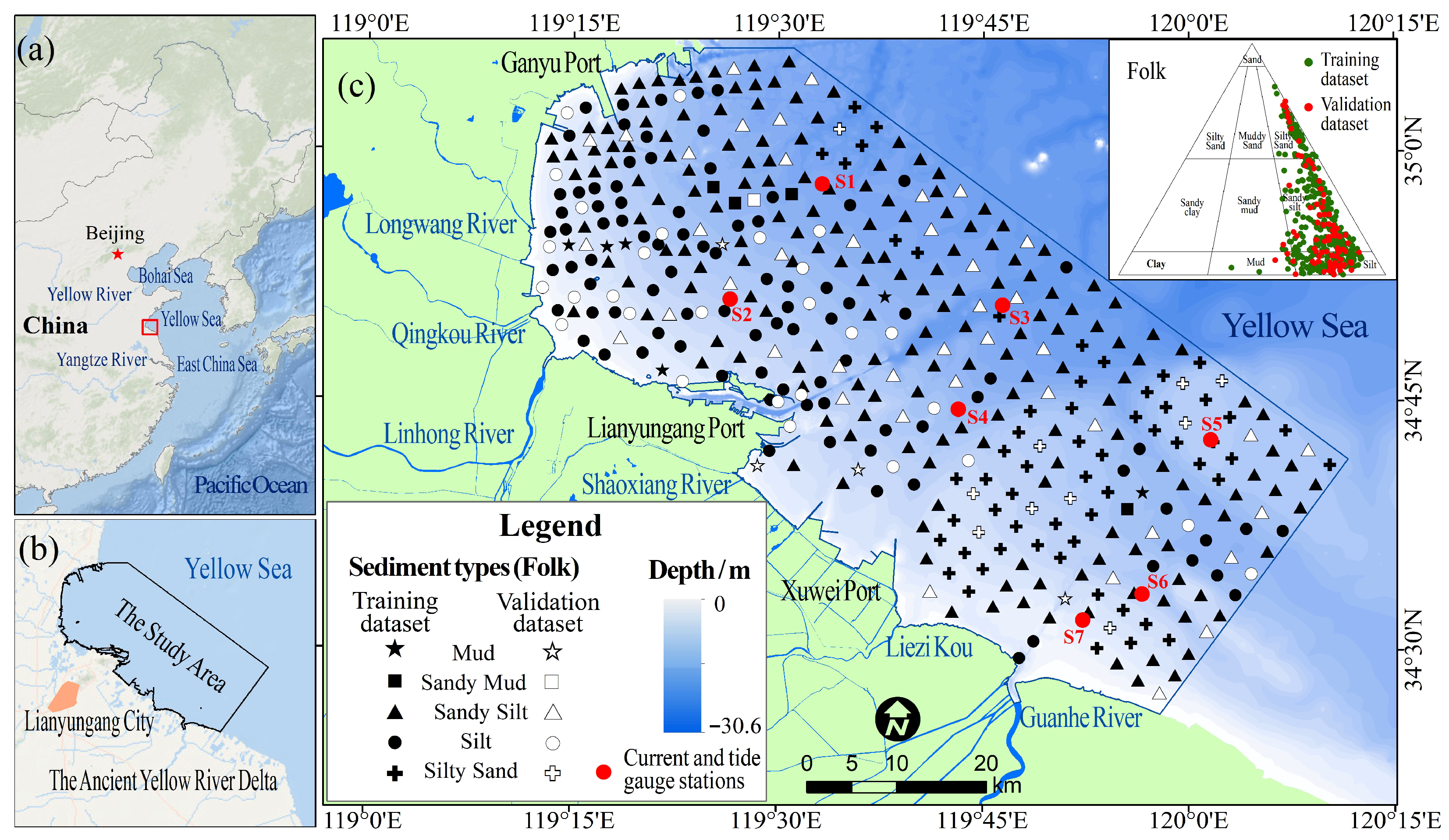
Tidal and wave processes constitute the primary hydrodynamic drivers governing sediment transport and morphodynamic evolution in this region. The tidal regime is characterized as a regular semidiurnal type, with a mean tidal range of 3.08–3.34 m and a maximum recorded range of 5.5 m. The averaged tidal current velocities range from 40 to 50 cm/s, while peak flood and ebb velocities reach up to 67 cm/s. Nearshore currents predominantly exhibit reciprocating behavior, whereas offshore currents are primarily rotary, with flood currents consistently stronger than ebb currents [21]. A distinct latitudinal gradient in current velocity is observed, increasing from north to south; during flood tide, mean current velocities in offshore waters between Xuwei Port and the Guanhe River mouth can attain 0.36–0.87 m/s. The geographical location of the study area and distribution of sampling stations are illustrated in Figure 1.
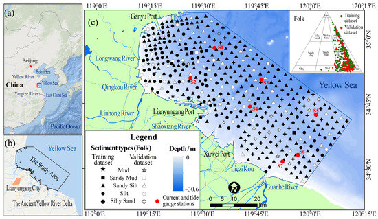
Figure 1.
Location of the study area and sampling stations. (a) Location of the study region in China. (b) Outline of the study area in the Yellow Sea near Lianyungang City and the ancient Yellow River Delta. (c) Bathymetry and distribution of training/validation samples by Folk sediment types; red dots mark current and tide gauge stations. Inset: Folk ternary diagram.
2.2. Data
2.2.1. Sediment Sampling and Grain-Size Data Processing
Sediment sampling was conducted across the study area from late August to early October 2020, using a systematic 3 km × 3 km grid design to ensure spatial representativeness. Sediment samples were collected using a Van Veen grab sampler, and undisturbed surface sediments (0–5 cm) were subsampled, sealed in pre-cleaned polyethylene bags, and stored at 4 °C pending laboratory analysis. Each sample was uniquely labeled in chronological order of collection (HZW001–HZW427), and precise geographic coordinates (latitude and longitude) were recorded in situ using a differential GPS receiver. Due to operational constraints, such as aquaculture infrastructure and restricted access in port zones, the actual locations of some sampling sites deviated moderately from the pre-defined grid positions.
Prior to grain-size analysis, all samples were pretreated to remove organic matter and carbonate components, followed by dispersion to ensure particle separation. Grain-size distributions were determined using a Mastersizer 2000 laser diffraction particle-size analyzer (Malvern Instruments, Malvern, UK) [22], with measurements recorded at intervals of 0.25Φ. Based on the Udden–Wentworth grade scale [23], the grain-size spectra were categorized into three sedimentary fractions: sand (−1 to 4Φ), silt (4 to 8Φ), and clay (>8Φ). The proportional content of each fraction was expressed as a volume percentage. Sediment classification and nomenclature for each station were then performed according to the Folk classification scheme. The resulting classifications for all 427 samples are presented in the Folk ternary diagram in Figure 1.
Given that the sand–silt–clay percentages represent compositional data, which are subject to non-negativity and constant sum constraints, direct statistical modeling may introduce closure effects and spurious correlations among components [24]. To mitigate the closure problem and improve the statistical properties of the dataset, the three-component percentage data were transformed using the additive log-ratio (alr) transformation, following established methodologies [25,26].
The inverse transformation is given by
where xi represents the volume percentage of the ith sediment grain-size fraction, alri denotes the transformed value after additive log-ratio (alr) transformation, and p is the number of sediment components.
Based on the transformation in Equation (1), alrcs corresponds to the base- logarithm of the clay-to-silt ratio (), and alrss to the base- logarithm of the sand-to-silt ratio ().
Since compositional data containing zero values are incompatible with logarithmic transformation [27], any zero percentages in the grain-size fractions were replaced by the analytical detection limit of the laser particle-size analyzer (0.001%) prior to transformation.
To evaluate the generalization capability of the machine learning models, the dataset was partitioned into training and validation subsets. Using the Subset Features tool in ArcGIS, 85 stations (approximately 20% of the total samples) were randomly selected to form the independent validation set. The remaining 342 stations (approximately 80%) constituted the training set used for model development.
2.2.2. Environmental Covariates
To characterize the physical controls on nearshore sediment distribution, this study integrates three complementary categories of environmental covariates: (i) terrain-derived geomorphic descriptors, (ii) numerically simulated hydrodynamic variables, and (iii) a spatial distance metric reflecting land–sea gradients. Terrain parameters capture static seabed morphology and its influence on flow routing and sediment trapping; hydrodynamic variables represent the dynamic forcing governing sediment transport, sorting, and deposition; and distance to coastline serves as a surrogate for gradients in terrestrial sediment supply, freshwater influence, and hydrodynamic energy decay. Together, these covariates provide a mechanistically grounded, multi-scale representation of depositional controls (Table 1).
Table 1.
Predictor variables used in RF, XGBoost and SVR models.
- (1)
- Terrain parameters
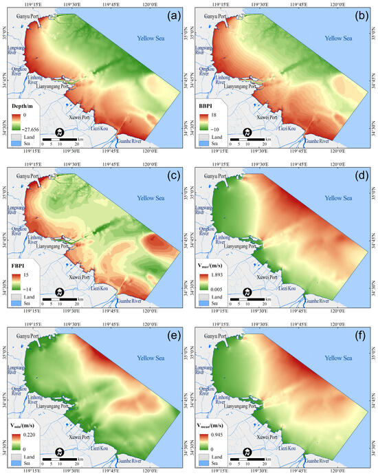
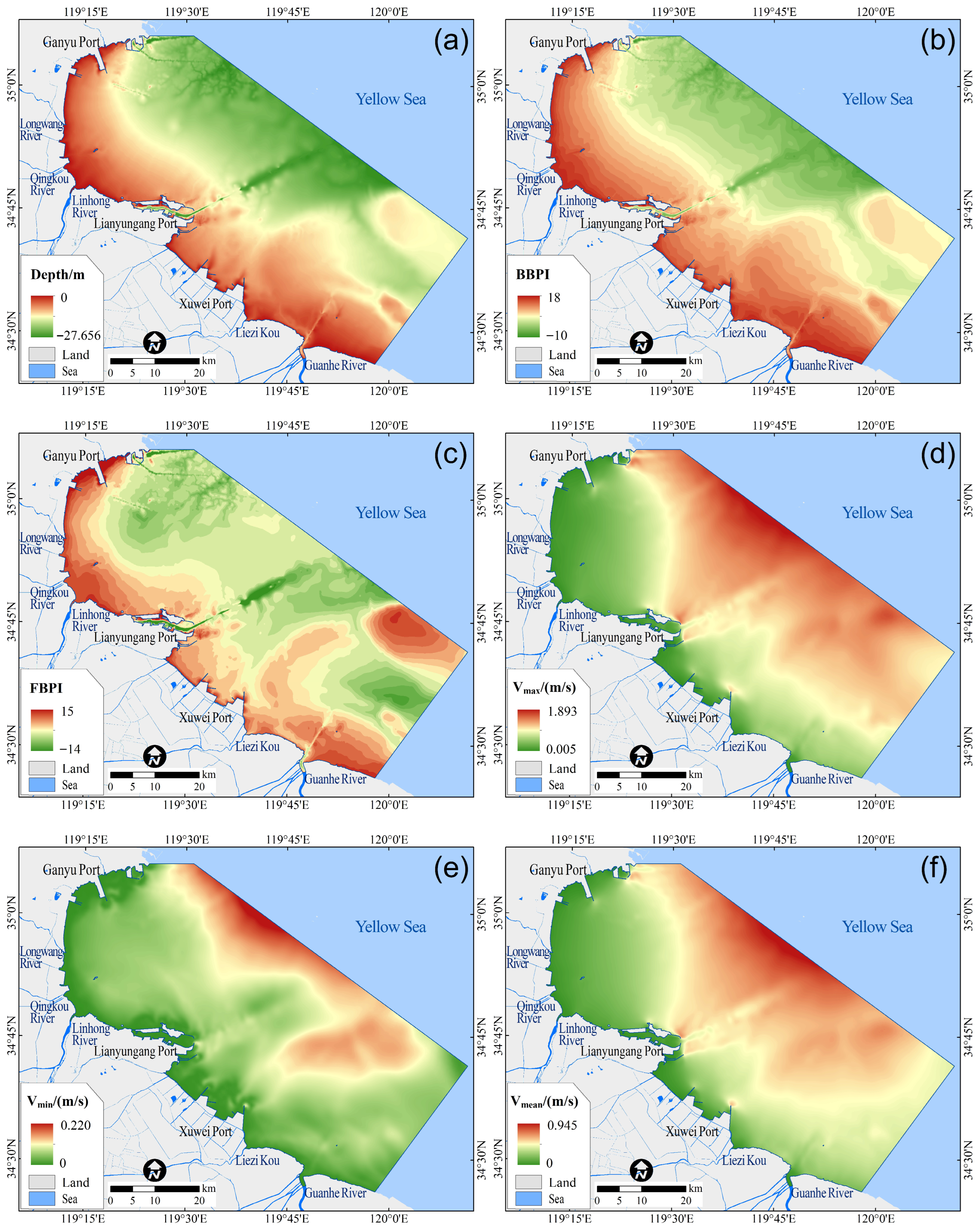
Terrain covariates include water depth (Depth), the broad-scale bathymetric position index (BBPI), and the fine-scale bathymetric position index (FBPI) (Figure 2a–c). Depth is the primary descriptor of bathymetry and serves as a foundational control on wave and current energy dissipation. BBPI and FBPI are terrain derivatives that quantify local relief relative to surrounding areas at distinct spatial scales. BBPI captures regional geomorphic positions, whereas FBPI resolves fine-scale microtopographic features, together characterizing seabed heterogeneity across multiple morphological scales.
Figure 2.
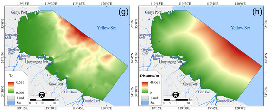
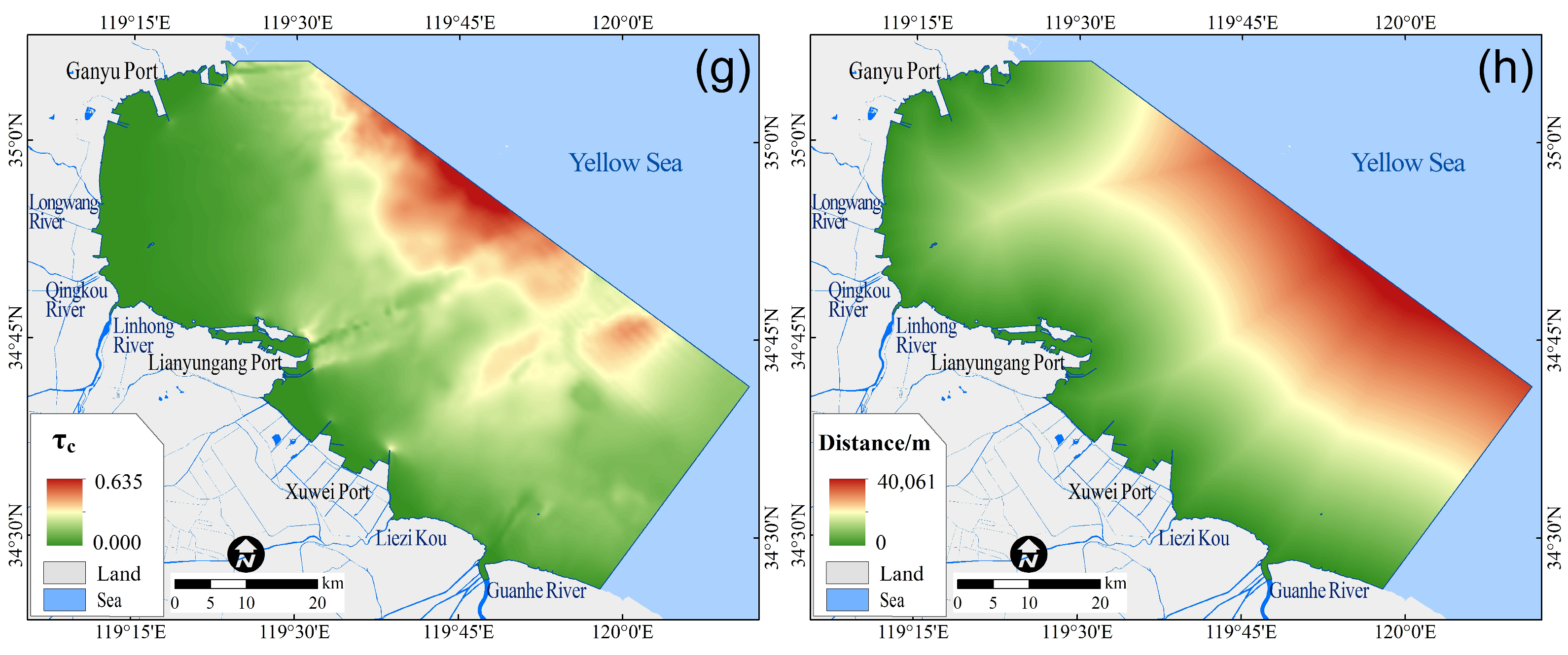
Spatial distribution of environmental covariates used for model development in the study area. (a) Water depth (Depth). (b) Large-scale bathymetric position index (BBPI). (c) Fine-scale bathymetric position index (FBPI). (d) Maximum tidal current velocity (Vmax). (e) Minimum tidal current velocity (Vmin). (f) Mean tidal current velocity (Vmean). (g) Current-induced bed shear stress (τc). (h) Distance to the coastline (Distance).
Water depth data were extracted from digitized nautical charts and interpolated in ArcGIS 10.8 using the Topo to Raster tool to generate a submarine digital elevation model (DEM) with a uniform raster resolution of 60 m. BBPI and FBPI were computed from this DEM using the Benthic Terrain Modeler (BTM) toolbox in ArcGIS [28]. BBPI was calculated with an inner radius of 300 m and outer radius of 3000 m to emphasize the regional-scale bathymetric context; FBPI employed an inner radius of 180 m and outer radius of 300 m to resolve localized topographic variability. This dual radius setup improves sensitivity to the target spatial scale and reduces edge-related artifacts and noise.
- (2)
- Hydrodynamic parameters
Hydrodynamic covariates include maximum (Vmax), minimum (Vmin), and mean (Vmean) tidal current velocities, as well as bed shear stress (τc) induced by near-bed currents (Figure 2d–g). Vmax, Vmin, and Vmean describe the magnitude and variability of tidal currents, which are key controls on sediment entrainment thresholds and transport capacity. τc quantifies the fluid shear stress exerted on the seabed, integrating the potential of currents to initiate motion, resuspend, and transport fine-grained sediments. It thus serves as a key link between hydrodynamic conditions and sedimentary processes.
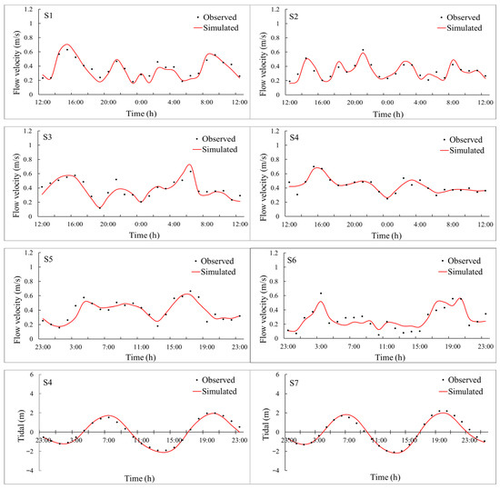
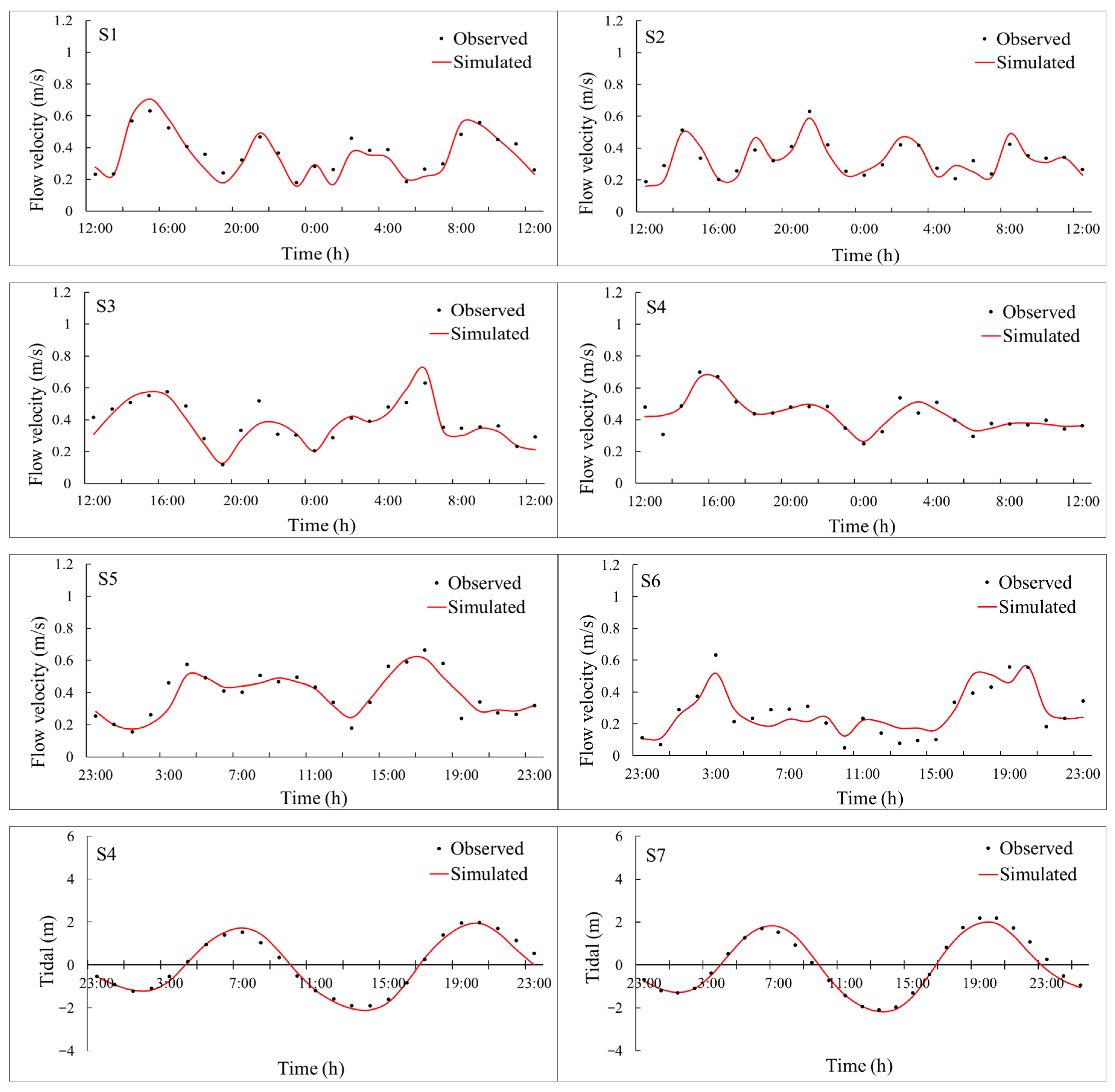
Hydrodynamic fields were simulated using the MIKE 21 HD module, configured with an unstructured triangular mesh optimized for coastal complexity. Bathymetry was prescribed from the 60 m resolution DEM described above. Open-boundary tidal conditions were specified using the FES2022b global tidal product (AVISO+) [29]. To ensure temporal congruence with field sampling, the simulation spanned 55 consecutive days from 20 August to 10 October 2020, fully encompassing the sediment collection period. Model performance was rigorously validated against in situ measurements: observed current velocity (ADCP moorings) and tidal elevation (pressure sensors) from seven independent stations within the domain were compared against corresponding model outputs (Figure 3; station locations in Figure 1). Time series comparisons between simulated and observed values (Figure 3) show close agreement in overall trends, confirming the model’s reliability. Following the simulation, the velocity field was extracted, and Vmax, Vmin, and Vmean were statistically derived for each grid cell within the study area. The bed shear stress τc was subsequently calculated from current velocity using a standard formulation [30]:
where is water density, with a value of 1.025 × 10³ kg/m3; Cd is the bottom drag coefficient, with a value of 3.1 × 10⁻³, and Vc is the depth average current velocity.
Figure 3.
Validation of MIKE 21 simulations against observations for current velocity (S1–S6) and tidal elevation (S4,S7) during an independent period on 27–28 November 2023. (S1–S4): The x-axis values represent 12:00 on 27 November to 12:00 on 28 November; (S5–S7): the x-axis values represent 23:00 on 27 November to 23:00 on 28 November.
All derived hydrodynamic rasters were resampled to 60 m resolution in ArcGIS and used directly as model covariates.
- (3)
- Distance to the coastline
Distance to the coastline (Distance) is a spatial explicit metric encoding the progressive attenuation of terrestrial influences from fluvial sediment delivery and freshwater discharge to wave energy refraction and wind-driven mixing as a function of offshore distance. It thus serves as a parsimonious yet physically meaningful proxy for land–sea coupling intensity and provides critical contextual information for interpreting spatial trends in sediment composition.
This variable was generated in ArcGIS 10.8 using the Euclidean Distance tool applied to a high-accuracy coastline vector dataset (derived from 2020 Sentinel-2 multispectral imagery). For each 60 m grid cell center within the study extent, the shortest orthogonal distance to the nearest shoreline segment was computed, yielding a continuous 60 m resolution raster surface (Figure 2h).
2.3. Machine Learning Methods
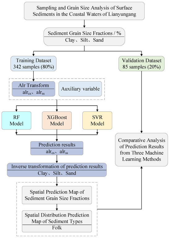
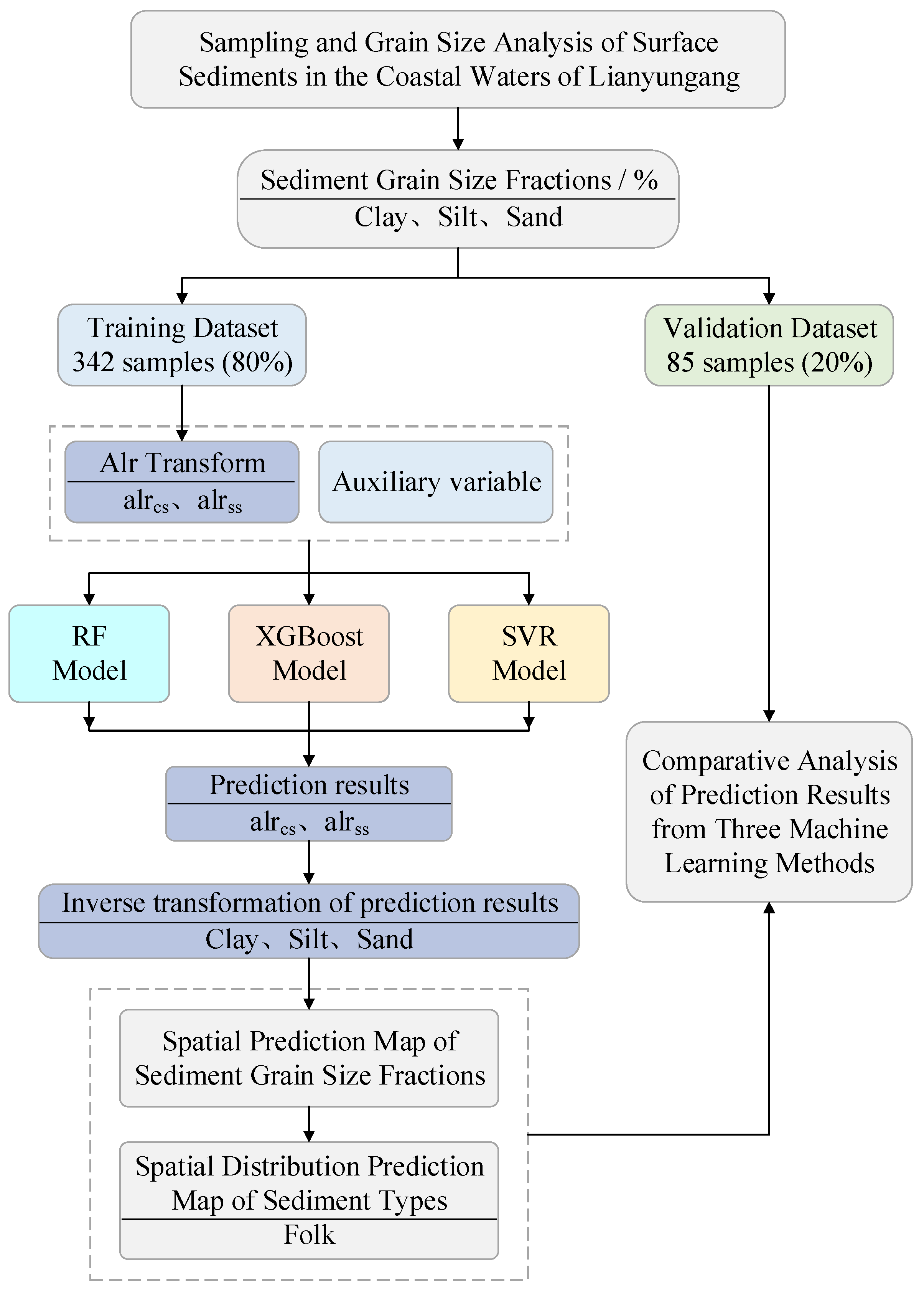
As summarized in Figure 4, using the additive log-ratio (alr)-transformed sediment grain-size fraction data (sand, silt, clay) described in Section 2.2.1, alongside spatially explicit raster covariate layers representing terrain morphology, hydrodynamic forcing, and land–sea position (Section 2.2.2), we implemented and rigorously compared three machine learning regression algorithms: RF, XGBoost, and SVR. All models were trained, hyperparameter optimized, and validated under a unified framework to ensure methodological consistency and enable statistically robust cross-algorithm benchmarking. Subsequent spatial prediction across the full study extent yielded continuous maps of alr-transformed sediment grain-size fractions. These were back-transformed to volumetric percentages and classified into substrate types using the Folk scheme. Finally, predictive performance was systematically evaluated across both continuous (grain-size fractions) and categorical (substrate types) outputs to determine algorithm-specific strengths, limitations, and environmental interpretability.
Figure 4.
Workflow of sediment grain-size fraction prediction and sediment-type mapping.
2.3.1. RF Algorithm
RF, introduced by Breiman [31], is a nonparametric ensemble learning method that constructs multiple decorrelated decision trees through bootstrap aggregation (bagging) combined with random feature subsampling at each node split. By averaging predictions across an ensemble of trees, RF effectively reduces overfitting, captures higher-order nonlinear relationships and complex predictor interactions, and exhibits strong robustness to outliers and multicollinearity. These properties are particularly advantageous for modeling sediment composition governed by coupled and spatially heterogeneous geomorphic–hydrodynamic processes. In this study, RF was employed to regress alrcs and alrss against the full suite of environmental covariates. The dataset was partitioned into training and independent validation subsets, with the former used for model fitting and parameter selection and the latter reserved exclusively for final performance evaluation. Hyperparameter optimization was conducted on the training dataset using grid search in conjunction with five-fold cross-validation, with the optimal model identified based on minimization of the cross-validated root mean squared error (RMSE). The key hyperparameters tuned included the number of trees in the ensemble (n_estimators), the maximum number of features considered at each split (max_features), and the minimum number of samples required to form a leaf node (min_samples_leaf). Model implementation was carried out using scikit-learn v1.3.0 [32]. Following optimization, the relative importance of environmental predictors was quantified using the mean decrease in impurity (MDI), which represents the cumulative reduction in node variance attributable to splits on each covariate across the ensemble. This metric provides an interpretable ranking of the dominant environmental controls on sediment grain-size differentiation.
2.3.2. XGBoost Algorithm
XGBoost, developed by Chen and Guestrin [33], is a regularized gradient boosting algorithm that constructs an additive ensemble of decision trees in a sequential manner. At each boosting iteration, a new tree is trained to fit negative gradients of the current ensemble, thereby progressively correcting residual errors and enhancing predictive performance. The incorporation of shrinkage and explicit L1/L2 regularization terms allows XGBoost to effectively control model complexity and improve generalization performance, which is particularly advantageous for capturing nonlinear and interaction-dominated sedimentary processes. In this study, XGBoost was used to predict the same ALR-transformed sediment grain-size fraction targets (alrcs and alrss) from the full set of environmental covariates. Samples were divided into training and independent validation subsets, with the former used for model fitting and hyperparameter optimization and the latter reserved for final performance evaluation. Hyperparameters were optimized on the training dataset using grid search with five-fold cross-validation, and the optimal model was selected by minimizing the cross-validated RMSE. The primary tuned parameters included the number of boosting iterations (n_estimators), maximum tree depth (max_depth), and learning rate (learning_rate). Model implementation was performed using xgboost v2.0.3. Following optimization, feature importance was evaluated using the gain metric, defined as the cumulative reduction in loss attributed to splits on each covariate across all trees. This measure provides an interpretable ranking of environmental factors influencing sediment grain-size differentiation.
2.3.3. SVR Algorithm
SVR, formulated by Cortes and Vapnik [34], is a kernel-based learning method that solves nonlinear regression by implicitly mapping input features into a high-dimensional Hilbert space. Given its proven capability in approximating complex, non-monotonic relationships in geospatial environmental applications, the radial basis function (RBF) kernel was adopted to capture nonlinear couplings between sediment composition and environmental controls. Because SVR is sensitive to feature scaling, all environmental covariates were standardized to zero mean and unit variance using scikit-learn’s StandardScaler. The scaler was fitted on the training dataset only, and the same transformation was applied to the independent validation dataset during prediction to ensure consistency and prevent information leakage. In this study, SVR was applied to regress the ALR-transformed targets (alrcs and alrss) against the full suite of environmental covariates. The key SVR hyperparameters include the penalty parameter (C), the RBF kernel coefficient (γ), and the epsilon-insensitive loss width (ϵ), which together govern the bias–variance trade-off and the tolerance to small residuals. Hyperparameter optimization was conducted exclusively on the training dataset using grid search with five-fold cross-validation, with the optimal model selected by minimizing the cross-validated RMSE; the independent validation dataset remained strictly reserved for final, unbiased performance assessment. Model implementation was performed using scikit-learn v1.3.0. Unlike tree-based ensemble methods, SVR does not provide intrinsic impurity-based feature importance. Therefore, predictor relevance was quantified using permutation importance based on mean squared error (MSE): each covariate was randomly permuted while all others were held fixed, and the resulting increase in MSE (ΔMSE) was recorded. Larger ΔMSE indicates a stronger contribution of that covariate to predictive performance, supporting interpretation of the dominant environmental drivers of sediment grain-size differentiation alongside the tree-based models.
Because RF (MDI), XGBoost (gain), and SVR (permutation ΔMSE) quantify feature importance through fundamentally distinct mechanisms, raw importance scores are not numerically comparable across algorithms. To facilitate intermodel comparison, importance values were normalized within each model to sum to 100%, and comparisons focused on rankings rather than absolute magnitudes. Consistent top-ranked covariates across all three algorithms were interpreted as robust evidence of dominant environmental controls, whereas discrepancies were examined in light of the study area’s geomorphic and hydrodynamic context to distinguish algorithmic artifacts from genuine process heterogeneity.
2.4. Geostatistical Interpolation Method
Ordinary kriging interpolation (OK), also known as spatial local estimation or spatial local interpolation, is an unbiased optimal estimation method for regionalized variables within a finite area, utilizing the structural characteristics of the variogram.
The replacement of “0” in compositional data solves the issue of log-ratio transformation, but since the replacement value is an extremely small outlier, it can affect the robustness of the variogram calculation results, which may ultimately impact the fitting of theoretical model parameters and the spatial interpolation of variables. In this paper, a robust variogram calculation method is used, and its formula is as follows:
where h is the spatial separation distance between two points, N(h) is the total number of sample point pairs with a separation distance of h, and and are the actual measurements at and , respectively.
The variogram function can be fitted using models such as spherical, exponential, and others, thereby obtaining important parameters that quantitatively characterize the spatial variation in the variable, such as range, sill, and nugget effect. This paper intends to use the gstat package in R 4.4.3 to fit a robust variogram model and perform ordinary kriging interpolation on sediment grain-size components.
2.5. Accuracy Assessment
Predictive performance was evaluated in two complementary dimensions: (i) regression accuracy for continuous sediment grain-size fractions and (ii) classification accuracy for Folk-derived substrate types. For regression, root mean square error (RMSE) and Willmott’s index of agreement (d) [35] were computed to assess both the magnitude of error and overall pattern fidelity between predicted and observed values. For classification outputs, overall accuracy (OA) and Cohen’s kappa coefficient [36,37] were calculated to evaluate agreement, supplemented by a detailed confusion matrix to diagnose class-specific biases.
RMSE and d were computed using the mean_squared_error function in the Python 3.8 scikit learn library, and the equations are given as follows:
where n is the number of samples in the validation dataset, and are the predicted and observed values of the variable at validation sample i, respectively, and is the mean observed value of the variable in the validation dataset.
The confusion matrix provides a clear summary of the correspondence between predicted and observed classes. OA is calculated as the proportion of the sum of diagonal elements of the confusion matrix to the total number of samples, whereas the kappa coefficient quantifies the degree of agreement between predictions and observations. The equations are given as follows:
where OA is the overall mapping accuracy, denotes the number of correctly classified samples for class i in the confusion matrix, and N is the total number of validation samples.
where N is the total number of samples; is the number of correctly classified samples for class i on the diagonal of the confusion matrix; is the sum of samples in row i of the confusion matrix, that is, the total number of observed samples for class i; and is the sum of samples in column i of the confusion matrix, that is, the total number of predicted samples for class i.
3. Results
3.1. Exploratory Analysis of Sediment Grain-Size Data
Descriptive statistics for the three sediment grain-size fractions (clay, silt, and sand) in the study area are summarized in Table 2. The sediments are predominantly composed of silt (mean = 62.05%), followed by sand (mean = 24.32%) and clay (mean = 12.64%), reflecting a clear silt-dominated regime. This compositional pattern is consistent with the primary sediment source being the abandoned Yellow River Delta. Spatial heterogeneity, as indicated by the coefficient of variation (CV), is highest for sand (CV = 0.83) and lowest for silt (CV = 0.25), suggesting that sand content varies substantially across the study area while silt is distributed more uniformly.
Table 2.
Descriptive statistics of the content of grain-size components in surface sediments of the study area. Note: n = sample size; SD = standard deviation; CV = coefficient of variation.
Based on the three-component percentages and the Folk classification scheme [38], the sediments were categorized into five substrate types: silt (Z, 118 samples), silty sand (zS, 68 samples), sandy mud (sM, 5 samples), sandy silt (sZ, 226 samples), and mud (M, 10 samples). The spatial distribution of these types is presented in the ternary diagram in Figure 1.
The descriptive statistics for the training dataset (Table 2) closely align with those of the overall dataset, confirming that the training subset is representative of the overall sediment characteristics. Therefore, models developed using the training data are expected to capture the dominant spatial patterns of grain-size distribution across the study area.
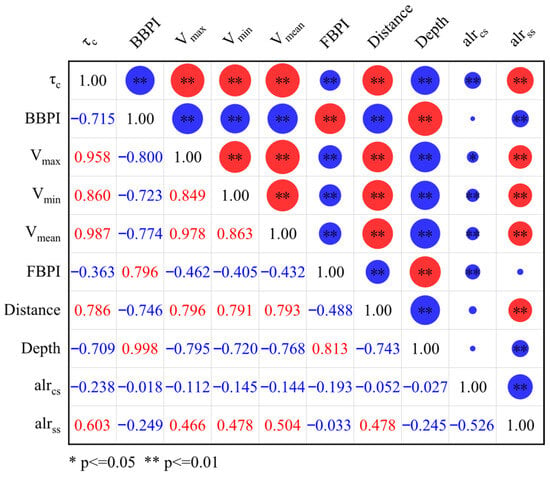
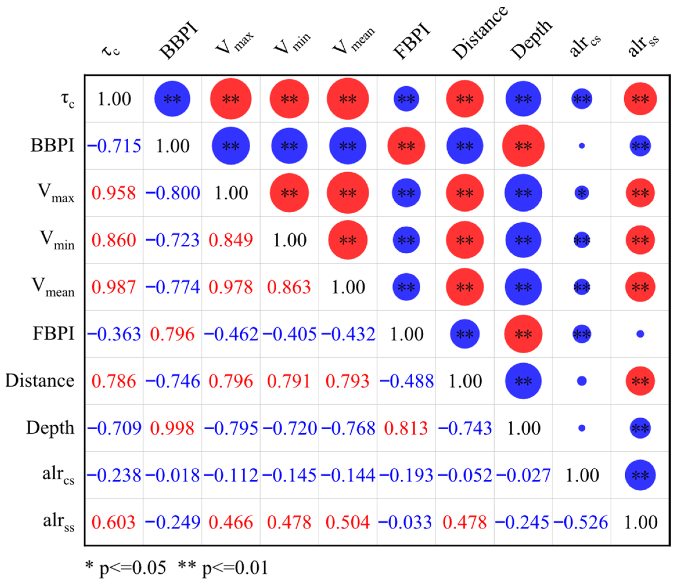
To assess monotonic relationships between environmental covariates and the sediment grain-size response variables, Spearman’s rank correlation coefficients (ρ) were calculated for alrcs and alrss against each predictor (Figure 5). Correlations between alrcs and the covariates are generally low in magnitude (|ρ| ≤ 0.238) and predominantly negative. The largest negative associations are observed with bed shear stress τc (ρ = −0.238, p < 0.01) and the fine-scale bathymetric position index FBPI (ρ = −0.193, p < 0.01). Relationships with other covariates are not significant, suggesting that variation in alrcs is likely influenced by multiple interacting factors, with limited explanatory power from any single environmental variable. In contrast, alrss shows clearer and more statistically robust correlations with several covariates. A positive correlation is found with τc (ρ = 0.603, p < 0.01). Positive correlations are also observed with hydrodynamic velocity variables (Vmax, Vmin, Vmean; ρ = 0.466–0.504, all p < 0.01) and with distance to the coastline (ρ = 0.478, p < 0.01). Negative correlations are present with the broad-scale bathymetric position index BBPI (ρ = −0.249, p < 0.01) and water depth (ρ = −0.245, p < 0.01). These results indicate that alrss is more sensitive to gradients in hydrodynamic energy and cross-shelf position than alrcs. Finally, alrcs and alrss are negatively correlated (ρ = −0.526, p < 0.01), which is consistent with the expected coupling of log-ratio variables under compositional constraints.
Figure 5.
Spearman correlation coefficients between alrcs/alrss and environmental covariates. Note: Statistical significance was evaluated at two levels. Red indicates a positive correlation, blue indicates a negative correlation, and the size of the circles represents the strength of the correlation.
3.2. Prediction of Sediment Grain-Size Fraction
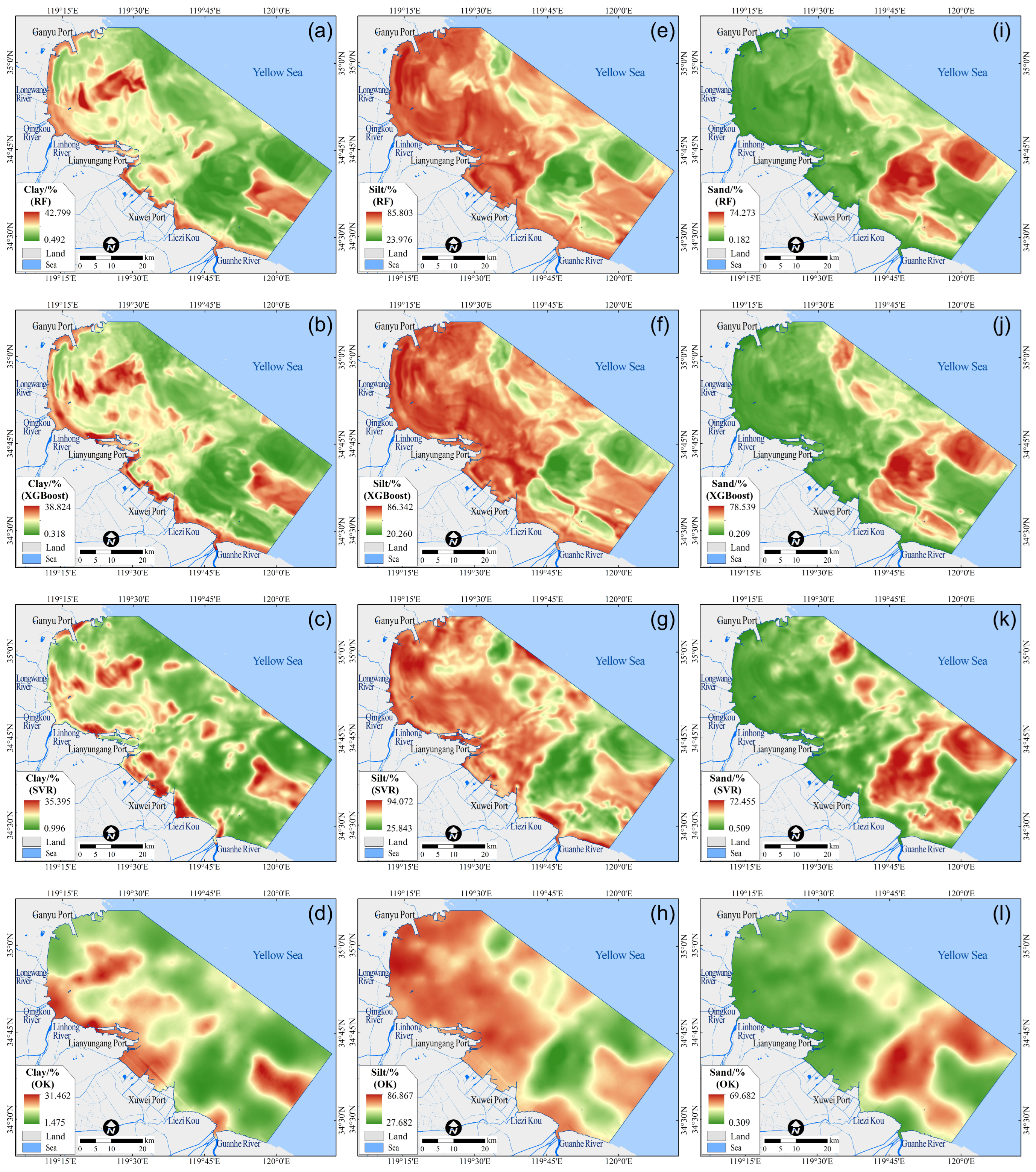
Using the alr-transformed variables (alrcs, alrss) and environmental covariates from sampling stations, RF, XGBoost, and SVR were trained to model nonlinear relationships. The trained models were then applied to the 60 m covariate rasters to predict alrcs and alrss, and an inverse transformation based on Equation (2) was used to obtain maps of clay (Figure 6a–c), silt (Figure 6e–g), and sand (Figure 6i–k). For comparison, ordinary kriging results are also presented for clay (Figure 6d), silt (Figure 6h), and sand (Figure 6l). The three machine learning methods show broadly consistent spatial patterns of sediment grain-size fractions. High clay values occur mainly in central Haizhou Bay and adjacent nearshore waters, silt is generally elevated in offshore waters north of Xuwei Port, and sand is concentrated on shallow shoals east of Liezikou, consistent with previous surveys of the offshore area of Lianyungang [20]. By comparison, OK reproduces the same broad distribution features—clay-enriched waters in central Haizhou Bay and adjacent nearshore zones, elevated silt north of Xuwei Port, and sand concentrated on the shoals east of Liezikou—but exhibits smoother gradients and more sample-controlled local extremes than the machine learning maps. The OK fields show more rounded patches and more diffuse boundaries, especially for the sand-rich shoal area (Figure 6l) and the patchy clay hotspots (Figure 6d).
Figure 6.
Predicted spatial distributions of sediment grain-size fractions generated by three machine learning models. Clay (%) predicted by (a) Random Forest (RF), (b) eXtreme Gradient Boosting (XGBoost), (c) Support Vector Regression (SVR), and (d) ordinary kriging (OK); silt (%) predicted by (e) RF, (f) XGBoost, (g) SVR, and (h) OK; and sand (%) predicted by (i) RF, (j) XGBoost, (k) SVR, and (l) OK.
Due to regularization and generalization constraints, predicted fraction ranges after inverse transformation are narrower than observed ranges: predicted minima exceed observed minima, and most predicted maxima fall below observed maxima. This reflects the models’ inherent tendency to dampen extremes for stability, which is evident for both ensemble methods (RF and XGBoost) and the kernel-based SVR. A similar smoothing effect is also observed in OK, where local peaks and troughs are more strongly attenuated. Among them, XGBoost yields the narrowest range shrinkage: predicted clay (0.318–38.824%), silt (20.260–86.342%), and sand (0.209–78.539%) closely align with observed distributions and indicate better fidelity to variability and overall predictive performance.
3.3. Mapping Results of Seabed Substrate Types
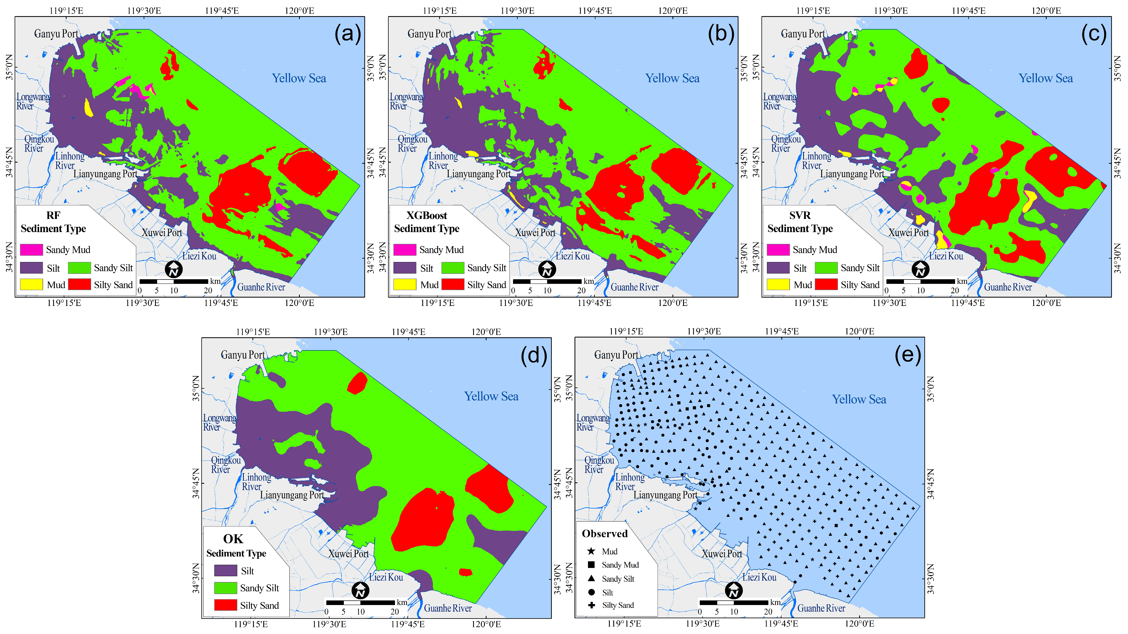
Based on predicted clay, silt, and sand rasters, substrate types were assigned to each grid cell per the Folk [38] ternary classification system, using ArcGIS raster algebra tools. Subsequently, substrate-type maps were generated for RF (Figure 7a), XGBoost (Figure 7b), and SVR (Figure 7c). For comparison, an OK-based substrate map was also produced (Figure 7d). The three machine learning maps show a consistent large-scale pattern. sZ and Z dominate central and eastern areas as broad, contiguous belts, whereas zS, M, and sM occur as scattered patches along belt margins. This pattern is consistent with the spatial structure indicated by the sampling stations (Figure 1). The OK map shows the same overall pattern with smoother boundaries and fewer small patches, and it does not identify the M and sM classes that appear in the machine learning maps.
Figure 7.
Seabed substrate types classified by the Folk scheme based on predicted grain-size fractions and observed sediment classes. (a) RF, (b) XGBoost, (c) SVR, (d) OK, (e) observed (427 sediment stations).
For dominant classes (sZ, Z), XGBoost best reproduces extent, boundary sharpness, and spatial juxtaposition, particularly in transition zones, where boundaries are distinct and misclassification is minimal. RF captures broad patterns but shows slight blurring and reduced boundary contrast between sZ and Z. SVR exhibits modest contraction of dominant zones and minor spatial displacement relative to observations.
For classes with limited samples (zS, M, sM), performance diverges more clearly. RF omits several zS patches, absorbing them into dominant substrates. XGBoost accurately locates most zS patches with good fidelity to size and shape; minor omissions of M and sM occur only in marginal areas with very low sample density. SVR places multiple M and sM patches, but their locations show poor agreement with observations and do not reproduce the true distribution patterns. In contrast, the OK map fails to resolve the two mud-related classes (M and sM), and most of these areas are absorbed into adjacent dominant substrates. OK also shows smoother boundaries and fewer small patches in transition zones, indicating weaker delineation of local heterogeneity than the machine learning maps.
Overall, XGBoost provides the most balanced substrate mapping, showing the highest agreement with observations and a more stable delineation of both the dominant belts and patches belonging to sparsely sampled classes. Most misclassifications are concentrated in transition zones between adjacent substrate types, whereas RF and SVR exhibit more pronounced misclassification. These differences are also evident in the Folk sediment classification ternary diagram, where RF and SVR deviate more substantially from the observed class distributions. Consequently, XGBoost provides robust cartographic support for characterizing the regional-scale spatial distribution of substrate types and for informing marine spatial planning and management.
3.4. Evaluation of Predictive Performance
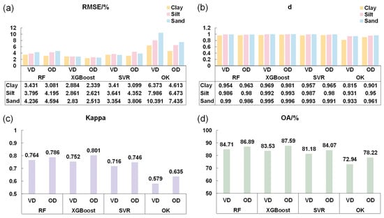
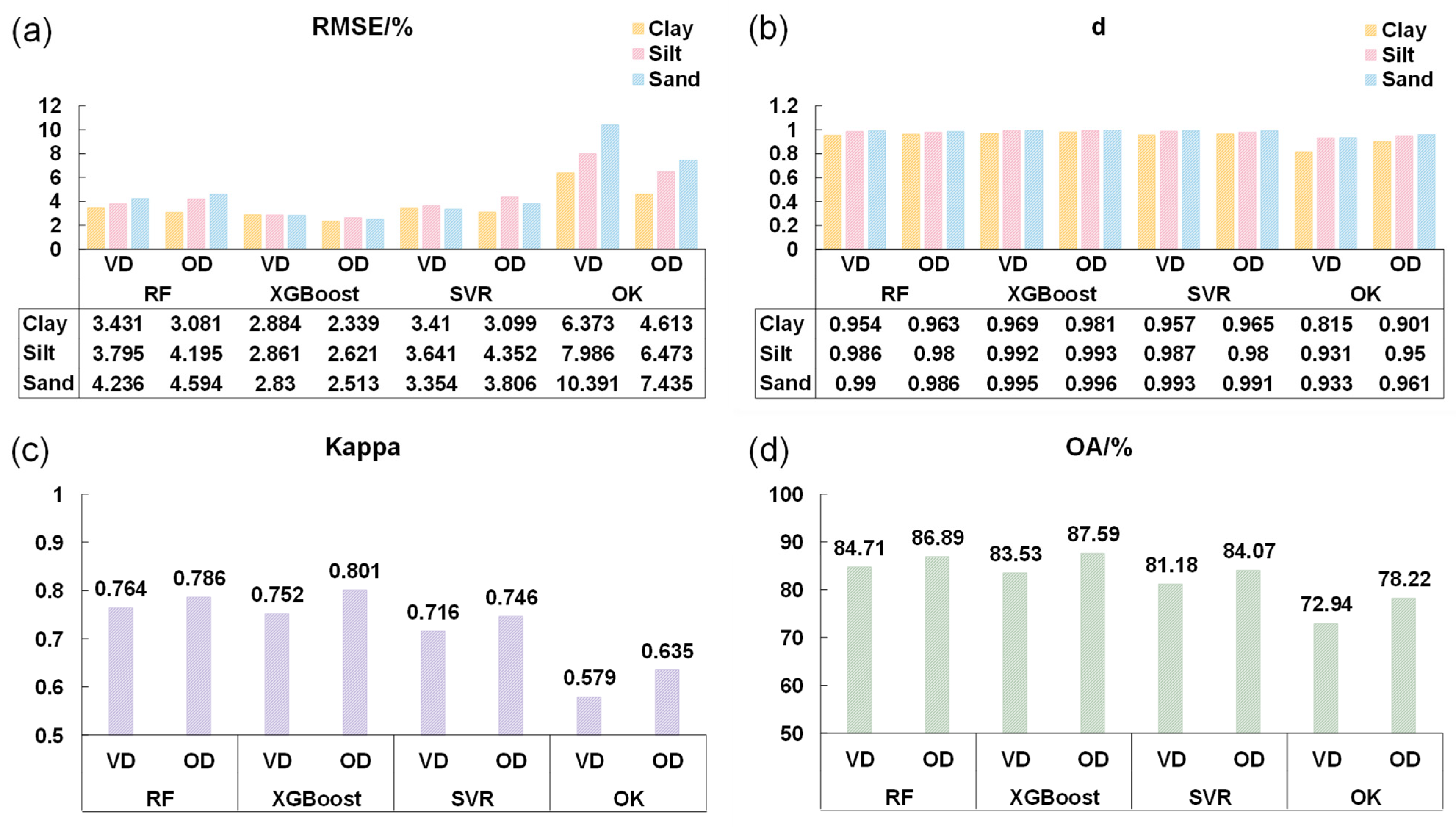
Predictive performance is quantified in Figure 8 and Figure 9, evaluating both continuous sediment grain-size fraction prediction (Figure 8a–d) and categorical substrate-type mapping (Figure 9a–d). It should be noted that the RMSE/d, OA/Kappa, and confusion matrix are the quantitative consistency indicators derived from the independent validation set, which was strictly reserved for final model evaluation and did not participate in the training process. For sediment grain-size fractions, XGBoost achieves the highest accuracy: on the validation dataset, its RMSE values for clay, silt, and sand are 2.884%, 2.861%, and 2.830%, respectively, which are lower than those of RF (3.431–4.236%), SVR (3.354–3.641%), and OK (6.373–10.391%). Corresponding Willmott’s d indices (0.969, 0.992, 0.995) further confirm superior model fidelity across all fractions. Metrics computed using the full dataset (Figure 8d) provide a reference that is consistent with the validation-based results.
Figure 8.
Accuracy assessment of sediment grain-size fraction prediction and seabed substrate-type mapping. (a) Root mean square error (RMSE, %) and (b) index of agreement for the predicted clay, silt, and sand fractions using RF, XGBoost, SVR, and OK. (c) Kappa and (d) overall accuracy (OA, %) for the corresponding Folk substrate-type maps derived from the predicted fractions. Metrics are reported for both the validation dataset and the overall dataset. Note: Vd = validation dataset; OD = overall dataset.
Figure 9.
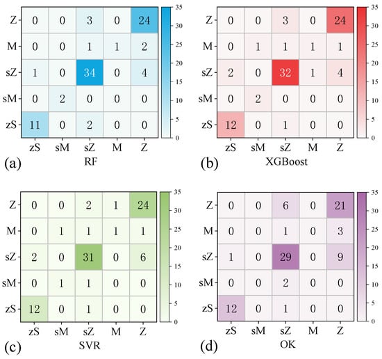
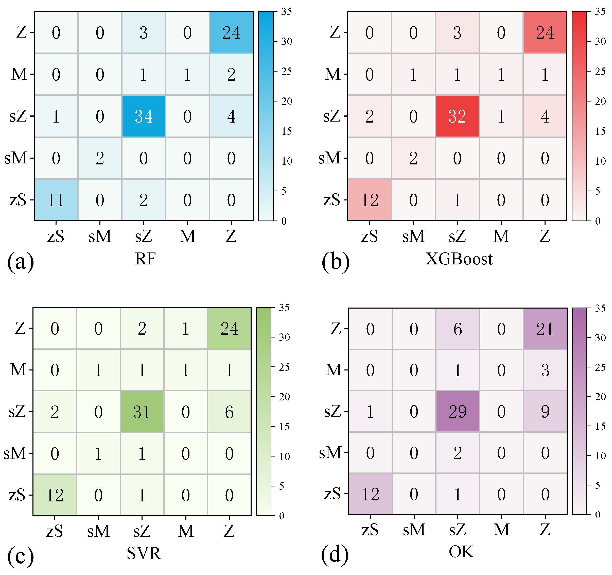
Confusion matrices for seabed substrate-type classification on the validation dataset. (a) RF, (b) XGBoost, (c) SVR, and (d) OK.
Across fractions, sand shows the highest RMSE, consistent with its largest coefficient of variation (CV = 0.83) and strongest spatial heterogeneity (Section 3.1). This reflects greater uncertainty in extrapolating from sparse point samples across highly variable shoal environments. In contrast, silt’s low CV (0.25) and spatial uniformity yield the lowest RMSE and highest d, confirming that prediction error scales directly with inherent sediment variability. Collectively, these statistical results align closely with the spatial patterns in Figure 6 and Figure 7, indicating that all models capture dominant gradients while XGBoost delivers the most statistically rigorous representation.
For substrate classification, overall accuracy (OA) and Cohen’s kappa on the validation dataset are RF (OA = 84.71%, kappa = 0.764), XGBoost (OA = 83.53%, kappa = 0.752), SVR (OA = 81.18%, kappa = 0.716), and OK (OA = 72.94%, kappa = 0.579). The three machine learning methods reach substantial agreement (kappa > 0.7), suggesting that the main substrate pattern is reproduced, whereas OK performs worse with a lower kappa (0.576) and OA (72.94%). The confusion matrices (Figure 9) show that most errors arise from two sources: confusion between the dominant classes Z and sZ in their transition area and unstable classification for classes with limited samples (zS, M, and sM). For the three machine learning methods, Z is classified consistently, with all 24 Z samples correctly identified by each model and only a few Z samples assigned to sZ (RF: 3; XGBoost: 3; SVR: 2). In contrast, sZ is more often assigned to Z (RF: 4; XGBoost: 4; SVR: 6), which matches the boundary patterns in Figure 7. OK exhibits the same error mode but more strongly, with a larger two-way mixing between Z and sZ. For classes with limited samples, the three machine learning methods correctly identify only one M sample, and the remaining M samples are mostly assigned to sZ or Z. The sM class is identified more reliably by RF and XGBoost (two correct samples each), whereas SVR correctly identifies only one and assigns the others mainly to sZ. In contrast, OK fails to identify mud and sandy mud altogether (no samples predicted as M or sM), and these samples are absorbed mainly into Z and sZ (Figure 9d). Overall, limited sample support, together with compositional similarity to dominant classes, makes marginal and patchy substrates harder to distinguish, and this limitation is most evident in OK for mud-related classes and in the transition zones between Z and sZ.
On the full dataset, XGBoost outperforms Random Forest in both aspects: it achieves higher accuracy for predicting the continuous grain-size fractions, as indicated by lower RMSE and higher d, and it also yields higher agreement in sediment-type identification, as reflected by OA and kappa. It should be emphasized that this study compares the predictive performance of three machine learning regression models. RMSE and d are direct metrics of regression fidelity for the predicted sand, silt, and clay fractions. In contrast, OA and kappa are indirect categorical metrics because they depend not only on the accuracy of the predicted fractions but also on the chosen sediment classification scheme. As a result, categorical agreement metrics can be less stable, particularly for samples near class boundaries where small numerical differences may change the assigned Folk class. Therefore, when OA and kappa differences among models are small, we place greater weight on the metrics that are directly tied to regression performance, namely RMSE and d, to determine the overall superiority of a model.
3.5. Assessment of Covariate Feature Importance
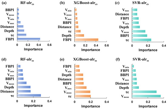
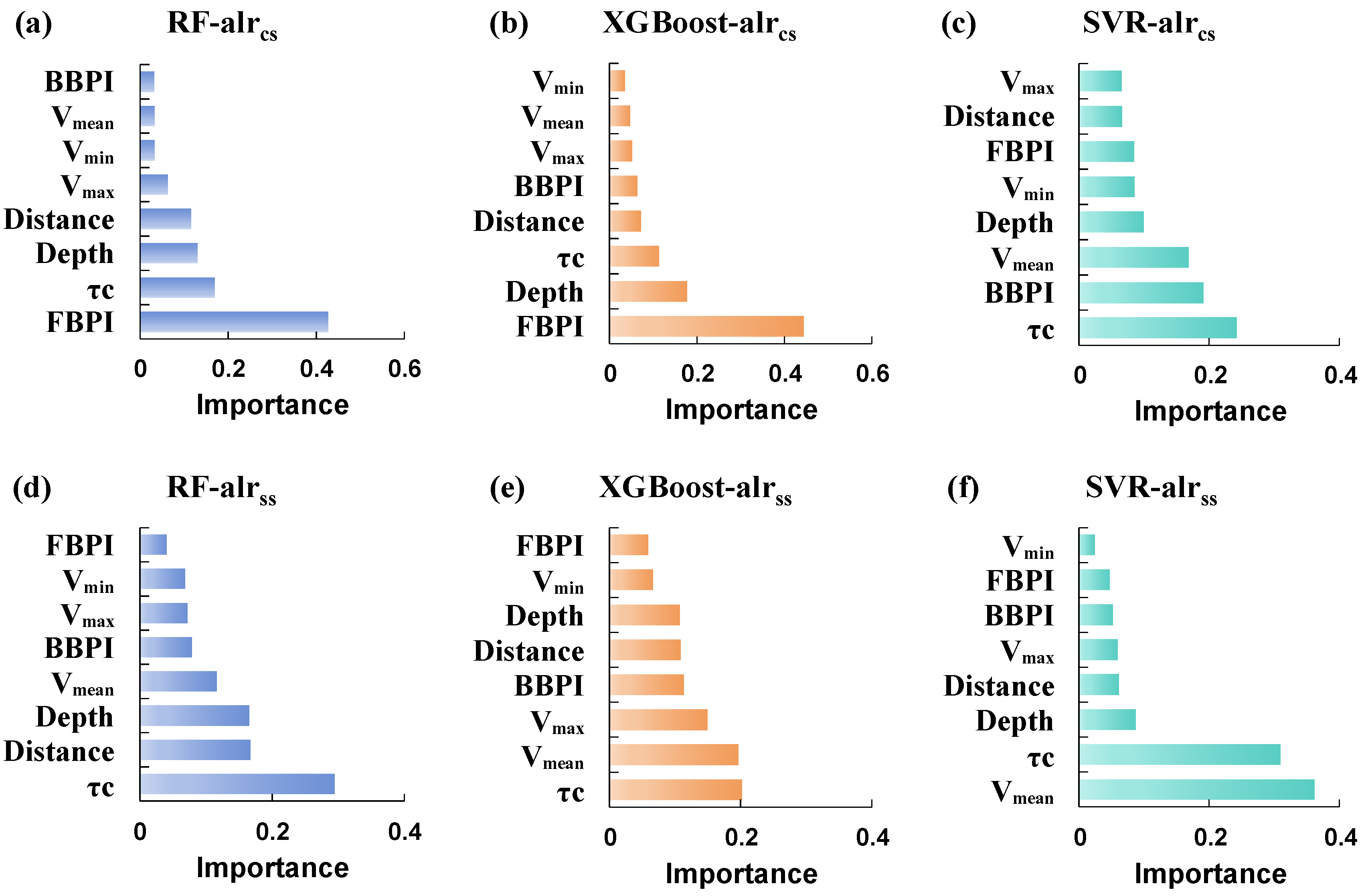
Figure 10 shows feature importance rankings for the two alr-transformed response variables, alrcs and alrss. For alrss, importance rankings are highly consistent across RF, XGBoost, and SVR: τc is consistently the top predictor (mean relative importance ≥ 42%), followed closely by Vmean and Vmax. This reflects alrss’s strong sensitivity to hydrodynamic intensity, consistent with its high Spearman correlation with τc (ρ = 0.603) and velocity metrics (ρ = 0.466–0.504). Because alrss is highly correlated with the sand fraction (ρ = 0.926, p < 0.01), the dominance of τc provides process-based support that hydrodynamic forcing is the primary control on the spatial distribution of sand in the study area. In particular, τc directly represents near-bed forcing that governs sediment entrainment, transport capacity, and grain-size sorting, whereas Vmean and Vmax further reinforce the role of flow intensity. Depth and Distance generally form a second tier, suggesting that sand distribution is driven mainly by hydrodynamic energy and the nearshore to offshore gradient, rather than by static bathymetry alone.
Figure 10.
Feature importance results for alrcs (a–c) and alrss (d–f) derived from (a,d) RF, (b,e) XGBoost, and (c,f) SVR.
In contrast, importance rankings for alrcs vary substantially across models. In RF and XGBoost, terrain-related covariates, especially FBPI and Depth, rank highest, whereas SVR assigns higher weights to τc and Vmean. This difference is expected given the complementary modeling mechanisms of tree-based and kernel-based methods. More importantly, alrcs represents the log ratio between clay and silt and is therefore closely linked to the clay fraction in the original compositional space (ρ = 0.927, p < 0.01). Consequently, the consistently high ranking of BPI-type terrain indices, particularly FBPI, supports the inference that the bathymetric position is a key factor shaping the spatial distribution of clay in the study area. This is consistent with a physical interpretation in which microtopography modulates clay accumulation through terrain-controlled depositional trapping in sheltered lows, combined with threshold-like resuspension under variable currents and spatially varying sediment supply along the land–sea gradient. Such coupled, nonlinear effects may be weak in simple pairwise correlations yet can be captured through model-based learning, and different algorithms may emphasize different aspects of these interactions. As a result, RF and XGBoost tend to produce sharper, terrain-aligned transitions, whereas SVR yields smoother patterns that are more strongly tied to continuous hydrodynamic gradients.
Taken together, the covariates can be grouped into three broad roles. First, τc acts as a robust universal driver, dominating alrss across all models and remaining among the top contributors for alrcs, highlighting bed shear stress as the primary dynamic control on grain-size differentiation. Second, terrain-mediated drivers, represented by FBPI and Depth, are emphasized by tree-based models and reflect geomorphic partitioning of depositional environments. Third, variables such as Vmin contribute little across models, likely due to information overlap with Vmean and Vmax and limited additional explanatory power at the regional scale.
Methodologically, XGBoost’s iterative residual fitting and L1/L2 regularization enable robust capture of both dominant continuous trends (e.g., offshore silt enrichment) and localized nonlinear interactions (e.g., FBPI-modulated clay accumulation in depressions) without overfitting sparse data. This balance explains its superior performance—highest fidelity in sediment grain-size fraction prediction (Section 3.4), clearest substrate boundaries (Section 3.3), and most stable rare-class identification—making it uniquely suited to nearshore systems where terrain and hydrodynamic coupling governs sediment patterning.
4. Discussion
This study evaluated three machine learning algorithms, RF, XGBoost, and SVR, for spatial prediction and mapping of nearshore seabed substrates. The aim was to produce accurate substrate maps that support the interpretation of depositional environments and inform marine resource development, utilization, and management. In the offshore area of Lianyungang, all three models reproduce the main regional pattern of substrate differentiation and generate substrate-type maps that are consistent with field observations. Differences among models are most apparent in transition zones and in the mapping stability of substrate types with limited samples. Integrated evaluation reveals that XGBoost achieves the most balanced overall performance. It preserves a realistic spatial structure while applying moderate regularization to extreme values and noticeably reducing class mixing in transitional areas, consistent with the inherent design principles of gradient boosting frameworks, particularly their capacity for nonlinear fitting and implicit regularization [33].
A substantial body of prior research has addressed method selection for seabed substrate mapping. Geostatistical interpolation techniques, especially kriging, have long been favored due to their rigorous quantification of spatial autocorrelation and theoretical grounding in regionalized variable theory [5,6]. Hybrid variants such as cokriging incorporate ancillary environmental covariates and are often used to leverage additional spatial information, with the aim of refining predictions and supporting uncertainty assessment. For instance, Jerosch et al. [39] demonstrated on the Beaufort Sea shelf that ordinary kriging adequately captured the spatial continuity of sediment grain size, whereas cokriging, incorporating terrain-derived predictors, yielded lower cross-validation prediction errors, suggesting potential gains in predictive consistency and spatial interpretability. Nevertheless, conventional geostatistical methods exhibit well-documented limitations: they tend to underperform when sample sizes are small or when rare substrate classes are present; moreover, their smoothing tendency often leads to the suppression or under-representation of minor substrate types by dominant ones, thereby obscuring fine-scale spatial heterogeneity. This pattern is reflected in the OK-derived map, which appears noticeably smoother and concentrates predictions in the dominant classes (zS, sZ, and Z), while the minority classes sM and M are not identified. In contrast, machine learning approaches can help address several of these constraints by learning flexible, nonlinear mappings between substrate classes and multivariate environmental covariates [40]. In this study, even SVR, which showed the weakest overall performance among the three models, achieved a 40% identification accuracy for the sparsely sampled sM substrate class, which is consistent with prior reports that machine learning models can be effective at representing minority or sparsely sampled classes in low-sample settings [41].
The fundamental divergence in predictive performance between geostatistical and machine learning paradigms stems largely from their contrasting assumptions and capacities regarding covariate integration. Geostatistical methods, particularly cokriging, incorporate auxiliary covariates through cross-variogram and covariance modeling, and their effectiveness depends on whether the target variable and the covariates exhibit a stable, modellable cross-covariance structure that can be adequately parameterized [42]. Machine learning models, by contrast, impose no a priori linearity assumptions. Their intrinsic architectures, such as recursive partitioning in RF [43], sequential residual correction in XGBoost [44], and implicit high-dimensional feature transformation via kernel functions in SVR [45], enable the effective capture of complex, nonlinear, and interactive relationships among predictors. In this study, for example, although marginal single-predictor linear signals are limited for alrcs, XGBoost successfully discriminates clay-rich from silt-rich deposits by jointly leveraging terrain and hydrodynamic variables. This finding aligns with Alharbi et al. [46], who highlighted the capacity of XGBoost to model nonlinear coupling effects among environmental drivers, which further underscore the superior flexibility and explanatory power of machine learning in covariate utilization.
Beyond predictive accuracy, machine learning methods offer a distinct advantage in mechanistic interpretation through quantitative assessment of variable importance. Geostatistical frameworks can incorporate only those covariates exhibiting statistically significant linear associations with the target variable; weakly correlated or inherently nonlinear predictors are either excluded or inadequately weighted, and no direct measure of relative contribution is available [47]. Machine learning models, however, provide principled, model-agnostic metrics, such as permutation importance or gain-based rankings, to objectively rank predictor influence [48]. In our analysis, all three algorithms consistently identify near-bed tidal current-induced shear stress (τc) and mean flow velocity (Vmean) as key driving factors for alrss substrate differentiation, which reinforces the established sedimentological principle that hydrodynamic sorting governs the spatial partitioning of sandy versus silty deposits [49]. Concurrently, the high importance assigned to terrain variables (e.g., bathymetric position index) for alrcs supports the conceptual model wherein topography indirectly modulates fine-grained sediment distribution by steering local hydrodynamic regimes—a mechanism previously proposed by Misiuk [50]. This quantitative attribution provides a process-based context for substrate maps, which is difficult to achieve using geostatistical methods alone.
The performance of any spatial prediction method is inherently influenced by data quality, sampling density, scale compatibility, and the complexity of the study area. Therefore, method selection should be based on empirical, context-specific validation rather than algorithmic preference alone, and multi-method comparison remains essential for identifying the most suitable approach for a given dataset and research objective [51]. In the present study, model performance was assessed using an independent hold-out set of in situ sediment samples, providing quantitative support for the predicted grain-size fractions and Folk-derived substrate classes under the available data conditions. Nevertheless, because no independent, spatially continuous ground-truth substrate map is currently available for the study area, true external map-to-map validation could not be performed, which should be recognized as an important limitation. In addition, uncertainties in the environmental covariates likely contribute to prediction error. For example, bathymetry derived from historical nautical charts may not fully resolve microtopographic features relevant to sediment distribution at the time of sampling [52].
These limitations also define the interpretative scope of the resulting maps. The current predictor set does not explicitly account for localized benthic structures, such as seagrass meadows, pipelines, or wrecks, and does not include high-resolution acoustic or geophysical datasets (e.g., multibeam bathymetry/backscatter, side-scan sonar, or sub-bottom profiles), which may reduce model robustness in areas where fine-scale seabed heterogeneity exerts strong control on sediment distribution. In addition, the primary objective of this study was to compare the performance of different models using the same input dataset and a consistent spatial resolution; therefore, a commonly used grid resolution of 60 m was adopted for all analyses. Nevertheless, spatial resolution may influence both model performance and the representation of substrate patterns [53], and the effects of scale should be investigated more explicitly in future work. The predicted maps should thus be interpreted primarily as regional-scale representations of nearshore surface sediment patterns, rather than as fine-scale characterizations of seabed heterogeneity or short-term depositional dynamics. This constraint is further compounded by the absence of dedicated sedimentation monitoring, which limits the direct assessment of ongoing sediment transport and deposition processes. Future research should therefore focus on integrating higher-resolution benthic and geophysical datasets, improving hydrodynamic representation, and developing multi-scale, process-oriented validation frameworks to enhance the robustness, interpretability, and transferability of nearshore substrate classification.
5. Conclusions
This study assessed the performance of RF, XGBoost, and SVR models for predicting nearshore sediment grain-size fractions (clay, silt, sand) and classifying Folk-derived substrate types in the Lianyungang offshore area, with OK used as a geostatistical benchmark. Overall, the three machine learning models achieved substantially improved predictive fidelity relative to OK, showing lower fraction prediction errors and higher substrate classification agreement, while OK produced a smoother map dominated by the major classes and failed to delineate the two mud-related minority classes (sM and M).
All three machine learning models reproduced the regional pattern of finer sediments nearshore and coarser sediments offshore, but they differed in three critical domains: (1) retention of extreme values and fine-scale variability in continuous predictions; (2) boundary sharpness in transition zones (e.g., between Z and sZ); and (3) stability in identifying rare classes (zS, M, sM). XGBoost exhibited the most balanced performance, retaining sediment grain-size variability, minimizing transitional mixing, and capturing small patches with high fidelity. RF excelled in noise-robust gradual transition delineation, while SVR showed fragmented boundaries and less stable patch locations. These results highlight that substrate mapping’s core challenge lies in resolving transitional boundaries and marginal patches, a distinction masked by aggregate accuracy metrics.
Feature importance analysis revealed a mechanistic hierarchy: τc and current velocity dominated sand spatial distribution, while terrain indices (FBPI, Depth) drove clay distribution pattern in tree-based models (validating microtopographic modulation of flow confinement and fine-sediment trapping). Beyond accuracy improvements, machine learning transforms substrate maps into process-informed tools by linking spatial patterns to sediment transport physics, enabling mechanistic interpretation of depositional environments and providing actionable inputs for marine spatial planning and coastal engineering. The high-resolution datasets generated are directly applicable to coastal geomorphology research and infrastructure siting.
Author Contributions
Conceptualization, J.Y. and F.L.; Data curation, J.Y., L.G. and X.L.; Formal analysis, J.Y. and F.L.; Methodology, J.Y., S.J. and X.L.; Validation, J.Y. and L.G.; Visualization, J.Y., L.G. and S.J.; Writing—original draft, J.Y., F.L. and L.G.; Writing—review and editing, J.Y., F.L. and L.G.; Supervision, F.L. All authors have read and agreed to the published version of the manuscript.
Funding
This study was partly supported by the National Natural Science Foundation of China (NSFC, No. 41976187).
Data Availability Statement
The data presented in this study are available on request from the corresponding author.
Conflicts of Interest
The authors declare no conflicts of interest.
References
- Halpern, B.S.; Walbridge, S.; Selkoe, K.A.; Kappel, C.V.; Micheli, F.; d’Agrosa, C.; Bruno, J.F.; Casey, K.S.; Ebert, C.; Fox, H.E. A global map of human impact on marine ecosystems. Science 2008, 319, 948–952. [Google Scholar] [CrossRef] [Scilit] [PubMed]
- Guan, Y.; Qu, Y.; Zhang, N.; Xiao, Y.; Rong, B.; Zhang, P. Evaluating the land-sea coordination in Chinese coastal cities from an integrated and water eco-environmental perspective. Stoch. Environ. Res. Risk Assess. 2025, 39, 1501–1516. [Google Scholar]
- McArthur, M.; Brooke, B.; Przeslawski, R.; Ryan, D.; Lucieer, V.; Nichol, S.; McCallum, A.; Mellin, C.; Cresswell, I.; Radke, L.C. On the use of abiotic surrogates to describe marine benthic biodiversity. Estuar. Coast. Shelf Sci. 2010, 88, 21–32. [Google Scholar]
- Beaman, R.J.; Daniell, J.J.; Harris, P.T. Geology–benthos relationships on a temperate rocky bank, eastern Bass Strait, Australia. Mar. Freshw. Res. 2005, 56, 943–958. [Google Scholar] [CrossRef] [Scilit]
- Jerosch, K. Geostatistical mapping and spatial variability of surficial sediment types on the Beaufort Shelf based on grain size data. J. Mar. Syst. 2013, 127, 5–13. [Google Scholar] [CrossRef] [Scilit]
- Lark, R.; Marchant, B.; Dove, D.; Green, S.; Stewart, H.; Diesing, M. Combining observations with acoustic swath bathymetry and backscatter to map seabed sediment texture classes: The empirical best linear unbiased predictor. Sediment. Geol. 2015, 328, 17–32. [Google Scholar] [CrossRef] [Scilit]
- Li, J.; Heap, A.D. A Review of Spatial Interpolation Methods Forenvironmental Scientists; Record 2008/23; Geoscience Australia: Canberra, ACT, Australia, 2008.
- Verfaillie, E.; Du Four, I.; Van Meirvenne, M.; Van Lancker, V. Geostatistical modeling of sedimentological parameters using multi-scale terrain variables: Application along the Belgian Part of the North Sea. Int. J. Geogr. Inf. Sci. 2009, 23, 135–150. [Google Scholar] [CrossRef] [Scilit]
- Stephens, D.; Diesing, M. Towards quantitative spatial models of seabed sediment composition. PLoS ONE 2015, 10, e0142502. [Google Scholar] [CrossRef] [Scilit]
- Wilson, B.R.; Brown, C.J.; Sameoto, J.A.; Lacharité, M.; Redden, A.M.; Gazzola, V. Mapping seafloor habitats in the Bay of Fundy to assess megafaunal assemblages associated with Modiolus modiolus beds. Estuar. Coast. Shelf Sci. 2021, 252, 107294. [Google Scholar] [CrossRef] [Scilit]
- Li, M.Z.; Hannah, C.G.; Perrie, W.A.; Tang, C.C.; Prescott, R.H.; Greenberg, D.A. Modelling seabed shear stress, sediment mobility, and sediment transport in the Bay of Fundy. Can. J. Earth Sci. 2015, 52, 757–775. [Google Scholar] [CrossRef] [Scilit]
- Li, J.; Tran, M.; Siwabessy, J. Selecting optimal random forest predictive models: A case study on predicting the spatial distribution of seabed hardness. PLoS ONE 2016, 11, e0149089. [Google Scholar] [CrossRef] [Scilit] [PubMed]
- Wang, C.; Jiang, X.; Liu, H.; Li, Y. Prediction of the shear wave speed of seafloor sediments using an XGBoost model based on physical and grain size parameters. Front. Mar. Sci. 2024, 11, 1307768. [Google Scholar] [CrossRef] [Scilit]
- Wang, J.; Hou, Z.; Chen, Y.; Li, G.; Kan, G.; Xiao, P.; Li, Z.; Mo, D.; Huang, J. The Acoustic Attenuation Prediction for Seafloor Sediment Based on in-situ Data and Machine Learning Methods. J. Ocean Univ. China 2025, 24, 95–102. [Google Scholar] [CrossRef] [Scilit]
- Wadoux, A.M.-C.; Minasny, B.; McBratney, A.B. Machine learning for digital soil mapping: Applications, challenges and suggested solutions. Earth-Sci. Rev. 2020, 210, 103359. [Google Scholar] [CrossRef] [Scilit]
- Houghton, J.; Nichols, T.; Griffiths, J.; Simon, N.; Utley, J.; Duller, R.; Worden, R. Automated Classification of Estuarine Sub-Depositional Environment Using Sediment Texture. J. Geophys. Res. Earth Surf. 2023, 128, e2022JF006891. [Google Scholar] [CrossRef] [Scilit]
- Nemani, S.; Cote, D.; Misiuk, B.; Edinger, E.; Mackin-McLaughlin, J.; Templeton, A.; Shaw, J.; Robert, K. A multi-scale feature selection approach for predicting benthic assemblages. Estuar. Coast. Shelf Sci. 2022, 277, 108053. [Google Scholar] [CrossRef] [Scilit]
- Wang, F.; Yu, J.; Liu, Z.; Kong, M.; Wu, Y. Study on offshore seabed sediment classification based on particle size parameters using XGBoost algorithm. Comput. Geosci. 2021, 149, 104713. [Google Scholar] [CrossRef] [Scilit]
- Huang, Z.; Siwabessy, J.; Cheng, H.; Nichol, S. Using multibeam backscatter data to investigate sediment-acoustic relationships. J. Geophys. Res. Ocean. 2018, 123, 4649–4665. [Google Scholar] [CrossRef] [Scilit]
- China Bay Geographic Exploration Committee. China Bay Gazetteer, Vol. 4: Bays of the Southern Shandong Peninsula and Jiangsu Province; Ocean Press: Beijing, China, 1993. [Google Scholar]
- Yu, J.; Cao, X.; Chen, Z.; Wen, W.; Zhang, C.; Liu, Y. Analysis of tidal and tidal current characteristics in the offshore waters of Lianyungang during the winter of 2019. Mar. Sci. Bull. 2020, 53–60. [Google Scholar]
- Callesen, I.; Keck, H.; Andersen, T.J. Particle size distribution in soils and marine sediments by laser diffraction using Malvern Mastersizer 2000—Method uncertainty including the effect of hydrogen peroxide pretreatment. J. Soils Sediments 2018, 18, 2500–2510. [Google Scholar] [CrossRef] [Scilit]
- Wentworth, C.K. A scale of grade and class terms for clastic sediments. J. Geol. 1922, 30, 377–392. [Google Scholar] [CrossRef] [Scilit]
- Aitchison, J. The statistical analysis of compositional data. J. R. Stat. Soc. Ser. B (Methodol.) 1982, 44, 139–160. [Google Scholar] [CrossRef] [Scilit]
- Egozcue, J.J.; Pawlowsky-Glahn, V.; Mateu-Figueras, G.; Barcelo-Vidal, C. Isometric logratio transformations for compositional data analysis. Math. Geol. 2003, 35, 279–300. [Google Scholar] [CrossRef] [Scilit]
- Blanchy, G.; Saneiyan, S.; Boyd, J.; McLachlan, P.; Binley, A. ResIPy, an intuitive open source software for complex geoelectrical inversion/modeling. Comput. Geosci. 2020, 137, 104423. [Google Scholar] [CrossRef] [Scilit]
- Martín-Fernández, J.A.; Barceló-Vidal, C.; Pawlowsky-Glahn, V. Dealing with zeros and missing values in compositional data sets using nonparametric imputation. Math. Geol. 2003, 35, 253–278. [Google Scholar]
- Wright, D.; Pendleton, M.; Boulware, J.; Walbridge, S.; Gerlt, B.; Eslinger, D.; Sampson, D.; Huntley, E. ArcGis Benthic Terrain Modeler (BTM), version 3.0; Environmental Systems Research Institute: Redlands, CA, USA; National Oceanic and Atmospheric Administration Coastal Services Center, Massachusetts Office of Coastal Zone Management: Boston, MA, USA, 2012. Available online: http://esriurl.com/5754 (accessed on 23 December 2024).
- CNES. FES2022 (Finite Element Solution) Tidal Model; CNES: Paris, France, 2024. [CrossRef]
- Lund-Hansen, L.C.; Valeur, J.; Pejrup, M.; Jensen, A. Sediment fluxes, re-suspension and accumulation rates at two wind-exposed coastal sites and in a sheltered bay. Estuar. Coast. Shelf Sci. 1997, 44, 521–531. [Google Scholar] [CrossRef] [Scilit]
- Breiman, L. Random forests. Mach. Learn. 2001, 45, 5–32. [Google Scholar]
- Pedregosa, F.; Varoquaux, G.; Gramfort, A.; Michel, V.; Thirion, B.; Grisel, O.; Blondel, M.; Prettenhofer, P.; Weiss, R.; Dubourg, V. Scikit-learn: Machine learning in Python. J. Mach. Learn. Res. 2011, 12, 2825–2830. [Google Scholar]
- Chen, T. XGBoost: A Scalable Tree Boosting System; Cornell University: Ithaca, NY, USA, 2016. [Google Scholar]
- Cortes, C.; Vapnik, V. Support-vector networks. Mach. Learn. 1995, 20, 273–297. [Google Scholar] [CrossRef] [Scilit]
- Willmott, C.J. On the validation of models. Phys. Geogr. 1981, 2, 184–194. [Google Scholar] [CrossRef] [Scilit]
- Foody, G.M. Status of land cover classification accuracy assessment. Remote Sens. Environ. 2002, 80, 185–201. [Google Scholar] [CrossRef] [Scilit]
- Sabharwal, C. Cohen’s Kappa statistic and newKappaStatistic for measuring and interpreting inter-rater agreement. Int. J. Res. Eng. Sci. 2021, 9, 23–28. [Google Scholar]
- Folk, R.L. The distinction between grain size and mineral composition in sedimentary-rock nomenclature. J. Geol. 1954, 62, 344–359. [Google Scholar] [CrossRef] [Scilit]
- Diesing, M.; Green, S.L.; Stephens, D.; Lark, R.M.; Stewart, H.A.; Dove, D. Mapping seabed sediments: Comparison of manual, geostatistical, object-based image analysis and machine learning approaches. Cont. Shelf Res. 2014, 84, 107–119. [Google Scholar] [CrossRef] [Scilit]
- Farooq, I.; Bangroo, S.A.; Bashir, O.; Shah, T.I.; Malik, A.A.; Iqbal, A.M.; Mahdi, S.S.; Wani, O.A.; Nazir, N.; Biswas, A. Comparison of random forest and kriging models for soil organic carbon mapping in the Himalayan Region of Kashmir. Land 2022, 11, 2180. [Google Scholar] [CrossRef] [Scilit]
- Wang, Y.; Yuan, F.; Cammarano, D.; Liu, X.; Tian, Y.; Zhu, Y.; Cao, W.; Cao, Q. Integrating machine learning with spatial analysis for enhanced soil interpolation: Balancing accuracy and visualization. Smart Agric. Technol. 2025, 11, 101032. [Google Scholar] [CrossRef] [Scilit]
- Yalçin, E. Cokriging and its effect on the estimation precision. J. South. Afr. Inst. Min. Metall. 2005, 105, 223–228. [Google Scholar]
- Lee, C.; Park, S.; Yoon, D.; Yi, B.-Y.; Lim, M. Enhancing seabed sediment classification with multibeam echo-sounding and self-training: A case study from the East Sea of South Korea. Front. Earth Sci. 2025, 13, 1550244. [Google Scholar]
- Yun, J.; Park, J.; Choo, H.; Lee, H.-M.; Won, J. Data-driven machine learning models for predicting engineering properties in deep-sea sediments. Sci. Rep. 2025, 15, 44987. [Google Scholar] [PubMed]
- Lee, A.-S.; Enters, D.; Huang, J.-J.S.; Liou, S.Y.H.; Zolitschka, B. An automatic sediment-facies classification approach using machine learning and feature engineering. Commun. Earth Environ. 2022, 3, 294. [Google Scholar] [CrossRef] [Scilit]
- Alharbi, H.S. Interpretable and Calibrated XGBoost Framework for Risk-Informed Probabilistic Prediction of Slope Stability. Sustainability 2025, 17, 10122. [Google Scholar] [CrossRef] [Scilit]
- Verfaillie, E.; Van Lancker, V.; Van Meirvenne, M. Multivariate geostatistics for the predictive modelling of the surficial sand distribution in shelf seas. Cont. Shelf Res. 2006, 26, 2454–2468. [Google Scholar] [CrossRef] [Scilit]
- Greenberg, M.; Frid, V. Physics-guided random forest classification of marine sediments using frequency-dependent acoustic reflection spectra. Appl. Sci. 2025, 15, 12930. [Google Scholar] [CrossRef] [Scilit]
- Chen, J.; Zhang, J.; Liu, S.; Chen, W.; Qin, Y.; Wu, S. Grain size distribution pattern of surface sediments and its implications for transportation trend: A case from the waters off Zhongsha Islands, the South China Sea. Mar. Geol. Quat. Geol. 2021, 42, 15–27. [Google Scholar]
- Misiuk, B.; Lecours, V.; Bell, T. A multiscale approach to mapping seabed sediments. PLoS ONE 2018, 13, e0193647. [Google Scholar] [CrossRef] [Scilit]
- Keskin, H.; Grunwald, S. Regression kriging as a workhorse in the digital soil mapper’s toolbox. Geoderma 2018, 326, 22–41. [Google Scholar] [CrossRef] [Scilit]
- An, N.N.; Hong, P.V.; Binh, N.A.; Thao, G.T.P.; Van Tinh, L.; Hanh, N.C.; Tran, T.T. Spatiotemporal dynamics of suspended sediment in coastal Mekong Delta: A hydrodynamic modelling approach under tropical monsoon climate. Sci. Rep. 2025, 15, 5851. [Google Scholar] [CrossRef] [Scilit]
- Guo, Z.; Adhikari, K.; Chellasamy, M.; Greve, M.B.; Owens, P.R.; Greve, M.H. Selection of terrain attributes and its scale dependency on soil organic carbon prediction. Geoderma 2019, 340, 303–312. [Google Scholar] [CrossRef] [Scilit]

Disclaimer/Publisher’s Note: The statements, opinions and data contained in all publications are solely those of the individual author(s) and contributor(s) and not of MDPI and/or the editor(s). MDPI and/or the editor(s) disclaim responsibility for any injury to people or property resulting from any ideas, methods, instructions or products referred to in the content. |
© 2026 by the authors. Licensee MDPI, Basel, Switzerland. This article is an open access article distributed under the terms and conditions of the Creative Commons Attribution (CC BY) license.