From Detection to Inspection: A Virtual Reference Framework for Automated Road Marking Degradation Assessment

Abstract

Ensuring the visibility of road markings is critical for traffic safety, yet current inspection methods remain either prohibitively expensive (retroreflectivity) or subjective (manual assessment). This article introduces the Random Generated Reference (RGR) method, a novel automated solution for quantifying marking degradation using a standard on-board camera. The proposed pipeline is a complete protocol from video acquisition to road marking inspection and validation of the inspection that combines deep learning with computer vision: YOLOv8 is employed for robust detection, while a unique algorithm generates a “perfect virtual reference” that dynamically replicates the real scene’s geometry and illumination conditions, including shadows. By computing pixel-level deviations between the observed marking and this ideal reference, the system assigns a continuous degradation score aligned with the UK CS126 standard. Experimental validation was conducted on a real-world circuit yielding over 20,000 detections. Verification via Cochran sampling demonstrates that 68% of the automated assessments fall within one class of human inspection. This proof-of-concept confirms the viability of an approach based on generating the ground truth and scene conditions—such as illumination, shadows, rain, traffic, etc.—for road marking inspection.

1. Introduction

Road markings are a fundamental element of road infrastructure. They are applied as paint on the pavement—most often white, or yellow—and are usually embedded with glass microbeads to enhance retroreflectivity and thus improve nighttime visibility [1]. They serve several essential functions: guiding drivers along the roadway, delineating lanes and right-of-way, and providing ongoing feedback on vehicle position under both ordinary and challenging conditions, such as nighttime driving or rainfall. Doing so, they contribute significantly to reducing the risk of accidents [2]. However, road markings are not permanent; both the paint and the glass microbeads undergo progressive deterioration due to mechanical wear from traffic and environmental influences. This deterioration diminishes visibility and retroreflective performance, eventually making markings harder to read or even invisible, which undermines their safety role. From a road-safety perspective, it is important to implement regular inspection and maintenance programs that monitor the condition of markings over time and restore their visibility before safety is compromised.

The phenomenon of retroreflection is the reference measurement to evaluate marking degradation and to model marking durability [3,4,5]. However, this operation requires costly equipment such as ECODYN3, which severely limits inspection frequency. Since the 1990s [6], alternative approaches have been proposed, notably manual inspections, conventional image-processing methods applied to on-board camera footage, and deep learning approaches that use on-board cameras. Conventional image-processing methods have been widely used for the detection [7,8,9,10] and inspection [11] of road markings. While they perform well in ideal conditions, their effectiveness typically degrades when scene illumination, weather, traffic, geometry or time of day vary. Deep learning techniques are currently the preferred approach for marking detection [12]; unlike classical methods, they learn to recognize markings under heterogeneous conditions from large datasets, thereby improving extraction and classification. Deep learning-based methods typically employ cameras [12,13] to acquire and analyze road data.

Inspection methods based on deep learning generally aim to qualify or quantify degradation by training on ground truth annotations. The majority of studies only propose a single score without trying to connect it to some agreed standards of measurement [14,15,16] such as retroreflection or contrast. When this verification is done, it seems that there is no correlation [17].

Based on this observation, we believe it is necessary to produce a dedicated framework for estimating the degradation of road markings using camera-based inspection. To avoid starting with an almost complete lack of knowledge on this subject, and to directly propose a framework acceptable to road authorities, we suggest drawing inspiration from the standards governing visual inspection of markings and attempting to update them for the practice of filming roads and processing images with AI.

We distinguish two topics: filming the road according to a precise geometry and assessing the degradation of the markings. For the first point, the EN 1436 [18] standard already proposes a visibility geometry for markings, which forms the basis for the operation of dynamic retroreflectometers such as ECODYN and therefore for marking inspection.

However, for the second topic, few standards exist today such as the UK CS126 [19], or the SS 589:2013 [20]. We believe that connecting an estimated degradation score—regardless of the method—to an existing standard visual assessment is a necessary step to validate this score. In this study, we propose a protocol from video acquisition to marking inspection and validation of the inspection, using a deep learning approach that aims to detect road marking using an on-board camera and deduce a degradation score partially inspired by the UK CS126 standard. Five steps are discussed:

• Select a deep learning-based road marking detector using on-board camera data. In this study, a YOLOv8 [21] model was trained using the Mapillary dataset [22].
• Derive a degradation score partially inspired by the CS-126 standard for the detected markings. Our proposed method, termed Random Generated Reference (RGR), operates in three stages:
  • Generate an idealized numerical representation of the detected road marking, modeling the acquisition conditions (e.g., shadows) and the geometric characteristics of the marking. Conceptually, this approach allows inspection under arbitrary conditions—whether optimal or adverse.
  • Compare, at the pixel level, the detected marking with its generated ideal counterpart to quantify differences.
  • Deduce a quantitative degradation score adapted to the CS126 standard.
• Validate detection results under operational conditions using a classification performance metric.
• Validate the RGR score under operational conditions by comparing it with manual inspection results obtained by assessors in accordance with the CS-126 standard.
• Assess the interaction between the detection stage and the inspection stage.

Our proposed solution is grounded in a literature analysis. Section 2 presents the related work. Section 3 describes our choice of road marking detector. Section 4 outlines the inspection method. Section 5 explains the Cochran sampling technique used. Section 6 presents our experiments and the results obtained. Section 7 discusses the method used in this paper. Section 8 concludes the work.

2. Related Work

Our literature review is split into three subjects: road marking detection, attributing a degradation score and current standards for road marking visual assessments.

2.1. Road Marking Detection Methods

Road marking detection has been a well-studied area since 2010. With the development of autonomous vehicles, accurate lane detection and road-context understanding are critical for the development of ADAS and fully automated driving systems. Deep learning approaches currently dominate the literature [7,12,23], which is attributable to the ability of convolutional neural networks (CNNs) to automatically learn hierarchical features from data, removing the need for hand-crafted parameters and providing superior generalization across diverse and challenging environmental conditions in which traditional methods often fail. The review conducted by Zhang et al. [12] serves as our primary reference in road marking detection because this study hierarchizes a hundred road marking detection solutions. As a road construction and maintenance company, we are focused on the raw detection of road markings only. It is a necessary first step to deduce road marking damage degree.

Some examples of deep learning strategies using a camera have been proposed: modified CNN architectures such as SCNN from X. Pan et al. [24], specifically designed to capture spatial relationships of lane markings; generative adversarial networks (GANs) such as EL-GAN from M. Ghafoorian et al. [25] and Ripple-GAN from Zhang et al. [26]; attention mechanisms [27,28,29]; or even detectors specialized for damaged markings [30].

Our priority is to select a performant detection method rather than to favor any particular algorithm. In this respect, Zhang et al. [12] rank the available approaches according to the performance metrics reported by their authors. From that review we adopt an indicative minimum F1-score of 75% as an acceptable baseline: detection is therefore imperfect but sufficient for inspection purposes. This interpretation must be qualified by four methodological limitations highlighted in the review. First, there is no consensual evaluation metric, although the F1-score is widely used. Second, reported metrics are computed on the authors’ test datasets. No consensual test dataset exists to compare the performance of different models. Third, these metrics are not estimated under operational field conditions. Fourth, there is currently no consensus on either the visibility geometry or a reference standard defining what constitutes a degraded road marking.

Given these limitations, model selection should be guided by reported theoretical performance but complemented by an independent verification protocol in operational conditions; the visibility geometry should be tied to the standard commonly used in road marking inspections; and a reference definition of what constitutes a (visual) degraded road marking must be adopted, using a standard visual assessment such as CS126. Only methods that can be validated in such operational settings are considered acceptable as our clients will demand a verification of the AI results.

From that perspective, an object-detection model such as YOLOv8 [21,31,32,33] is sufficient. This solution has proven itself in a previous study [34]. YOLOv8 builds on the strengths of earlier single-stage detectors while introducing key architectural changes to improve flexibility: it replaces the standard C3 backbone blocks with the C2f module to promote richer feature representation and improved gradient flow, and it abandons anchor-based prediction in favor of an anchor-free, decoupled head. By separating classification and localization, the model better accommodates the irregular shapes and aspect ratios of road markings without relying on manually tuned anchor boxes, thereby simplifying training for complex geometries. Following the literature and recent studies, YOLO models seem widely used and reliable to detect and estimate the damage degree of road marking.

Regarding visibility geometry, the most widely used standard in the road inspection industry is EN-1436 [18], which defines the angle and distance at which a road object should be visible to the driver. Our detection method will follow this standard.

Alternatively, deep learning approaches have also been applied to LiDAR data. The main purpose of applying LiDAR to road inspection is to reconstruct the road environment in 3D. However, it is possible to train deep learning models to identify which 3D points correspond to road markings. For instance, C. Wen et al. [35] proposed a modified U-net for marking extraction, CNNs for classification, and conditional GANs to reconstruct missing markings. Furthermore, Z. Dong et al. [36] introduced Marking-DNet, an enhanced DeepLabV3+ architecture integrating CBAM and OCR attention mechanisms to segment 2D laser pavement images. With LiDAR data, it is not only possible to detect road markings but also to estimate their retroreflection, making LiDAR a valuable road inspection sensor [37,38,39,40,41]. These studies all stress the importance of establishing proper visibility geometry, since this parameter is far more sensitive for LiDAR than for camera-based solutions. However, our main focus is the camera, as it is easy to deploy and cost-effective.

2.2. Inspection and Attributing Road Marking Damage Degree

A new generation of solutions proposed not only to detect markings but also to classify or to quantify their degradation. In this section, we distinguish two families of damage-degree evaluation: qualification methods, which assign a categorical quality score (i.e., a class indicating the marking’s condition); and quantification methods, which aim to produce a precise scalar measure of the degree of damage. Table 1 summarizes the presented methods with their advantages, limitations, and performance.

Table 1. Recent studies in road marking damage degradation inspection.

	Study	Method	Advantages	Limitation	Performance
Qualification These methods aim to qualify the road marking damage.	Chen et al. (2024) [42]	Object detection (CFG_SI_YOLO), CoordConv, Focal-EIoU and SimAM attention	The method achieves real-time speed, handles blurred details and addresses sample imbalance.	The defect dataset is limited to five specific defects, and the model needs further optimization.	F1-score: 85.7%
					mAP: 82.8%
	Wu et al. (2024) [43]	Semantic segmentation, IPM and thresholding for assessment to construct a dataset for YOLOv11	The authors created a public dataset (RMDDD). The method achieves real-time speed.	Images are manually cropped, introducing a risk of human error. While improved, data imbalance persists in the dataset.	mAP: 73.5%
	Manongga & Chen (2025) [44]	Detection with YOLOv9, VAE reconstruction, fuzzy logic classification	Ambiguous and imprecise conditions are handled with fuzzy logic. The use of unsupervised learning works with limited damage sample.	Detection of severe damaged marking (>80% of damage) fails.	Classification accuracy: 72.95%
Quantification These methods aim to precisely quantify the road marking damage.	Kong et al. (2022) [14]	DeepLab V3 and segmentation, IPM and adaptative local thresholding	Robust method for lighting with adaptative threshold.	Sensitive to shadows, rain, or surface water.	Accuracy: 98.04%
					mIoU: 82.70%
	Wang et al. (J. Imaging) (2025) [15]	Two-stage semantic segmentation (intact region vs. residual pixels), ALFVC and BFE modules	Presents a high segmentation and boundary retrieval performances in a lightweight and performant approach.	Method is limited for severe localized damage.	mIoU: 89.44%
					Minimum damage rate error: 0.22%
	Wang et al. (Automation) (2025) [16]	Oriented object detection (improved YOLOv8) and minimum rectangle bounding box math modeling	Can handle perspective distortion and is effective for severe marking damage.	It is less efficient, and errors are possible for complex geometry (like curved lines). It is sensitive to lighting conditions.	mAP: 97.4%
					Minimum damage degree error: 0.54%

Concerning the qualification methods, Chen et al. [42] designed the CFG_SI_YOLO model, based on the advantages of the YOLO model. It utilizes multi-channel coordinate convolution (CoordConv) to enhance spatial awareness and capture fine target details. It incorporates a Focal-EIoU loss function to address sample imbalance and a Similarity Attention Module (SimAM) to mitigate interference from similar objects. Wu et al. [43] created a system that uses semantic segmentation and inverse perspective mapping (IPM) to calculate a numerical damage ratio by comparing undamaged parts to the total marking region. This data is then used to create a dataset to train a YOLOv11 detector that directly classifies markings into three severity grades based on the calculated ratios. Manongga and Chen [44] employed a hybrid approach using YOLOv9 to detect road markings and a Variational Autoencoder (VAE) that attempts to reconstruct images and calculate anomaly scores on this reconstruction. The scores are then processed by a fuzzy logic system to classify the damage into three qualitative levels: normal, slight, or serious damage.

Concerning the quantification methods, Kong et al. [14] uses a method that utilizes DeepLab V3+ for semantic segmentation and IPM to analyze street-view imagery at a city scale. It quantifies damage by applying adaptive local thresholding to extract the actual paint area, which is then compared against the theoretical recovered shape of the marking. Wang et al. (Journal of Imaging) [15] designed a framework that employs a two-stage semantic segmentation process that separately identifies residual pixels and the total original marking region. It integrates an Asymmetric Large Field-of-View Contextual (ALFVC) module and a Boundary Feature Enhancement (BFE) module to ensure precise shape reconstruction for damage quantification. Wang et al. (automation) [16] created a method to establish a mathematical model between road markings and their minimum bounding rectangles (MBRs) using an improved oriented object detection algorithm based on YOLOv8. It estimates the theoretical intact area from the detected rectangle and compares it to the actual pixels to quantify the damage degree.

The main limitation of the cited studies is that their degradation scores are not compared or linked to established visual assessment standards such as UK CS126 [19] or Singapore SS 589:2013 [21]. As a result, those scores cannot be directly used to justify maintenance interventions for clients. In this paper, we propose a quantified degradation score and investigate its correlation with the CS126 visual assessment standard.

2.3. CS126 Standard and Alternatives

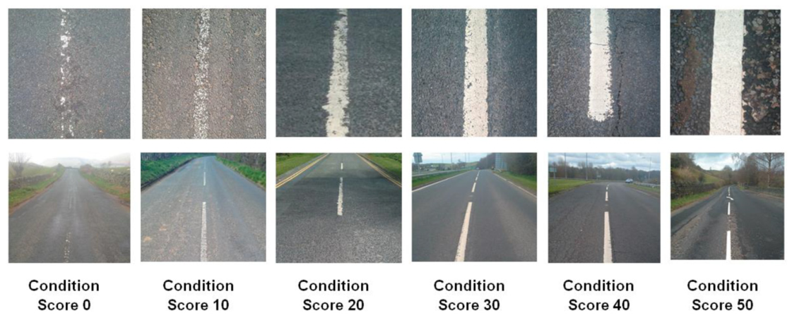
The CS126 standard is our reference standard for road marking visual assessment as it is European, and proposes a quantitative score and relatively simple and precise scale for damage road markings. Figure 1 and Table 2 summarize the official definition of the wear score. It classifies markings into six discrete categories (0, 10, 20, 30, 40, and 50) where 0 corresponds to a non-existent or residue-only marking and 50 to a no obvious wear marking.

Figure 1. Visual assessment scoring for wear (official definition, CS126 [19] Appendix C).

Table 2. Visual assessment scoring for wear (official definition, CS126 [19] Table B.1).

Assessment	Wear Index/Score	Defect Type When Score Is Averaged
Non-existent, residue only	0	Critical defect
Barely visible	10	Critical defect
Visible, but has randomly spaced small bare spots	20	Potentially critical defect—judgment required taking into account location and function. Plan should be put in place to manage.
Marginal—some visible wear, large bare spots	30	Non-critical defect
Very little wear	40	Non-critical defect
No obvious wear	50	No defect

According to the standard [19]—Appendix B: “The visual assessment system should be applied to each road marking and aggregated over 100m. The assessment should not mix materials or line types i.e. each line type should be associated with its own average score. In the case of lane dividing lines, each lane line should also be associated with its own average score”. In this paper, we simplify the study at the image scale, and not the 100 m scale. It will be the subject of a future paper.

Unfortunately, the CS126 standard applies only to line markings and provides just six example images, as shown in Figure 1. Known alternatives include standard SS 589:2013 or local requirements such as the Dutch one based on the European standard EN 1436 [18], described in CROW Publication 380 in 2018 [45]; however, the first is not a European standard, which means it is not considered in France, even though it is also based on wear-damage assessment, and the second one offers only qualitative grading (A+, A, B, C, and D). No equivalent standard is known for other types of road markings.

In this paper, our main objective is to attribute a rating to every road scene we capture. The adapted aggregation method over the 100 m required by the standard must be the subject of a future study but is out of scope for now as we try first to validate our method.

3. Road Marking Detection per YOLOV8

We distinguish two main tasks: the detection of road markings, and their inspection. Concerning the detection, the YOLOv8 model is trained on the Mapillary dataset [22,46]. Mapillary is a large road scene description dataset across all continents, referencing lots of different roads. Their images are in great and varying resolution and ideal for training object-detection models such as YOLOv8. In our case:

• Classes “marking--continuous—dashed” and “marking--continuous—solid” are merged into one class called “Line”.
• Classes “marking--discrete--arrow--left”, “marking--discrete--arrow--right”, “marking--discrete--arrow--split-left-or-straight”, “marking--discrete--arrow--split-right-or-straight”, and “marking--discrete--arrow--straight” are merged into one class called “Arrow”.
• Class “marking--discrete--crosswalk-zebra” is renamed “Crosswalk”.
• Other classes such as “marking--discrete--symbol—bicycle” are considered but not studied here for simplicity.

Upon processing an input road image, YOLOv8 outputs a detection log consisting of the region of interest (ROI) bounding each detected marking, the marking’s predicted class, and a segmentation mask delineating the exact pixel region of the marking. ROIs are expressed as bounding boxes (bbox). They are defined by four values, referred to as XYXY. The first two values represent the two-dimensional coordinates of the upper-left corner of the box, while the last two correspond to the coordinates of the lower-right corner. By using these coordinates in conjunction with the original road scene image, it is possible to extract all regions of interest (ROIs) containing road markings. This process effectively isolates the markings from the rest of the image data. These extracted results are the foundation of the proposed inspection method. Error in this stage will propagate to the inspection one.

4. Proposed Method: The Random Generated Reference

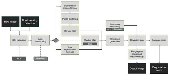
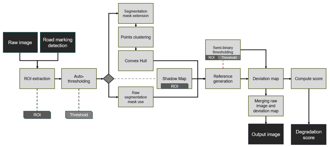
The Random Generated Reference (RGR) method enables the quantitative analysis of road marking deterioration using a single on-board camera. It is designed to accommodate a wide range of environmental conditions—such as low visibility, shadows and contrast variations—in order to assign a deterioration score to the markings under examination. RGR is the procedural, random generation of a virtual reference marking that replicates the visual conditions of the real scene. This perfect-condition virtual marking serves as a baseline under the same imaging conditions as the actual marking. By computing the difference in appearance between the real marking and its virtual counterpart, a difference map is produced. This map is then used to derive a quantitative deterioration score for the marking. The processing pipeline is illustrated in Figure 2 and will be illustrated with a sample crosswalk detected by YOLOv8 and shown in Figure 3.

Figure 2. The pipeline of the method. Black squares represent input and output elements. A gray square represents a step of the pipeline. The ROI and threshold are two intra-output elements used later in the pipeline.

Figure 3. ROI of a crosswalk detected by our YOLOv8.

4.1. Auto-Thresholding

The auto-thresholding algorithm determines a threshold value that separates the road marking from the road surface. The output is a binary mask, where the marking appears in white and the road in black. This process is intended to remove irrelevant areas (the road) at the pixel level, isolating the areas of interest (the markings). This preliminary step enables the reconstruction of markings despite their deterioration later in the inspection pipeline.

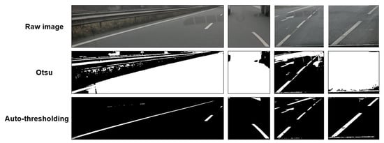
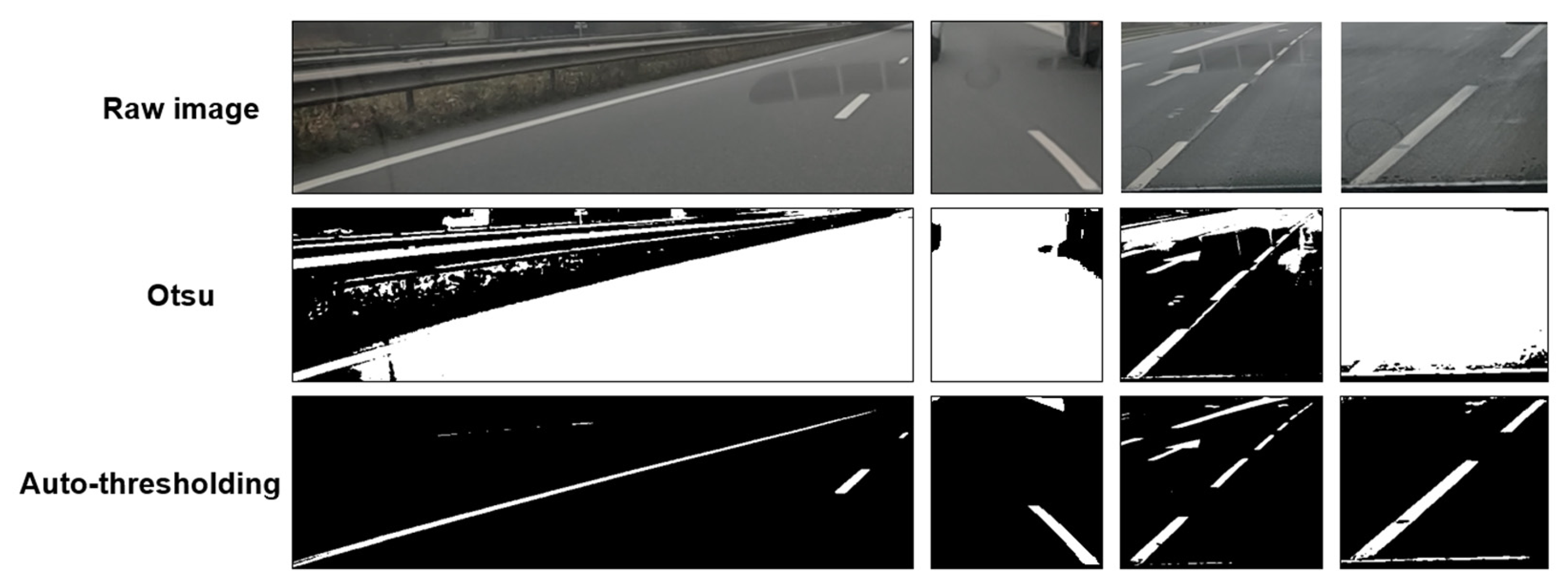
Although Otsu’s binary thresholding algorithm [47] is generally effective, the auto-thresholding algorithm developed here is more suited for our needs (Figure 4). It relies on the assumption that an image containing road markings typically consists of a gray to black region (the road) and a lighter, white region (the markings). Pixel value frequencies are shown on a distribution diagram.

Figure 4. Binary ROIs of detected road markings: a comparison between Otsu’s technique and ours.

In our case, this diagram should exhibit a prominent distribution peak corresponding to gray values and a smaller one corresponding to white values. The goal is to identify the correct local minimum between these gray and white peaks. Certain cases arise where the white peak is larger than the gray, or where the distribution of one or both is minimal.

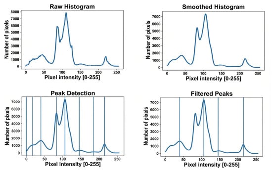
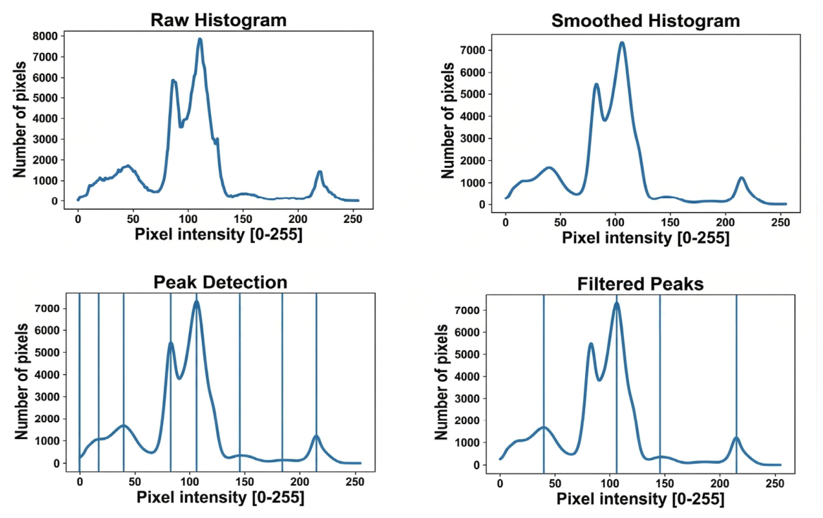
The auto-thresholding algorithm is designed to handle these scenarios. Figure 5 illustrates the preprocessing chain performed by the auto-thresholding procedure. First, the image histogram is computed. Then, the histogram curve is smoothed to eliminate irregular peaks, thereby preserving essential information while reducing noise. From the smoothed curve, the algorithm locates peaks, which are then filtered to retain only significant ones. This filtering operates as follows: a peak is discarded if its distribution value falls below a user-defined percentage of the histogram’s maximum distribution value, or if it is too close to a larger nearby peak. Our user defined percentage is 5% (0.05) and the value of the filter radius to check nearby peaks is 35.

Figure 5. Auto-thresholding pre-processing visualization.

At this stage, the main process begins. First, the largest peak in the histogram is arbitrarily designated as representing the distribution of gray values. If this peak is neither isolated nor the last in the list, it implies that the white value peak lies to its right and is the last peak. In this case, the threshold is defined as the local minimum between the largest peak and this last peak, corresponding to the smallest distribution value in that interval. If the largest peak is either the only peak or the last peak in the histogram, this indicates one of two scenarios: either the white value distribution is too low for a distinct peak to appear, or the white distribution is so dominant that the largest peak—initially attributed to gray values—corresponds to the white values. Under these conditions, the threshold is determined by iteratively shifting to the right (toward higher intensity or white values) from the first value below a user-defined percentage of the peak’s height.

Once the threshold is established, the average pixel value of the image is calculated. If this average falls below a very low threshold, indicating that the image is predominantly black, it suggests that the largest peak represents the distribution of white values. In this case, the algorithm is applied in reverse: if the peak is neither isolated nor the first peak, the threshold is set as the local minimum between this peak and the preceding one. If the peak is isolated or the first in the list, the cursor shifts iteratively to the left until an appropriate threshold value is found. Finally, if no peaks are detected, the algorithm starts from the maximum histogram value and treats this as the sole peak, applying the procedure described above. Figure 6 shows the auto-thresholding’s output, for the sample crosswalk.

Figure 6. Example of auto-thresholding’s output for the sample crosswalk.

4.2. Segmentation Mask Extension

The segmentation mask is obtained from the YOLOv8 detection logs and provides a spatial indication, with varying degrees of accuracy, of the location of the road marking. Due to inconsistencies in this accuracy, auto-thresholding refined the detected region. Following auto-thresholding, the processing pipeline diverges into two distinct paths: one dedicated to convex shapes and another to concave shapes. Convex markings are directed to an alternative pipeline regrouping an extension process applied to the segmentation mask, a point clustering process and a convex hull reconstruction method, whereas concave markings bypass this alternative pipeline and proceed directly to the reference generation phase, as a convex hull reconstruction method is not suited for concave shapes. At this stage, the segmentation mask is simply retrieved and prepared for the subsequent processing step.

For convex shapes, the extension of the segmentation mask constitutes a preparatory operation for the reconstruction of the markings. Since the mask provided by the detection process is not sufficiently reliable, the extension is applied to ensure complete coverage of the marking elements. This enlargement defines a restricted processing area beyond which no computation is carried out. By combining the extended segmentation mask with the auto-thresholded image, it becomes possible to isolate and process only the road markings, effectively suppressing any spurious data introduced by auto-thresholding.

4.3. Point Clustering

Point clustering identifies clusters corresponding to the constituent elements of the same road marking when they are separated by the roadway. Such elements may include the individual stripes of a crosswalk or the separate dashes of a broken line. Since YOLOv8 segmentation produces a mask that encompasses the entire marking rather than its separate parts, clustering is required to distinguish these components. A Canny edge detector is applied to the auto-thresholded image. Every white pixel is treated as a point. The goal is to group these points into local clusters. To avoid the O(N²) complexity of pairwise distance comparisons, we organize the point cloud using an optimized spatial structure. We employ a k-dimensional tree (k-d tree), which recursively partitions the plane into hierarchical zones along the X and Y axes. This organization enables zone search, automatically discarding zones that lie beyond a specified proximity to an anchor point. A search radius is then defined, beyond which two points are not considered neighbors. Clustering is performed by iterative propagation according to the following procedure:

• The first point in the list not yet assigned to any cluster becomes the anchor. A whole new cluster is assigned to this anchor.
• Query the k-d tree to return all neighbors within a sphere centered on the anchor and with its radius equal to the predefined search distance.
• Assign the returned points to the anchor’s cluster and push them in a processing stack.
• While the stack is not empty, pop the first point, becoming the new anchor. This anchor is already associated with the current cluster.
• Repeat steps 2 and 3 for this new anchor: search for unassigned neighbors, assign the anchor’s cluster to them and push them in the processing stack.
• When the stack is empty, return to step 1 to locate the next point without a cluster. This point becomes the anchor of a new cluster, and the propagation process repeats.

This approach ensures that all elements of a marking, even those separated by road gaps, are effectively grouped into distinct clusters for further analysis. Figure 7 shows the point clustering output, for the sample crosswalk.

Figure 7. Example of point clustering output for the sample crosswalk. Each color represents a different cluster of points.

4.4. Convex Hull

Once each point has been assigned to a cluster, a convex hull can be computed for each cluster. The convex hull of a point cloud is defined as the minimal convex polygon that encloses all points in the set, its edges passing through the outermost points. This geometric envelope is employed to reconstruct regions of the marking that are degraded or partially missing. From each convex hull, a corresponding convex mask can be extracted, serving to fill in the missing sections of the marking. The difference between this convex mask and the auto-thresholding result can then be computed. The combination of these two elements provides the prototype with essential information: the precise threshold delineating the road surface from the marking, and an estimated reconstruction of the complete marking area. This reconstructed representation is subsequently used to generate the reference shape for further processing. Figure 8 shows the convex hull method output, for the sample crosswalk.

Figure 8. An example of convex hull method output for the sample crosswalk. The top image represents the computed convex hull. The bottom image represents the extracted convex mask from the computed convex hull.

4.5. Shadow Map

The shadow map attempts to generate an image representing the brightness areas of the image in a simplified manner. This is a prototype method that still needs to be improved. The first step is to convert the image into perceived lightness defined by the ISO/CIE 11664-4 standard [48], i.e., an image that attempts to represent the human eye’s perception of brightness as accurately as possible. To do this, the image’s Red–Green–Blue (RGB) space must first be linearized, as it is gamma-corrected to more accurately encode the image data according to the human eye’s perception. Equation (1) follows the IEC [49] 61966-2-1 (sRGB) specification [50], which is built upon the CIE [51] 1931 standard observer [52] and D65 illuminant [53]. C_linear represents the three red, green and blue channels linearized. C_sRGB represents the initial gamma-corrected RGB channels.

$$C_{linear}=\left\{\begin{array}{cc}\hfill {\displaystyle \frac{C_{sRGB}}{12.92}},& C_{sRGB}\le 0.04045\hfill \\ \hfill {\left({\displaystyle \frac{C_{sRGB}+0.055}{1.055}}\right)}^{2.4},& C_{sRGB}>0.04045\hfill \end{array}\right.$$

(1)

Once the RGB space has been linearized, the luminance must be calculated. The ITU-R BT.709 standard [54] proposes the following formula (Equation (2)). Finally, the perceived lightness $L^{\ast }$ is estimated (Equation (3)) [48].

$$Y=R_{linear}\ast 0.2126+G_{linear}\ast 0.7152+B_{linear}\ast 0.0722$$

(2)

$$L^{\ast }=\left\{\begin{array}{cc}\hfill Y\ast 903.3,& Y\le 0.008856\hfill \\ \hfill Y^{{\displaystyle \frac{1}{3}}}\ast 116,& Y>0.008856\hfill \end{array}\right.$$

(3)

The second step of the process involves labeling the brightness levels within the image. The number of labels is defined by the user in the method parameters. Each label is assigned a central value, determined according to the selected number of labels and the distribution of pixel intensity values in the image. Once these central values are established, each pixel is assigned to the label whose central intensity value is closest to its own. This procedure reduces the continuous range of brightness values to a discrete set, thereby delineating regions of similar illumination across the image. The third step consists of smoothing these regions to mitigate image noise. A median filter is applied region by region, ensuring localized noise suppression without blurring region boundaries excessively. After each region has been individually smoothed, a global median filter is applied to the entire image to complete the noise reduction process. This operation yields a label mask that is subsequently applied to the perceived light image. The final step is the computation of the shadow map. By overlaying the label mask onto the perceived light image, the average perceived brightness value is calculated for each labeled region. This average value (named avg) is then attributed to its respective area. Furthermore, for each region a shadow weight (named S_w) is computed according to the empirically derived Equation (4).

$$S_w=\left\{\begin{array}{cc}\hfill \left|1-\left({\displaystyle \frac{1}{\min \left(avg\ast 0.0135; 1\right)}}\right)\right|,& avg<25\hfill \\ \hfill \left|1-\left({\displaystyle \frac{1}{\min \left(avg\ast 0.018; 1\right)}}\right)\right|,& avg\ge 25\hfill \end{array}\right.$$

(4)

Coefficients 0.0135 and 0.018 were determined through a series of trial-and-error experiments. The ceiling is reached when the average value (avg) is 55 or higher; in that case we considered shadow weighting unnecessary for the subsequent steps of the method (meaning S_w = 0). Conversely, we found that when avg is below 25—meaning the area is fairly dark—the 0.018 coefficient proved slightly too weak for the weighting. A second series of trials and errors led us to adopt 0.0135 to achieve a more appropriate shadow weighting. If the average value equals zero, Equation (4) is skipped as a safety measure, and the shadow weight is set to zero. However, this situation should never occur in real conditions, since the camera never captures a completely dark environment. Figure 9 shows the shadow map result for the sample crosswalk.

Figure 9. Generated shadow map for the sample crosswalk.

4.6. Reference Generation

The current generation module implements a four-step procedure, described as follows:

• For each pixel of the reference image (whose spatial dimensions are determined from the input image), a grayscale intensity value is sampled within the user-defined interval bounded by a lower and an upper limit. For this prototype, we defined value 210 as the lower limit and 250 as the upper limit.
• A first Gaussian blur is applied to the reference image to spatially diffuse intensity values and produce an interleaving of darker and lighter regions. The kernel size of this Gaussian blur is (3, 3).
• The blurred image is sharpened, which enhances local contrast and yields a crisper image while promoting the formation of more coherent, less randomly distributed intensity clusters. The formula used to sharpen the blurred image is $I_r\ast 1.5-I_b\ast 0.5$. $I_r$ is the random image obtained in step 1, and $I_b$ is the blurred image obtained in step 2. From step 1 to step 3, this technique is called Unsharp Mask.
• A second Gaussian blur is applied to mildly spread the intensity clusters, producing a texture that better approximates the appearance of a pristine photographed road marking. The kernel size of this Gaussian blur is (3, 3).

This reference is applied within a rectangle with the dimensions of the recovered ROI. Once this version has been generated, there are two additional steps. The first one is to blend in the shadows calculated from the shadow map. The second step consists of cutting out the reference to reproduce the detected marking. The convex mask previously computed is used. By blending the two, we obtain our generated reference. Figure 10 shows the random generated reference for the sample crosswalk.

Figure 10. The random generated reference for the sample crosswalk.

4.7. Semi-Binary Thresholding

At the same time, the actual marking must be extracted to enable comparison with the reference generated earlier. We employ the threshold determined previously during the auto-thresholding stage to perform a semi-binary thresholding operation: all pixel values below the threshold (i.e., corresponding to the road surface) are set to black, while values above the threshold (i.e., corresponding to the marking) are left unchanged. The result is an image in which the marking is delineated from its background. Figure 11 shows the semi-binary thresholding output for the sample crosswalk.

Figure 11. Semi-binary thresholding output for the sample crosswalk.

4.8. Deviation Map

The deviation map encodes per-pixel discrepancies between the generated reference and the extracted actual marking. These deviations are normalized and converted into a similarity score: higher scores indicate greater resemblance to the reference, while lower scores indicate larger deviations. The result is stored as an image encoded in the conical HSV color space. Unlike the RGB space, HSV represents color by an angle (H, hue), a radial distance from the cone axis (S, saturation) and a height (V, value). Hue = 0° corresponds to red, hue = 120° to green, with intermediate angles passing through orange, yellow and light green. This representation supports both a compact numerical encoding of differences and an intuitive visual rendering. For each pixel of an 8-bit unsigned image the applied formula is Equation (6), using Equation (5) as the raw difference value between the reference and the real marking. Parameters i and j are the 2D pixel coordinates. R is the reference. M is the real road marking. S_w is the shadow weight.

$${\delta }_{i,j}=\max \left({\displaystyle \frac{R_{i,j}-M_{i,j}}{255}};0\right)$$

(5)

$${\Delta }_{i,j}=\max \left(1-{\delta }_{i,j}{e}^{{\delta }_{i,j}\ast S_w}; 0\right)$$

(6)

Empirically, we propose to use exponential weighting together with the previously computed shadow weight to adapt the deviation measure to real road illumination. Illumination is spatially non-uniform; darker zones may be misinterpreted as degradation if raw differences are used. For instance, a pixel of value 200 that falls into shadow might drop to 100, producing a raw difference of 100, whereas a very dark pixel of value 5 that becomes 0 only loses 5 points. Because the reference models an ideal marking under typical road illumination, raw differences penalize losses in bright regions much more strongly. By introducing an adaptive term that depends on the original intensity (the shadow weight) and applying an exponential mapping, the metric becomes less prone to false positives in shaded areas and remains sensitive to meaningful degradations in bright zones. Figure 12 shows the computed deviation map.

Figure 12. The deviation map computed for the sample crosswalk. The colors used are a spectrum between green, yellow and red. Green represents areas of the road marking where there is no degradation. Red represents areas of the road marking where the degree of damage is at the maximum. Everything between (such as light green, yellow, and orange) represents the degree of damage of the road marking.

4.9. The Proposed RGR Score

$$Score=Med\left({\left\{{\Delta }_{i,j}\right\}}_{i=0\dots n, j=0\dots n}\right)\ast 50$$

(7)

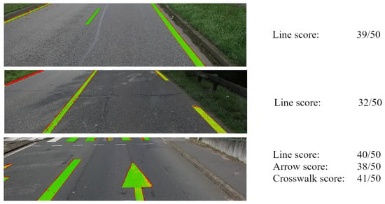
The final score for the analyzed markings is defined by Equation (7). The initial score ranges from 0 to 1 and is subsequently multiplied by 50 to express it on the same scale as the CS126 visual assessment standard. Each marking has an individual score, enabling the tracking of the exact score for every detected road marking. In this study, however, only the scene-level scores are considered. These scores are expressed as a single value per marking class; all lines detected in a given image contribute an individual score for each instance yet yield a single general score for the entire class. This general score is computed in the same manner as the single marking score; however, instead of computing the median across all pixels of a single marking, the median is computed across all points belonging to the same road marking class. This approach avoids averaging the scores of individual markings, which are themselves derived from a median. Figure 13 shows the score computed for three randomly chosen scenes. The third scene provides a clear illustration of the method’s capabilities and limitations. It includes: a line that is correctly detected and inspected; a line missed by YOLOv8 (on the left); two arrows detected and inspected, the second being only partially present in the scene; and a crosswalk detected and inspected, although one band has been missed. This scene thus summarizes the strengths and current shortcomings of our implementation.

Figure 13. Examples of the scores computed on three different road scenes. The colors used are a spectrum between green, yellow and red. Green represents areas of the road marking where there is no degradation. Red represents areas of the road marking where the degree of damage is at the maximum. Everything between (such as light green, yellow, and orange) represents the degree of damage of the road marking.

5. Cochran Sampling to Validate the Results

YOLOv8 detected road markings and the RGR method assigned a degradation score to each image. Let us suppose that a verification of these results is required.

5.1. Introduction

The validity of detections can be assessed by reviewing the images processed by YOLOv8 to confirm true positives and to enumerate false positives and false negatives. The RGR score validation is performed by inspecting each image, assigning a manual CS-126 score, and computing the discrepancy relative to the proposed RGR value. The principal challenge arises from the large number of images; in our study, a single survey yields at least 2500 images. To reduce the time required for manual verification, we propose a sampling scheme based on Cochran’s method [55].

$$N_{\alpha }\left(p\right)={\displaystyle \frac{t_{\alpha }^2·p·\left(1-p\right)}{{\left(1-\alpha \right)}^2}}$$

(8)

Cochran’s sampling assumes that within a population X there is a subgroup Y with prevalence p ∈ [0, 1], and that a sample of Y must be drawn with a prescribed confidence level α. The required sample size is given by Equation (8), where t_α denotes the critical value associated with the chosen confidence level. In this work we consider only α = 95% (t_α = 1.96). Cochran’s formula depends symmetrically on p and yields a sample-size range between 0 and 390. We adapt this general approach for the verification of both detection performance and RGR score assessment.

5.2. Road Marking Detection Verification

Consider a survey in which YOLOv8 detects a particular road marking class (e.g., line) with a frequency $p\in [0, 1]$ of images. Two samples are derived accordingly:

• The sample comprising images with at least one detection. Its size is $N_{\alpha }\left(p\right)$, within which the numbers of true positives (TP), false positives (FP), and false negatives (FN) are recorded.
• The sample comprising images without any detection. Its size is $N_{\alpha }(1-p)$, where only the number of false negatives (FN) is counted.

Together, these samples yield a total of up to 780 images to be verified when $p=0.5$. Following the estimation of TP, FP, and FN counts, the F1-score (Equation (9)) is employed as the metric to validate detection performance, as it effectively balances the influence of both FP and FN.

$$F1={\displaystyle \frac{TP}{TP+\frac{FP+FN}{2}}}$$

(9)

5.3. RGR Degradation Assessment Verification

Assume that an RGR score is assigned to each image. Seven discrete categories, referred to as RGR classes, are defined: no detection, and RGR values in the intervals [0–5], [5–15], [15–25], [25–35], [35–45], and [45–50]. These intervals were chosen to appropriately align with the six discrete values specified by the CS-126 standard.

Each class is associated with a frequency, $p_{\mathrm{No-Detec}.},{ p}_{0–5},{ p}_{5–15},{ p}_{15–25},{ p}_{25–35},{ p}_{35–45}, \mathrm{a}\mathrm{n}\mathrm{d}{ p}_{45–50}\in [0,1]$, and seven samples of sizes, $N_{\alpha }\left(p_{\mathrm{No-Detec}.}\right)$, $N_{\alpha }\left(p_{0–5}\right)$, $N_{\alpha }\left(p_{5–15}\right)$, $N_{\alpha }\left(p_{15–25}\right)$, $N_{\alpha }\left(p_{25–35}\right)$, $N_{\alpha }\left(p_{35–45}\right)$, and $N_{\alpha }\left(p_{45–50}\right),$ are collected. This sampling procedure results in a total of up to 1316 images to be verified when $p_{\mathrm{No-Detec}.}=\cdots =p_{45–50}={\displaystyle \frac{1}{7}}$.

For each image, the level of road marking degradation is manually assessed following the CS-126 recommendations. The average absolute discrepancy between the manual assessment and the assigned RGR score is then computed.

5.4. Assessors

Three assessors from our small team are assigned to review the Cochran samples.

• For the detection stage, their task is to verify YOLOv8 outputs by enumerating true positives, false positives and false negatives.
• For the inspection stage, their task is to assign a CS-126 score to each road scene processed by YOLOv8.

The manual CS-126 scores are then compared to the continuous RGR score (0–50), considering cases of false positives and false negatives. In an ideal setup, the evaluation would be performed as a double-blind test; however, implementing such a protocol at this stage is impractical. A preliminary design for a double-blind evaluation will be outlined in the Discussion (Section 7.4).

6. Experiments and Results

6.1. Introduction

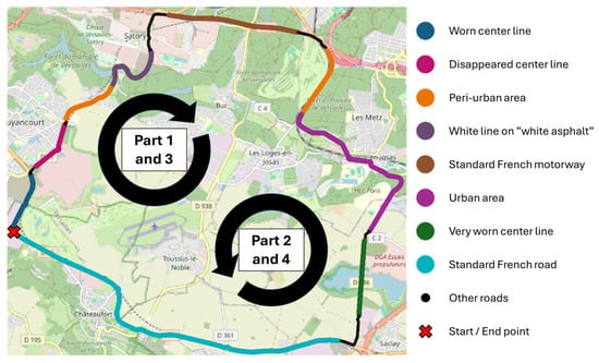
To evaluate the proposed method, the pipeline was applied to a large image dataset acquired on an extensive road circuit (Figure 14). The objective of this acquisition was to collect a large number of images that are as representative as possible of the variety of road scenes around the CORE Center and to capture maximal information from those scenes and road markings. This road circuit was designed to capture both simple and complex scenarios, including worn and severely worn markings, roads without markings, roads with varying pavement colors, roads with heavy shadows on sunny days, and routes in urban or peri-urban areas. Ultimately, we tried to capture all scenarios proposed by Table VIII in the Zhang et al. review [12]. In this dataset, images are organized into four parts corresponding to two round trips.

Figure 14. Road circuit selected to constitute the dataset.

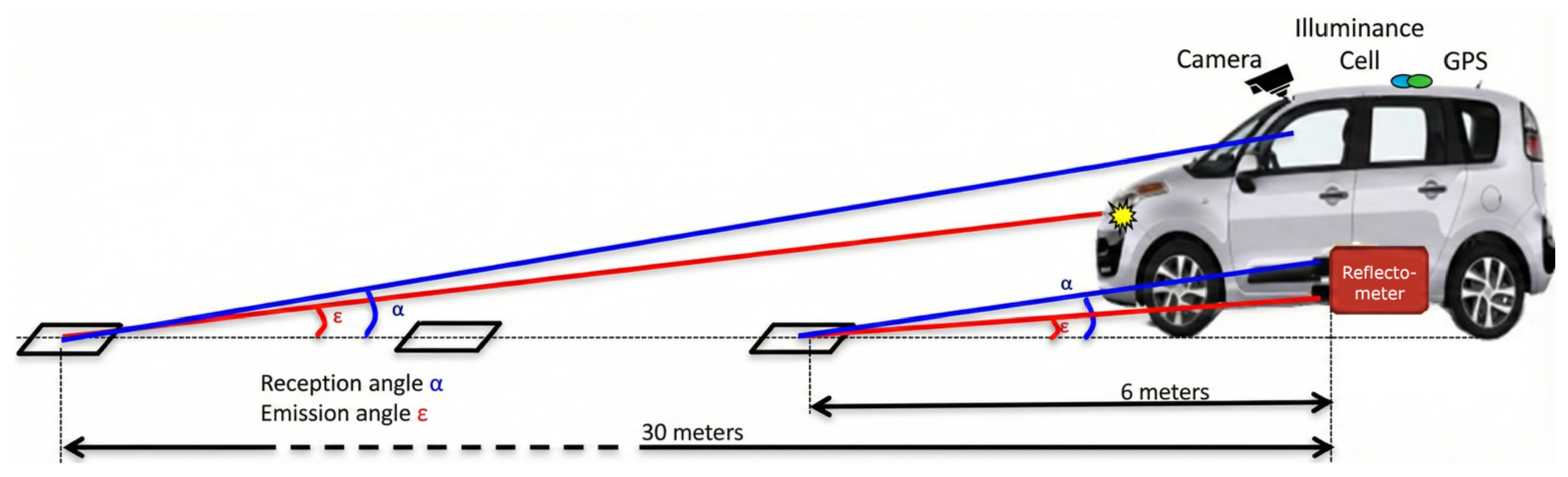
Measures were acquired by the CEREMA of Strasbourg for a COLAS contract. Figure 15 shows the acquisition protocol. Measurement devices consisted of two reflectometers measuring the retroreflectivity and contrast of markings, and an on-board camera to illustrate each measurement. These devices conform to the EN 1436 geometric visibility standard. Only images from the camera are considered here. Each image is geolocalized, captured in full HD 1080p, and acquired in November 2022 under day and dry pavement conditions. The only preprocessing step was to crop the image by two-thirds from the top. Road scenes were sampled at 10 m intervals along the circuit.

Figure 15. Diagram of method’s measurement geometry.

6.2. Road Marking Detections

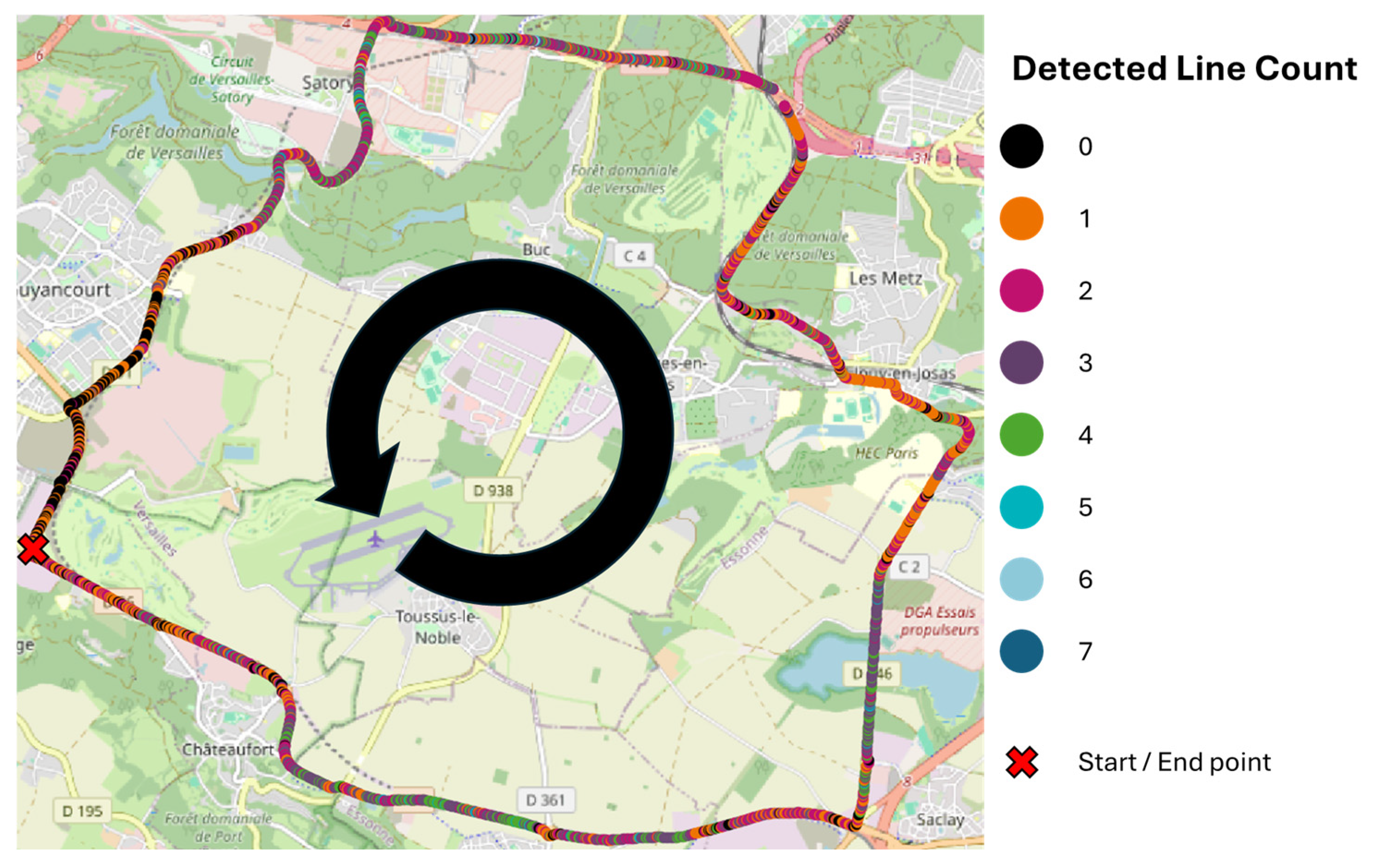
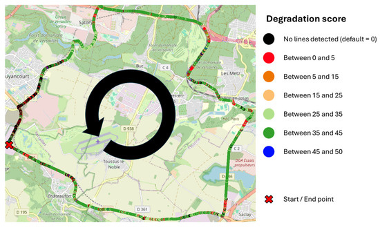
In this section, the results of the detections by YOLOv8 are presented. For example, Figure 16 illustrates the spatial distribution of all line marking detections for part 2. The number of detections varies between 0 and 7 detected lines across 2630 images. Due to the 10 m interval, the map shows a dense sequence of points. On French roads, dashed line road markings are typically applied according to a 13 m sectioning rule, which explains the spatial pattern observed on the map.

Figure 16. The number of detected lines at each GPS coordinate along the road circuit for part 2, with successive points spaced at 10 m intervals.

Table 3 summarizes all detections. A total of 21,497 detections were recorded: 97% correspond to lines, 2% to arrows, and 1% to crosswalks. The large disparity between the count of line markings and that of arrows and crosswalks is attributable to the fact that arrows and crosswalks occur primarily in urban contexts and are rarely or never observed on other road types, whereas line markings are everywhere. Each dataset segment contains a comparable number of detections, except for the third segment, which is shorter due to a camera detachment incident.

Table 3. Number of YOLOv8 raw detections for each road marking class, for each part.

	Line	Arrow	Crosswalk
Part 1	5402	106	65
Part 2	5305	129	79
Part 3 *	4275	107	68
Part 4	5744	139	78
Total	20,726	481	290

* Smaller number of images due to the camera falling off the vehicle at the end of road circuit.

Table 4 reports the Cochran sampling results for each marking class within each dataset part. From the observed detection frequency (p) for a given class, the required sample size is derived. The p-frequency denotes the probability that YOLOv8 detects that class in a randomly selected image, irrespective of detection correctness. For instance, a p-frequency of 0.882 for lines in part 2 indicates that YOLOv8 detects a line in 88.2% of randomly chosen images from that part. From this p-frequency the Cochran sampling is composed of 318 randomly chosen images. Half of them correspond to detected lines, and the other correspond to no line detection. Cochran sampling reduces the number of images requiring manual inspection for lines in part 2 from 2630 to 318, with a 95% confidence level.

Table 4. Cochran sampling for YOLOv8 raw detections for each road marking class, for each part.

	Line		Arrow		Crosswalk
	p-frequency	Sample	p-frequency	Sample	p-frequency	Sample
Part 1	0.9	274	0.028	84	0.023	70
Part 2	0.882	318	0.036	106	0.028	84
Part 3 *	0.898	280	0.037	108	0.031	92
Part 4	0.917	232	0.039	116	0.027	80

* Smaller number of images due to the camera falling off the vehicle at the end of road circuit.

Table 5 presents the number of TP, FP, FN, and the F1-score computed for each Cochran sample. These metrics are based on the manual inspections performed by the assessors. YOLOv8 performance on the road circuit varied from 77% to 96%. On details, the average F1-score by class is: 80% for line, 87% for arrow, and 93% for crosswalk. Arrows and crosswalks are detected more accurately, which can be attributed to their singular shapes and lower prevalence in the road circuit. These results demonstrate that YOLOv8 constitutes an acceptable detector for the subsequent inspection method. Cases where our YOLOv8 fails are few but still occur: it struggles to detect lines located at the far left of the scene; it sometimes confuses parking-slot markings with a discontinuous line; and it can occasionally detect the same marking twice. A RGR score has been established for each image, and it will be shown in the next section.

Table 5. Performances (true positive, false positive, false negative, and F1-score) computed from each manual inspection on Cochran samples for each section of the dataset.

	Line				Arrow				Crosswalk
	TP	FP	FN	F1	TP	FP	FN	F1	TP	FP	FN	F1
Part 1	288	25	66	0.86	44	14	4	0.83	34	3	0	0.96
Part 2	332	58	122	0.79	63	11	2	0.91	38	6	0	0.93
Part 3 *	258	63	56	0.81	59	18	0	0.87	44	6	0	0.94
Part 4	243	26	113	0.77	62	16	2	0.87	35	8	0	0.90

* Smaller number of images due to camera falling off the vehicle at the end of road circuit.

6.3. Random Generated Reference (Line Only)

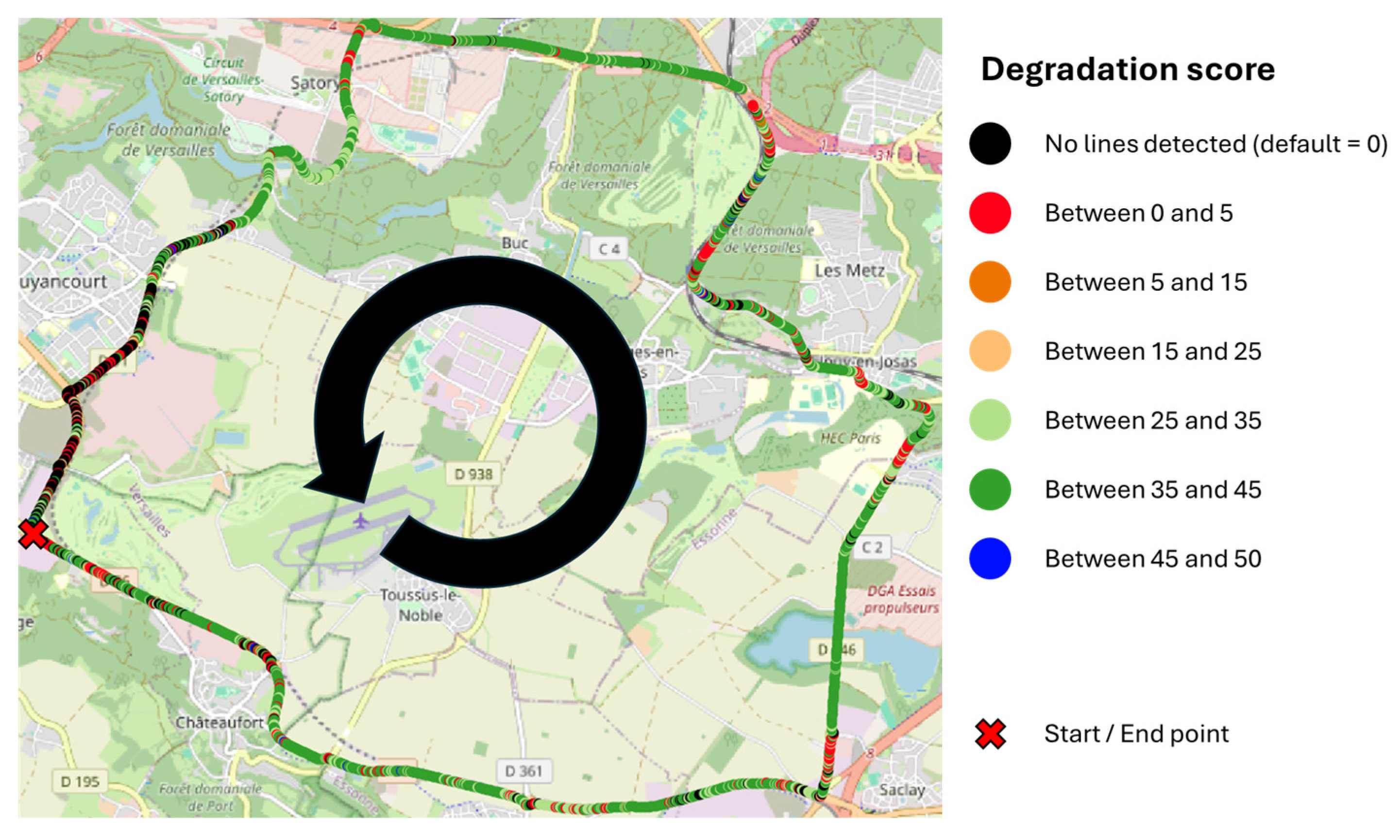
In this section, the results of the RGR scores are presented. For example, Figure 17 illustrates the survey road circuit and the spatial distribution of all line marking inspection scores for part 2. Each RGR class score is present. Table 5 provides a more detailed breakdown of the degradation score frequency for line class, by part. The frequency indicates the probability that at least one detected line in a given part, irrespective of the detection correctness, falls into a specific degradation-score interval. For example, a frequency of 0.58 for part 2 and the 35–45 interval means that a randomly detected line in part 2 has about a 58% chance of having a RGR score between 35 and 45. The N/A entries correspond to scenes in which no line was detected, either because no line was present or because the detection stage failed to detect it. The associated score is 0 by default.

Figure 17. RGR score with successive points spaced at 10 m intervals (line only).

Table 6 reports the frequency of line-marking class for each interval and part of the road circuit. Table 7 reports the Cochran sample size for the line class, stratified by RGR score interval and by part segment. From each p-frequency (Table 6) the Cochran formula yields a required sample size. Unlike the detection-stage sampling, this scheme does not pair positive and negative instances, because such pairing is not meaningful for degradation-score intervals in this study. The extracted samples are then manually inspected by the assessors, substantially reducing their workload; the samples contain only a few hundred images rather than several thousand. Cochran sampling reduces the number of images requiring manual inspection for lines in part 2 from 2630 to 846, with a 95% confidence level.

Table 6. Frequency of line-marking class for each interval and part.

	Line
RGR class	0–5	5–15	15–25	25–35	35–45	45–50	N/A
Part 1	0.1	<0.01	<0.01	0.20	0.56	0.02	0.11
Part 2	0.11	<0.01	0.01	0.17	0.58	0.01	0.12
Part 3 *	0.17	0.03	0.03	0.21	0.36	0.04	0.16
Part 4	0.14	0.02	0.03	0.32	0.38	0.02	0.09

* Smaller number of images due to the camera falling off the vehicle at the end of road circuit.

Table 7. Cochran sample size for the RGR method for line-marking class, for each part.

Line
RGR class	0–5	5–15	15–25	25–35	35–45	45–50	N/A
Part 1	139	3	7	246	378	27	152
Part 2	149	4	11	128	375	12	167
Part 3 *	215	44	47	255	352	66	206
Part 4	188	30	39	333	363	31	126

* Smaller number of images due to the camera falling off the vehicle at the end of road circuit.

The final step consists of measuring the deviation between the RGR score and the CS126 score manually estimated by assessors on the same Cochran samples.

6.4. Differences Between RGR and CS126 Scores

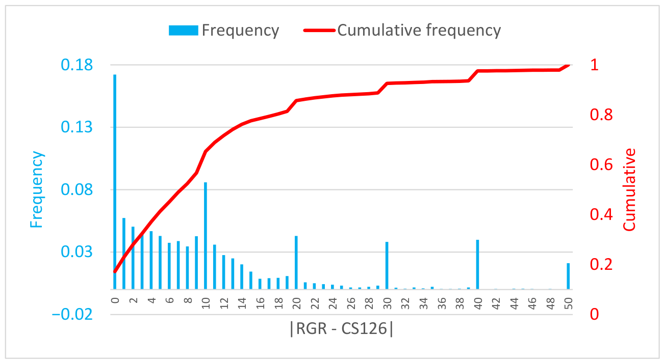
To estimate the differences between the RGR and the assessors’ CS126 scores, several statistical methods can be used. For example, we can report the average error: 10±10. We can also report the correlation between these two scores: 66%, which is encouraging, though not perfect. Another approach would be to establish a linear relationship between the two, which yields an R² of 44%. We have chosen to report in greater detail the distribution of the differences between the two scores.

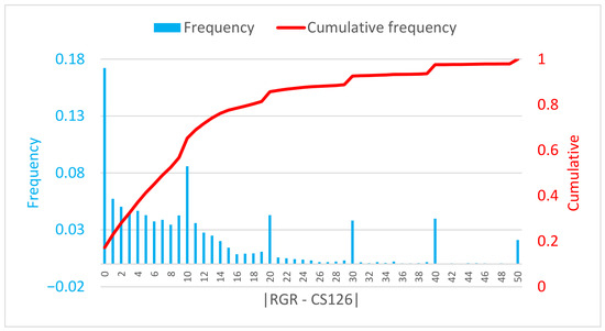
Figure 18 presents the distribution and the cumulative distribution of the differences between the RGR and CS126 scores aggregated over all parts of the circuit. Because assessors were instructed to follow CS126 ratings using discrete increments (0, 10, 20, 30, 40, and 50), while the RGR score is continuous between 0 and 50, it accounts for the peaks observed at those values. The absolute average difference is 10 ± 10 (one ± one CS126 class). In the details, RGR and CS126 scores are equal in 17% of cases; in 68% of cases, error is less than or equal to 10 (one CS126 class); in almost 85% of cases, error is less than or equal to 20 (two CS126 classes); and finally, in the last 15%, error is greater than 20. In operational conditions, the last situation is the most problematic. It usually happens in two specific cases:

Figure 18. The frequency of the differences between the RGR and CS126 scores for all parts of the circuit.

• Our YOLOv8 segmentation can sometimes produce an incorrect mask; for concave-shaped road markings this may lead to an inaccurate inspection as they skip the reconstruction step and only rely on an accurate segmentation process.
• The auto-thresholding step, although generally effective, can fail in specific cases (for example, when markings are extremely degraded or when the pavement has an unusual color).
• A few new road markings in perfect shape can sometimes be missed by Yolov8; in this case, RGR is equal to 0 and the assessors; rating is equal to 50.
• Shadow reconstruction may fail, resulting in an artificially low rating.
• Heavy traffic scenarios can impact the final rating.

Nevertheless, these results are encouraging for an experimental method intended to approximate a standard visual assessment.

7. Discussion

7.1. Road Marking Detection

The detection stage is critical because any error at this step propagates to the inspection stage. Although YOLOv8 is a strong object detector and our Mapillary-trained YOLOv8 reliably detects road markings, it exhibits two practical limitations: the generated segmentation masks lack fine precision (sometimes substantially), and the model occasionally detects pre-markings. These shortcomings must be addressed to maximize the accuracy of the subsequent inspection.

The ideal road marking detector (regardless of the method) would (of course) achieve a perfect recall (no missed markings), avoid detecting pre-markings, and produce perfect pixel-accurate segmentations of detected markings; in practice, this level of performance is difficult to attain. Future work will therefore be to find or create a model meeting the previously discussed properties.

7.2. The Random Generated Reference Methods

The core concept of the proposed approach is to create a virtual reference that can be directly compared with the real road marking. In principle, if one can synthesize an identical road scene—including illumination, cast shadows, weather, traffic and time-of-day conditions—then any marking should be inspectable in any situation, provided the camera can see the marking. In practice, achieving such an exact scene reproduction is challenging; the present method offers an initial, imperfect attempt to bridge that gap.

Several design choices merit discussion. For example, is it necessary to generate a primary reference with spatially varying pixel intensities to mimic the real marking, or would a uniform primary reference (white pixels scaled to the scene illumination) suffice? Once a reference is obtained, must one compute exact per-pixel intensity differences between the real and virtual markings, or is a simpler comparison—for instance, comparing reconstructed pixel counts of the reference and the observed marking [29]—adequate? We contend that accurate per-pixel reconstruction and fine-grained precision are likely essential to robustly inspect markings under diverse conditions. The current implementation has several limitations. The shadow synthesis lacks fidelity; the generated reference tends to be less accurate for concave or complex marking geometries; and the auto-thresholding procedure, although efficient, fails when markings are so degraded that the paint intensity and pavement intensity are nearly indistinguishable.

In this paper, our experiments were conducted exclusively under dry daytime conditions, which is the main reference in the road inspection industry. This choice is due to the fact that other inspection devices than the camera are difficult, or even unsuitable, to use in situations such as rainy weather. However, the study of complex scenarios—including rain, nighttime conditions, or pavement contamination—is planned for future works.

This work should be regarded as a first proof-of-concept that demonstrates the viability of the approach. Future work will focus on rebuilding the reference generation pipeline, moving from conventional image-processing techniques toward a learnable diffusion-based generative model capable of capturing the full variability of road scene conditions.

7.3. Statistical Evaluation and Visual Assessment Standard

To assess the method’s performance, we employed Cochran sampling. This approach is well suited to evaluate the detection stage, since detections can be counted directly. However, it is less appropriate for assessing the inspection stage; applying Cochran sampling to inspection requires discretizing the method’s continuous degradation score into interval classes, which reduces evaluation fidelity. While this procedure is adequate for assessing the current prototype, future work will adopt more appropriate statistical methods to provide a more precise and rigorous evaluation of the inspection stage.

Another major challenge encountered in the evaluation of the inspection method is the absence of established visual assessment standards. We consulted the UK CS126 standard as a reference scale, as it most closely aligns with the objective of our approach. While it would be possible to decouple our degradation score from CS126, we reasoned that aligning with an existing framework would enhance the relevance and comparability of our evaluation and methods.

Despite our efforts to minimize potential bias in the manual inspection of the method’s output, constraints on resources limited our options. The assessors were volunteers drawn from our small team. Although the first author was excluded from the evaluation, the volunteers were not external to the project, which introduces an initial source of bias. A second potential bias arises from the fact that the assessors performed their ratings while aware of the machine-generated score. They were instructed to ignore that score and to evaluate markings according to CS126, but prior knowledge of the automated result may nevertheless have influenced their judgments. We are confident that the assessors did not deliberately replicate the machine score—such behavior would be both counterproductive and unethical—but the mere awareness of the method’s output remains a possible confound.

7.4. Double-Blind Protocol

To reduce bias and strengthen the manual inspection procedure, a double-blind protocol would be preferable: recruiting assessors with no prior knowledge of the study or its outcomes and evaluating the system on a set of road scene samples that were not used during method development. Implementing this approach requires additional time and resources that were not available for the present study; we plan to adopt it in future work, as we fully outlined the procedure:

• Appoint a coordinator responsible for communication with the team members.
• An independent team from our company (and the CY Cergy Paris University) must select a collection of roads representative of France—or even globally, provided the road markings match the geometry represented in the training dataset.
• This same team must carry out video acquisitions under predefined conditions. At this stage, the discussion on viewing angle becomes relevant: if a method is validated on a specific geometry, then assessment must be performed on that same geometry.
• The coordinator receives the videos and must ensure they are anonymized as much as possible to avoid revealing the locations of the roads. This is a complex challenge; for example, road signs can often give clues about the captured road.
• Our team receives the anonymized videos and applies its RGR process to all of them. It also prepares the samples for verification.
• The samples are sent to the coordinator for compliance checks; they are then forwarded to a second independent team that will assess the detection quality and the accuracy of the degradation estimation. This step is also somewhat complex, as the team must receive minimal training in road marking recognition and degradation visualization.
• The coordinator receives the processed samples and measures the differences between the AI results and the verifiers’ results.

At this stage, our solution is a prototype, making it difficult to motivate two independent teams to collaborate with us. In the longer term, we could envision assigning this verification task to a public authority. However, to the best of our knowledge, the concept of verifying AI results after a field operation does not yet have broad consensus.

8. Conclusions and Future Work

This paper presents the initial step toward a complete processing pipeline for detecting and inspecting road marking degradation using a camera mounted on a vehicle. While the detection component is well established within the autonomous vehicle research field, the inspection component remains underexplored today and is essential for road maintenance organizations. The core idea is to generate a virtual reference of the inspected road markings in an ideal state, while reproducing the conditions of the road scene—including illumination, cast shadows, weather, traffic, and time-of-day conditions—so that the real road marking can be compared with the virtual reference. Our method provides a first convergent step toward this concept by producing a reference that aims to respect illumination and shadows.

The innovation of this work lies in the overarching concept of a fully virtual generation that can serve as a perfect reference, enabling the inspection of any road markings under any conditions, provided the camera can observe the marking; and in the integration of the detection and inspection stages, which are often treated separately by researchers, though in practice they are linked, as errors in the first stage propagate to the second. The observed results from this initial draft indicate that we can classify 68% of road markings, across varying conditions, within one CS126 visual assessment class or less. These results were obtained using Cochran sampling and a manual validation of the method’s outputs. While not approaching perfection, the results are encouraging and justify continued development in this direction. We regard this work as a validating proof-of-concept for future efforts.

The next major steps to advance this method are to replace the current reference generation pipeline with a diffusion-based generative model capable of capturing the full variability of road scene conditions; to adopt a more appropriate statistical framework for evaluation; and to acquire, if possible, a dataset evaluating road marking degradation using the CS126 standard as the main metric. This study lays the foundation for our future work in road marking inspection.

References

- Babić, D.; Burghardt, T.E.; Babić, D. Application and characteristics of waterborne road marking paint. Int. J. Traffic Transp. Eng. 2015, 5, 150–169. [Google Scholar] [CrossRef] [Scilit]
- Fiolić, M.; Babić, D.; Gates, T. Road markings and their impact on driver behaviour and road safety: A systematic review of current findings. J. Adv. Transp. 2020, 2020, 7843743. [Google Scholar] [CrossRef] [Scilit]
- Redondin, M.; Bouillaut, L.; Daucher, D. Em approach for weibull analysis in a strongly censored data context-application to road markings. Int. J. Perform. Eng. 2021, 17, 333. [Google Scholar] [CrossRef] [Scilit]
- Dimauro, G.A.; Cafiso, S.; Ghaderi, O.; Pappalardo, G. Development of decay curve for paint pavement marking using machine learning and generalized estimation equation. J. Infrastruct. Preserv. Resil. 2025, 6, 15. [Google Scholar] [CrossRef] [Scilit]
- Sitzabee, W.E.; Hummer, J.E.; Rasdorf, W. Pavement marking degradation modeling and analysis. J. Infrastruct. Syst. 2009, 15, 190–199. [Google Scholar] [CrossRef] [Scilit]
- Charbonnier, P.; Diebolt, F.; Guillard, Y.; Peyret, F. Road markings recognition using image processing. In Proceedings of the Conference on Intelligent Transportation Systems, Boston, MA, USA, 9–12 November 1997; IEEE: Piscataway, NJ, USA, 1997; pp. 912–917. [Google Scholar] [CrossRef] [Scilit]
- Bar Hillel, A.; Lerner, R.; Levi, D.; Raz, G. Recent progress in road and lane detection: A survey. Mach. Vis. Appl. 2014, 25, 727–745. [Google Scholar] [CrossRef] [Scilit]
- Foucher, P.; Sebsadji, Y.; Tarel, J.-P.; Charbonnier, P.; Nicolle, P. Detection and recognition of urban road markings using images. In Proceedings of the 2011 14th International IEEE Conference on Intelligent Transportation Systems (ITSC), Washington, DC, USA, 5–7 October 2011; IEEE: Piscataway, NJ, USA, 2011; pp. 1747–1752. [Google Scholar] [CrossRef] [Scilit]
- Philipp, F.; Schumacher, S.; Tadjine, H.H.; Rojas, R. Real time detection and classification of arrow markings in urban streets. Int. J. Automot. Technol. 2018, 19, 379–386. [Google Scholar] [CrossRef] [Scilit]
- Suchitra, S.; Satzoda, R.K.; Srikanthan, T. Detection & classification of arrow markings on roads using signed edge signatures. In Proceedings of the 2012 IEEE Intelligent Vehicles Symposium, Alcala de Henares, Spain, 3–7 June 2012; IEEE: Piscataway, NJ, USA, 2012; pp. 796–801. [Google Scholar] [CrossRef] [Scilit]
- Hautiere, N.; Labayrade, R.; Aubert, D. Real-time disparity contrast combination for onboard estimation of the visibility distance. IEEE Trans. Intell. Transp. Syst. 2006, 7, 201–212. [Google Scholar] [CrossRef] [Scilit]
- Zhang, Y.; Lu, Z.; Zhang, X.; Xue, J.-H.; Liao, Q. Deep learning in lane marking detection: A survey. IEEE Trans. Intell. Transp. Syst. 2021, 23, 5976–5992. [Google Scholar] [CrossRef] [Scilit]
- Dewi, C.; Chen, R.-C.; Zhuang, Y.-C.; Jiang, X.; Yu, H. Recognizing road surface traffic signs based on YOLO models considering image flips. Big Data Cogn. Comput. 2023, 7, 54. [Google Scholar] [CrossRef] [Scilit]
- Kong, W.; Zhong, T.; Mai, X.; Zhang, S.; Chen, M.; Lv, G. Automatic detection and assessment of pavement marking defects with street view imagery at the city scale. Remote Sens. 2022, 14, 4037. [Google Scholar] [CrossRef] [Scilit]
- Wang, Z.; Ikeura, R.; Hayakawa, S.; Zhang, Z. Road marking damage degree detection based on boundary features enhanced and asymmetric large field-of-view contextual features. J. Imaging 2025, 11, 259. [Google Scholar] [CrossRef] [Scilit]
- Wang, Z.; Ikeura, R.; Hayakawa, S.; Zhang, Z. Evaluation of Pavement Marking Damage Degree Based on Rotating Target Detection in Real Scenarios. Automation 2025, 6, 70. [Google Scholar] [CrossRef] [Scilit]
- El Krine, A.; Redondin, M.; Girard, J.; Heinkele, C.; Stresser, A.; Muzet, V. Does the condition of the road markings have a direct impact on the performance of machine vision during the day on dry roads? Vehicles 2023, 5, 286–305. [Google Scholar] [CrossRef] [Scilit]
- EN 1436:2018; Road Marking Materials-Road Marking Performance for Road Users and Test Methods. European Committee for Standardization (CEN): Brussels, Belgium, 2018.
- CS 126; Inspection and Assessment of Road Markings and Road Studs. National Highways: Birmingham, UK, 2022.
- SS 589:2013 (2022); Specification for Hot-Applied Thermoplastic Road Marking Materials–Materials, Performance and Application. Enterprise Singapore: Singapore, 2022.
- Redmon, J.; Divvala, S.; Girshick, R.; Farhadi, A. You only look once: Unified, real-time object detection. In Proceedings of the IEEE Conference on Computer Vision and Pattern Recognition, Las Vegas, NV, USA, 27–30 June 2016; IEEE: Piscataway, NJ, USA, 2016; pp. 779–788. [Google Scholar]
- Mapillary. Mapillary Datasets. Available online: https://www.mapillary.com/datasets (accessed on 10 April 2026).
- Morrissett, A.; Abdelwahed, S. A review of non-lane road marking detection and recognition. In Proceedings of the 2020 IEEE 23rd International Conference on Intelligent Transportation Systems (ITSC), Rhodes, Greece, 20–23 September 2020; IEEE: Piscataway, NJ, USA, 2020; pp. 1–7. [Google Scholar] [CrossRef] [Scilit]
- Pan, X.; Shi, J.; Luo, P.; Wang, X.; Tang, X. Spatial as deep: Spatial CNN for traffic scene understanding. In Proceedings of the AAAI Conference on Artificial Intelligence, New Orleans, LA, USA, 2–7 February 2018. [Google Scholar] [CrossRef] [Scilit]
- Ghafoorian, M.; Nugteren, C.; Baka, N.; Booij, O.; Hofmann, M. El-gan: Embedding loss driven generative adversarial networks for lane detection. In Proceedings of the European Conference on Computer Vision (ECCV) Workshops, Munich, Germany, 8–14 September 2018. [Google Scholar]
- Zhang, Y.; Lu, Z.; Ma, D.; Xue, J.-H.; Liao, Q. Ripple-GAN: Lane line detection with ripple lane line detection network and Wasserstein GAN. IEEE Trans. Intell. Transp. Syst. 2020, 22, 1532–1542. [Google Scholar] [CrossRef] [Scilit]
- Xiao, D.; Yang, X.; Li, J.; Islam, M. Attention deep neural network for lane marking detection. Knowl. -Based Syst. 2020, 194, 105584. [Google Scholar] [CrossRef] [Scilit]
- Xu, X.; Yu, T.; Hu, X.; Ng, W.W.Y.; Heng, P.-A. SALMNet: A structure-aware lane marking detection network. IEEE Trans. Intell. Transp. Syst. 2020, 22, 4986–4997. [Google Scholar] [CrossRef] [Scilit]
- Hou, Y.; Ma, Z.; Liu, C.; Loy, C.C. Learning lightweight lane detection CNNS by self attention distillation. In Proceedings of the IEEE/CVF International Conference on Computer Vision, Seoul, Republic of Korea, 27 October–3 November 2019; IEEE: Piscataway, NJ, USA, 2019; pp. 1013–1021. [Google Scholar]
- Vokhidov, H.; Hong, H.G.; Kang, J.K.; Hoang, T.M.; Park, K.R. Recognition of damaged arrow-road markings by visible light camera sensor based on convolutional neural network. Sensors 2016, 16, 2160. [Google Scholar] [CrossRef] [Scilit]
- Varghese, R.M.S. Yolov8: A novel object detection algorithm with enhanced performance and robustness. In Proceedings of the 2024 International Conference on Advances in Data Engineering and Intelligent Computing Systems (ADICS), Chennai, India, 17–18 April 2024; IEEE: Piscataway, NJ, USA, 2024; pp. 1–6. [Google Scholar] [CrossRef] [Scilit]
- Haimer, Z.; Mateur, K.; Farhan, Y.; Madi, A.A. Road marking detection and instance segmentation using YOLOv8 models. In Proceedings of the 2024 10th International Conference on Optimization and Applications (ICOA), Almeria, Spain, 17–18 October 2024; IEEE: Piscataway, NJ, USA, 2024; pp. 1–8. [Google Scholar]
- Kulawik, J.; Kuczyński, Ł. AI-Based detection and classification of horizontal road markings in digital images dedicated to driver assistance systems. Appl. Sci. 2025, 15, 12189. [Google Scholar] [CrossRef] [Scilit]
- Bordet, T.; Redondin, M.; Bornhofen, S.; Denaës, S.; Histace, A. Estimating the repeatability and reproducibility of an AI-embedded measuring device: Application to road markings. EPJ Web Conf. 2025, 323, 05001. [Google Scholar] [CrossRef] [Scilit]
- Wen, C.; Sun, X.; Li, J.; Wang, C.; Guo, Y.; Habib, A. A deep learning framework for road marking extraction, classification and completion from mobile laser scanning point clouds. ISPRS J. Photogramm. Remote Sens. 2019, 147, 178–192. [Google Scholar] [CrossRef] [Scilit]
- Dong, Z.; Zhang, H.; Zhang, A.A.; Liu, Y.; Lin, Z.; He, A.; Ai, C. Intelligent pixel-level pavement marking detection using 2D laser pavement images. Measurement 2023, 219, 113269. [Google Scholar] [CrossRef] [Scilit]
- Mahlberg, J.A.; Cheng, Y.-T.; Bullock, D.M.; Habib, A. Leveraging LiDAR intensity to evaluate roadway pavement markings. Future Transp. 2021, 1, 720–736. [Google Scholar] [CrossRef] [Scilit]
- Brinster, G.L.; Hodaei, M.; Eissa, A.M.; DeLoach, Z.; Bruno, J.E.; Habib, A.; Bullock, D.M. Evaluating Mobile LiDAR Intensity Data for Inventorying Durable Tape Pavement Markings. Sensors 2024, 24, 6694. [Google Scholar] [CrossRef] [Scilit]
- Che, E.; Olsen, M.J.; Parrish, C.E.; Jung, J. Pavement marking retroreflectivity estimation and evaluation using mobile LiDAR data. Photogramm. Eng. Remote Sens. 2019, 85, 573–583. [Google Scholar] [CrossRef] [Scilit]
- Burghardt, T.E.; Popp, R.; Helmreich, B.; Reiter, T.; Böhm, G.; Pitterle, G.; Artmann, M. Visibility of various road markings for machine vision. Case Stud. Constr. Mater. 2021, 15, e00579. [Google Scholar] [CrossRef] [Scilit]
- Soilán, M.; González-Aguilera, D.; Del-Campo-Sánchez, A.; Hernández-López, D.; Del Pozo, S. Road marking degradation analysis using 3D point cloud data acquired with a low-cost Mobile Mapping System. Autom. Constr. 2022, 141, 104446. [Google Scholar] [CrossRef] [Scilit]
- Chen, T.; Dai, J.; Dong, B.; Zhang, T.; Xu, W.; Wang, Z. Road marking defect detection based on CFG_SI_YOLO network. Digit. Signal Process. 2024, 153, 104614. [Google Scholar] [CrossRef] [Scilit]
- Wu, J.; Liu, W.; Maruyama, Y. Street view image-based road marking inspection system using computer vision and deep learning techniques. Sensors 2024, 24, 7724. [Google Scholar] [CrossRef] [Scilit] [PubMed]
- Manongga, W.E.; Chen, R.-C. Road marking sign damage detection and classification using deep learning and fuzzy method. IEEE Access 2025, 13, 92943–92952. [Google Scholar] [CrossRef] [Scilit]
- CROW Publication 380. Kwaliteitscatalogus Openbare Ruimte 2018—Standaardkwaliteitsniveaus voor Onderhoud; CROW: Ede, The Netherlands, 2018. (In Dutch) [Google Scholar]
- Mapillary. Mapillary Research. Available online: https://research.mapillary.com/ (accessed on 10 April 2026).
- Otsu, N. A threshold selection method from gray-level histograms. Automatica 1979, 11, 285–296. [Google Scholar] [CrossRef] [Scilit]
- ISO/CIE 11664-4:2019; Colorimetry—Part 4: CIE 1976 L*a*b* Colour Space. International Organization for Standardization (ISO): Geneva, Switzerland, 2019.
- International Electrotechnical Commission (IEC). Homepage. Available online: https://www.iec.ch/homepage (accessed on 10 April 2026).
- IEC 61966-2-1:1999; Multimedia Systems and Equipment-Colour Measurement and Management—Part 2-1: Colour Management-Default RGB Colour Space-sRGB. International Electrotechnical Commission (IEC): Geneva, Switzerland, 1999.
- International Commission on Illumination (CIE). Available online: https://cie.co.at/ (accessed on 10 April 2026).
- CIE S 014-1:2006; Colorimetry—Part 1: CIE Standard Colorimetric Observers. International Commission on Illumination (CIE): Vienna, Austria, 2006.
- ISO/CIE 11664-2:2022; Colorimetry—Part 2: CIE standard illuminants. International Organization for Standardization (ISO): Geneva, Switzerland, 2022.
- ITU. BT.709: Parameter Values for the HDTV Standards for Production and International Programme Exchange. Available online: https://www.itu.int/rec/R-REC-BT.709 (accessed on 10 April 2026).
- Cochran, W.G. Sampling Techniques, 3rd ed.; John Wiley & Sons: New York, NY, USA, 1977. [Google Scholar]
Disclaimer/Publisher’s Note: The statements, opinions and data contained in all publications are solely those of the individual author(s) and contributor(s) and not of MDPI and/or the editor(s). MDPI and/or the editor(s) disclaim responsibility for any injury to people or property resulting from any ideas, methods, instructions or products referred to in the content. |
© 2026 by the authors. Licensee MDPI, Basel, Switzerland. This article is an open access article distributed under the terms and conditions of the Creative Commons Attribution (CC BY) license.