Abstract
Despite significant advancements in Artificial Intelligence, its widespread adoption in the clinical domain remains restricted due to the inherent complexity, fragmented nature, and diversity of healthcare systems. Each healthcare provider has unique data, clinical guidelines, data availability, system architectures, heterogeneity, and distribution. These challenges hinder the application of Clinical Decision Support Systems because of a limited understanding of how existing systems can be effectively redeployed across different healthcare providers. Redeployment is needed because it enables the reuse of existing knowledge, maximizes reusability, and avoids code duplication, thereby reducing the costs, effort, and time required to develop the Clinical Decision Support System from scratch. In addition, it ensures faster deployment and wider accessibility in the case of resource-constrained healthcare providers. An essential for redeployment is to identify the possible situations in which variables differ between two dynamic environments. To address this gap, we propose a structured multi-dimensional framework that systematically analyzes the potential differences between the variables. To represent the output of differences across dimensions based on variables in a systematic, machine-readable manner, we proposed a conceptual model, “VarDiff”, and a decision matrix of possible outcomes across five differential dimensions. This conceptual model provides a systematic, structural, and logical representation of a multidimensional framework for identifying differences among variables across data ecosystems. It formalizes variable characteristics in terms of semantic entities to observe differences among variables. The adaptation categories help identify the specific adaptation type, enabling the selection of relevant adaptation strategies in the “Mutator” component.
1. Introduction
Computer-based Decision Support Systems (DSS) in the clinical domain have evolved continuously over five decades, yet their applications remain limited. This is mainly due to the complexity of healthcare providers, in which each ecosystem has a unique architecture characterized by heterogeneity, workflows, protocols, knowledge representation, and data availability. These complexities pose substantial barriers to the seamless redeployment of a Clinical Decision Support System (CDSS) [1] across ecosystems, such as from one healthcare provider to another. The redeployment of CDSS is crucial because it leverages the reference to existing knowledge and infrastructure from the healthcare provider on which a CDSS is trained, rather than designing a new CDSS from scratch for another healthcare provider. Using redeployment, healthcare providers can minimize manual effort in re-engineering and maximize the reusability of code and implementation approaches, leading to faster deployment timelines, reduced costs and time, and improved interoperability between healthcare providers [2]. In addition, the redeployment is needed when resource-constrained providers cannot afford to build their own models from scratch. Hence, redeployment poses a major challenge to the successful implementation of Artificial Intelligence (AI) [3,4,5,6] in healthcare. Redeployment of a complex AI solution requires understanding the differences in variables between two healthcare providers [7]. Any differences in variables may have adverse effects on the performance of the CDSS [8]. The cost of rebuilding a CDSS from scratch in a new ecosystem can be substantially high [9] because it requires a combination of medical knowledge and data-science knowledge [10,11]. Moreover, the training and labeling of data for developing a complex AI solution may require significant time and manual effort [12,13,14]. Due to a lack of knowledge on how to identify and determine the differences between the variables of both ecosystems [1]. Furthermore, there is limited guidance on how to structurally represent [15,16,17,18,19] the output of these differences in a machine-readable form. Therefore, identification of possible differences between the variables in each dimension is important for planning the relevant adaptation strategies according to the adaptation type. Each type of difference requires a distinct adaptation strategy, and planning adaptation strategies for redeploying a CDSS across healthcare providers requires both data science and medical knowledge.
In our earlier work, we proposed a framework to support the redeployment of complex CDSSs across healthcare providers and called it “Adaptive Semantic Framework (ASF)” [1], where three main components were discussed: the “Differentiator”, “Mutator”, and “Validator”. ASF identifies differences between the variables of source and target ecosystems by leveraging domain ontologies using the “Differentiator” component and generates candidate CDSSs through a “Mutator” component by applying the possible adaptation strategies, which are then evaluated by a “Validator” component.
In this paper, we present each differential dimension in detail, describe the possible outcomes for each dimension, introduce a conceptual model, “VarDiff”, to represent differential knowledge, and provide a workflow illustrating how these outputs can be utilized within the “Mutator” component. This work establishes a conceptual and logical foundation for the identification and categorization of variable-level differences in CDSS redeployment. These differences provide structured inputs to support adaptation decisions within the “Mutator” component, indicating which variables can be reused directly and which require adaptation to the target data ecosystem.
It is important to note that this work does not present a fully automated or end-to-end redeployment system. Instead, it establishes a structured framework for difference identification and categorization between the variables of two dynamic healthcare providers, which can support future development of semi-automated adaptation systems.
For clarity, we define key terms used throughout this paper. The term “Redeployment” refers to the process of transferring an existing CDSS from a source healthcare provider to a target healthcare provider. “Reusability” refers to the ability to reuse existing models, knowledge structures, or components in another system or application. Finally, the term “Adaptation” refers to the set of modifications required to ensure that the redeployed CDSS functions correctly in the target healthcare provider.
The paper is structured as follows: Section 2 presents the problem statement. Section 3 highlights the related work on the comparison of datasets and similarity analysis. Section 4 explains the utility of differential dimensions using a general scenario. Section 5 contains the overall workflow of the Structured Multi-Dimension (SMD) Framework. Section 6 explains the matching possibilities of each dimension. Section 7 represents the conceptual model named “VarDiff” of the output of differences across five dimensions. Section 8 includes the possible outcomes of differences based on the combination of possible matches from each dimension through a logical decision matrix to categorize into adaptation categories. Section 9 explains the role of the mutator after categorizing the adaptation scenarios based on dimension outcomes. Section 10 represents a case study on the SMD framework and how it will identify the adaptation categories based on the outcomes from each dimension. Finally, Section 11 highlights our contributions to the challenge of redeploying a CDSS across healthcare providers and outlines future scope.
2. Problem Statement
2.1. Problem Overview
Redeploying a CDSS from one healthcare provider to another is challenging due to variability in the source and target data ecosystems. Suppose a source healthcare provider and a target healthcare provider each maintain their own data ecosystems, variable definitions, metadata, and patient population characteristics.
The redeployment problem can therefore be formally defined as follows:
- Let us assume a CDSS D that operates in environment using input variables , where is the set of used variables and is the set of visible variables of . Then determine how to construct an adapted CDSS that operates in environment using input variables , such that the behavior of sufficiently approximates the behavior of . Here, the “sufficiently approximates” refers to maintaining the structural consistency using structure learning scoring functions [20], the strength of association between the nodes or concepts through Conditional Probability Table (CPT) [21] supported by clinical evidence, and maintaining overall performance with less deviation relative to the source CDSS.
The redeployment of an existing CDSS from the source environment to a target environment may have the following challenges due to differences in variables:
- Fragmented and highly variable data environments across different healthcare providers.
- Differences in variable meaning or context.
- Differences in representation, such as formats, units, precision value, and category.
- Differences in metadata such as measurement device, sampling method, clinical workflow, and patient state.
- Differences in statistical distributions such as normal, Poisson, chi-square, and F-distribution.
2.2. Assumptions on Both Environments
Here, we assume the source environment provides a set of variables:
The CDSS uses a subset of these variables as input:
The target environment provides its own set of variables:
and
Similarly, is a CDSS on
2.2.1. Assumptions on Data Dictionaries
We assume that both providers may have machine-processable data dictionaries that include variable labels, data types, units, ranges, definitions, measurement context (device, sample, type, and timing), coding schemes, and other explicit details. For example, a variable called “Systolic Blood Pressure” having a label of “SBP”, a data type of “numeric integer”, a unit of “mmHg”, a valid range from “50 to 250”, a clinical definition of “maximum arterial pressure during cardiac contraction”, a measurement device details with the code “automated sphygmomanometer”, a measurement timing with the code “at admission”, and a coding scheme with the code “local hospital code” or “Systematised Nomenclature of Medicine-Clinical Terms (SNOMED-CT) [22] concept identifier”.
In practical healthcare applications, data dictionaries and metadata are often incomplete, and mappings between variables and ontology concepts may be ambiguous, missing, or one-to-many. To address these challenges, the proposed framework incorporates a staged fallback strategy. First, the variables used by the source CDSS (referred to as “used variables”) are standardized using a primary clinical terminology, such as SNOMED-CT, to alleviate semantic ambiguity. If no direct match is found, the framework uses crossterminology or meta-thesaurus references, such as UMLS. For one-to-many mappings, a ranking-based decision rule is used to select the most appropriate concept considering semantic similarity. If automated mapping remains uncertain due to missing definitions or incomplete metadata, human intervention may be required. Finally, if no reliable semantic correspondence can be identified, then the omission of that variable would be referable from the adaptation process. Once the “used variables” are standardized, the framework records metadata differences along with other differences between the source and target ecosystems, which are then used to guide adaptation strategies for CDSS redeployment. In this work, SNOMED-CT is used as the primary terminology for standardizing the “used variables” of the source ecosystem, and the other cross-terminologies will be used in future work.
2.2.2. Assumptions on Variables
Each variable is assumed to be well-defined and characterized by a tuple
where l denotes the label or identifier, represents the data type, d is the value domain (range or categorical set), u denotes the unit of measurement, m represents the measurement context (e.g., device, timing, measure actors, and situations, etc.), and denotes the empirical data distribution associated with the variable.
These variable characteristics support the structured comparison across ecosystems, including label-level alignment, semantic alignment, representation-level comparison, metadata-level comparison, and data-level statistical comparison.
2.2.3. Assumptions on Ontological Structure
Medical ontologies [23] give a standardized representation of clinical knowledge that encompasses concepts, Unique Concept Identifiers (UOI), taxonomy classifications, logical relationships, synonym information, well-defined clinical terms, etc. The medical ontology provides a structured semantic foundation that supports interoperability and concept-level alignment among healthcare providers. With the help of clinical domain-based ontologies, such as SNOMED-CT, concept-level normalization and formal semantic alignment of ecosystem variables are enabled. By mapping input variables to SNOMED-CT terms or concepts, this approach ensures consistent interpretation, strengthens deep-match evaluation, and supports surrogate identification for CDSS redeployment. In cases where any variable cannot align with the terminology, we will either reference existing terminology in the future or maintain a human-in-the-loop for manual reconciliation.
Hence, we assume a medical ontology O capturing the clinical concepts associated with all variables in . Each variable corresponds to a unique concept :
3. Related Work
The increasing prevalence of Electronic Health Records (EHR) has led to significant interoperability issues [24] across multiple levels, including structural, semantic, contextual, and metadata dimensions, as well as variations in variables and values. Most existing research has examined approaches to address interoperability and dataset-comparison challenges between the two organizations. However, these studies explore different aspects of the problem, including dataset similarity analysis, ontology-based semantic interoperability, schema-matching mechanisms, and terminology mapping. For a better understanding of the existing literature, we classified it into four categories: (1) ontology-based semantic interoperability approaches, (2) schema matching and data integration frameworks, (3) numerical and unit standardization, and (4) dataset comparison and statistical similarity methods. The following subsections discuss these categories in detail and highlight their limitations with respect to the CDSS redeployment problem.
3.1. Ontology-Based Semantic Interoperability Approaches
We focus on how ontology-based semantic integration techniques enhance interoperability between the two ecosystems. In 2015, Liyanage et al. [25] explored how ontologies can enhance semantic interoperability in healthcare systems characterized by fragmented and heterogeneous data sources, addressing the limitations of traditional standards and terminologies like HL7, ICD, and SNOMED-CT. This study addresses interoperability issues across clinical, public health, and social datasets and, accordingly, applies Semantic Web standards such as RDF, OWL, and SPARQL to formalize semantic meaning and enable consistent data interpretation. The work is valuable in providing a systematic approach to semantic alignment across healthcare organizations using ontology-driven integration, but it did not discuss interoperability regarding variable characteristics, such as units, variable source level, and distribution level. In 2016, Legaz-García et al. [26] described an OWL-based framework that leverages EHR and Semantic Web technologies to enable interoperability and secondary use of clinical data. This framework has been implemented in the Archetype Management System (ArchMS). It demonstrated how Semantic Web technologies can harmonize heterogeneous clinical data formats and support both primary care and secondary analytics. They primarily focused on representation and metadata dimensions to understand semantic and structural alignment but did not provide details on other dimensions that may exist across the ecosystems. In 2025, Ambalavanan et al. [27] discussed the significance of ontologies as a bridge between AI and healthcare providers. They focused on how the ontology-enabled frameworks provide a structured representation of clinical knowledge to enhance semantic interoperability among healthcare providers. After standardizing clinical concepts, relationships, and terminologies, the ontology can support advanced AI applications, such as CDSS, NLP, and predictive analytics. Authors also discussed how ontology-based systems help address challenges posed by fragmented data and inconsistent terminologies across healthcare providers and highlighted the limitations of semantic mismatches between existing standards, such as SNOMED CT and HL7 FHIR. However, they emphasized the significance of ontology integration but did not discuss other dimensions of difference, as semantic integration poses challenges for information exchange.
These methods, as reported in the literature, provide mechanisms for achieving semantic alignment across healthcare and enable knowledge integration through ontology-based frameworks. Still, their attention remains primarily on semantic interoperability and structural data harmonization, without considering additional factors such as variable representation formats, measurement context, metadata differences, or shifts in statistical distributions. Our proposed framework extends beyond semantic alignment by enabling a multi-dimensional differential analysis that identifies differences across semantic, structural, representational, contextual, and statistical dimensions, thereby supporting CDSS redeployment.
3.2. Schema Matching and Data Integration Frameworks
Several studies have explored schema matching methods and data integration frameworks for matching datasets across heterogeneous healthcare providers. In 2020, Tao et al. [28] introduced an Interactive Mapping Interface (IMI), a web-based tool designed to improve semantic interoperability by mapping healthcare data dictionaries to biomedical ontologies using a fuzzy mechanism. The study aimed to design, implement, and test IMI as a general-purpose ontology mapping system with three modules: ontology library, interactive interface, and recommendation engine, using Ruby on Rails. The main focus of this work was on collaborative workflows, semantics, metadata, and scalability in healthcare data harmonization using an ontology.
In 2021, Burse et al. [29] highlighted that healthcare interoperability has remained an unresolved challenge since the 1980s, with previous existing customized solutions being unable to provide a scalable framework. They presented a multi-level view of interoperability, encompassing syntactic, semantic, and structural discrepancies, as well as medical ontologies that support semantic harmonization. The authors observed that the semantic web technologies, including RDF, OWL, and linked data principles, can strengthen interoperability by enabling machine-interpretable meaning. The authors provided an interoperability approach for the semantic and syntactic dimensions of overall health information exchange but did not provide any details on variable-level comparison across representation, metadata, and data levels.
In 2021, Koutras et al. [30] introduced an open-source framework, Valentine, for evaluating schema-matching algorithms used in dataset discovery and integration. They assessed the performance of seven schema-matching techniques across four dataset relationships: unionable, view-unionable, joinable, and semantically joinable. It is useful for CDSS redeployment research, as it guides the selection of matching algorithms for aligning heterogeneous healthcare datasets and managing semantic and metadata variability across organizations, but it does not account for ontology-driven evaluation and has limited applicability to hierarchical or clinical terminologies such as SNOMED-CT and LOINC.
In 2022, Stroganov et al. [31] addressed interoperability challenges in the UK Biobank arising from heterogeneous terminologies by mapping Read v2/v3 codes to ICD-9/10 and SNOMED CT. They used 123 million GP records to assess mapping accuracy and found it to be limited, with 33.4% imprecise and 5.9% multiple mappings due to structural and semantic mismatches. Moreover, they observed that an automated approach alone was insufficient for precise mapping and that mapping accuracy improved when they combined the fuzzy string matching mechanism with expert validation. However, the study did not discuss any structural approach to identifying differences between the variables. Compared to our work, they did not discuss representation differences, metadata variation, or cohort-level distributional analysis, which reduces its applicability to multi-dimensional CDSS redeployment.
In the same year, Matentzoglu et al. [32] introduced Simple Standard for Sharing Ontological Mappings (SSSOM), a FAIR-compliant standard designed to address existing challenges in ontology and terminology mapping, particularly the lack of semantic precision, provenance, and transparent metadata. The framework provided a simple, extensible tabular schema that supports explicit mapping types, confidence scoring, and governance mechanisms, enabling reproducible and interoperable data integration across biomedical systems. They worked on the label mapping using the terminology and provided a confidence score for accurate mapping, but they did not address other mapping dimensions.
In 2022, Mello et al. [33] conducted a literature review to examine the state of semantic interoperability in EHR standards, addressing fragmentation and heterogeneity in HIS. The authors identified key standards, terminologies, and technologies used to achieve interoperability through openEHR, ISO 13606, HL7 CDA/FHIR, terminologies such as SNOMED-CT, LOINC, and ICD-10, and semantic web tools such as OWL, RDF, and SPARQL. It introduces a taxonomy of five interoperability dimensions—standards, terminologies, semantic tools, data storage, and evaluation methods. This study is valuable for the data exchange and secondary EHR use by combining standards and semantics. They focused on label matching and semantic mapping of variables to terminology terms or concepts but did not address meta-context, representation, or distribution-level mappings for more accurate data exchange across healthcare systems.
Moreover, from the literature, we observed that many researchers have investigated methods for determining similarity and dissimilarity among concepts [34,35,36,37,38] within or across healthcare providers. Their focus has primarily been on the dimension of semantic similarity, without considering all possible dimensions of differences. Furthermore, no prior work has addressed cross-organizational applications for determining similarity or dissimilarity across syntactic, semantic, representational, contextual, and value dimensions. Moreover, no one has proposed a structural approach to determine differences between variables across two healthcare providers and to represent them formally.
3.3. Numerical and Unit Standardization
In 2021, Bietenbeck and Streichert [39] highlighted the need to enhance standardized, machine-readable laboratory reports for data exchange among healthcare providers. The authors also discussed that semantic interoperability can be achieved by leveraging the medical terminologies such as LOINC, SNOMED-CT, Unified Code for Units of Measure (UCUM), and Nomenclature for Properties and Units (NPU) [40]. They worked on the standardization of medical numerical records according to the UCUM but did not provide knowledge of unit conversion or other value attributes of variables. Moreover, they did not work on the identification and representation of other differential dimensions. In 2022, Vogl et al. [41] proposed LUMA, a unit mapping and conversion tool that integrates LOINC with UCUM. This tool was designed to facilitate the standardization of laboratory measurement units associated with LOINC-coded tests. The authors observed that although LOINC has been widely adopted for identifying laboratory tests, the related unit standard UCUM has experienced slower adoption due to the complexity of mapping local proprietary units. To address this challenge, the LUMA tool established a formal relationship between LOINC properties and UCUM unit representations using the HL7 FHIR framework. By leveraging the property axis of LOINC codes and linking them to canonical UCUM unit representations, the LUMA tool standardized units and enabled automated unit conversions. The author provided a mapping tool using LOINC and UCUM for automatic unit-of-measurement conversion but did not provide conversion or standardized guidance on managing representation discrepancies, such as value scale, data type, and range.
In 2025, Muñoz Monjas et al. [42] addressed the issue of semantic interoperability in healthcare by focusing on the harmonization of laboratory measurement units across heterogeneous clinical data sources or reports. The authors proposed a dimensional analysis based approach to standardize laboratory units using the UCUM. The authors tested this method on real-world clinical data from the TriNetX research network, and the results demonstrated that the proposed method significantly improves unit standardization, achieving over 90% coverage of laboratory data according to the UCUM. However, they focused on the standardization of medical numerical records using UCUM but did not provide guidance on converting other attribute values of a variable, such as type, format, and value scales.
From this literature review on the standardization of numerical values, we observed that the focus was limited to the conversion or mapping of measurement units and the standardization of laboratory reports. In particular, existing work does not capture all possible attribute-based differences between two healthcare providers, such as the variable’s data type, value scale, and interval range. In addition, they did not address the differences in knowledge among the variables arising from semantic representations, metadata definitions, and data distributions. To address these limitations, our work introduces an SMD framework that captures multidimensional differences and provides a formal representation and, where appropriate, numerical standardization based on the variable’s attributes.
3.4. Dataset Comparison and Statistical Similarity Approaches
In 2015, Maillet et al. [43] introduced the COmpare Multiple METagenomes (COMMET) method for efficiently comparing multiple metagenomic datasets. It can compute intersections between datasets and perform logical operations on read subsets. The method produces similarity matrices, heatmaps, and dendrograms to visualize relationships between samples. The authors are limited to providing an efficient method for computing global similarity across metagenomic datasets using statistical analysis. In the same year,
In 2016, Raff and Jin [44] proposed a Difference-of-Datasets (DoD) framework. It is a statistical method for comparing two datasets to assess their differences. The method involves converting data to binary format, aggregating it to an independent level (e.g., user-level), conducting two-sample Z-tests to compare distributions between datasets, and ranking metrics by Z-score to identify the most significant differences. The authors are limited to identifying similarities between two datasets, considering only two differential scenarios, namely data representation and statistical analysis.
From the literature, it can be observed that existing approaches address interoperability and semantic challenges more than other dimensions, such as statistical dataset comparison, representation matching across all possible attributes of a variable, or metadata dimensions. However, none of these approaches provides a systematic framework for analyzing and representing multi-dimensional differences between variables between healthcare providers. Another gap is evident in the literature: several researchers have addressed numerical standardization and unit conversion, but they have not provided all the details of the possible attributes of variables across the two healthcare providers or how to achieve the standardization. In particular, the combined comparison of syntactic labels, semantic definitions, representation formats, metadata context, and statistical data distributions remains largely unexplored and does not provide guidance on how to formally represent the difference between variables once it is identified.
The main objective of this paper is to provide a conceptual and logical foundation for identifying and categorizing differences between healthcare providers, and representing them in a formal, structured, and machine-readable form. It also defines the variable characteristics required to identify differences within a multi-dimensional framework. Accordingly, we propose five structured dimensions to analyze differences between variables across ecosystems: label (syntactic level), definition (semantic level), representation (units of measurement), metadata (measurement methods and reference ranges), and data (distributional characteristics). In addition, each dimension category comprises several possible differential scenarios that provide knowledge for devising the relevant adaptation strategies, whether they require domain or data science knowledge.
4. General Scenario Based on Differential Dimensions
Figure 1 represents five differential dimensions between two ecosystems Es and Et of two healthcare providers. The main functions of these dimensions are to identify potential differences between the variables of Es and Et, which help in the redeployment of existing CDSS that are trained and run on the source data ecosystem, using the “Used Variable”. To this end, we proposed a Structured Multi-Dimension (SMD) framework that provides the variable difference between Es and Et using a multi-dimensional approach. Since the characteristics of a variable are conceptually orthogonal (independent), any observable variable must be decomposed into structural, semantic, representational, contextual, and statistical components to enable systematic understanding of differences among ecosystems. Therefore, the five dimensions form a collectively exhaustive set of possible divergences relevant to CDSS redeployment. We explain the utility of each dimension for finding the match/nomatch of variables based on label, semantic, value scale, measure scale, and distribution level as follows:
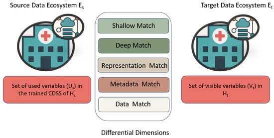
Figure 1.
Differential dimensions between two data ecosystems Es and Et.
- Shallow Match: Differential analysis based on the domain terminology/ontology, such as SNOMED-CT [45], wherein the matches are to be done between the input variables of the source system and the terms in the SNOMED-CT. For each input variable of the Es, look for its representation in the terminology, and then the extracted related terms for each input variable from the terminology will be called “Potential Set”. Then the “Potential Set” will be matched with the variables available in the Et.
- Deep Match: Differential analysis based on the definition of the concept [46] of source system and target system. In the Shallow Match, the differential analysis is performed on the label between the input variables and the terms in the terminology. Thus, it does not provide sufficient information to establish the equivalence of each concept between the source and target systems. In many cases, a term may exhibit homonymy, meaning the same term has different meanings or multiple definitions. The Deep Match ensures that the two systems share a similar concept.
- Representation Match: Differential analysis at the representation level examines how variables are expressed across data ecosystems, focusing on differences in units of measurement (UoM), range, value formats, and textual representations. For units of measurement, the analysis checks whether variables are recorded using the same units or different ones. Value format analysis determines whether differences in representation (for example, integer, decimal, categorical, or encoded values) exist and whether these formats are directly convertible, convertible with some loss of information, or not convertible at all.Finally, the analysis evaluates whether values include textual information (such as clinical notes or qualitative descriptors) and assesses how such text-based values can be reliably transformed into numerical representations for subsequent processing and analysis.
- Metadata Match: Differential analysis at the metadata level checks the differences in how variables are collected or measured across data ecosystems. This analysis considers several metadata-based characteristics, including data collection methods, personnel involved in sample measurement, devices or instruments used, measurement time, sample types, and the clinical context in which the sample was collected. Even when conceptual and representational alignment exists, differences in metadata can alter clinical meaning and impact the quality of care. Incorporating detailed metadata prevents false equivalence, preserves measurement standardization, and supports safe and more precise readjustment across heterogeneous healthcare environments.
- Data Match: Finally, the data match identifies distribution-level differences between source and target variables across data ecosystems. This analysis examines variations in patient mix, including differences in age, gender, disease conditions, and cohort granularity. In addition, distributional differences can arise from missing values, depending on the missingness pattern. These distributional differences can affect the degradation of the performance and reliability of a CDSS. To ensure that the model remains valid and appropriate after the redeployment, it is important to understand the distribution graphs for precise and planned redeployment.
5. Workflow in SMD Framework
Figure 2 illustrates the overall workflow of the proposed Structured Multi-Dimension (SMD) framework, wherein the differences are initiated and traversed through a sequence of five proposed differential dimensions, such as Shallow, Deep, Representation, Metadata, and Data, to systematically identify the differences between a set of variables Es and Et. The main function of the “Differential Condition” is to identify matches/mismatches between source and target variables. The SMD framework is useful for data scientists, clinical informaticians, CDSS vendors, and local health networks that need to port an existing clinical decision support system to a new hospital. By systematically identifying differences between the source and target systems, this framework helps determine whether and how an existing CDSS can be reused, thereby minimizing manual re-engineering, reducing the risk of mis-specification, and speeding up adoption. Redeploying CDSSs often requires manual mapping of hundreds of variables across two data ecosystems, but the SMD framework aims to automate much of this work. Automating the matching steps accelerates redeployment by detecting differences and, accordingly, applying adaptation strategies, whether these require data science, domain expertise, or a hybrid approach. When differences or mismatches persist, the intervention of human experts is required. In the visual flow, red lines represent conditions that return false (meaning a mismatch), which are stored in a common database and require further reconciliation for needful readjustment; green lines represent conditions that return true (meaning a match), and the blue line indicates the starting point of “Difference Condition”.
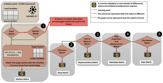
Figure 2.
Overall workflow of Structured Multi-Dimension (SMD) framework.
The framework begins by assessing whether the variables of Es and Et belong to the same terminology. Here, we choose SNOMED-CT due to its richness and comprehensiveness in clinical vocabularies. The Shallow Match has two steps; in the first step, a direct match between source variables and standardized terms in the terminology is identified [47]. For example, the input variable “Body Mass Index” has a direct match in the terminology (SNOMED-CT). If no match is found, approximate string-matching techniques, such as Levenshtein Distance [48], Jaro–Winkler, and fuzzy-logic are employed to find synonyms or conceptually similar terms from the terminology. For calculating the embedding similarity score [49], a pre-built, trained language model on clinical terms is used to determine the similarity score between input variables and terms in terminologies such as ClinicalBert [50] and SNOMED2VEC [51]. For instance, inputs such as “HDL” and “Fasting Blood Sugar” are mapped to their equivalents in the terminology (SNOMED-CT), namely “High-Density Lipoprotein” and “Fasting Blood Glucose”, respectively. Hence, in the first step, we select the potential set of variables in the source system that are relatively similar to the corresponding term in the terminology. In the second step, each variable in the potential set is checked against the variables of the target system. If there is a match, then it will match the definition of both variables in the Deep Match by integrating the natural language model on the associated data dictionary and medical-trained Large Language Model (LLM) [52,53,54]. Next, the Representation Match identifies syntax differences such as unit conversions, range intervals, and textual to numerical conversions with the help of logical operators. The MetaData Match identifies differences in the methods used to collect health data. Last, Data Match assesses the statistical distributions of variables between both systems. For example, skewed age distributions or gender imbalances can significantly affect model performance and bias. Here, we use statistical measures (mean, median, KS-test, chi-Square, and P-test) and divergence metrics (e.g., KL divergence, Jensen–Shannon divergence, and Wasserstein distance) to quantify differences in distributions. Visual techniques (e.g., histograms and Q-Q plots) can be used to visualize distributional shifts resulting from human intervention.
6. Matching Possibilities in Each Dimension
Figure 3 delineates the dimension categorization with their objectives. This top-down sequential approach proceeds from Shallow Match to Data Match to identify differences across dimensions. The dimensional order starts with the Shallow Match because it is necessary to first match the variables of the source system with the terms in the given terminology. After this, we can check the definitions in the Deep Match for the matched variables or the resulting variables from the source system against the target system. Once the definitions are confirmed, we can proceed with the Representation Match to align units of measurement, value ranges, and format conversions (e.g., from textual to numerical data).
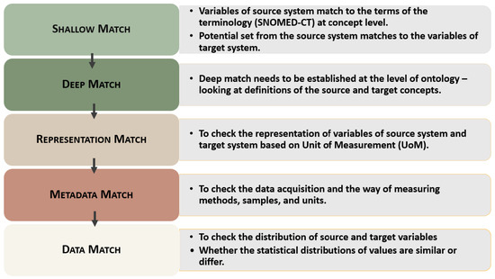
Figure 3.
Objective of each dimension with plausible differential scenarios.
Next, we evaluate the Metadata Match, which focuses on the method of data acquisition—something that cannot be assessed until the data are available in a numerical form. This sequence is important because each dimension is interdependent—the output of one stage becomes the input for the next. Therefore, all dimensions are sequentially and logically connected. Finally, once the data are numerically standardized, we conduct the Data Match to compare the variation and distribution of the data between the two systems.
6.1. Shallow Match
The main objective of the Shallow Match is to ensure the label matching of the input variables of the source system with respect to the terms of a terminology. In this context, we consider SNOMED-CT for its comprehensive coverage of the clinical domain.
As shown in Figure 4, this match involves two main steps. First, it verifies that the source system’s variables match the terms in the terminology at the concept level, ensuring that the source system and the terminology share a common syntactic understanding. In the second step, after obtaining the potential set of related terms from the source system’s terminology, these terms are matched to the available variables in the target system.
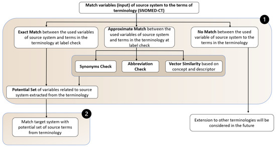
Figure 4.
Workflow of Shallow Match.
In the shallow match, there are three possible cases when matching input variables from the source system to the terminology: exact match, approximate match, and no match (which may require further extension towards a meta-thesaurus (other terminologies)).
- Exact Match: If the input variables of the source system exactly match the terms in the terminology, the resulting set from the source system is then matched with the variables in the target system.Example: The variable or input “Blood Pressure” from the source system is matched with the term of the terminology. Like “Blood Pressure as input” = “Blood Pressure in Terms of terminology”.
- Approximate Match: If there is no exact match, the input variables of the source system are checked using synonym lookup, abbreviation matching, and embedding-based similarity with respect to the terms in the terminology. The potential set is then matched with the variables in the target system.Example: If an exact match could not be found, but a similar term (terms) can be found in the terminology. For example, “BMI” in the source system has no direct match in the terminology. Then, in the case of an approximate match, it checks the abbreviations and synonyms of the terms and extracts the most relevant concepts as the resulting set.
- No Match: In the case of no match, there is a need to incorporate other terminologies or meta-thesaurus, which will be considered in future extensions.Example: Suppose we have two systems, each having a set of variables. The variables of the first system include diabetes diagnosis details, which are directly aligned with SNOMED-CT terms. However, the variables in the second system contain medication details for the diabetes condition that do not map to SNOMED-CT, even after applying a shallow match. In this case, direct matching of the two sets of variables using a single ontology/terminology is not possible, potentially requiring different ontologies/terminologies for matching.In practice, data dictionaries may be incomplete, and metadata and ontology mappings can vary significantly across healthcare providers. Some healthcare providers use a single terminology, whereas others operate in multi-terminology environments depending on the requirements of CDSS or related applications. Moreover, data dictionaries may be incomplete, variable definitions may be missing, and mappings between variables and ontology concepts may be ambiguous or missing. These challenges become more complex in multi-terminology environments, where multiple clinical vocabularies coexist and may represent the same concept differently across terminologies. For example, a clinical concept may have different definitions or hierarchical structures across terminologies such as SNOMED-CT, the Medical Dictionary for Regulatory Activities (MedDRA) [55], or the International Classification of Diseases (ICD) [56]. Such inconsistencies may lead to one-to-many mappings or semantic ambiguity when aligning variables across healthcare ecosystems. When the target ecosystem contains multiple terminologies, a unified metathesaurus can be used to map variables to SNOMED-CT concepts in the source ecosystem. Even in single-terminology settings, identifying variable differences remains challenging. The proposed framework does not provide a complete multi-terminology solution. Instead, the framework assumes a single terminology to support the conceptual and logical representation of variable differences between healthcare providers. In this work, the standardization or mapping process is treated as a pre-processing step within the Shallow Match dimension of the SMD framework. Once the “Used Variables” are standardized with respect to SNOMED-CT, the SMD framework is applied to identify and represent differences between the two healthcare providers across dimensions. This step establishes a consistent semantic reference and reduces ambiguity in variable definitions. If a direct mapping cannot be established using SNOMED-CT, an approximate matching strategy is applied, as discussed in the shallow match. If the automatic mapping with the single terminology fails or creates uncertainty, then it may be necessary to use more than one ontology, such as ICD, Logical Observation Identifiers Names and Codes (LOINC) [57], Unified Medical Language System (UMLS) [58], and Health Level 7 (HL7) [59]. In this research, we consider the first two scenarios of Shallow Match, namely exact and approximate matching, and we will later explore the integration of other terminologies.
In Shallow Match, the “Potential Set” of variables is selected from the terminology (for example, SNOMED-CT). Each input variable from the source system may yield multiple related terms from the terminology, even in cases of exact or approximate matches. These related terms form a pool of potential matches for comparison with the target system. To identify the most suitable variable from this potential set, the following scrutinizing approach is applied:
- 1.
- Score-Based Filtering: Select the top-ranking term based on similarity scoring, which may include string similarity and semantic embedding distance.
- 2.
- Presence Check in Target System: Validate whether the top-scoring candidate term has a corresponding representation in the target system’s variable set.
After applying the scrutinizing approach to narrow down the “Potential Set” from the source system, the process proceeds to step 2, where it matches the variables to those in the target system. There are two possible outcomes when matching the resulting set with the variables of the target system: matchable (existing in the target system) and missing variables (not existing in the target system). In the first scenario, once a match is found, it proceeds to the Deep Match. In the case of missing variables, it is necessary to identify a plausible surrogate.
6.2. Output of Shallow Match
- 1.
- Match: After performing the internal process of “Shallow Match”, if the variables are available in both data ecosystems, then it moves to “Deep Match” for checking the definition of the concept.
- 2.
- No Match: If there is no match, then it assumes a variable missing case. Further analysis will be performed to identify a suitable surrogate or other adaptation.
Table 1 depicts an example of the output of shallow match considering the source variable and target variable.

Table 1.
Example of output of Shallow Match.
6.3. Deep Match
After conducting the Shallow Match, it is necessary to check the definition of concepts between the source system and the target system because the Shallow Match is not only sufficient to establish the similarity of variables. In many cases, the same concept can have more than one definition. In other words, Deep Match is essential to check the definitions of the source and target concepts at the ontology level. Figure 5 depicts the workflow of the deep match.
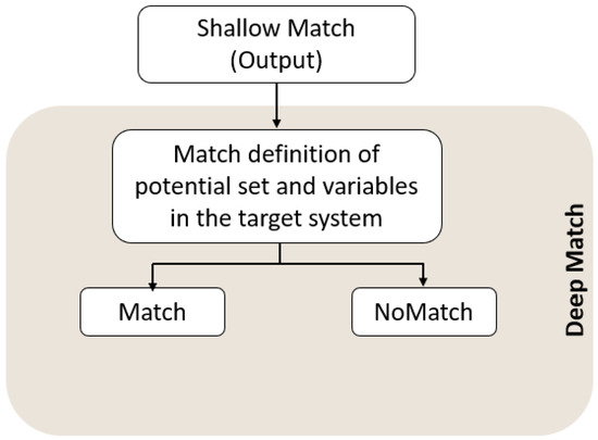
Figure 5.
Workflow of Deep Match.
Example: the source system defines “Blood Pressure” as “the pressure exerted by circulating blood upon the walls of blood vessels”, while the target system defines “Blood Pressure” as “the force of blood pushing against the walls of arteries.” In both terms, the definitions are the same.
6.4. Output of Deep Match
- 1.
- Match: Both systems define the variable in a semantically identical manner.
- 2.
- No Match: The variables of both systems have different meanings, leading to potential semantic conflict.Table 2 depicts an example of the output of deep match considering the source variable and target variable based on the definition.
Table 2. Examples of Deep Match outcomes based on definition comparison.
6.5. Representation Match
This dimension checks the data encoding and unit of measurement (UoM) of variables in both systems to determine whether there are any differences. Figure 6 depicts the possibilities of differences in representation.
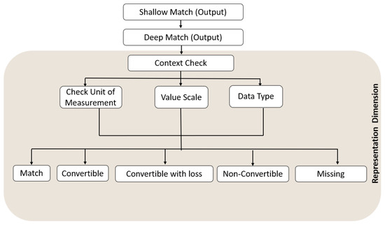
Figure 6.
Workflow of Representation Match.
After checking the differences between variables in the source and target systems in Deep Match, we proceed to Representation Match, where the first check is whether the data value is in numerical or contextual format. If both variables are numerically represented, then the differential checks proceed to the UoM. While the UoM is the same for both variables, it proceeds to Metadata Match.
To ensure transparency and reproducibility, a rule-based decision process maps variables between the source and target ecosystems based on representation attributes such as Unit of Measurement (UoM), data type, and value scale. The decision rules are mainly derived from two sources. First, it comes from medical background knowledge and clinical formulas, which enable deterministic transformations using LOINC, UCUM, and NPU for unit conversion; for example, mg/dL to mmol/L or derived variables; for example, BMI from height and weight. Secondly, rule-based knowledge is derived from reference metadata or clinical guidelines, such as laboratory reference ranges, to standardize categorical or numerical representations. First, the system checks whether the representation attributes of the source and target variables are identical. If they are the same, the variable can be directly reused for redeployment. If differences exist, the system checks whether a deterministic transformation rule exists that converts the attributes to a common unit or value scale. In some cases, transformations may be possible but may introduce loss of precision or information, and such representation differences are recorded accordingly. When no valid transformation rule exists between the attributes of the variables, manual mapping may be required. Finally, if attributes of any variable, such as UoM, data type, or scale, are missing, then the “Mutator” evaluates the situation and devises the fallback strategies of whether the variable should be mapped, reconstructed, or omitted from the redeployment process. Table 3 represents the decision rules for mapping quantitative measures to discrete representation output labels.
Table 3.
Decision rules for representation output labels.
Example: If the source system measures “Fasting Blood Glucose (FBG)” in milligrams per deciliter (mg / dL) and the target system measures in millimoles per liter (mmol/L). Therefore, it is necessary to convert the UoM to a common unit. In the range check, the source system represents the “Glucose Level” in the form of “0”, “1”, and “2”, and the target system shows it in the form of different ranges as normal (70–100 mg/dL), pre-diabetic (101–125 mg/dL), and diabetic (125+ mg/dL), respectively. Thus, the “Glucose level” ranges differ between the two systems. To standardize the ranges of both variables, the knowledge will be taken from the reference data or external pathological reports (MetaData) to categorize them into classes, such as 0 for normal, 1 for pre-diabetic, and 2 for diabetic, for both variables.
6.6. Output of Representation Match
- 1.
- Match: The variables in both systems are represented in the same format and unit.
- 2.
- Convertible: A transformation is possible without losing meaning or information (for example, unit conversion from mg/dL to mmol/L).
- 3.
- Convertible with Loss: The transformation results in reduced semantic precision (for example, mapping qualitative labels to numeric codes).
- 4.
- Non-Convertible: The formats are fundamentally incompatible and cannot be reconciled (for example, image format vs. numerical score).
- 5.
- Missing: The information of representation is missing in the target variable.
Table 4 depicts the examples of the output of representation match, considering the source variable and target variable based on the representation.
Table 4.
Examples of representation match outcomes.
6.7. MetaData Match
Figure 7 depicts the possibility of differences at MetaData Match, where the differences are identified in the ways of collecting the health data. The first differential check in the metadata match is how the health data are collected, including the measurement device, who measured the data, the sample type, and the instant at which the measurement was taken. Afterwards, it checks the interval to ensure the context of the collected data is consistent across both variables. This context must match for the CDSS to operate correctly in the target system.
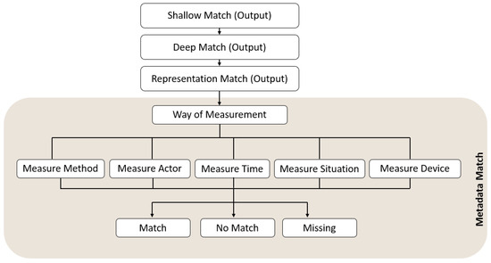
Figure 7.
Workflow of Metadata Match.
Example: The source system has a variable that shows the glucose level of a patient that was measured through a blood sample using an electronic device by the patient. In the target system, the pathologist measures urinary glucose levels. Therefore, changes in the sample mode or in the methods used to measure glucose will result in differences between the variables of the two systems.
6.8. Output of Metadata Match
- 1.
- Match: The metadata related to the way of data collection, measurement method, measurement situation, measure actor, and timing are identical.
- 2.
- No Match: Major inconsistencies exist in how the data were collected or defined, making standardization difficult without significant transformation.
- 3.
- Missing: Required metadata information (for example, device used or measurement protocol) is absent from one of the systems, requiring external inference or estimation.
Table 5 depicts an example of the output of metadata match considering the source variable and target variable.
Table 5.
Illustrative examples of Metadata match outcomes.
6.9. Data Match
Figure 8 depicts the possibility of differences based on the distribution of data values. In this match, the distributions of the two variables will be compared to determine whether they are similar or different. If the distributions of a variable are identical, the match case does not require further readjustment and can be reused directly in the redeployment process. Otherwise, statistical inference can be employed to analyze these differences based on the data types [60], such as Time Series, Discrete, Continuous, Mixed (Discrete + Continuous), Categorical, and Ordinal.
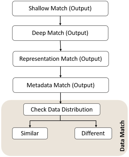
Figure 8.
Workflow of Data Match.
Example: the source system has a variable “HbA1c level”, and this level is measured in patients who are young, like 20–40 years old, with Type 1 diabetes. In this case, the range is between 6.5% and 7.5%, indicating a narrow distribution. On the flip side, if the target system has an HbA1c level measured in a patient aged over 50 years with type 2 diabetes, then the distribution range will be between 7% and 10%, so a wider distribution might be expected.
Output of Data Match
- 1.
- Similar: The data distribution between source and target systems for a given variable is statistically consistent and comparable. For example, both providers have nearly identical distributions for “Age” or “Glucose Level”.
- 2.
- Different: The distributions are significantly different in both central tendency and shape. This could include distributions, skewness, or outliers that are unique to a single provider. The “Different” category is further classified into three cases: “highshift”, “lowshift”, and “missing value”.
Table 6 depicts an example of the output of data match considering the source variable and target variable.
Table 6.
Examples of Data Match outcomes based on statistical distribution.
7. Conceptual Modeling of Variable Differences
Figure 9 depicts a conceptual model named “VarDiff” that provides a machine-interpretable, standardized, and formally structured representation of differences between the “Used Variables” and “Visible Variables” of two data ecosystems. The “red arrow” represents the starting point of this conceptual model. It encompasses variable descriptions and multidimensional match outcomes. Figure 10 illustrates aggregated differential states and adaptation scenario classifications along with their categories. Semantic representation helps describe and manage the variety in structure, contextual relationships, provenance, and access visibility, and organizes them into a structured form for machine interpretation [61]. Variable descriptions provide the foundational semantic characterization of each variable within the data ecosystems. It formally captures attributes, such as label, clinical definition, unit of measurement, data type, representation format, value scale, measurement method, distribution characteristics, reference ranges, and contextual usage. The match outcomes represent aggregated results derived from the Shallow, Deep, Representation, Metadata, and Data dimensions. Each dimension has a specific level of alignment, such as terminology equivalency, semantic consistency, format compatibility, contextual metadata alignment, and distributional similarity. These outcomes for each dimension include differences in the form of logical states (e.g., Match, NoMatch, Missing, Convertible, Non-Convertible, Convertible With Loss, Similar, and Different), thereby enabling machine-interpretable reasoning. The identified match outcomes for each dimension are aggregated into adaptation categories, such as “Direct Reuse”, “Transformative”, “Reconstructive”, and “Incompatible”. These categories operationalize the reasoning process in “Mutator” to deterministically devise actionable strategies.
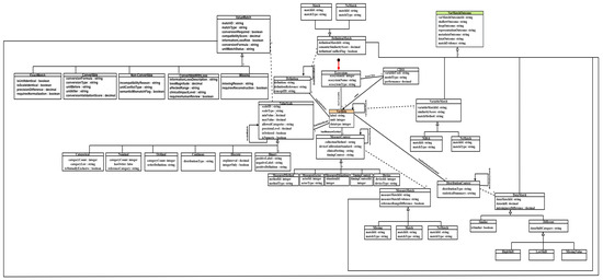
Figure 9.
A conceptual model of outcomes of differences based on the used variable and visible variables across healthcare ecosystems (Part A).
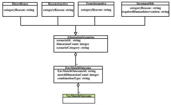
Figure 10.
A conceptual model to generate the match outcomes combinations and categories (Part B).
This conceptual model represents the concepts, data objects, data properties, and reasoning flow included within the “VarDiff”. There exist two ecosystems named “Source Ecosystem” and “Target Ecosystem” within the concept “Ecosystem”, where a Bayesian network-based CDSS is hosted on the “Source System” within the concept “CDSS”. The variable used in “SourceCDSS” is known as “Used Variables”, and the available variables in the “Target Ecosystem” are known as “Visible Variables”. This conceptual model provides a structured representation to systematically capture the output of differences between the variables of two ecosystems. The concept “Variable” is linked with the concept “Ecosystem” through hasVariable and includes properties of “used variable” and “visible variable”, such as “label”, “unit”, and “datatype”. It is further linked to ValueScale, MeasureContext, Definition, and DistributionContext through hasValueScale, hasMeasureContext, hasDefinition, and hasDistributionContext, respectively. These four explicit concepts further characterize the properties of “Used Variable” and “Visible Variable”: the scale information for the representation dimension, the data acquisition for the metadata dimension, the definition reference for the deep dimension, and the statistical summary for the data dimension. The “Variable” concept also captures label-level matching information for the shallow dimension. In addition, the match results of “ValueScale”, “MeasureContext”, “Definition”, “Variable”, and “DistributionContext” are aggregated in the concept “VarMatchOutcome”. Each interlinked concept to “Variable and itself contains a recursive loop that represents the one-by-one comparison of “Used Variable” and “Visible Variables”. The concept of “Variable” and its explicit concepts, such as ValueScale, MeasureContext, Definition, and DistributionContext, have the matching results. The concept “VarMatchOutcome” aggregates matching results across the five dimensions, such as “ShallowMatch”, “DeepMatch”, “RepresentationMatch”, “MetadataMatch” and “DataMatch”. The possible match outcomes are then aggregated into “EnvMatchOutcome”. The reasoning proceeds hierarchically: label matching evaluates variable availability by comparing the “Used Variables” with the “Visible Variables”, the value-scale compatibility is evaluated to detect structural incompatibility; measurement context and semantic equivalence are then examined to ensure clinical meaning preservation; finally, statistical similarity is assessed to detect distributional shifts. Based on the aggregated match outcomes from all five dimensions, the concept “AdaptationScenarios” is inferred to classify the adaptation scenarios into the four adaptation categories, such as “Direct Reuse”, “Transformative”, “Reconstructive”, or “Incompatible”. In the concept “Direct Reuse”, the variables of both ecosystems are matchable across structural, semantic, contextual, and statistical dimensions. Therefore, no transformation is required, and they may be reused directly for the redeployment of a CDSS. In the concept “Transformative”, the variables of both ecosystems are matchable at label and definition, but there is a need to apply the controlled transformation due to contextual differences at representation dimension and data dimension, such as datatype conversion, unit normalization, or distribution alignment. In the concept “Reconstructive”, when the required variable is missing or structurally unusable in the target ecosystem, then there is a need to find the relevant surrogate for the redeployment. Lastly, in the concept “Incompatible”, incompatibilities exist at the semantic, structural, or statistical level and cannot be resolved. These outcomes determine whether the variable can be reused directly, requires transformation, must be reconstructed via surrogate modeling, or should be excluded. The “Mutator” module then supports transformation and surrogate handling by generating adaptation strategies and execution plans to enable CDSS redeployment, thereby supporting more efficient and structured CDSS adaptation.
8. Decision Matrix of Possible Match Outcomes
Table 7 depicts the decision matrix of differential outcomes based on the “VarDiff” to show all logically possible combinations of match results obtained across the five differential dimensions, where “M” stands for “Match”, “NM” stands for “NoMatch”, “S” represents for “Surrogate”, “NonConv” stands for “NonConvertible”, “Conv” stands for “Convertible”, and “ConvLoss” stands for “ConvertibleWithLoss”. The nineteen adaptation scenarios are systematically derived by logically combining dimensional match outcomes, ensuring an exhaustive and deterministic mapping of differential combinations to their corresponding adaptation strategies within the “Mutator” component. All these possible match results are aggregated under the class “EnvMatchOutcome”, and the aggregated results are classified into four differential categories in “AdaptationScenarios” as given below:
Table 7.
Decision matrix of differential outcomes from each dimension.
From “VarDiff”, the differential reasoning yields nineteen logical combinations depending on the nature of the dimension outcomes. In each scenario of “NM”, “NonCov”, and “Missing”, there exist two possibilities: one is with a surrogate, and the other is without a surrogate. Within the decision matrix, one trivial scenario occurs when all dimensional outcomes are classified as Match. In this case, no adaptation is required, and the scenario is categorized under “Direct Reuse”. Seven adaptation scenarios fall under the “Reconstructive” category, where surrogate identification is necessary to compensate for missing or non-matching variables. Another eight scenarios correspond to the “Incompatible” category, in which human intervention or an alternative adaptation strategy—potentially devised by the mutator—is required due to substantial semantic or structural divergence. The remaining three scenarios are classified as “Transformative”, where automatic conversion or reconciliation is feasible based on planner guidance derived from the “Mutator” component. Additionally, certain adaptation scenarios require the resolution of specific dimensional outcomes before evaluating subsequent dimensions. In some cases, subsequent conditions are not applicable because the decision has already been determined by the early-dimension condition, and these conditions are represented by “–” in the decision matrix. All nineteen adaptation scenarios are processed by the “Mutator” component, which generates appropriate adaptation strategies to enable the necessary readjustment.
To better understand the adaptation categories, we have provided examples for each. In the “Direct Reuse”, the source and target variables have identical definitions, representations, metadata context, and statistical distributions; this condition ensures that the particular variable to be reused directly; for example, a “blood pressure” recorded with the same meaning, representation, measurement characteristics, and data distributions in both healthcare providers. In the “Transformative” category, the variables are semantically consistent but require controlled transformations due to representation differences, such as when “glucose” values are recorded in different units; for example, mg/dL versus mmol/L, and require unit conversion. However, a transformation may be possible when the shift in the data distribution is small. The “Reconstructive” scenario occurs when a required variable is missing in the target ecosystem but can be reconstructed using other available variables as a surrogate; for instance, if Body Mass Index (BMI) is not directly available but can be derived from height and weight. Finally, the “Incompatible” represents conditions where the differential outcomes are “NM”, “NonConv”, “Missing”, and “HighShift”; for example, when a source variable is represented as an imaging-based score while the target ecosystem contains textual clinical notes.
9. Identification of Mutation Strategies
Once the SMD framework is established to describe the internal workings of the “Differentiator” and its differential workflows for each dimension, such as Shallow, Deep, Representation, Metadata, and Data, these workflows are formally defined using “VarDiff”. This conceptual model comprises the foundational reasoning structure of the framework for representing how to capture differences between variables across these dimensions and their resulting adaptation scenarios and categories. Subsequently, the identified adaptation categories are processed by the “Mutator” component, which analyzes adaptation scenarios and supports the selection of appropriate adaptation strategies for CDSS readjustment.
The “Mutator” component of ASF generates candidate CDSSs based on adaptation rules after identifying differential situations across the five dimensions. The Mutator’s core process involves identifying the adaptation type, devising adaptation strategies, and selecting the best set of candidates. The “Mutator” is an iterative process that incrementally discovers relevant and available variables within the healthcare provider (target) to construct feasible adaptation strategies. In addition, the “Mutator” supports the derivation of appropriate adaptation strategies for the identified adaptation types and their corresponding differential situations.
The iterative nature of the “Mutator” enables continuous refinement: when differences are detected at any dimension, alternative adaptation strategies can be explored across other dimensions. The “Mutator” reconciles these differences by systematically selecting the most suitable strategy. For example, within the Representation Match dimension, if a variable is identified as non-convertible, the “Mutator” may backtrack to the Shallow Match and Deep Match dimensions to search for clinically and semantically equivalent surrogate variables that can replace the non-convertible variable in the target healthcare provider. Here, we describe the role and significance of the “Mutator” in the redeployment process after categorizing match outcomes into four categories: “Direct Reuse”, “Transformative”, “Reconstructive”, and “Incompatible”. A detailed description of the “Mutator” and its adaptation strategies is considered future work.
Figure 11 depicts the flow of transferring the possible matches from each dimension into the “Mutator”. Each dimension having possible matches such as (M, NM), (M, NM), (M, Conv, ConvLoss, NonConv, Missing), (M, NM, Missing), and (Similar, Different) from the Shallow Match, Deep Match, Representation Match, Metadata Match, and Data Match, respectively, are aggregated and generate the possible combination of outcomes in the form of a decision matrix. The decision matrix comprises four categories, defined by the exhaustive combination of outcomes. According to the identified scenarios and categories, “Mutator” will generate the adaptation type that determines which knowledge (medical, data science, or hybrid) is most applicable for devising the adaptation strategies. Here, the required adaptation strategies are applied according to the categories to generate candidate Bayesian CDSSs. Among these, the best candidate will be chosen for redeployment based on validation (both qualitative and quantitative).
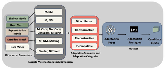
Figure 11.
Difference-driven classification and adaptation process.
The “Mutator” helps automatically construct plans for how the “Used Variable” of the source CDSS can be matched with the “Visible Variables” in the target healthcare providers. If the variable is directly available between both source and target healthcare providers, then it can be used without any change. Otherwise, the “Mutator” checks whether it can be transformed or reconstructed from available variables. This follows a recursive process to determine which variables are available and whether they can be transformed when differences exist among them and to derive the process for obtaining the set of preferred plans. To select the best transformation strategies, the planner evaluates them using preference metrics or error metrics. Finally, the most promising transformation plans are evaluated on validation datasets from the target healthcare provider, enabling the system to select the most suitable strategy for CDSS redeployment across healthcare providers. For example, in the “Reconstructive” category, there are one or more variables of the source ecosystem that may be missing in the visible variables of the target ecosystem. The “Mutator” will be responsible for identifying surrogate variables from the visible variables in the target ecosystem through logical relationships, statistical inference, or domain knowledge rules. Depending on the number and nature of missing variables, the “Mutator” triggers different planning strategies, such as “SingleMissingSingleSurrogatePlan”, “SingleMissingMultipleSurrogatesPlan”, “MultipleMissingIndependentSurrogatesPlan”, or “MultipleMissingMultipleSurrogatePlan”, which represent different reconstruction scenarios based on whether one or multiple variables are missing for redeployment of a CDSS.
10. Case Study
In this case study, a CDSS for predicting the risk of cardiovascular disease (CVD) operates in a source system using input variables (“used variables”) such as sex (female/male), age (years), weight (kg), height (m), BMI, abdominal circumference (m), blood pressure (mmHg), total cholesterol (mg/dL), HDL (mg/dL), fasting blood sugar (mg/dL), smoking (Y/N), and CVD risk (target node). To redeploy the existing CDSS from the source system to a target system with available variables such as sex (1/2), age (days), weight (kg), height (cm), systolic blood pressure (hg), diastolic blood pressure (hg), cholesterol (1–3 scale), alcohol intake (1/2), physical activity (0/1), glucose (1–3 scale), smoking (0/1), and cardiovascular disease (target node). The variables in the source and target ecosystems are derived from two datasets corresponding to the same CVD use case, where one dataset is treated as the https://data.mendeley.com/datasets/vhgyn5yk4g/1 “source system” (accessed on 22 March 2026) and the other as the https://github.com/ShilpaAjitheks/Cardiovascular-disease-prediction/tree/master?tab=readme-ov-file#source-of-the-dataset-used “target system” (accessed on 22 March 2026). Therefore, it is necessary to identify the different situations in which variables differ across the five differential dimensions.
As illustrated in Figure 12, this mismatch necessitates a structured assessment of how each variable of the source system aligns with the variables of the target system. To address redeployment challenges and support systematic analysis, we categorize differential situations by dimension to systematically determine the adaptation requirements for each variable. Each scenario requires domain knowledge, data science expertise, or a combination of both to devise appropriate adaptation strategies.
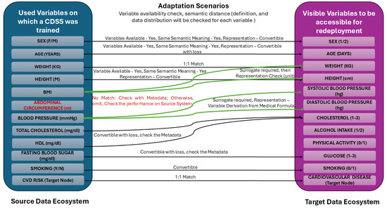
Figure 12.
Cardio vascular disease (CVD) data mapping.
The variable Sex is available in both systems and shares the same semantic meaning; however, its representation differs (female/male in the source system versus 1/2 in the target system). This difference is directly convertible, requiring a simple categorical transformation. Similarly, Age is available in both systems but is reported in years in the source system and in days in the target system. Although this conversion is feasible, it may introduce precision differences, requiring careful handling to avoid unintended information loss. “Lossy conversion” refers to situations in which a transformation between variables is possible but may introduce small inaccuracies or loss of precision that could affect the performance of the redeployed CDSS.
The variable Weight is available in both systems with identical units and semantics, and therefore requires no adaptation. This is a trivial case in which the variable maps one-to-one between the two systems. The variable Height is represented in meters in the source system and centimeters in the target system. It requires only a unit conversion, after which metadata alignment is evaluated.
More complex scenarios arise when variables are missing or structurally incompatible. For instance, Body Mass Index (BMI) is not explicitly available in the target system but can be derived as a surrogate variable using height and weight, provided that unit consistency, metadata alignment, and clinical validity are ensured. Conversely, Abdominal Circumference is unavailable in the target system and lacks a clinically justified surrogate. In this case, the variable is omitted, and its impact on CDSS performance is evaluated relative to the source system using ablation or sensitivity analysis. In some cases, when a variable is clinically important and cannot be omitted, and its omission may significantly affect the CDSS’s sensitivity, manual intervention becomes necessary.
Blood Pressure variables present a non-trivial adaptation scenario, in which the source system contains a Blood Pressure (mmHg) variable, whereas the target system contains Systolic and Diastolic Blood Pressure. This situation requires medical knowledge-based adaptation strategies to determine whether and how these variables can be used directly, or whether they require recombination via clinically validated formulas.
Laboratory variables such as Total Cholesterol, HDL, and Fasting Blood Sugar are available in the target system only as ordinal scales (1–3) rather than continuous measurements. These cases are classified as convertible with information loss, requiring metadata validation and data-driven sensitivity analysis. Similarly, lifestyle variables such as Smoking, Alcohol Intake, and Physical Activity demonstrate representation differences but are largely convertible, provided that category semantics and clinical interpretations are preserved.
Once differential outputs are obtained across five dimensions for each variable, then the combination of outputs is classified into four adaptation categories to determine the appropriate adaptation strategy. For example, the variable Weight, which has the same semantic meaning, representation, metadata, and data distribution across both healthcare providers, typically falls under the Direct Reuse category, meaning that no further adaptation is required. Variables such as Sex and Height, which exhibit representation differences but can be transformed using deterministic rules, such as categorical encoding and unit conversion, respectively, are classified as Transformative. In cases where a variable is missing in the target system but can be derived using available variables, such as BMI reconstructed from Height and Weight, the situation falls under the Reconstructive category, requiring surrogate variable identification and validation. On the other hand, when variables are absent and no clinically valid surrogate exists, such as Abdominal Circumference, the variable is classified as Incompatible or Reconstructive, depending on the absence or presence of a valid surrogate, respectively, and its impact on the CDSS is evaluated through model sensitivity. Similarly, variables represented as ordinal categories rather than continuous measurements, such as Cholesterol and Glucose, fall under the Transformative category, potentially incurring information loss, and require additional metadata and statistical assessment. Finally, the variable CVD is considered in the Transformative category. These adaptation categories enable the framework to translate variable-level differences into structured adaptation strategies, thereby supporting systematic analysis and informed adaptation of CDSS across heterogeneous healthcare providers. Table 8 presents the variable-level outputs across all five dimensions and corresponding adaptation categories, as derived from the decision matrix, to provide clarity for the presented case study.
Table 8.
Variable-level outputs across five differential dimensions.
11. Conclusions and Future Work
CDSS redeployment across healthcare providers involves two key steps: identifying variable-level differences and devising readjustment plans to redeploy an existing CDSS to a new healthcare provider. CDSS redeployment can reduce manual effort, cost, and development time while improving code reusability and maintaining CDSS standards.
The main contribution of this paper is the identification of five differential dimensions, such as shallow, deep, representation, metadata, and data, and their corresponding outputs for systematically analyzing variable-level differences across healthcare providers. We also propose a conceptual model, “VarDiff”, that provides a structured and logical representation of differential outcomes across dimensions, along with the characteristics of “used variables” and “visible variables”. This representation defines adaptation categories—Direct Reuse, Transformative, Reconstructive, and Incompatible—using a decision matrix to support adaptation reasoning within the “Mutator” component.
We present the SMD framework to identify the differential dimensions between the “used variables” and “visible variables”, their differential possibilities, and workflow executions across each dimension. The proposed framework is a single terminology-based solution to observe the variable differences across the five dimensions. Healthcare providers typically have fragmented data and different variables, which pose substantial barriers to redeployment and can make it costly to rebuild a CDSS for each provider. The SMD framework explicitly addresses these issues by decomposing them into manageable dimensions and categorizing all possible differences between the variables of both data ecosystems. This framework enables healthcare providers to reuse existing CDSSs rather than build new ones, thereby saving time and resources. Hence, for the redeployment of the CDSS, it is important to understand the underlying differential situations in each dimension. So accordingly, the adaptation type can be identified as requiring domain knowledge, data science knowledge, or a hybrid for adjusting the existing CDSS to a new environment.
In addition, the conceptual model “VarDiff” provides a formal representation of differences between variables across healthcare providers. It enables variable characteristics and cross-ecosystem differences to be encoded as logical states, supporting systematic mapping of dimension-level outcomes to adaptation categories. These outcomes are classified into four categories and provided as inputs to the “Mutator”. Future work will focus on extending the “Mutator” component to support adaptation strategy generation and evaluation.
Author Contributions
Conceptualization, G.G. (Gourav Gupta), J.S. and W.M.; methodology, G.G. (Gourav Gupta) and W.M.; investigation, G.G. (Gourav Gupta), W.M., J.S. and G.G. (Georg Grossmann); data curation, G.G. (Gourav Gupta); writing—original draft preparation, G.G. (Gourav Gupta); writing—review and editing, W.M., G.G. (Gourav Gupta), J.S. and M.S.; supervision, W.M., J.S., G.G. (Gourav Gupta) and M.S. All authors have read and agreed to the published version of the manuscript.
Funding
This research received no external funding.
Institutional Review Board Statement
Not applicable.
Informed Consent Statement
Not applicable.
Data Availability Statement
All data used in this study are publicly available.
Acknowledgments
This work is part of the Digital Health Cooperative Research Centre project ‘PreHaRM: A Predictive Harm Response Management algorithmic tool to reduce adverse events in healthcare settings’ (DHCRC-0156).
Conflicts of Interest
The authors declare no conflicts of interest.
References
- Gupta, G.; Stanek, J.; Mayer, W.; Grossmann, G. Adaptive Semantic Framework for CDSS to a new environment. In Proceedings of the 2024 Australasian Computer Science Week, Sydney, NSW, Australia, 29 January–2 February 2024; pp. 75–77. [Google Scholar]
- Almadani, B.; Kaisar, H.; Thoker, I.R.; Aliyu, F. A systematic survey of distributed decision support systems in healthcare. Systems 2025, 13, 157. [Google Scholar] [CrossRef]
- Greenes, R.A.; Bates, D.W.; Kawamoto, K.; Middleton, B.; Osheroff, J.; Shahar, Y. Clinical decision support models and frameworks: Seeking to address research issues underlying implementation successes and failures. J. Biomed. Inform. 2018, 78, 134–143. [Google Scholar] [CrossRef]
- Sutton, R.T.; Pincock, D.; Baumgart, D.C.; Sadowski, D.C.; Fedorak, R.N.; Kroeker, K.I. An overview of clinical decision support systems: Benefits, risks, and strategies for success. NPJ Digit. Med. 2020, 3, 17. [Google Scholar] [CrossRef]
- Ahmed, M.I.; Spooner, B.; Isherwood, J.; Lane, M.; Orrock, E.; Dennison, A. A systematic review of the barriers to the implementation of artificial intelligence in healthcare. Cureus 2023, 15, e46454. [Google Scholar] [CrossRef]
- Esmaeilzadeh, P. Challenges and strategies for wide-scale artificial intelligence (AI) deployment in healthcare practices: A perspective for healthcare organizations. Artif. Intell. Med. 2024, 151, 102861. [Google Scholar] [CrossRef]
- Weber, G.M.; Mandl, K.D.; Kohane, I.S. Finding the missing link for big biomedical data. Jama 2014, 311, 2479–2480. [Google Scholar] [CrossRef]
- Xiong, Z.; Wang, X.; Zhou, Y.; Keane, P.A.; Tham, Y.C.; Wang, Y.X.; Wong, T.Y. How Generalizable Are Foundation Models When Applied to Different Demographic Groups and Settings? NEJM AI 2025, 2, AIcs2400497. [Google Scholar] [CrossRef]
- Donovan, T.; Abell, B.; Fernando, M.; McPhail, S.M.; Carter, H.E. Implementation costs of hospital-based computerised decision support systems: A systematic review. Implement. Sci. 2023, 18, 7. [Google Scholar] [CrossRef] [PubMed]
- Pinsky, M.R.; Dubrawski, A.; Clermont, G. Intelligent clinical decision support. Sensors 2022, 22, 1408. [Google Scholar] [CrossRef] [PubMed]
- Yesankar, P.; Puri, C.; Gote, P.M. AI-Powered Clinical Decision Support Systems (CDSS): Challenges, Benefits, Applications, and Future Directions. In Proceedings of the 2025 International Conference on Machine Learning and Autonomous Systems (ICMLAS), Prawet, Thailand, 10–12 March 2025; IEEE: New York, NY, USA, 2025; pp. 1192–1197. [Google Scholar]
- Liang, W.; Tadesse, G.; Ho, D.; Fei-Fei, L.; Zaharia, M.; Zhang, C.; Zou, J. Advances, challenges and opportunities in creating data for trustworthy AI. Nat. Mach. Intell. 2022, 4, 669–677. [Google Scholar] [CrossRef]
- Mathew, A.S.; Salim, A. From Exorbitant to Affordable: The Evolution of AI Training Costs. Int. J. Emerg. Res. Areas (IJERA) 2025, 3, 112. [Google Scholar]
- Fan, D.P.; Ji, G.P.; Cheng, M.M.; Shao, L. Concealed object detection. IEEE Trans. Pattern Anal. Mach. Intell. 2021, 44, 6024–6042. [Google Scholar] [CrossRef]
- Guarino, N. Formal ontology, conceptual analysis and knowledge representation. Int. J. -Hum. -Comput. Stud. 1995, 43, 625–640. [Google Scholar] [CrossRef]
- Garbacz, P.; Kulicki, P.; Trypuz, R. A formal ontology of knowing and knowledge. Knowl. Manag. Res. Pract. 2012, 10, 206–226. [Google Scholar] [CrossRef]
- Das, S.; Hussey, P. Contsonto: A formal ontology for continuity of care. In pHealth 2021; IOS Press: Amsterdam, The Netherlands, 2021; pp. 82–87. [Google Scholar]
- Parsanasab, E.; Ahmadipour, A.; Mehraeen, E. Utilization of Ontology to Develop Artificial Intelligence Systems in the Healthcare Industry. Healthc. Inform. Res. 2025, 31, 320–330. [Google Scholar] [CrossRef]
- Schulz, S.; Stenzhorn, H.; Boeker, M.; Smith, B. Strengths and limitations of formal ontologies in the biomedical domain. Rev. Electron. De Comun. Inf. Inov. Em Saude RECIIS 2009, 3, 31. [Google Scholar] [CrossRef][Green Version]
- Kitson, N.K.; Constantinou, A.C.; Guo, Z.; Liu, Y.; Chobtham, K. A survey of Bayesian Network structure learning. Artif. Intell. Rev. 2023, 56, 8721–8814. [Google Scholar] [CrossRef]
- Wang, Q.A.; Lu, A.W.; Ni, Y.Q.; Wang, J.F.; Ma, Z.G. Bayesian network in structural health monitoring: Theoretical background and applications review. Sensors 2025, 25, 3577. [Google Scholar] [CrossRef] [PubMed]
- El-Sappagh, S.; Franda, F.; Ali, F.; Kwak, K.S. SNOMED CT standard ontology based on the ontology for general medical science. BMC Med. Inform. Decis. Mak. 2018, 18, 76. [Google Scholar] [CrossRef]
- Zeshan, F.; Mohamad, R. Medical ontology in the dynamic healthcare environment. Procedia Comput. Sci. 2012, 10, 340–348. [Google Scholar] [CrossRef]
- Norori, N.; Hu, Q.; Aellen, F.M.; Faraci, F.D.; Tzovara, A. Addressing bias in big data and AI for health care: A call for open science. Patterns 2021, 2, 100347. [Google Scholar] [CrossRef]
- Liyanage, H.; Krause, P.; De Lusignan, S. Using ontologies to improve semantic interoperability in health data. BMJ Health Care Inform. 2015, 22, 309–315. [Google Scholar] [CrossRef]
- del Carmen Legaz-García, M.; Martínez-Costa, C.; Menárguez-Tortosa, M.; Fernández-Breis, J.T. A semantic web based framework for the interoperability and exploitation of clinical models and EHR data. Knowl.-Based Syst. 2016, 105, 175–189. [Google Scholar] [CrossRef]
- Ambalavanan, R.; Snead, R.S.; Marczika, J.; Towett, G.; Malioukis, A.; Mbogori-Kairichi, M. Ontologies as the semantic bridge between artificial intelligence and healthcare. Front. Digit. Health 2025, 7, 1668385. [Google Scholar] [CrossRef]
- Tao, S.; Zeng, N.; Hands, I.; Hurt-Mueller, J.; Durbin, E.B.; Cui, L.; Zhang, G.Q. Web-based interactive mapping from data dictionaries to ontologies, with an application to cancer registry. BMC Med. Inform. Decis. Mak. 2020, 20, 271. [Google Scholar] [CrossRef] [PubMed]
- Burse, R.; Bertolotto, M.; O’Sullivan, D.; McArdle, G. Semantic interoperability: The future of healthcare. In Web Semantics; Elsevier: Amsterdam, The Netherlands, 2021; pp. 31–53. [Google Scholar]
- Koutras, C.; Siachamis, G.; Ionescu, A.; Psarakis, K.; Brons, J.; Fragkoulis, M.; Lofi, C.; Bonifati, A.; Katsifodimos, A. Valentine: Evaluating matching techniques for dataset discovery. In Proceedings of the 2021 IEEE 37th International Conference on Data Engineering (ICDE), Chania, Greece, 19–22 April 2021; IEEE: New York, NY, USA, 2021; pp. 468–479. [Google Scholar]
- Stroganov, O.; Fedarovich, A.; Wong, E.; Skovpen, Y.; Pakhomova, E.; Grishagin, I.; Fedarovich, D.; Khasanova, T.; Merberg, D.; Szalma, S.; et al. Mapping of UK Biobank clinical codes: Challenges and possible solutions. PLoS ONE 2022, 17, e0275816. [Google Scholar] [CrossRef]
- Matentzoglu, N.; Balhoff, J.P.; Bello, S.M.; Bizon, C.; Brush, M.; Callahan, T.J.; Chute, C.G.; Duncan, W.D.; Evelo, C.T.; Gabriel, D.; et al. A simple standard for sharing ontological mappings (SSSOM). Database 2022, 2022, baac035. [Google Scholar] [CrossRef]
- De Mello, B.H.; Rigo, S.J.; Da Costa, C.A.; da Rosa Righi, R.; Donida, B.; Bez, M.R.; Schunke, L.C. Semantic interoperability in health records standards: A systematic literature review. Health Technol. 2022, 12, 255–272. [Google Scholar] [CrossRef]
- Zare, M.; Pahl, C.; Nilashi, M.; Salim, N.; Ibrahim, O. A review of semantic similarity measures in biomedical domain using SNOMED-CT. J. Soft Comput. Decis. Support Syst. 2015, 2, 1. [Google Scholar]
- Clunis, J. Enhancing health-care data integration via automated semantic mapping. Electron. Libr. 2023, 41, 801–816. [Google Scholar] [CrossRef]
- Luschi, A.; Petraccone, C.; Fico, G.; Pecchia, L.; Iadanza, E. Semantic ontologies for complex healthcare structures: A scoping review. IEEE Access 2023, 11, 19228–19246. [Google Scholar] [CrossRef]
- Calcagno, S.; Calvagna, A.; Tramontana, E.; Verga, G. Merging Ontologies and Data from Electronic Health Records. Future Internet 2024, 16, 62. [Google Scholar] [CrossRef]
- Zahra, F.A.; Kate, R.J. Obtaining clinical term embeddings from SNOMED CT ontology. J. Biomed. Inform. 2024, 149, 104560. [Google Scholar] [CrossRef] [PubMed]
- Bietenbeck, A.; Streichert, T. Preparing laboratories for interconnected health care. Diagnostics 2021, 11, 1487. [Google Scholar] [CrossRef] [PubMed]
- Joint Committee on Nomenclature, Properties and Units (C-SC-NPU) of the IFCC and IUPAC; Pontet, F.; Petersen, U.M.; Fuentes-Arderiu, X.; Nordin, G.; Bruunshuus, I.; Ihalainen, J.; Karlsson, D.; Forsum, U.; Dybkaer, R.; et al. Clinical laboratory sciences data transmission: The NPU coding system. Stud. Health Technol. Inform. 2009, 150, 265. [Google Scholar] [PubMed]
- Vogl, K.; Ingenerf, J.; Kramer, J.; Chantraine, C.; Drenkhahn, C. LUMA: A mapping assistant for standardizing the units of LOINC-coded laboratory tests. Appl. Sci. 2022, 12, 5848. [Google Scholar] [CrossRef]
- Monjas, A.M.; Ruiz, D.R.; Del Rey, D.P.; Palchuk, M.B. Enhancing real world data interoperability in healthcare: A methodological approach to laboratory unit harmonization. Int. J. Med. Inform. 2025, 193, 105665. [Google Scholar] [CrossRef]
- Maillet, N.; Collet, G.; Vannier, T.; Lavenier, D.; Peterlongo, P. COMMET: Comparing and combining multiple metagenomic datasets. In Proceedings of the 2014 IEEE International Conference on Bioinformatics and Biomedicine (BIBM), Belfast, UK, 2–5 November 2014; IEEE: New York, NY, USA, 2014; pp. 94–98. [Google Scholar]
- Raff, P.; Jin, Z. The difference-of-datasets framework: A statistical method to discover insight. In Proceedings of the 2016 IEEE International Conference on Big Data (Big Data), Washington, DC, USA, 5–8 December 2016; IEEE: New York, NY, USA, 2016; pp. 1824–1831. [Google Scholar]
- Chang, E.; Mostafa, J. The use of SNOMED CT, 2013–2020: A literature review. J. Am. Med. Inform. Assoc. 2021, 28, 2017–2026. [Google Scholar] [CrossRef]
- Tikkinen, K.A.; Halme, A.L.; Guyatt, G.H.; Glasziou, P. The Impact of Definitions of Disease on Overdiagnosis. JAMA Intern. Med. 2025, 185, 909–910. [Google Scholar] [CrossRef]
- Riveros, C.; Jan, N.V.S.; Vrgoč, D. Rematch: A novel regex engine for finding all matches. Proc. VLDB Endow. 2024, 16, 2792–2804. [Google Scholar] [CrossRef]
- Berger, B.; Waterman, M.S.; Yu, Y.W. Levenshtein distance, sequence comparison and biological database search. IEEE Trans. Inf. Theory 2020, 67, 3287–3294. [Google Scholar] [CrossRef] [PubMed]
- Majumder, G.; Pakray, P.; Gelbukh, A.; Pinto, D. Semantic textual similarity methods, tools, and applications: A survey. Comput. Y Sist. 2016, 20, 647–665. [Google Scholar] [CrossRef]
- Alsentzer, E.; Murphy, J.R.; Boag, W.; Weng, W.H.; Jin, D.; Naumann, T.; McDermott, M. Publicly available clinical BERT embeddings. arXiv 2019, arXiv:1904.03323. [Google Scholar] [CrossRef]
- Soriano, I.M.; Peña, J.L.C.; Breis, J.T.F.; San Román, I.; Barriuso, A.A.; Baraza, D.G. Snomed2Vec: Representation of SNOMED CT terms with Word2Vec. In Proceedings of the 2019 IEEE 32nd International Symposium on Computer-Based Medical Systems (CBMS), Cordoba, Spain, 5–7 June 2019; IEEE: New York, NY, USA, 2019; pp. 678–683. [Google Scholar]
- Chen, Z.; Cano, A.H.; Romanou, A.; Bonnet, A.; Matoba, K.; Salvi, F.; Pagliardini, M.; Fan, S.; Köpf, A.; Mohtashami, A.; et al. Meditron-70b: Scaling medical pretraining for large language models. arXiv 2023, arXiv:2311.16079. [Google Scholar] [CrossRef]
- Chang, E.; Sung, S. Use of SNOMED CT in Large Language Models: Scoping Review. JMIR Med. Inform. 2024, 12, e62924. [Google Scholar] [CrossRef]
- Singhal, K.; Azizi, S.; Tu, T.; Mahdavi, S.S.; Wei, J.; Chung, H.W.; Scales, N.; Tanwani, A.; Cole-Lewis, H.; Pfohl, S.; et al. Large language models encode clinical knowledge. arXiv 2022, arXiv:2212.13138. [Google Scholar] [CrossRef]
- Brown, E.G.; Wood, L.; Wood, S. The medical dictionary for regulatory activities (MedDRA). Drug Saf. 1999, 20, 109–117. [Google Scholar] [CrossRef] [PubMed]
- World Health Organization. International Classification of Diseases-ICD; World Health Organization: Geneva, Switzerland, 2009. [Google Scholar]
- Forrey, A.W.; Mcdonald, C.J.; DeMoor, G.; Huff, S.M.; Leavelle, D.; Leland, D.; Fiers, T.; Charles, L.; Griffin, B.; Stalling, F.; et al. Logical observation identifier names and codes (LOINC) database: A public use set of codes and names for electronic reporting of clinical laboratory test results. Clin. Chem. 1996, 42, 81–90. [Google Scholar] [CrossRef]
- Elkin, P.L.; Brown, S.H. Unified medical language system (UMLS). In Terminology, Ontology and Their Implementations; Springer: Berlin/Heidelberg, Germany, 2023; pp. 463–474. [Google Scholar]
- Joyia, G.J.; Akram, M.U.; Akbar, C.N.; Maqsood, M.F. Evolution of health level-7: A survey. In Proceedings of the 2018 International Conference on Software Engineering and Information Management, Casablanca, Morocco, 4–6 January 2018; pp. 118–123. [Google Scholar]
- Forbes, C.; Evans, M.; Hastings, N.; Peacock, B. Statistical Distributions; John Wiley & Sons: Hoboken, NJ, USA, 2011. [Google Scholar]
- Mayer, W.; Grossmann, G.; Selway, M.; Stanek, J.; Stumptner, M. Variety management for big data. In Semantic Applications: Methodology, Technology, Corporate Use; Springer: Berlin/Heidelberg, Germany, 2018; pp. 47–62. [Google Scholar]


Disclaimer/Publisher’s Note: The statements, opinions and data contained in all publications are solely those of the individual author(s) and contributor(s) and not of MDPI and/or the editor(s). MDPI and/or the editor(s) disclaim responsibility for any injury to people or property resulting from any ideas, methods, instructions or products referred to in the content. |
© 2026 by the authors. Licensee MDPI, Basel, Switzerland. This article is an open access article distributed under the terms and conditions of the Creative Commons Attribution (CC BY) license.