Influence of Changing the Support Points, Within a Fixed Cross-Section, on the Static Response of a Double-Layer Beam

Abstract

The paper presents the analysis of the influence of the location and characteristics of supports on the static response of two-layer beams. The possibility of tangential movement at the supports was considered. Multilayer beams, which combine the advantages of different materials, are widely used in construction. The authors’ previous research showed that the stiffness of the connection between layers significantly affects the behaviour of the system. This paper demonstrates that the supports’ position is another crucial factor that influences the beams’ response, which is an issue that has not been previously considered in the literature. A two-layer system was modelled using the Euler–Bernoulli beam theory. Consistent normal displacements and tangential forces at the layer interface, which were proportional to the relative slip, were assumed. From the equilibrium equations and considered assumptions, three coupled displacement equations were derived and then solved using finite Fourier transforms. They were applied to solve beams, the two ends of which cannot move in the direction perpendicular to the beam’s axis, with at least one of the beam ends being a pinned support. To verify the method’s accuracy, several numerical examples were analysed. It was shown that both the support position and the possibility of tangential displacement at the supports have a significant impact on the static response. Additionally, the crucial role of the stiffness of the interlayer connection was confirmed. The developed approach provides a practical tool for assessing two-layer beam systems and highlights the importance of considering support conditions in the design and analysis of such structures.

1. Introduction

Double-layer beams have gained significant interest in civil engineering due to their advantageous structural properties, including their high stiffness-to-weight ratio, enhanced durability, and cost-effectiveness. These beams are widely applied in modern construction, particularly in bridge engineering, high-rise buildings, and railway track structures, where optimising material performance is crucial. Recently, structural glass has been introduced into construction applications, not only for aesthetic purposes but also as a load-bearing element in beams and columns. Since 2000, a combination of timber and glass has been used as a structural element [1,2]. However, the behaviour of double-layer beams is significantly influenced by the connection properties between the layers. While a perfectly rigid interlayer connection is theoretical, real-world applications invariably involve some degree of interlayer slip. Research indicates that higher joint stiffness reduces slip, in turn enhancing beam stiffness and minimising deflections [3,4].

In recent studies, Peng et al. [5] developed a closed-form analytical solution for the bending of multilayered structures while considering elastic interlayer slip. Their findings confirmed that interlayer stiffness nonlinearly affects global beam stiffness, with significant reductions observed for lower joint rigidity. Similarly, Challamel et al. [6] offered a comprehensive theoretical overview of sandwich and partially composite beams, emphasising how joint stiffness and support conditions affect static and dynamic behaviour.

Therefore, it is worth investigating multilayered elements that combine the advantages of diverse materials. This is the reason that many researchers in recent years are interested in this issue. Many of them assume one-dimensional theory using the Euler–Bernoulli hypothesis of deformation. However, Girhammar [7] presented a new two-dimensional model of composite beams with interlayer slips with this solution, which includes the effect of shear deformation. He compared the method with those available in the literature that are based on one-dimensional theory. Faella, Martinelli, and Nigro [8] presented an “exact” closed-form solution for the stiffness matrix and equivalent nodal forces in steel–concrete composite beams with partial interaction. The study expanded Newmark’s theory and proposed a 1D finite element that allows for efficient, linear elastic analysis using only one element per beam member. Čas, Planinc, and Schnabl [9] analysed the mechanical behaviour of geometrically and materially linear three-dimensional (3D) two-layer beams. The authors presented analytical results for various kinematic and equilibrium quantities.

Recent theoretical developments have further expanded the modelling framework. Atashipour et al. [10] proposed a novel finite element for multilayer composite beams that includes partial interlayer interaction with imperfections. Their model enables the accurate estimation of buckling loads and vibrational frequencies, especially in cases where even minor joint discontinuities lead to dynamic instability.

Several researchers have focused on nonlinearity. Bochicchio, Giorgi, and Vuk [11] presented the complete characterisation of long-time behaviour, which emphasises the different behaviour of the nonlinear system with respect to double-beam linear systems. Foraboschi [12,13] proposed a closed-form, exact analytical solution of a two-layer beam with nonlinear interlayer slip. The model incorporates fully developed nonlinear equations to accurately describe the behaviour of the beam under various loading conditions, with a focus on interlayer slip. Magnucki et al. [14] developed a novel nonlinear hypothesis-theory for planar cross-sections. By applying the principle of stationary potential energy, three equilibrium differential equations are derived. The authors analytically solved a system of equations, allowing for the determination of deflections, as well as normal and shear stresses in sample beams. They compared analytical results with numerical solutions obtained using the Finite Element Method.

A lot of scientists focus their attention on the connections between the layers in multilayer beams, with such connections being a sensitive element. These connections often undergo failure. The beam’s stresses and displacements, as well as its reliability, are significantly impacted by them as slip may occur between the cooperating layers. This problem has been analysed in many works, for example, in papers [13,14,15,16] with regard to static and dynamic issues. Girhammar and Gopu [17] described closed-form solutions for the displacements and internal forces in partially composite beam-columns, which were developed for first- and second-order cases. Batista [18,19] focused on the numerical and analytical analysis of a multilayer beam, taking into account slip at the joint. He established accurate finite element solutions and analytical approaches for characterising a partial interaction. Udovč et al. [20] introduced a new model for analysing two-layer spatial beams with interlayer slip in the longitudinal and transverse directions. To avoid locking issues, the model includes shear deformations and uses deformation-based finite elements. Ecsedi and Baksa [21,22], as well as Monetto [23], indicated the difficulties associated with the analysis of beams with weak connections. The authors presented the complexity of the mathematical models that were needed to describe the behaviour of such beams.

Complementing these findings, Lamberti and Razaqpur [24] introduced a semi-analytical method for predicting the full nonlinear response of partially composite steel–concrete beams. Their model efficiently captures the complete moment-deflection behaviour with minimal computational cost, which was validated by experiments. Additionally, Victoire et al. [25] demonstrated through laboratory tests that the optimised placement of shear connectors—especially when clustered near supports—enhances the performance of partially composite beams, which in turn reduces deflections and increases plastic capacity. In turn, Huang et al. [26] showed how the friction between a beam and supports affects the stress field. Their paper also discusses the fracture mechanism in notched deep beam (NDB) specimens. De Rosa and Lippiello [27] presented a static analysis of a cracked double-beam system on a Winkler foundation using both closed-form solutions based on Euler–Bernoulli theory and the Cell Discretisation Method.

In this paper, the influence of the location of the support points along a beam (within the same cross-section), as well as the characteristics of this support, on the static response of double-layer beams was analysed. The possibility of a beam’s displacement in the direction tangent to the beam’s axis at the support point, or the lack of such a possibility, were considered. The main goal of this paper was to prove that changing the location of supports (within the same cross-section) significantly affects the static response of the system. This issue is ignored in all other publications known to the authors. In papers concerning sandwich beams, classical boundary conditions are assumed when describing standard ways of supporting beams. By default, these conditions are defined at the cross-sectional centres or at those points of the cross-section where the applied axial force does not generate bending. These facts significantly complicate both the mathematical description of the problem and its solution when compared to the solutions of systems with classical supports. In their previous paper [28], the authors analysed a much simpler system, i.e., a simply supported beam with the possibility of sliding on one of the supports. The analysis focused solely on assessing the effect of the stiffness of the connection on the static response of the system. In the cited work, it was shown that this stiffness significantly influences the beam’s response.

The subject of consideration involves sandwich beams with static schemes that satisfy the following support conditions: both ends of the beam cannot move in the direction perpendicular to the beam’s axis, and at least one of the beam’s ends has a pinned support. The Euler–Bernoulli model was used to describe two-layer beams. In the considerations, the compatibility of the normal displacements of two different beams was assumed. Tangential interactions at the connection between the two layers were assumed to be tangential forces and proportional to the relative tangential displacement (slip) of the two layers. This general approach does not require an in-depth understanding of the structure and description of the connection, which in turn depends on the “connector” that was used between the two layers in the multilayer system. Given the assumptions, and by using the equilibrium equations, a system of displacement equations (three coupled second- and fourth-order differential equations) was derived and solved using a finite sine and cosine Fourier transform. In order to verify the correctness and effectiveness of the described method, a number of numerical examples were solved. For the selected systems, the results obtained using the method presented in this paper were also compared with those obtained using the Finite Element Method. The results confirmed the correctness of the presented description of the problem and the effectiveness and correctness of the method that was used to solve the equations. The analysed examples showed the significant influence of the position of the support points and the possibility (at the support points) of the beams’ displacement in the direction tangential to the beams’ axis (or its absence) on the static response of the system. The obtained results also confirmed the significant influence of the stiffness of the connection between the layers on this response.

2. Model Description

A beam constructed from two connected layers, which has a transverse section and a longitudinal section, as shown in Figure 1, was considered.

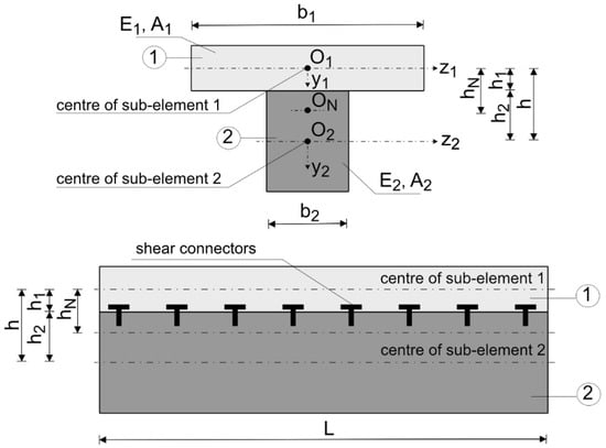
Figure 1. Geometry of the transverse section and longitudinal section of the two-layer element.

The state of the longitudinal displacements, together with the mutual displacement of the layers and the cross-sectional forces acting on the infinitesimal fragment of the beam, are shown in Figure 2a and Figure 2b, respectively.

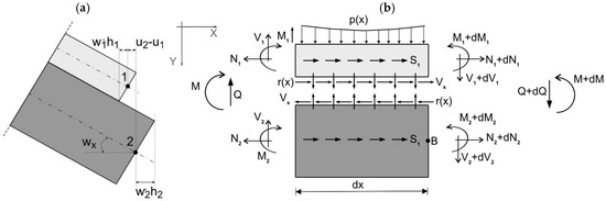
Figure 2. (a) Mutual displacements of the components of a two-layer beam. (b) Internal forces in the cross-section of a two-layer beam and at the contact zone between component layers (along section dx).

The slippage between the layers in relation to each other amounts to the following equation:

$$u_s(x)=u_2(x)-u_1(x)+h{\displaystyle \frac{dw(x)}{dx}},$$

(1)

where $h=h_1+h_2$.

The tangential forces acting on the beam in the plane of the connection (shear forces) are therefore defined by the following formula:

$$V_s\left(x\right)=k_s{u}_s\left(x\right)=k_s\left[u_2\left(x\right)-u_1\left(x\right)+h{\displaystyle \frac{dw\left(x\right)}{dx}}\right],$$

(2)

where constant k_s is the shear stiffness of the connection between both layers.

From the equilibrium equations for the selected element of a beam, the following relations are obtained.

• $\mathsf{\Sigma }X=0$

$$\begin{array}{cc}- \mathrm{for} \mathrm{the} \mathrm{upper} \mathrm{beam}& - \mathrm{for} \mathrm{the} \mathrm{lower} \mathrm{beam}\\ {\displaystyle \frac{d{N}_1\left(x\right)}{dx}}+k_s{u}_s\left(x\right)=0,& {\displaystyle \frac{d{N}_2\left(x\right)}{dx}}-k_s{u}_s\left(x\right)=0.\end{array}$$

(3)

• $\mathsf{\Sigma }Y=0$

$$\begin{array}{cc}- \mathrm{for} \mathrm{the} \mathrm{upper} \mathrm{beam}& - \mathrm{for} \mathrm{the} \mathrm{lower} \mathrm{beam}\\ {\displaystyle \frac{d{V}_1\left(x\right)}{dx}}=-p\left(x\right)+r\left(x\right),& {\displaystyle \frac{d{V}_2\left(x\right)}{dx}}=-r\left(x\right),\end{array}$$

(4)

which, when added together, becomes the following equation:

$${\displaystyle \frac{dV\left(x\right)}{dx}}=-p\left(x\right),V\left(x\right)=V_1\left(x\right)+V_2\left(x\right).$$

(5)

• $\mathsf{\Sigma }M=0$

$$\begin{array}{cc}- \mathrm{for} \mathrm{the} \mathrm{upper} \mathrm{beam}& - \mathrm{for} \mathrm{the} \mathrm{lower} \mathrm{beam}\\ V_1\left(x\right)={\displaystyle \frac{d{M}_1\left(x\right)}{dx}}+V_s\left(x\right){·h}_1,& V_2\left(x\right)={\displaystyle \frac{d{M}_2\left(x\right)}{dx}}+V_s\left(x\right){·h}_2,\end{array}$$

(6)

which, when added together, becomes the following equation:

$$V\left(x\right)={\displaystyle \frac{d{M}_B\left(x\right)}{dx}}+V_s\left(x\right)·h,M_B(x)=M_1(x)+M_2(x).$$

(7)

For the Bernoulli–Euler beam, the following constitutive relations are valid:

$$M_1\left(x\right)=-E{I}_1{\displaystyle \frac{d^2{w}_1\left(x\right)}{d{x}^2}},M_2\left(x\right)=-E{I}_2{\displaystyle \frac{d^2{w}_2\left(x\right)}{d{x}^2}},$$

(8)

and

$$N_1\left(x\right)=E{A}_1{\displaystyle \frac{d{u}_1\left(x\right)}{dx}},N_2\left(x\right)=E{A}_2{\displaystyle \frac{d{u}_2\left(x\right)}{dx}}.$$

(9)

When considering the fact that $w_1\left(x\right)=w_2\left(x\right)=w\left(x\right)$ (condition of consistency of displacements that are perpendicular to the beam’s axis), the following equation is obtained.

$$M_B\left(x\right)=M_1\left(x\right)+M_2\left(x\right)=-EI{\displaystyle \frac{d^{2}w\left(x\right)}{d{x}^2}}$$

(10)

where $EI={EI}_1+{EI}_2$.

After using dependencies (5), and Formulas (7) and (10), the following equation is obtained.

$${\displaystyle \frac{dV\left(x\right)}{dx}}={\displaystyle \frac{d^2{M}_B(x)}{d{x}^2}}+h{\displaystyle \frac{d{V}_s(x)}{dx}}=-p\left(x\right).$$

(11)

By substituting relationships (8) and (10) into equilibrium Equations (3) and (11), the following displacement equations describing the analysed model of the double-layer beam can be obtained as follows:

$$\left\{\begin{array}{c}EI{\displaystyle \frac{d^{4}w\left(x\right)}{d{x}^4}}+h{k}_s{\displaystyle \frac{d{u}_1\left(x\right)}{dx}}-h{k}_s{\displaystyle \frac{d{u}_2\left(x\right)}{dx}}-h^2{k}_s{\displaystyle \frac{d^{2}w\left(x\right)}{d{x}^2}}=p\left(x\right)\\ E{A}_1{\displaystyle \frac{d^2{u}_1\left(x\right)}{d{x}^2}}+k_s{u}_2\left(x\right)-k_s{u}_1\left(x\right)+h{k}_s{\displaystyle \frac{dw\left(x\right)}{dx}}=-s_1\\ E{A}_2{\displaystyle \frac{d^2{u}_2\left(x\right)}{d{x}^2}}-k_s{u}_2\left(x\right)+k_s{u}_1\left(x\right)-h{k}_s{\displaystyle \frac{dw\left(x\right)}{dx}}=-s_2.\end{array}\right.$$

(12)

The quantities s_1 and s_2 appearing in Equation (12) are distributed tangential loads acting in the beams’ axes (see Figure 2b).

Internal forces are defined by the following formulas (see [26]):

• The bending moment (calculated with respect to the axis z passing through point $O_N$, (see Figure 1)):

$$M\left(x\right)=M_{\mathrm{B}}\left(x\right)+M_{\mathrm{N}}\left(x\right),$$

(13)

where

$$M_B\left(x\right)=M_1\left(x\right)+M_2\left(x\right),$$

$$M_N\left(x\right)=-N_1\left(x\right)h+N\left(x\right)\left(h-h_N\right),{N\left(x\right)=N}_1\left(x\right)+N_2\left(x\right),$$

(14)

and $h_N$ determines the position of point $O_N$ in relation to the centre of the upper layer (Figure 1) at which the applied axial force generates only axial forces and does not generate bending moments in the cross-section. Distance $h_N$ is defined by the following formula:

$$h_N={\displaystyle \frac{E{A}_2}{E{A}_1+E{A}_2}}h$$

(15)

• Shear forces:

$$Q\left(x\right)=V_1\left(x\right)+V_2\left(x\right)={\displaystyle \frac{d{M}_B\left(x\right)}{dx}}+V_s\left(x\right)h=V_{\mathrm{B}}\left(x\right)+V_{\mathrm{N}}\left(x\right).$$

(16)

In the case of the action of external concentrated forces N, which are tangent to the beam’s axis and applied to the beam at point $O_N$ (see Figure 1), their distribution into the upper and lower layers is defined by the following formula:

$$N_1={\displaystyle \frac{E{A}_1}{E{A}_1+E{A}_2}}N,N_2={\displaystyle \frac{E{A}_2}{E{A}_1+E{A}_2}}N.$$

(17)

3. Solution of the Problem

The subject of the considerations in this paper are sandwich beams with static schemes that meet the following support conditions: both ends of the beam cannot move in the direction perpendicular to the beam’s axis, and at least one of the beam’s ends is supported by a pinned/roller support (in further considerations it is assumed that the beam has a roller/pinned support at its right end). This method of supporting a beam is described by the following boundary conditions:

$$w\left(0\right)=w\left(L\right)=0,{\left.{\displaystyle \frac{d^{2}w\left(x\right)}{d{x}^2}}\right|}_{x=L}=M_L,$$

(18)

Due to the assumed conditions of compatibility of displacements $w_1\left(x\right)=w_2\left(x\right)=w\left(x\right),$ conditions (18) apply to the upper and lower beams. The remaining conditions can be arbitrary, but with one proviso: a system with these conditions must be geometrically invariant. The subject of further considerations will be systems with the following static schemes (see Figure 3). However, these schemes do not contain information about the constraints that take away the possibilities of displacements of each layer in the direction tangential to the beam’s axis. In the case of the P-P scheme, in addition to conditions (18) and the following condition,

$${\left.{\displaystyle \frac{d^{2}w\left(x\right)}{d{x}^2}}\right|}_{x=0}=M_0,$$

(19)

the following additional boundary conditions are possible:

$$\begin{gathered} U_1\left(0,y_1\right)=0{\mathrm{o}\mathrm{r}\left.\partial u_1\left(x\right)/\partial x\right|}_{x=0}=0\vee N_{1,0}/{EA}_1, \\ {U}_1\left(L,y_1\right)=0{\mathrm{o}\mathrm{r}\left.\partial u_1\left(x\right)/\partial x\right|}_{x=L}=0\vee N_{1,L}/{EA}_1, \\ {U}_2\left(0,y_2\right)=0{\mathrm{o}\mathrm{r}\left.\partial u_2\left(x\right)/\partial x\right|}_{x=0}=0\vee N_{2,0}/{EA}_2, \\ {U}_2\left(L,y_2\right)=0{\mathrm{o}\mathrm{r}\left.\partial u_2\left(x\right)/\partial x\right|}_{x=L}=0\vee N_{2,L}/{EA}_2, \end{gathered}$$

(20)

where $U_i\left(x,y_i\right)=u_i\left(x,y_i\right)-{\displaystyle \frac{\partial w\left(x\right)}{\partial x}} y_{i }, -h_i\le y_i\le h_i , i=1, 2.$

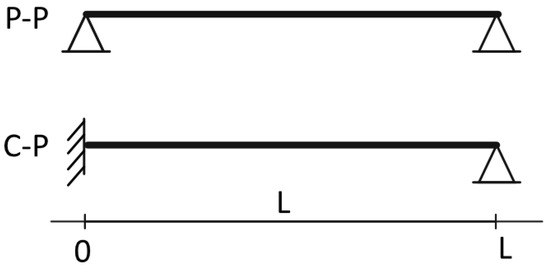
Figure 3. The analysed static diagrams.

Moments M_0 and M_L in Formulas (18) and (19) are the sums of the applied concentrated moments, and/or those that are the moment reaction to the beam’s deformation at the left and right ends of the beam, respectively. At least one of the conditions must have the form of $u_i\left(0/L\right)=0.$

In the case of the C-P scheme, in addition to conditions (18) and the following conditions,

$${\left.{\displaystyle \frac{dw\left(x\right)}{dx}}\right|}_{x=0}=0, u_1\left(0\right)=0, u_2\left(0\right)=0,$$

(21)

the following additional boundary conditions are possible:

$$\begin{array}{c}{U}_1\left(L,y_1\right)=0{\mathrm{o}\mathrm{r}\left.\partial u_1\left(x\right)/\partial x\right|}_{x=L}=0\vee N_{1,L}/{EA}_1\\ U_2\left(L,y_2\right)=0{\mathrm{o}\mathrm{r}\left.\partial u_2\left(x\right)/\partial x\right|}_{x=L}=0\vee N_{2,L}/{EA}_2\end{array}$$

(22)

The analysed problem will be solved by expanding the searched functions into Fourier series. With such defined boundary conditions (see Formula (18)), the displacement functions in the form of the following series are considered.

$$\begin{gathered} u_1\left(x\right)=\sum _{n=0}^{\mathrm{\infty }}’ u_{1n}\cos {\alpha }_{n}x, \\ {u}_2\left(x\right)=\sum _{n=0}^{\mathrm{\infty }}\begin{array}{c}’\\ \end{array}{u}_{2n}\cos {\alpha }_{n}x, \\ w\left(x\right)=\sum _{n=1}^{\mathrm{\infty }}{w}_n\sin {\alpha }_{n}x, \end{gathered}$$

(23)

where ${\alpha }_n={\displaystyle \frac{n\pi }{L}},{\displaystyle \sum _{n=0}^{\mathrm{\infty }}}\begin{array}{c}’\\ \end{array}{a}_n={\displaystyle \frac{1}{2}}{a}_0+{\displaystyle \sum _{n=1}^{\mathrm{\infty }}}{a}_n.$

After substituting the above expansions of functions $u_1, u_2,$ $\mathrm{a}\mathrm{n}\mathrm{d} w,$ and the expansions of their derivatives $u_1^{’}, u_2^{’}, u_1^{’’}, u_2^{’’}, w^{’}, w^{’’}, \mathrm{a}\mathrm{n}\mathrm{d} w^{IV}$ (see Formulas (A2)–(A6)) into the system of differential Equation (12), and by comparing the coefficients on the left and right sides of this system, an infinite system of algebraic equations is obtained as follows:

$$\left\{\begin{array}{c}EI{\alpha }_n^4{w}_n-h{k}_s{\alpha }_n{u}_{1n}+h{k}_s{\alpha }_n{u}_{2n}+h^2{k}_s{\alpha }_n^2{w}_n=p_n-EI{\displaystyle \frac{2}{L}}{\alpha }_n^3\left[{\left(-1\right)}^{n}w\left(L\right)-w\left(0\right)\right]\\ +EI{\displaystyle \frac{2}{L}}{\alpha }_n\left[{\left(-1\right)}^n{w}^{\mathrm{’}\mathrm{’}}\left(L\right)-w^{\mathrm{’}\mathrm{’}}\left(0\right)\right]+h^2{k}_s{\displaystyle \frac{2}{L}}{\alpha }_n\left[{\left(-1\right)}^{n}w\left(L\right)-w\left(0\right)\right],\\ \begin{array}{c}-E{A}_1{\alpha }_n^2{u}_{1n}+k_s{u}_{2n}-k_s{u}_{1n}+h{k}_s{\alpha }_n{w}_n=-s_{1n}-E{A}_1{\displaystyle \frac{2}{L}}\left[{\left(-1\right)}^n{u}_1^{\mathrm{’}}\left(L\right)-u_1^{\mathrm{’}}\left(0\right)\right]\\ \begin{array}{c}-h{k}_s{\displaystyle \frac{2}{L}}\left[{\left(-1\right)}^{n}w\left(L\right)-w\left(0\right)\right],\\ \begin{array}{c}-E{A}_2{\alpha }_n^2{u}_{2n}-k_s{u}_{2n}+k_s{u}_{1n}-h{k}_s{\alpha }_n{w}_n=-s_{2n}-E{A}_2{\displaystyle \frac{2}{L}}\left[{\left(-1\right)}^n{u}_2^{\mathrm{’}}\left(L\right)-u_2^{\mathrm{’}}\left(0\right)\right]\\ \begin{array}{c}+h{k}_s{\displaystyle \frac{2}{L}}\left[{\left(-1\right)}^{n}w\left(L\right)-w\left(0\right)\right];\\ \begin{array}{c}\mathrm{f}\mathrm{o}\mathrm{r}n\ge 0\end{array}.\end{array}\end{array}\end{array}\end{array}\end{array}\right.$$

(24)

Taking into account boundary conditions (18) in Equations (24), the following is obtained.

$$\left\{\begin{array}{c}\begin{array}{c}EI{\alpha }_n^4{w}_n-h{k}_s{\alpha }_n{u}_{1n}+h{k}_s{\alpha }_n{u}_{2n}+h^2{k}_s{\alpha }_n^2{w}_n=p_n-EI{\displaystyle \frac{2}{L}}{\alpha }_n{(w}^{\mathrm{’}\mathrm{’}}\left(0\right)-{\left(-1\right)}^{n}w\mathrm{’}\mathrm{’}(L)),\end{array}\\ \begin{array}{c}-E{A}_1{\alpha }_n^2{u}_{1n}+k_s{u}_{2n}-k_s{u}_{1n}+h{k}_s{\alpha }_n{w}_n=\\ \begin{array}{c}=-s_{1\mathrm{n}}+E{A}_1{\displaystyle \frac{2}{L}}\left(u_1^{\mathrm{’}}(0)-{{\left(-1\right)}^{n}u}_1^{\mathrm{’}}\left(L\right)\right),\end{array}\end{array}\\ \begin{array}{c}-E{A}_2{\alpha }_n^2{u}_{2n}-k_s{u}_{2n}+k_s{u}_{1n}-h{k}_s{\alpha }_n{w}_n=\\ =-s_{2\mathrm{n}}+E{A}_2{\displaystyle \frac{2}{L}}\left(u_2^{\mathrm{’}}(0)-{{\left(-1\right)}^{n}u}_2^{\mathrm{’}}\left(L\right)\right),\end{array}\end{array}\right.$$

(25)

when $n\ge 1$;

• $\mathrm{w}\mathrm{h}\mathrm{e}\mathrm{r}\mathrm{e}{p}_n={\displaystyle \frac{2}{L}}{\int }_0^{L}p\left(x\right)\sin {\alpha }_{n}xdx,s_{in}={\displaystyle \frac{2}{L}}{\int }_0^L{s}_1\left(x\right)\cos {\alpha }_{n}xdx,i=1, 2,$

$${ u}_{\mathrm{j}}^{\mathrm{’}}\left(0/L\right)={\left.{\displaystyle \frac{d{u}_{\mathrm{j}}\left(x\right)}{dx}}\right|}_{x=0/L}, \mathrm{w}\mathrm{’}\mathrm{’}\left(0/L\right)={\left.{\displaystyle \frac{d^2\mathrm{w}\left(x\right)}{d{x}^2}}\right|}_{x=0/L}.$$

When $n=0$, the following is obtained:

$$\left\{\begin{array}{c}{k}_s{u}_{20}-k_s{u}_{10}=-s_{10}+E{A}_1{\displaystyle \frac{2}{L}}{(u}_1^{\mathrm{’}}(0)-{{\left(-1\right)}^{n}u}_1^{\mathrm{’}}(L))\\ -k_s{u}_{20}+k_s{u}_{10}=-s_{20}+E{A}_2{\displaystyle \frac{2}{L}}\left(u_2^{\mathrm{’}}(0)-{{\left(-1\right)}^{n}u}_2^{\mathrm{’}}\left(L\right)\right) ,\end{array}\right.$$

(26)

As a result of solving the system of algebraic Equation (25), the following is obtained.

$$\begin{gathered} u_{in}=W_0^{\mathrm{”}}{u}_{in}^W-{\left(-1\right)}^n{W}_L^{\mathrm{”}}{u}_{in}^W+U_{\mathrm{1,0}}^{’}{u}_{in}^{N_1}-(-1{)}^n{U}_{1,L}^{’}{u}_{in}^{N_1}+U_{\mathrm{2,0}}^{’}{u}_{in}^{N_2}-(-1{)}^n{U}_{2,L}^{’}{u}_{in}^{N_2}+u_{in}^S , \\ i=\mathrm{1,2} \end{gathered}$$

(27)

$$w_n=W_0^{\mathrm{”}}{w}_n^W-{(-1)}^n{W}_L^{\mathrm{”}}{w}_n^W+U_{\mathrm{1,0}}^{\mathrm{’}}{w}_n^{N_1}-(-1{)}^n{U}_{1,L}^{\mathrm{’}}{w}_n^{N_1}+U_{\mathrm{2,0}}^{\mathrm{’}}{w}_n^{N_2}-(-1{)}^n{U}_{2,L}^{\mathrm{’}}{w}_n^{N_2}+w_n^S$$

where

$$\begin{array}{c}{U}_{i,0}^{\mathrm{’}}={\displaystyle \frac{2E{A}_i}{L}}{u}_i^{\mathrm{’}}\left(0\right),U_{i,L}^{’}={\displaystyle \frac{2E{A}_i}{L}}{u}_i^{\mathrm{’}}\left(L\right),i=1,W_0^{\mathrm{”}}={\displaystyle \frac{2EI}{L}}w\mathrm{”}\left(0\right),W_L^{\mathrm{”}}={\displaystyle \frac{2EI}{L}}w\mathrm{”}(L)\\ M_n=\left(\left(E{A}_1+E{A}_2\right)EI+E{A}_{1}E{A}_2{h}^2\right)k_s{L}^2{n}^2{\pi }^2+E{A}_{1}E{A}_{2}EI{n}^4{\pi }^4,\\ u_{1n}^W=-E{A}_{2}h{k}_s{L}^4/M_n,\\ u_{1n}^{N_1}=-\left(\left(EI+E{A}_2{h}^2\right)k_s{L}^4+E{A}_{2}EI{L}^2{n}^2{\pi }^2\right)/M_n.\\ u_{1n}^{N_2}=-EI{k}_s{L}^4/M_n,\\ u_{1n}^S=E{A}_{2}h{k}_s{L}^5{p}_n/\left(n\pi \cdot M_n\right)+\left(\left(EI+E{A}_2{h}^2\right)k_s{L}^4+E{A}_{2}EI{L}^2{n}^2{\pi }^2{s}_{1n}+EI{k}_s{L}^4{s}_{2n}\right)/M_n,\\ u_{2n}^W=E{A}_{1}h{k}_s{L}^4/M_n,\\ u_{2n}^{N_1}=-EI{k}_s{L}^4/M_n,\\ u_{2n}^{N_2}=-\left(\left(EI+E{A}_1{h}^2\right)k_s{L}^4+E{A}_{1}EI{L}^2{n}^2{\pi }^2\right)/M_n,\\ u_{2n}^S=-E{A}_{1}h{k}_s{L}^5{p}_n/\left(n\pi \cdot M_n\right)+\left(EI{k}_s{L}^4{s}_{1n}+\left(EI+E{A}_1{h}^2\right)k_s{L}^4+E{A}_{1}EI{L}^2{n}^2{\pi }^2{s}_{2n}\right)/M_n,\\ w_n^W=-\left(\left(E{A}_1+E{A}_2\right)k_s{L}^5+E{A}_{1}E{A}_{2}EI{L}^3{n}^2{\pi }^2\right)/\left(n\pi \cdot M_n\right),\\ w_n^{N_1}=-E{A}_{2}h{k}_s{L}^5/\left(n\pi \cdot M_n\right),\\ w_n^{N_2}=E{A}_{1}h{k}_s{L}^5/\left(n\pi \cdot M_n\right),\\ w_n^S=\left(\left(E{A}_1+E{A}_2\right)k_s{L}^6+E{A}_{1}E{A}_2{L}^4{n}^2{\pi }^2\right) p_n/\left(n^2{\pi }^2\cdot M_n\right)\\ +h{k}_s{L}^5\left(E{A}_2{s}_{1n}-E{A}_1{s}_{2n}\right)/\left(n\pi \cdot M_n\right).\end{array}$$

(28)

The formulas defining the values of concentrated moments M_0 and M_L, which were applied at the beam’s ends, require a detailed discussion (see Formulas (18) and (19)). In the case when the support system allows free displacement in the direction tangential to the beam’s axis at one of the beam’s ends, these moments are external concentrated moments applied at the beam’s ends $M_0=M_o^Z , M_L=M_L^Z$. However, when the support system prevents displacements tangential to the beam’s axis at both ends, additional moments are generated from reactions that are parallel to the beam’s axis and which occur at the supports. In the case when the direction of horizontal reactions does not coincide with the beam’s axes, these moments are defined by the following formulas:

$$\begin{gathered} M_0=M_o^Z+\left(N_1\left(0\right)-N_1\right) y_{1,0}+\left(N_2\left(0\right)-N_2\right) y_{2,0} , \\ {M}_L=M_L^Z+\left(N_1\left(L\right)-N_1\right) y_{1,L}+\left(N_2\left(L\right)-N_2\right) y_{2,L} \end{gathered}$$

(29)

In order to determine constants $u_{10},u_{20},W_0^{”}, W_L^{”},U_{i,0}^{’},U_{i,L}^{’};i=1,2$, the following system of Equations (29) resulting from the imposed boundary conditions should be solved.

$$\left[\begin{array}{ccccccc}-k_s& k_s& 0& -1& 1& 0& 0\\ k_s& -k_s& 0& 0& 0& -1& 1\\ 0& 0& S_{\partial w}^{W^{+}}& S_{\partial w}^{N_1^{+}}-{\delta ·y}_{1,0}{S}_{\partial w}^{W^{+}}& -S_{\partial w}^{N_1^{-}}+{y_{1,L}S}_{\partial w}^{W^{-}}& S_{\partial w}^{N_2^{+}}-{\delta ·y}_{2,0}{S}_{\partial w}^{W^{+}}& -S_{\partial w}^{N_2^{-}}+{y_{2,L}S}_{\partial w}^{W^{-}}\\ {\displaystyle \frac{1}{2}}& 0& S_{u_1}^{W^{+}}& S_{u_1}^{N_1^{+}}-y_{1,0}{S}_{\partial w}^{N_1^{+}}-{\delta ·y}_{1,0}{S}_{u_1}^{W^{+}}& -S_{u_1}^{N_1^{-}}+y_{1,0}{S}_{\partial w}^{N_1^{-}}+y_{1,L}{S}_{u_1}^{W^{-}}& S_{u_1}^{N_2^{+}}-y_{1,0}{S}_{\partial w}^{N_2^{+}}-{\delta ·y}_{2,0}{S}_{u_1}^{W^{+}}& -S_{u_1}^{N_2^{-}}+y_{1,0}{S}_{\partial w}^{N_2^{-}}{+y}_{2,L}{S}_{u_1}^{W^{-}}\\ {\displaystyle \frac{1}{2}}& 0& S_{u_1}^{W^{-}}& S_{u_1}^{N_1^{-}}-y_{1,L}{S}_{\partial w}^{N_1^{-}}-{\delta ·y}_{1,0}{S}_{u_1}^{W^{-}}& -S_{u_1}^{N_1^{+}}+y_{1,L}{S}_{\partial w}^{N_1^{+}}+y_{1,L}{S}_{u_1}^{W^{+}}& S_{u_1}^{N_2^{-}}-y_{1,L}{S}_{\partial w}^{N_2^{-}}-{\delta ·y}_{2,0}{S}_{u_1}^{W^{-}}& -S_{u_1}^{N_2^{+}}+y_{1,L}{S}_{\partial w}^{N_2^{+}}{+y}_{2,L}{S}_{u_1}^{W^{+}}\\ 0& {\displaystyle \frac{1}{2}}& S_{u_2}^{W^{+}}& S_{u_2}^{N_1^{+}}-y_{2,0}{S}_{\partial w}^{N_1^{+}}-{\delta ·y}_{1,0}{S}_{u_2}^{W^{+}}& -S_{u_2}^{N_1^{-}}+y_{2,0}{S}_{\partial w}^{N_1^{-}}+y_{1,L}{S}_{u_2}^{W^{-}}& S_{u_2}^{N_2^{+}}-y_{2,0}{S}_{\partial w}^{N_2^{+}}-{\delta ·y}_{2,0}{S}_{u_2}^{W^{+}}& -S_{u_2}^{N_2^{-}}+y_{2,0}{S}_{\partial w}^{N_2^{-}}{+y}_{2,L}{S}_{u_2}^{W^{-}}\\ 0& {\displaystyle \frac{1}{2}}& S_{u_2}^{W^{-}}& S_{u_2}^{N_1^{-}}-y_{2,L}{S}_{\partial w}^{N_1^{-}}-{\delta ·y}_{1,0}{S}_{u_2}^{W^{-}}& -S_{u_2}^{N_1^{+}}+y_{2,L}{S}_{\partial w}^{N_1^{+}}+y_{1,L}{S}_{u_2}^{W^{+}}& S_{u_2}^{N_2^{-}}-y_{2,L}{S}_{\partial w}^{N_2^{-}}-{\delta ·y}_{2,0}{S}_{u_2}^{W^{-}}& -S_{u_2}^{N_2^{+}}+y_{2,L}{S}_{\partial w}^{N_2^{+}}{+y}_{2,L}{S}_{u_2}^{W^{+}}\end{array}\right] \left[\begin{array}{c}{u}_{10}\\ u_{20}\\ W_0^{”}\\ U_{1,0}^{’}\\ U_{1,L}^{’}\\ U_{2,0}^{’}\\ U_{2,L}^{’}\end{array}\right]=$$

$$-\left[\begin{array}{c}{s}_{10}\\ s_{20}\\ S_{\partial w}^{S^{+}}-\delta ·S_{\partial w}^{W^{+}}{\displaystyle \frac{2}{L}}\left(M_0^F-N_{1 }{y}_{1,0}-N_{2 }{y}_{2,0}\right)+S_{\partial w}^{W^{-}}{\displaystyle \frac{2}{L}}(M_L^F-N_{1 }{y}_{1,L}-N_{2 }{y}_{2,L})\\ S_{u_1}^{S^{+}}-y_{1,0}{S}_{\partial w}^{S^{+}}-{\delta ·S}_{u_1}^{W^{+}}{\displaystyle \frac{2}{L}}\left(M_0^F-N_{1 }{y}_{1,0}-N_{2 }{y}_{2,0}\right)+S_{u_1}^{W^{-}}{\displaystyle \frac{2}{L}}(M_L^F-N_{1 }{y}_{1,L}-N_{2 }{y}_{2,L})\\ S_{u_1}^{S^{-}}-y_{1,L}{S}_{\partial w}^{S^{-}}-{\delta ·S}_{u_1}^{W^{-}}{\displaystyle \frac{2}{L}}\left(M_0^F-N_{1 }{y}_{1,0}-N_{2 }{y}_{2,0}\right)+S_{u_1}^{W^{+}}{\displaystyle \frac{2}{L}}(M_L^F-N_{1 }{y}_{1,L}-N_{2 }{y}_{2,L})\\ S_{u_2}^{S^{+}}-y_{2,0}{S}_{\partial w}^{S^{+}}-{\delta ·S}_{u_2}^{W^{+}}{\displaystyle \frac{2}{L}}\left(M_0^F-N_{1 }{y}_{1,0}-N_{2 }{y}_{2,0}\right)+S_{u_2}^{W^{-}}{\displaystyle \frac{2}{L}}(M_L^F-N_{1 }{y}_{1,L}-N_{2 }{y}_{2,L})\\ S_{u_2}^{S^{-}}-y_{2,L}{S}_{\partial w}^{S^{-}}-{\delta ·S}_{u_2}^{W^{-}}{\displaystyle \frac{2}{L}}\left(M_0^F-N_{1 }{y}_{1,0}-N_{2 }{y}_{2,0}\right)+S_{u_2}^{W^{+}}{\displaystyle \frac{2}{L}}(M_L^F-N_{1 }{y}_{1,L}-N_{2 }{y}_{2,L})\end{array}\right]\begin{array}{c} \left(\mathrm{E}\mathrm{q}\mathrm{u}\mathrm{a}\mathrm{t}\mathrm{i}\mathrm{o}\mathrm{n}\right(26\left)\right)\\ \left(\mathrm{E}\mathrm{q}\mathrm{u}\mathrm{a}\mathrm{t}\mathrm{i}\mathrm{o}\mathrm{n}\right(26\left)\right)\\ (w’(0)=0)\\ \left(u_1\right(0)=0)\\ \left(u_1\right(L)=0)\\ \left(u_2\right(0)=0)\\ \left(u_2\right(L)=0)\end{array}; \delta =\left\{\begin{array}{c}1 \mathrm{f}\mathrm{o}\mathrm{r}\mathrm{P}-\mathrm{P}\mathrm{b}\mathrm{e}\mathrm{a}\mathrm{m}\\ 0 \mathrm{f}\mathrm{o}\mathrm{r}\mathrm{C}-\mathrm{P}\mathrm{b}\mathrm{e}\mathrm{a}\mathrm{m}\end{array}\right.$$

(30)

where

$$\begin{array}{c}{S_{u_1}^{W^{+}}={\displaystyle \sum _{n=1}}{u}_{1n}^W,S}_{u_1}^{W^{-}}={\displaystyle \sum _{n=1}}(-1{)}^n{u}_{1n}^W,S_{u_1}^{N_1^{+}}={\displaystyle \sum _{n=1}}{u}_{1n}^W,S_{u_1}^{N_1^{-}}={\displaystyle \sum _{n=1}}(-1{)}^n{u}_{1n}^{N_1},\\ S_{u_1}^{N_2^{+}}={\displaystyle \sum _{n=1}}{u}_{1n }^{N_2},S_{u_1}^{N_2^{-}}={\displaystyle \sum _{n=1}}(-1{)}^n{u}_{1n}^{N_2},{S_{u_1}^{S^{+}}={\displaystyle \sum _{n=1}}{u}_{1n}^S, S}_{u_1}^{S^{-}}={\displaystyle \sum _{n=1}}(-1{)}^n{u}_{1n}^S, \\ {S_{u_2}^{W^{+}}={\displaystyle \sum _{n=1}}{u}_{2n}^W,S}_{u_2}^{W^{-}}={\displaystyle \sum _{n=1}}(-1{)}^n{u}_{2n}^W,{S_{u_2}^{N_1^{+}}={\displaystyle \sum _{n=1}}{u}_{2n}^{N_1},S}_{u_2}^{N_1^{-}}={\displaystyle \sum _{n=1}}(-1{)}^n{u}_{2n}^{N_1}, \\ S_{u_2}^{N_2^{+}}={\displaystyle \sum _{n=1}}{u}_{2n}^{N_2},S_{u_2}^{N_2^{-}}={\displaystyle \sum _{n=1}}(-1{)}^n{u}_{2n}^{N_2},{S_{u_2}^{S^{+}}={\displaystyle \sum _{n=1}}{u}_{2n}^S,S}_{u_2}^{S^{-}}={\displaystyle \sum _{n=1}}(-1{)}^n{u}_{2n}^S, \\ S_{\partial w}^{W^{+}}={\displaystyle \sum _{n=1}}{\alpha }_n{w}_n^W,S_{\partial w}^{W^{-}}={\displaystyle \sum _{n=1}}{(-1{)}^n\alpha }_n{w}_n^W, \\ S_{\partial w}^{N_1^{+}}={\displaystyle \sum _{n=1}}{\alpha }_n{w}_n^{N_1},S_{\partial w}^{N_1^{-}}={\displaystyle \sum _{n=1}}(-1{)}^n{\alpha }_n{w}_n^{N_1},\\ {S_{\partial w}^{N_2^{+}}={\displaystyle \sum _{n=1}}{\alpha }_n{w}_n^{N_2}, S}_{\partial w}^{N_2^{-}}={\displaystyle \sum _{n=1}}(-1{)}^n{\alpha }_n{w}_n^{N_2},\\ S_{\partial w}^{S^{+}}={\displaystyle \sum _{n=1}}{\alpha }_n{w}_n^S, S_{\partial w}^{S^{-}}={\displaystyle \sum _{n=1}}(-1{)}^n{\alpha }_n{w}_n^S,{ \alpha }_n={\displaystyle \frac{n\pi }{L}}.\end{array}$$

The first two equations of this system result directly from Equations (26). The third equation is the condition assumed for the C-P beam ${\left.dw\left(x\right)/dx\right|}_{x=0}=0$ (in the case of the P-P beam, this equation should be omitted, because then the unknown of this system $W_0^{”}$ is known and is equal to $W_0^{”}=-U_{\mathrm{1,0}}^{’} y_{\mathrm{1,0}}-U_{\mathrm{2,0}}^{’} y_{\mathrm{2,0}}+{\displaystyle \frac{2}{L}}(M_0^F-N_{1 }{y}_{\mathrm{1,0}}-N_{2 }{y}_{\mathrm{2,0}})$). The omitting of the third equation in the P-P case numerically comes down to deleting the third row and the third column in the main matrix of the system of equations (30), and the third coordinate in the vector of unknowns and the vector of free terms. The remaining four equations result from the assumption that the upper and lower beams are deprived of the possibility of displacement in the direction tangential to the beam’s axis at its left and right ends. If the beam/beams has/have the possibility of displacement at their ends in this direction, then the appropriate equation should be omitted in system (29). In such a case, some of the parameters are known and are proportional to the axial forces at the beam’s ends.

The calculation of coefficients $w_n$, $u_{1n}$ and $u_{2n}$ allows the sought displacement functions to be determined, as well as—after using the relationships that define the coefficients of derivatives of these functions—the internal forces. Normal stresses ${\sigma }_x$ are determined using the following known formula:

$${\sigma }_x^i\left(y_i\right)={\displaystyle \frac{N_i}{{EA}_i}}+{\displaystyle \frac{M_i}{{EI}_i}}{y}_i$$

(31)

4. Analysis of the Influence of the Position of Support Points: Numerical Examples

The solution presented in point 3 was used to analyse the influence of the location of the beam’s support points (with a certain cross-section) on the beam’s static response. These analyses were performed while assuming different values of the stiffness (shear) of the connection between the layers. The conducted research involved two-layered wooden beams with the P-P and C-P static scheme (see Figure 3), and the cross-section that is shown in Figure 1. The dimensions of these beams were as follows: $L=2.0 \mathrm{m},b_1=0.3 \mathrm{m}, b_2=0.05 \mathrm{m}, {H_1=2h}_1=0.05 \mathrm{m},{ H_2=2h}_2=0.15 \mathrm{m}.$

The material parameters were as follows: for the P-P beams—$E_1={12\times 10^9 \mathrm{Pa}, E}_2=8\times 10^9 \mathrm{Pa}$, and for the C-P beams $E_1=E_2=10\times 10^9 \mathrm{Pa}$. The load acting on the beams was as follows:

-

In the case of the P-P beams, the load was evenly distributed over the entire length of the beam with the intensity of $q=1\mathrm{kN}/\mathrm{m}$. The coefficients of this load were developed into a sinusoidal Fourier series defined by the following formula:

$$p_n={\displaystyle \frac{2}{L}}{\int }_0^{L}q\sin {\alpha }_{n}xdx=2q{\displaystyle \frac{1-\cos n\pi }{n\pi }},n=\mathrm{1,2},3,\dots$$

(32)

-

In the case of the C-P beams, it was the concentrated force $P=1\mathrm{kN}$ applied in the middle of the span ($x=L/2)$. The expansion coefficients of this load were developed into a sinusoidal Fourier series defined by the following formula:

$$p_n={\displaystyle \frac{2}{L}}{\int }_0^{L}P\delta \left(x-{\displaystyle \frac{L}{2}}\right)\sin {\alpha }_{n}xdx={\displaystyle \frac{2P}{L}}\sin {\displaystyle \frac{n\pi }{2}},n=\mathrm{1,2},3,...$$

(33)

In the analysed examples, it was assumed that $s_1=s_2=0, N_1=N_2=0, M_0^F=M_L^F=0.$

Calculations were performed for different values of the stiffness of the connection between layers ($k_s)$ by assuming $k_s=0, { 10}^6, 5\times {10}^7, {10}^9\mathrm{P}\mathrm{a}$.

Various support variants were analysed. In order to shorten their description, the following three-letter convention was introduced in order to define the method of supporting the P-P beam:

Stj, where

S determines the position of the support and takes the values L—the support of the left beam’s end and R—the support of the right beam’s end;

t defines the type of the support and takes the values n—the support that prevents the beam from moving in the direction tangential to the beam’s axis and p—the support does not block this movement; and

j is a support point, j = 1, 2, 3, 4, 5, 6 (see Figure 4). The coordinates of each support point j = 1–6 are specified along the y-axis.

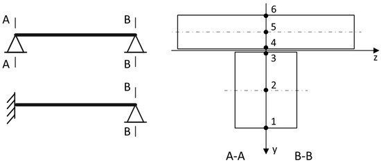
Figure 4. The analysed support points. The coordinates of support points $z_j$ = 0, j = 1, …,6.

For example: ((Ln2, Ln5), Rp1) means that the beam is supported on its left end by two pinned supports at points 2 and 5, and the right end is supported at point 1 by a roller support.

In the case of the C-P beams, the abbreviated notation convention is (C, tj), which means that at the left end, where the beam is fixed, both layers are not allowed to move tangentially to the axis of the layers, and at the right end, the beam is supported at point j by a type t support (t = p—roller support, t = n—pinned support). When it is clear from the context with which supports we are dealing with, their designations are limited to giving only the numbers of the support points, e.g., ((2, 5), 1) or (C, 1).

$$(y_1={2h}_2, y_2=h_2, y_3=0_{+}, y_4=0_{-}, y_5={-h}_1, y_6={-2h}_1).$$

In the case of the P-P beams with the possibility of free displacement in the direction tangential to the beam’s axis at its right end, the following support variants were tested.

• ((Ln2, Ln5), Rp2); ((Ln3, Ln4), R2); ((Ln1, Ln6), Rp2); (Ln2, Rp2).

In the case of the P-P beams with the possibility of free displacement in the tangential direction at both ends of the beam, the following support variants were analysed.

• (Ln j, Rn k), j = 1, …, 6; k = j, …, 6.

When analysing C-P beams with the possibility of free displacement in the direction tangential to the beam’s axis at its right end, the following support variant was tested.

• (C, p2);

When analysing the C-P beams with the possibility of free displacement in the tangential direction at the right end of the beam, the following support variants were analysed.

• (C, n j), j = 1, …, 6;

Due to the Gibbs effect, which occurs in the vicinity of the points of the discontinuity function (of the “jump” type), the exact values of the axial forces and bending moments at the beams’ ends were determined using relationships (8)–(10), (13), and (14), as well as the calculated exact values of the functions ${ { u}_1^{’}\left(0\right), u}_1^{’}\left(L\right), { { u}_2^{’}\left(0\right), u}_2^{’}\left(L\right), \mathrm{a}\mathrm{n}\mathrm{d} w^{’’}\left(0\right)$ that occur in these relationships.

The dependence between displacement $w\left(L/2\right)$ and the value of parameter $k_s\in ⟨0, 10^9⟩ \mathrm{Pa}$ for the P-P and C-P beams is shown in Figure 5. The graphs for the P-P beams show this dependence for beams with supports (Ln2, Rp2), (Ln1, Rn1), (Ln3, Rn3). In the case of the C-P beams, these graphs refer to the beams with supports (C, p2), (C, n1), (C, n3). The supports at points (1, 1) (respectively, (C, 1)) were the supports (from those analysed) for which displacements w(L⁄2) were the smallest. The supports at points (3, 3) respectively, (C, 3) were the supports for which displacements w(L⁄2) were the largest.

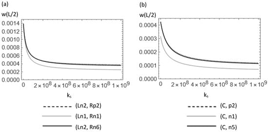
Figure 5. The dependence between displacement values $w\left(L/2\right)$ [m] and the stiffness of the layer connection $k_s$ in the case of different support methods for (a) the P-P beam and (b) the C-P beam.

The graphs of displacements w(x); the function describing the mutual slippage of layers in relation to each other $u_s\left(x\right)$; axial forces $N_1\left(x\right), { N}_2\left(x\right)$; bending moments M(x) with their components $M_B\left(x\right), { M}_N\left(x\right)$; and shear forces V(x) with their components $V_{\mathrm{B}}\left(x\right),V_{\mathrm{N}}\left(x\right)$ for $k_s=0; 10^6; 5\times 10^7 \mathrm{i} 10^{9 }\mathrm{Pa}$ and for the selected support methods are presented in Figure 6, Figure 7, Figure 8, Figure 9 and Figure 10.

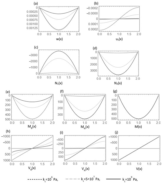
Figure 6. Graphs of (a) displacements $w\left(x\right)$ [m], (b) the mutual function of “slippage” between layers $u_s\left(x\right)$ [m], and (c,d) axial forces $N_1\left(x\right), { N}_2\left(x\right)$ [N], (e) the component of bending moments $M_B\left(x\right)$, (f) the component of bending moments $M_N\left(x\right)$, (g) bending moments $M\left(x\right)$ [Nm], (h) the component of shear forces $V_{\mathrm{N}}\left(x\right),$ (i) the component of shear forces $V_{\mathrm{N}}\left(x\right)$, and (j) shear forces $\mathrm{V}\left(x\right)$ [N] for different values of the $k_s$ parameter in the case of the P-P beams with support (Ln2, Rp2).

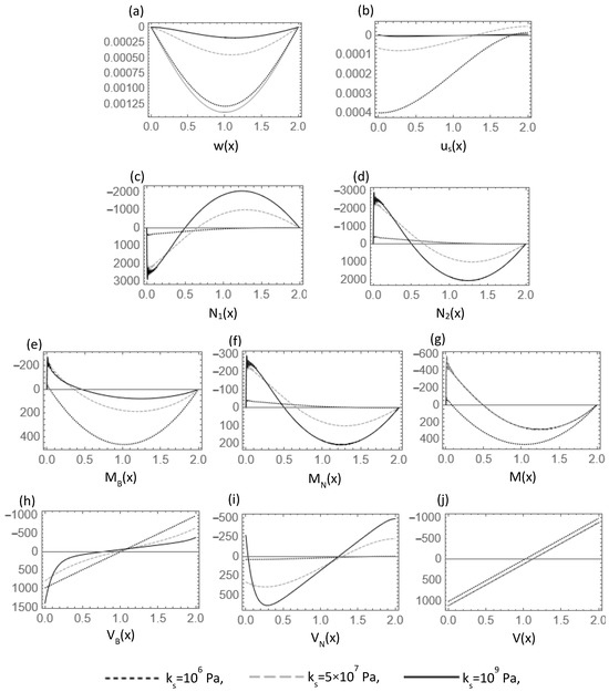
Figure 7. Graphs of (a) displacements $w\left(x\right)$ [m], (b) the mutual function of “slippage” between layers $u_s\left(x\right)$ [m], and (c,d) axial forces $N_1\left(x\right), { N}_2\left(x\right)$ [N], (e) the component of bending moments $M_B\left(x\right)$, (f) the component of bending moments $M_N\left(x\right)$, (g) bending moments $M\left(x\right)$ [Nm], (h) the component of shear forces $V_{\mathrm{N}}\left(x\right),$ (i) the component of shear forces $V_{\mathrm{N}}\left(x\right)$, and (j) shear forces $\mathrm{V}\left(x\right)$ [N] for different values of the $k_s$ parameter in the case of the P-P beams with support (Ln1,Ln6), Rp2).

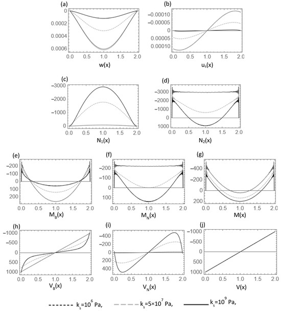
Figure 8. Graphs of (a) displacements $w\left(x\right)$ [m], (b) the mutual function of “slippage” between layers $u_s\left(x\right)$ [m], and (c,d) axial forces $N_1\left(x\right), { N}_2\left(x\right)$ [N], (e) the component of bending moments $M_B\left(x\right)$, (f) the component of bending moments $M_N\left(x\right)$, (g) bending moments $M\left(x\right)$ [Nm], (h) the component of shear forces $V_{\mathrm{N}}\left(x\right),$ (i) the component of shear forces $V_{\mathrm{N}}\left(x\right)$, and (j) shear forces $\mathrm{V}\left(x\right)$ [N] for different values of the $k_s$ parameter in the case of the P-P beams with support (Ln1, Rn1).

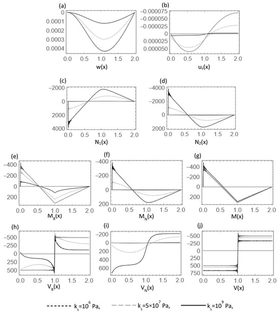
Figure 9. Graphs of (a) displacements $w\left(x\right)$ [m], (b) the mutual function of “slippage” between layers $u_s\left(x\right)$ [m], and (c,d) axial forces $N_1\left(x\right), { N}_2\left(x\right)$ [N], (e) the component of bending moments $M_B\left(x\right)$, (f) the component of bending moments $M_N\left(x\right)$, (g) bending moments $M\left(x\right)$ [Nm], (h) the component of shear forces $V_{\mathrm{N}}\left(x\right),$ (i) the component of shear forces $V_{\mathrm{N}}\left(x\right)$, and (j) shear forces $\mathrm{V}\left(x\right)$ [N] for different values of the $k_s$ parameter in the case of the C-P beams with support (C, p2).

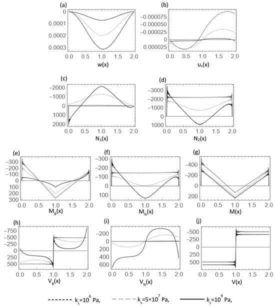
Figure 10. Graphs of (a) displacements $w\left(x\right)$ [m], (b) the mutual function of “slippage” between layers $u_s\left(x\right)$ [m], and (c,d) axial forces $N_1\left(x\right), { N}_2\left(x\right)$ [N], (e) the component of bending moments $M_B\left(x\right)$, (f) the component of bending moments $M_N\left(x\right)$, (g) bending moments $M\left(x\right)$ [Nm], (h) the component of shear forces $V_{\mathrm{N}}\left(x\right),$ (i) the component of shear forces $V_{\mathrm{N}}\left(x\right)$, and (j) shear forces $\mathrm{V}\left(x\right)$ [N] for different values of the $k_s$ parameter in the case of the C-P beams with support (C, n1).

The values of displacements w(L⁄2), bending moments $M\left(0\right),M(L⁄2),M\left(L\right)$ for $k_s=5\times {10}^7 \mathrm{P}\mathrm{a},$ and for all the analysed support methods are presented in Table 1, Table 2, Table 3, Table 4 and Table 5. Table 1 contains the results for the P-P beam with a right roller support and two pinned supports on the left side. For comparison, Table 2 presents the results for the beam that is, on the left side, supported by one pinned support and on the right end by a roller support (support (Ln2, Rp2)). Table 3 presents the results for the P-P beams with pinned supports on both ends of a beam. Table 5 shows the results for the C-P beam with the right pinned support, whereas Table 4 shows the results for the C-P beam with the right roller support.

Table 1. The P-P beam with a pinned support at the left end (two pinned supports) and a roller support at the right end.

Support	w(L/2) [m]	M(0) [Nm]	M(L/2) [Nm]	M(L) [Nm]
((3, 4), 2)	2.429 × 10−3	0	500	0
((2, 5), 2)	2.701 × 10−3	−153.08	423.71	0
((1, 6), 2)	1.780 × 10−3	−486.50	257.52	0

Table 2. The P-P beam with a pinned support at the left end (one pinned support) and a roller support at the right end.

Support	w(L/2)	M(0)	M(L/2)	M(L)
(2, 2)	2.869 × 10−3	0	500	0

Table 3. The P-P beam with a pinned support at both ends.

Support	w(L/2)	M(0)	M(L/2)	M(L)
(1, 1)	1.256 × 10−3	−360.39	140.75	−360.39
(1, 2)	1.830 × 10−3	−373.02	221.12	−186.51
(1, 3)	2.697 × 10−3	−156.41	422.04	0
(1, 4)	1.846 × 10−3	−390.91	305.17	0
(1, 5)	2.148 × 10−3	−351.03	354.2	58.505
(1, 6)	2.464 × 10−3	−271.59	409.76	90.53
(2, 2)	2.577 × 10−3	−132.94	367.48	−132.94
(2, 3)	2.785 × 10−3	70.968	535.37	0
(2, 4)	2.626 × 10−3	−130.5	434.96	0
(2, 5)	2.829 × 10−3	−54.38	481.81	18.246
(2, 6)	2.855 × 10−3	33.941	505.64	−22.628
(3, 3)	2.102 × 10−3	0	500.00	0
(3, 4)	2.737 × 10−3	0	500.00	0
(3, 5)	2.489 × 10−3	0	476.15	−47.86
(3, 6)	2.192 × 10−3	0	440.41	−119.55
(4, 4)	2.525 × 10−3	0	500	0
(4, 5)	2.839 × 10−3	0	512.45	24.979
(4, 6)	2.795 × 10−3	0	466.24	−67.733
(5, 5)	2.778 × 10−3	−41.215	458.92	−41.215
(5, 6)	2.392 × 10−3	−85.542	372.1	−171.08
(6, 6)	1.922 × 10−3	−211.61	289.06	−211.61

Table 4. The C-P beam with a roller support at the right end.

Support	w(L/2)	M(0)	M(L/2)	M(L)
(C, 2)	2.913 × 10−4	−385,23	306.79	0

Table 5. The C-P beam with a pinned support the right end.

Support	w(L/2)	M(0)	M(L/2)	M(L)
(C, 1)	2.006 × 10−4	−317.76	201.13	−279.86
(C, 2)	2.805 × 10−4	−388.65	270.95	−68,883
(C, 3)	2.580 × 10−4	−332.16	327.91	−11.077
(C, 4)	2.862 × 10−4	−375.04	315.22	6.3437
(C, 5)	2.869 × 10−4	−386.85	292.25	−27.937
(C, 6)	2.564 × 10−4	−363.20	258.50	−119.31

Since spectacular qualitative differences for the analysed beams’ support methods are visible in the bending moment diagrams M(x), their diagrams for all the support methods analysed in the paper are presented in Figure 11, Figure 12, Figure 13 and Figure 14.

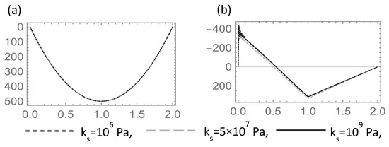
Figure 11. Bending moment diagrams $M\left(x\right)$ [Nm] for different values of the $k_s$ parameter in the case of the beam: (a) P-P z with support (Ln2, Rp2) and (b) C-P with support (C, p2).

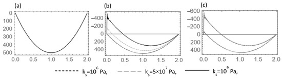
Figure 12. Bending moment diagrams $M\left(x\right)$ [Nm] for different values of the $k_s$ parameter in the case of the P-P beam: (a) with support ((Ln3, Ln4), Rp2), (b) with support ((Ln2, Ln5), Rp2), and (c) with support ((Ln1, Ln6), Rp2).

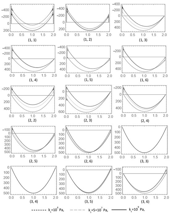
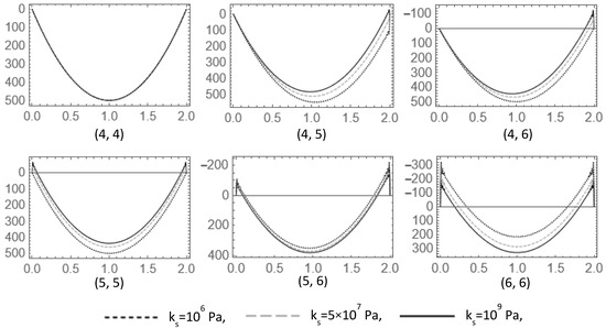
Figure 13. Bending moment diagrams $M\left(x\right)$ [Nm] for different values of the $k_s$ parameter in the case of the P-P beams with support (Ln j, Rn k), j = 1, …, 6; k = j, …, 6.

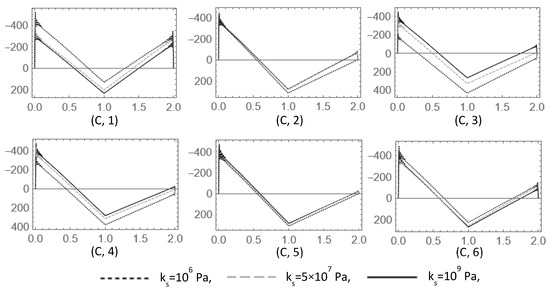
Figure 14. Bending moment diagrams $M\left(x\right)$ [Nm] for different values of the $k_s$ parameter in the case of the C-P beams with support (C, nj), j = 1, …, 6.

In order to demonstrate the significant influence of the stiffness of the connection between layers $k_s$ on the response of the system, Table 6, Table 7, Table 8, Table 9 and Table 10 compare the values of displacements w(L⁄2) and bending moments M(0), M(L⁄2), M(L), which were determined for different values of the stiffness of this connection. Calculations were performed for $k_s=0;10^6;5\times 10^7\mathrm{a}\mathrm{n}\mathrm{d}10^{9 }\mathrm{Pa}$. Table 6, Table 7, Table 8, Table 9 and Table 10 present the results for the P-P and C-P beams with the selected support methods.

Table 6. The P-P beam with a pinned support at the left end (one pinned support) and a roller support at the right end.

ks	w(L/2)	M(0)	M(L/2)	M(L)
Support (2, 2)
0	1.389 × 10−3	0	500	0
106	1.353 × 10−3	0	500	0
5 × 107	2.869 × 10−3	0	500	0
109	3.747 × 10−4	0	500	0

Table 7. The P-P beam with a pinned support at the left end (two pinned supports) and a roller support at the right end.

ks	w(L/2)	M(0)	M(L/2)	M(L)
Support ((3, 4), 2)
0	1.389 × 10−3	0	500	0
106	1.291 × 10−3	0	500	0
5 × 107	2.429 × 10−3	0	500	0
109	3.710 × 10−4	0	500	0
Support ((2, 5), 2)
0	1.389 × 10−3	0	500	0
106	1.353 × 10−3	−0.3705	499.82	0
5 × 107	2.701 × 10−3	−153.08	423.71	0
109	1.937 × 10−4	−444.4	278.51	0
Support ((1, 6), 2)
0	1.389 × 10−3	0	500	0
106	1.289 × 10−3	−78.179	461.03	0
5 × 107	1.780 × 10−3	−486.5	257.52	0
109	1.672 × 10−4	−487.11	257.22	0

Table 8. The P-P beam with a pinned support at both ends.

ks	w(L/2)	M(0)	M(L/2)	M(L)
Support (2, 2)
0	1.389 × 10−3	0	500	0
106	1.352 × 10−3	−6.483	493.54	−6.483
5 × 107	2.577 × 10−3	−132.94	367.48	−132.94
109	1.963 × 10−4	−218.99	281.7	−218.99
Support (2, 5)
0	1.389 × 10−3	0	500	0
106	1.353 × 10−3	−0.139	499.95	0.046
5 × 107	2.829 × 10−3	−54.738	481.81	18.246
109	3.355 × 10−4	−144.46	452.00	48.153
Support (5, 5)
0	1.389 × 10−3	0	500	0
106	1.352 × 10−3	−2.153	497.85	−2.153
5 × 107	2.778 × 10−3	−41.215	458.92	−41.215
109	3.223 × 10−4	−64.339	435.87	−64.339

Table 9. The C-P beam with a roller support at the right end.

ks	w(L/2)	M(0)	M(L/2)	M(L)
Support (C, 2)
0	4.226 × 10−4	−376.14	311.52	0
106	4.181 × 10−4	−373.17	313.00	0
5 × 107	2.913 × 10−4	−385.62	306.79	0
109	1.182 × 10−4	−417.23	291.03	0

Table 10. The C-P beam with a pinned support at the right end.

ks	w(L/2)	M(0)	M(L/2)	M(L)
Support (C, 2)
0	3.152 × 10−4	−452.21	124.81	−319.54
106	3.106 × 10−4	−442.63	129.65	−319.27
5 × 107	2.006 × 10−4	−317.76	201.13	−279.86
109	7.162 × 10−5	−304.26	231.68	−174.03
Support (C, 5)
0	4.226 × 10−4	−376.14	311.52	0
106	4.181 × 10−4	−375.01	311.11	−1.9406
5 × 107	2.869 × 10−4	−386.85	292.25	−27.937
109	1.140 × 10−4	−404.96	285.18	−24.008

The subject of the analyses was also the stress state of the structure. Due to the limited volume of this paper, the normal stress distribution graphs (see Formula (30)) are presented for the selected beams’ support methods (the same for which the graphs are presented in Figure 6, Figure 7, Figure 8, Figure 9 and Figure 10) and three values of parameter $k_s=0; 5\times 10^7;10^{14 }\mathrm{Pa}$. These stresses were determined at points $x=L/4$ and $x=L/2$, and in the case of C-P beams, also at the point $x=0$. The obtained results are presented in Figure 15, Figure 16, Figure 17, Figure 18 and Figure 19. In these graphs, the “0” ordinate of the vertical reference axis was assumed at the point located at the contact point between both layers.

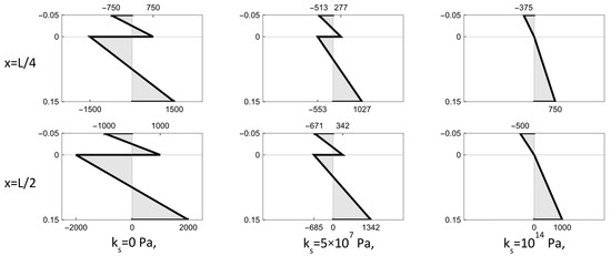
Figure 15. Normal stresses ${\sigma }_x$ [kPa] in cross-sections $x=L/4 \mathrm{a}\mathrm{n}\mathrm{d} L/2$ for different values of the $k_s$ parameter in the case of the P-P beam with support (Ln2, Rp2).

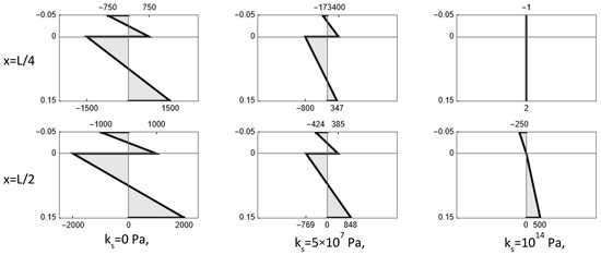
Figure 16. Normal stresses ${\sigma }_x$ [kPa] in cross-sections $x=L/4 \mathrm{a}\mathrm{n}\mathrm{d} L/2$ for different values of the $k_s$ parameter in the case of the P-P beam with support ((Ln1, Ln6), Rp2).

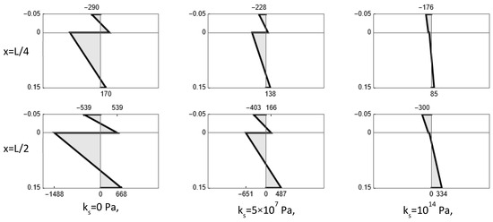
Figure 17. Normal stresses ${\sigma }_x$ [kPa] in cross-sections $x=L/4 \mathrm{a}\mathrm{n}\mathrm{d} L/2$ for different values of the $k_s$ parameter in the case of the P-P beam with support (Ln1, Rn1).

Figure 18. Normal stresses ${\sigma }_x$ kPa] in cross-sections $x=L/4 \mathrm{a}\mathrm{n}\mathrm{d} L/2$ for different values of the $k_s$ parameter in the case of the C-P beam with support (C, p2).

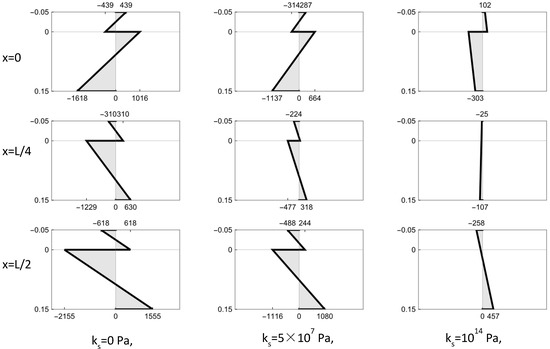
Figure 19. Normal stresses ${\sigma }_x$ [kPa] in cross-sections $x=L/4 \mathrm{a}\mathrm{n}\mathrm{d} L/2$ for different values of the $k_s$ parameter in the case of the C-P beam with support (C, n1).

For the value of $k_s=10^{14} \mathrm{Pa}$ there is practically no slippage between the layers in the beam, and the beam behaves like a monolithic beam. For the C-P beams, for which the same moduli of elasticity of layers $E_1=E_2$ were assumed, in the case of a lack of slippage (for the value of $k_s=10^{14} \mathrm{Pa}$), the normal stress graphs should have a linear course. Such a course can be seen in the presented graphs (see Figure 18 and Figure 19).

All the calculations, as well as the graphs of the functions, were performed using the Mathematica 14 programme [29].

5. Analysis of the Results

The obtained results show that the change in stiffness in the range of $⟨0, 3\times 10^8⟩ \mathrm{Pa}$ has a significant influence on the displacements w(L/2) of the two-layer system. If the difference in the displacements calculated for $k_s=0 \mathrm{Pa}$ and $k_s=10^{14 }\mathrm{Pa}$ is taken as the comparative value, then the changes in this displacement when $k_s\in ⟨0, 3\times 10^8⟩ \mathrm{Pa}$ are in the following ranges:

-

In the case of the P-P beams with the following supports:

(Ln2, Rp2)—91.67%,

(Ln1, Rn1)—88.53%,

(Ln2, Rn6)—91.01%.

-

In the case of the C-P beams with the following supports:

(C, Rp2)—83.92%,

(C, Rn1)—85.87%,

(C, Rn5)—84.34%.

In order to illustrate the influence of the beam’s supports on its static response, the ratios of the displacement function values in the middle of the beam’s span $w(L/2)$ (determined for different methods of supporting P-P beams) to the value of this function determined for the P-P beam with support (Ln2,Rp2) were calculated. Similarly, in the case of the C-P beams, the ratios of the function values $w(L/2)$, calculated for different methods of support, to the value of this function for the beam with support (C, p2) were determined. The following results were obtained.

-

In the case of the P-P beams with pinned supports at the left end (two supports) and roller supports at the right end,

((3, 4), 2)—0.85,

((2, 5), 2)—0.94,

((1, 6), 2)—0.62.

-

In the case of the P-P beams with pinned supports at both ends,

the highest value (max) was obtained for support (2, 6)—1.00,

the lowest value (min) was obtained for support (1, 1)—0.44.

-

In the case of the C-P beams with a non-sliding support at the right end,

the highest value (max) was obtained for support (C, 3)—0.98,

the lowest value (min) was obtained for support (C, 1)—0.69.

A similar comparison was made for the values of bending moments at the ends and in the middle of the beam’s span. However, the moment ratios were calculated in relation to the value of the bending moment in the middle of the beam’s P-P span with support (Ln2, Rp2), or in the middle of the beam’s C-P span with support (C, p2). The following results were obtained.

-

In the case of the P-P beams with pinned supports at the left end (two supports) and roller supports at the right end (see Table 11):

Table 11. The P-P beam with a pinned support at the left end (two pinned supports) and a roller support at the right end.

Support	M(0)	M(L/2)	M(L)
((3, 4), 2)	0.00	1.00	0.00
((2, 5), 2)	−0.31	0.85	0.00
((1, 6), 2)	−0.97	0.52	0.00

-

In the case of the P-P beams with pinned supports at both ends (see Table 12):

Table 12. The P-P beam with a pinned support at both ends.

	Support	M(0)	M(L/2)	M(L)
Max	(2, 6)	0.07	1.01	−0.05
Min	(1, 1)	−0.72	0.28	−0.72

-

In the case of the C-P beams with a pinned support at the right end (see Table 13):

Table 13. The C-P beam with a pinned support the right end.

	Support	M(0)	M(L/2)	M(L)
Max	(C, 5)	−1.26	0.95	−0.09
Min	(C, 1)	−1.04	0.66	−0.91

When analysing the results for the P-P beams with pinned supports at both ends (see Table 2), a certain regularity can be observed, namely, the static responses of the beams with supports (1, 3), (2, 2) are identical. Moreover, the responses of the beams with supports (4, 6), (5, 5) are also identical.

The results presented in Table 4 and Table 5, in which the values of displacements $u_1\left(0\right), u_1\left(L\right), u_2\left(0\right), {and u}_2\left(L\right)$ and the values of axial forces $N_1\left(0\right), N_1\left(L/2\right), N_1\left(L\right), N_2\left(0\right),$ $N_2\left(L/2\right), {\mathrm{a}\mathrm{n}\mathrm{d} N}_2\left(L\right)$> were included, confirm the correctness of the solution in terms of meeting the assumed boundary conditions. The quantitative analysis shows a strict and significant dependence between these functions and the method of supporting the beams. This is particularly visible in the case of axial forces, where the range of their variability is significant. Their maximum and minimum values in relation to the upper (1) and lower (2) beams are as follows.

-

In the case of the P-P beams with pinned supports at the left end (two supports) and roller supports at the right end (see Table 14):

Table 14. The P-P beam with a pinned support at the left end (two pinned support) and a roller support at the right end.

	Support	N1(0)	N1(L/2)	N1(L)	N2(0)	N2(L/2)	N2(L)
Max1	((1, 6), 2)	2432.5	−791.53	0	−2432.5	791.53	0
Min1	((3, 4), 2)	−384.77	−317.57	0	384.77	317.57	0
Max2	((3, 4), 2)	−384.77	−317.57	0	384.77	317.57	0
Min2	((1, 6), 2)	2432.5	−791.53	0	−2432.5	791.53	0

-

In the case of the P-P beams with pinned supports at both ends (see Table 15):

Table 15. The P-P beam with a pinned support at both ends.

	Support	N1(0)	N1(L/2)	N1(L)	N2(0)	N2(L/2)	N2(L)
Max1	(6, 6)	4232.2	2154.7	4232.2	0	2064.1	0
Min1	(4, 4)	−3016.8	−4900.0	−3016.8	0	1892.8	0
Max2	(3, 6)	0	−4790.7	2391.1	2391.1	2862.5	0
Min2	(1, 4)	0	−3145.9	−2606.1	−2606.1	548.14	0

The analysis of the results presented in Table 6, Table 7, Table 8, Table 9 and Table 10 allows for the assessment of the influence of the stiffness of the connection between layers on the response of the system. Due to the extensiveness of the results obtained by the authors, these tables are limited to the presentation of results for the selected support methods. It was assumed that the description of the nature of changes in the displacements and cross-sectional forces (increasing—symbol $\nearrow$, decreasing—symbol $\searrow$) will refer to the increasing value of stiffness parameter $k_s$ from 0 Pa, through $10^6 \mathrm{P}\mathrm{a}, 5\times 10^7\mathrm{Pa}$, to $10^{9 }\mathrm{P}\mathrm{a}$. For all the analysed support methods, with the increase in the $k_s$ parameter, the displacements at mid-span w(L/2) decrease, and therefore,

-

in the case of the P-P beams with pinned supports at the left end and the roller supports at the right end:

(2, 2)—1.389 × 10⁻³ $\searrow$ 3.747 × 10⁻⁴ m           ($w(L/2)$ decreased 3.71 times),

((3, 4), 2)—1.389 × 10⁻³ $\searrow$ 3.710 × 10⁻⁴ m    ($w(L/2)$ decreased 3.74 times),

((2, 5), 2)—1.389 × 10⁻³ $\searrow$ 1.937 × 10⁻⁴ m    ($w(L/2)$ decreased 7.17 times),

((1, 6), 2)—1.389 × 10⁻³ $\searrow$ 1.672 × 10⁻⁴ m    ($w(L/2)$ decreased 8.31 times).

-

In the case of the P-P beams with pinned supports at both ends:

(2, 2)—1.389 × 10⁻³ $\searrow$ 1.963 × 10⁻⁴ m      ($w(L/2)$ decreased 7.08 times),

(2, 5)—1.389 × 10⁻³ $\searrow$ 3.355 × 10⁻⁴ m      ($w(L/2)$ decreased 4,14 times),

(5, 5)—1.389 × 10⁻³ $\searrow$ 3.223 × 10⁻⁴ m      ($w(L/2)$ decreased 4,31 times).

-

In the case of the C-P beams with a fixed support at the left end and a roller/pinned support at the right end:

(C, p2)—4.226 × 10⁻⁴ $\searrow$ 1.182 × 10⁻⁴ m         ($w(L/2)$ decreased 3.58 times),

(C, n2)—3.152 × 10⁻⁴ $\searrow$ 7.162 × 10⁻⁵ m         ($w(L/2)$ decreased 4.40 times),

(C, n5)—4.226 × 10⁻⁴ $\searrow$ 1.140 × 10⁻⁴ m         ($w(L/2)$ decreased 3.71 times).

For bending moments, the following relations occur.

-

In the case of the P-P beams with pinned supports at the left end and roller supports at the right end (see Table 16):

Table 16. The P-P beam with a pinned support at the left end and a roller support at the right end.

Support	M(0)	M(L/2)	M(L)
(2, 2)	0–0	500 −500	0–0
((3, 4), 2)	0–0	500 −500	0–0
((2, 5), 2)	$0 \searrow$ −444.40	$500 \searrow$ 278.51	0–0
((1, 6), 2)	$0 \searrow$ −487.11	$500 \searrow$ 257.22	0–0

-

In the case of the P-P beams with pinned supports at both ends (see Table 17):

Table 17. The P-P beam with a pinned support at both ends.

Support	M(0)	M(L/2)	M(L)
(2, 2)	$0 \searrow$ −218.99	$500 \searrow$ 281.70	$0 \searrow$ −218.99
(2, 5)	$0 \searrow$ −144.46	$500 \searrow$ 452.00	$0 \searrow$ 48.153
(5, 5)	$0 \searrow$ −64.339	$500 \searrow$ 435.87	$0 \searrow$ −64.339

In order to verify the effectiveness and correctness of the method, as well as the obtained numerical results presented in this paper, beams with P-P (Ln2, Rp2) and C-P (C-p2) schemes were solved using the Finite Element Method (Autodesk Robot Structural Analysis Professional 2025 software). The obtained results are presented in Table 18, Table 19, Table 20, Table 21, Table 22 and Table 23.

Table 18. Comparison of displacements and internal forces in cross-section x = 0 for the beam P-P.

ks	Methods	w(0)	M1(0)	M2(0)	N1(0)	N2(0)
	Belka (Ln2, Rp2)
	For both methods, all values are equal to 0
	Belka (Ln1, Rn1)
106	Paper	0	0	−228.78	0	−3050.4
	FEM	0	0	−228.25	0	−3043.2
5 × 107	Paper	0	0	−180.20	0	−2402.6
	FEM	0	0	−179.80	0	−2397.4
109	Paper	0	0	−150.14	0	−2001.9
	FEM	0	0	−150.16	0	−2002.1

Table 19. Comparison of displacements and internal forces in the cross-section x = L/2 for the beam P-P.

ks	Methods	w(L/2)	M1(L/2)	M2(L/2)	N1(L/2)	N2(L/2)
	Belka (Ln2, Rp2)
106	Paper	1.353 × 10−3	121.65	364.95	−134.04	134.04
	FEM	1.353 × 10−3	121.04	365.58	−133.76	133.76
5 × 107	Paper	7.172 × 10−4	63.338	190.02	−2466.5	2466.5
	FEM	7.180 × 10−4	62.921	191.20	−2458.2	2458.2
109	Paper	3.747 × 10−4	33.359	100.08	−3665.6	3665.6
	FEM	3.766 × 10−4	33.050	101.61	−3652.3	3652.3
	Belka (Ln1, Rn1)
106	Paper	6.036 × 10−3	65.861	197.58	−85.02	−2955.7
	FEM	6.050 × 10−4	65.160	197.98	−84.83	−2958.4
5 × 107	Paper	3.141 × 10−4	35.565	106.70	−1781.2	−613.82
	FEM	3.159 × 10−4	35.035	107.58	−1775.2	−622.20
109	Paper	1.188 × 10−4	14.707	44.122	−2915.0	919.50
	FEM	1.208 × 10−4	14.281	45.303	−2902.2	900.10

Table 20. Comparison of displacements and internal forces in cross-section x = L for beam P-P.

ks	Methods	w(L)	M1(L)	M2(L)	N1(L)	N2(L)
	Belka (Ln2, Rp2)
	For both methods, all values are equal to 0
	Belka (Ln1, Rn1)
106	Paper	0	0	−228.78	0	−3050.4
	FEM	0	0	−228.25	0	−3043.2
5 × 107	Paper	0	0	−180.20	0	−2402.6
	FEM	0	0	−179.80	0	−2397.4
109	Paper	0	0	−150.14	0	−2001.9
	FEM	0	0	−150.16	0	−2002.1

Table 21. Comparison of displacements and internal forces in cross-section x = 0 for beam C-P.

ks	Methods	w(0)	M1(0)	M2(0)	N1(0)	N2(0)
	Belka (C, p2)
106	Paper	0	−67.807	−305.13	0.82918	−0.82918
	FEM	0	−67.589	−304.15	0.65	−0.65
5 × 107	Paper	0	−52.347	−235.56	503.52	−503.52
	FEM		−52.261	−235.12	496.92	−496.92
109	Paper	0	−27.774	−124.98	2152.9	−2152.9
	FEM	0	−28.522	−128.09	2098.2	−2098.2

Table 22. Comparison of displacements and internal forces in cross-section x = L/2 for beam C-P.

ks	Methods	w(L/2)	M1(L/2)	M2(L/2)	N1(L/2)	N2(L/2)
	Belka (C, p2)
106	Paper	4.181 × 10−4	56.175	252.79	−41.088	41.088
	FEM	4.197 × 10−4	56.348	253.56	−41.085	41.085
5 × 107	Paper	2.973 × 10−4	43.244	194.60	−925.51	925.51
	FEM	2.985 × 10−4	43.520	195.79	−921.04	921.04
109	Paper	1.335 × 10−4	22.206	99.929	−1934.2	1934.2
	FEM	1.355 × 10−4	23.135	99.614	−1897.1	1897.1

Table 23. Comparison of displacements and internal forces in the cross-section x = L for the beam C-P.

ks	Methods	w(L)	M1(L)	M2(L)	N1(L)	N2(L)
	Beam (C, Rp2)
	For both methods, all values are equal to 0.

The analysis of the obtained results confirms full agreement between the results obtained using the method presented in this paper and those obtained using FEM.

6. Conclusions

The most important conclusions resulting from the conducted research are as follows:

• The numerical analyses prove that in two-layer beams, the internal forces acting on each beam (layer) are redistributed. As the connection stiffness $k_s$ increases, which also increases the overall stiffness of the system, the values of bending moments $M_B$ decrease and the values of moments $M_N$ increase (see Figure 6, Figure 7, Figure 8, Figure 9 and Figure 10). In the case of statically determinate systems (e.g., the (Ln2, Rp2) system), the sums of these moments for different values of stiffness parameter $k_s$ are identical: $M_B\left(k_s\right)+M_N\left(k_s\right)=M$. The situation becomes more complicated when, at both ends, one or two of the component beams is/are denied the possibility of tangential displacement to their axis. Then, additional nodal moments are generated at the beam’s ends, which are proportional to the reactions at the non-sliding supports (reactions tangential to the beam’s axis). This causes additional coupling between the described internal forces. The resultant moment value then depends additionally on the distance of the tangential reactions from the beam’s axis.
• Based on the conducted analyses, it can be concluded that the arrangement of support points within the same cross-section, and the possibility of moving the supports in the direction tangential to the beam’s axis (or the lack of such a possibility), have a significant impact on the distribution of the displacements and internal forces in double-layer beams.
• The stiffness of the connection between layers is one of the key parameters influencing the static response of the system in both quantitative and qualitative terms.
• The applied Fourier transformation method turns out to be an effective analytical tool that allows for an accurate solution of the analysed problem that is described by a complex coupled system of equations. The correctness and effectiveness of the used method is confirmed by the compliance of the results obtained using this method, with the results obtained using FEM (Sofistik program).
• One of the facts confirming the correctness of the derived solutions is the linear course of the normal stress graphs for the C-P beams, for which the same moduli of elasticity of layers $E_1=E_2$ and $k_s=10^{14} \mathrm{Pa}$ were assumed. With such a high value of the $k_s$ parameter, there is practically no slippage between the layers, and such a beam should behave like a monolithic beam. Another confirmation of the correctness of the performed analyses can be the bending moment diagram in Figure 12a for the beam with support ((Ln3, Ln4), Rp2). This type of support corresponds to a simply supported beam, and the resultant moment for this beam should be independent of the $k_s$ parameter. The confirmation of correctness can also be seen in the identical course of the bending moment diagrams of P-P beams that have non-sliding supports at both ends (Figure 13). This applies to beams (3,3), (3,4), and (4,4). Points 3 and 4 coincide with point O_N (see Figure 1), i.e., with the point at which the applied axial load does not generate bending moments (the overlap of these points is random and is due to the adopted cross-section geometry and strength parameters of the analysed beam).
• Due to the fact that the analyses were only performed for two types of beams with specific geometries and strength parameters, the authors do not feel qualified to formulate more detailed conclusions, e.g., conclusions that could be directly applied to design practice. As mentioned earlier, the aim of this work was to highlight a problem that may be encountered in engineering practice.

7. Summary

In this paper, the influence of the arrangement of supports on the static response of double-layer beams was analysed. The presented results confirm that these factors are of significant importance for the behaviour of these types of structural elements. Layered beams, combining the advantages of different materials, are widely used in modern construction, and one of the key aspects of their mechanical behaviour is the way of connecting layers. In the previous literature regarding this subject [4,7,10,13,15,23], attention was mainly focused on the analysis of the stiffness of the connection between layers, while the influence of the arrangement of supports was omitted. The authors prove that the location of supports, as well as the characteristics of supports (the possibility of displacement in the direction tangential to the beam’s axis, or the lack of such possibility), are of significant importance for the response of the structure.

Classical Euler–Bernoulli beam theory was used for the modelling. It was assumed that there is a compliance of the normal displacements of both layers, and that the modelling of the tangential forces in the joint is proportional to the slippage between the layers. On this basis, a system of three coupled second- and fourth-order differential equations was formulated, the solution of which required the use of advanced mathematical methods. The problem was solved using finite Fourier transforms. This method was used to analyse beams with different support conditions, in which a beam’s ends were fixed in the transverse direction, with at least one end being supported by a pinned or roller support.

The verification of the model and the solution method was carried out based on the analysis of many numerical examples. The obtained results were also compared with those obtained using the Finite Element Method (Sofistik software, v2022). The compliance of these results confirms the effectiveness and correctness of the method presented in this paper. The conducted tests clearly showed that both the arrangement of supports and the possibility of moving in the direction tangential to the beam’s axis (or the lack of this possibility) significantly affect the distribution of the displacements and internal forces in the system. It was also confirmed that the stiffness of the connection between layers remains one of the key parameters that influences the response of the structure.

The obtained results can be the basis for the more optimal design of double-layer beams, as well as for further research on these types of complex systems. The results of the studies can have a practical application in the design of load-bearing structures, in which combinations of materials with different properties are used, e.g., in bridge construction, prefabricated structures, and energy-saving and lightweight building systems.

References

- Hamm, J. Development of timber-glass prefabricated structural elements. In Proceedings of the IABSE Conference: Innovative Wooden Structures and Bridges, Lahti, Finnland, 29–31 August 2001; International Association for Bridge and Structural Engineering (IABSE): Zurich, Switzerland, 2001. [Google Scholar] [CrossRef]
- Kreher, K.; Netterer, J. Timber-glass-composite girders for a hotel in Switzerland. Struct. Eng. Int. 2004, 14, 149–168. [Google Scholar] [CrossRef]
- Yeoh, D.; Fragiacomo, M.; De Franceschi, M.; Boon, K.H. State of the art on timber-concrete composite structures: Literature review. J. Struct. Eng. 2011, 137, 1085–1095. [Google Scholar] [CrossRef]
- Hozjan, T.; Saje, M.; Srpčič, S.; Planinc, I. Geometrically and materially non-linear analysis of planar composite structures with an interlayer slip. Comput. Struct. 2013, 106, 99–109. [Google Scholar] [CrossRef]
- Peng, S.; Zhu, Z.; Wei, Y. An analytic solution for bending of multilayered structures with interlayer-slip. Int. J. Mech. Sci. 2024, 282, 109642. [Google Scholar] [CrossRef]
- Challamel, N.; Atashipour, S.R.; Girhammar, U.A.; Eremeyev, V.A. A Historical Overview on Static and Dynamic Analyses of Sandwich or Partially Composite Beams and Plates. Math. Mech. Solids 2024, in press. [Google Scholar] [CrossRef]
- Girhammar, U.A. Composite beam–columns with interlayer slip—Approximate analysis. Int. J. Mech. Sci. 2008, 50, 1636–1649. [Google Scholar] [CrossRef]
- Faella, C.; Martinelli, E.; Nigro, E. Steel-concrete composite beams in partial interaction: Closed-form “exact” expression of the stiffness matrix and the vector of equivalent nodal forces. Eng. Struct. 2010, 32, 2744–2754. [Google Scholar] [CrossRef]
- Čas, B.; Planinc, I.; Schnabl, S. Analytical solution of three-dimensional two-layer composite beam with interlayer slips. Eng. Struct. 2018, 173, 1015–1027. [Google Scholar] [CrossRef]
- Atashipour, S.R.; Challamel, N.; Girhammar, U.A.; Folkow, P.D. Flexible N-layer composite beam/column elements with interlayer partial interaction imperfection—A novel approach to structural stability and dynamic analyses. Compos. Struct. 2025, in press. [Google Scholar] [CrossRef]
- Bochicchio, I.; Giorgi, C.; Vuk, E. Buckling and nonlinear dynamics of elastically coupled double-beam systems. Int. J. Non-Linear Mech. 2016, 85, 161–173. [Google Scholar] [CrossRef]
- Foraboschi, P. Laminated glass column. Struct. Eng. 2009, 87, 20–26. [Google Scholar]
- Foraboschi, P. Analytical solution of two-layer beam taking into account non-linear interlayer slip. J. Eng. Mech. 2009, 135, 1129–1146. [Google Scholar]
- Magnucki, K.; Lewinski, J.; Magnucka-Blandzi, E. Bending of two-layer beams under uniformly distributed load—Analytical and numerical FEM studies. Compos. Struct. 2020, 235, 111777. [Google Scholar] [CrossRef]
- Lu, Y.; Zhao, S.; Chen, S. Compressive buckling performance of multilayer laminated glass columns with different interlayers. Eng. Struct. 2023, 281, 115701. [Google Scholar] [CrossRef]
- Schnabl, S.; Saje, M.; Turk, G.; Planinc, I. Analytical solution of two-layer beam taking into account interlayer slip and shear deformation. J. Struct. Eng. 2007, 133, 886–894. [Google Scholar] [CrossRef]
- Girhammar, U.A.; Gopu, V.K.A. Composite beam-columns with interlayer slip-exact analysis. J. Struct. Eng. 1993, 119, 1265–1282. [Google Scholar] [CrossRef]
- Batista, M.; Sousa, M., Jr. Exact finite elements for multilayered composite beam-columns with partial interaction. Comput. Struct. 2013, 123, 48–57. [Google Scholar] [CrossRef]
- Batista, M.; Sousa, M., Jr.; da Silva, A.R. Analytical and numerical analysis of multilayered beams with interlayer slip. Eng. Struct. 2010, 32, 1671–1680. [Google Scholar] [CrossRef]
- Udovč, G.; Planinc, I.; Hozjan, T.; Ogrin, A. Two-layer spatial beam with inter-layer slip in longitudinal and transverse direction. Structures 2023, 52, 105527. [Google Scholar] [CrossRef]
- Ecsedi, I.; Baksa, A. Analytical solution for layered composite beams with partial shear interaction based on Timoshenko beam theory. Eng. Struct. 2016, 115, 107–117. [Google Scholar] [CrossRef]
- Ecsedi, I.; Baksa, A. Static analysis of composite beams with weak shear connection. Appl. Math. Model. 2011, 35, 1739–1750. [Google Scholar] [CrossRef]
- Monetto, I. Analytical solutions of three-layer beams with interlayer slip and step-wise linear interface law. Compos. Struct. 2015, 120, 543–551. [Google Scholar] [CrossRef]
- Lamberti, M.; Razaqpur, A.G. A new method for rapidly capturing the strength and full nonlinear response of partially interacting steel–concrete composite beams. Compos. Part C Open Access 2024, 14, 100467. [Google Scholar] [CrossRef]
- Victoire, A.B.; Mwero, J.N.; Gathimba, N. Experimental study on the effect of partial shear studs layout on flexural behavior of steel-concrete composite beams. Results Eng. 2024, 21, 101959. [Google Scholar] [CrossRef]
- Huang, S.; Li, X.; Yu, W.; Zhang, X.; Du, H. Effects of Support Friction on Mixed-Mode I/II Fracture Behavior of Compacted Clay Using Notched Deep Beam Specimens under Symmetric Fixed Support. Symmetry 2023, 15, 1290. [Google Scholar] [CrossRef]
- De Rosa, M.A.; Lippiello, M. Numerical Analysis of Cracked Double-Beam Systems. Appl. Mech. 2023, 4, 1015–1037. [Google Scholar] [CrossRef]
- Misiurek, K.; Podwórna, M.; Ruta, P.; Szyłko-Bigus, O.M.; Idzikowski, R. Static analysis of a two-layer beam with a flexible interlayer connection. Bull. Pol. Acad. Sci. Tech. Sci. 2025, 4, e154278. [Google Scholar] [CrossRef]
- Wolfram Research, Inc. Mathematica, Version 14.0; Wolfram Research, Inc.: Champaign, IL, USA, 2023.
Disclaimer/Publisher’s Note: The statements, opinions and data contained in all publications are solely those of the individual author(s) and contributor(s) and not of MDPI and/or the editor(s). MDPI and/or the editor(s) disclaim responsibility for any injury to people or property resulting from any ideas, methods, instructions or products referred to in the content. |
© 2026 by the authors. Licensee MDPI, Basel, Switzerland. This article is an open access article distributed under the terms and conditions of the Creative Commons Attribution (CC BY) license.