


Abstract
This paper presents a method for estimating the tensile force in a cable with a small sag (0 ≤ d/L ≤ 1/8) based on analytical calculations and Operational Modal Analysis (OMA) using non-contact displacement sensors. The in-plane and out-of-plane natural frequencies, as well as the mode shapes, were identified and subsequently compared with Irvine’s theory. The laboratory test stand, methodology, and modal results are presented. The findings demonstrate that the method is also applicable to cables with significant sag (characterized by a high Irvine parameter), where a distinct first symmetric mode featuring three local extrema occurs—a phenomenon inherently absent in idealized tensioned strings. Furthermore, the investigation reveals that a one-dimensional signal analysis (along either the y- or z-axis) yields an underestimation of the tensile force when compared with a comprehensive two-dimensional (yz) approach. Ultimately, the study demonstrates that the identification of the first symmetric and first antisymmetric modes, supported by their corresponding two-dimensional mode shapes, enables reliable modal interpretation and cable tension estimation within the investigated parameter range.
1. Introduction
The precise determination of cable forces is of crucial importance to the structural integrity and safety of diverse civil engineering structures—such as cable-stayed and suspension bridges, guyed masts, and cable-supported roofs—where cables function as the primary load-bearing elements. Knowledge of cable force values is essential not only during the construction stage of a structure but also throughout the operational lifespan of the structure. External environmental factors acting on a cable—such as wind, precipitation, icing, temperature fluctuations—or traffic loads inducing material fatigue can significantly alter the original (design) tension force.
Over the years, a variety of methods have been employed to measure cable forces. One common approach is the direct method, which utilizes specialized load cells installed in the anchorage zone. This solution is highly effective for newly constructed structures, where the sensor specifications and installation requirements can be incorporated directly into the design stage. However, for existing structures, installing such transducers is impossible or hindered by technical or economic constraints. In these cases, indirect vibration-based methods are most commonly applied. These techniques allow the tension force to be estimated on the basis of the measured cable’s natural frequencies. Vibration-based methods are widely favored in practice due to their simplicity, rapid execution, and low measurement costs. In practice, cable tension is still commonly estimated from measured natural frequencies using classical taut-string formulations or Irvine’s theory, with the latter accounting for cable sag and extensibility [1,2].
In paper [3], a method was presented for estimating cable forces in a cable-stayed bridge based on frequency measurements and numerical calculations using various standard cable formulations, with and without considering sag and flexural rigidity. The proposed method was verified on the Merah Putih Bridge in Ambon (Moluccas, Indonesia). Similarly, Dabora et al. [4] conducted a comparative study of existing numerical methods utilizing experimentally determined natural frequencies of a cable model.
In the study [5], Jakiel and Mańko proposed a practical approach for determining the cable forces in a cable-stayed bridge using measured natural frequencies and numerical calculations. The adopted numerical model accounted for the cable’s flexural rigidity, sag, and chord inclination. The investigations were verified on a steel single-pylon cable-stayed bridge.
In the paper [6], Bartmański and Bramorska presented a method for identifying the dynamic parameters of a cable model. Three types of cables were tested on a laboratory stand using impulse excitation on the specimens. By applying modal analysis techniques to the response signals, the relationship between specific mode shape frequencies and the tension force was determined, which was then used to develop a method for calculating the flexural rigidity (EI) of the cable.
Bao et al. [7] developed a method for identifying time-varying natural frequencies to determine a time-varying cable tension. The approach was validated through a laboratory experiment, demonstrating that the adaptive sparse time–frequency analysis method provides higher accuracy in estimating time-varying tension than the Hilbert–Huang transform method.
Furthermore, Zhang and Zhang [8] addressed the impact of frequency measurement errors on cable force identification, proposing a tension force correction method based on removing frequency errors via the least squares principle. Nam and Nghia [9] presented an analytical vibration equation for a cable considering both sag and flexural rigidity, along with a practical procedure for estimating tension force using measured natural frequencies. The developed procedure was verified using real data from a cable-stayed bridge.
In the paper [10], Kim and Park proposed an original technique for estimating tension force from measured natural frequencies, enabling simultaneous identification of flexural rigidity and axial stiffness of the cable. This approach was verified numerically and experimentally on a laboratory model. Ren et al. [11] proposed empirical formulas based solely on the fundamental natural frequency of the cable to estimate tension force. These formulas, which account for sag and flexural rigidity, were derived from approximate solutions obtained via the energy method and exact cable vibration solutions. Their applicability was verified by comparing the results with literature data and laboratory tests.
Park et al. [12] applied a vibration measurement method to estimate the tension force of external tendons in segmentally prestressed concrete bridges, demonstrating that flexural rigidity significantly affects both the frequencies and the calculated forces. In their study [13], Kim et al. compared several commonly used vibration-based tension estimation techniques through tests on cable-stayed bridge stays and suspension bridge hangers. Their findings showed that force estimation accuracy in stay cables is heavily influenced by the sag-to-span ratio and flexural rigidity, whereas for hangers, the clamp location and effective length are of paramount importance.
Li et al. [14] developed a formula to calculate tension forces in cables with additional intermediate supports based on measured natural frequencies. They presented a new frequency–tension relationship that accounts for multiple intermediate supports, flexural rigidity, and pinned end-conditions. Conversely, Casciati et al. [15] attempted to determine significant cable force variations using vibrations recorded on an existing cable-stayed bridge during normal operation and extreme events (typhoons), utilizing a finite element method (FEM) numerical model for the calculations.
Zhan et al., in their paper [16], focused on the determination of forces in high-rigidity hangers used in suspension bridges, proposing a new method to automatically identify the corresponding model order of the measured frequency using a Markov chain Monte Carlo (MCMC) algorithm. The numerical calculation results using an FEM model considering the flexural rigidity of the cable were confirmed by tests on an actual suspension bridge. Similarly, Stromquist-LeVoir et al. [17] presented an innovative method for tracking temporal changes in tensile forces in suspension bridge hangers using time–frequency analysis derived from structural vibration measurements, supported by an analytical model that accounts for flexural rigidity. In the paper [18], Gan et al. proposed an FEM calculation model to evaluate forces in hangers equipped with vibration dampers; the method was tested on a real bridge structure, demonstrating high efficiency. Yong-Hui et al., in their study [19], proposed a practical formula for identifying wire rope tension, derived from the general solution of the transverse vibration equation of a vertical cable satisfying hinged boundary conditions. The proposed formula can estimate cable tension by directly utilizing its first ten frequencies while accounting for cable flexural rigidity, and its utility was verified through several numerical examples.
Noh and Jung [20] applied an h-SI method based on an FEM model to estimate cable forces in cable-stayed bridges, accounting for cable extensibility, sag, and flexural rigidity. The method was verified on an actual structure, alongside a comparative analysis with other established numerical methods. Huang et al. [21] proposed unified, practical formulas for estimating cable tension under various boundary conditions. A mathematical model based on taut string theory was adopted, and correction factors accounting for flexural rigidity and sag were introduced, with verification via numerical examples of cable-stayed and suspension bridge models. Lee [22] presented a hybrid micro-genetic algorithm for identifying tensile forces in stay cables of cable-stayed bridges using FEM modeling, with dynamic experiments conducted on laboratory-scale cable models to verify the results.
Wireless measurement techniques for estimating cable tension forces are also widely reported. In papers [23,24], Cho et al. presented an automated wireless tension force estimation system (WTFES) for bridge cables based on vibration measurements. Welch’s method was applied to average Fourier spectra over long time segments of the signal, and the approach was validated through laboratory tests on a steel cable with varying sag and tension values. Zhan et al. [25] introduced a wireless vibration monitoring system utilizing the Gauss–Newton method to identify natural frequency orders and flexural rigidity. This method is applicable for determining hanger forces in suspension bridges, as verified in laboratory tests and on an actual bridge structure. Nguyen et al. [26] reported results from long-term cable vibration monitoring of a cable-stayed bridge using a wireless sensor network, analyzing the effects of temperature variations, typhoon-induced wind loads, and pavement mass changes on the dynamic parameters. Zhao et al. [27] proposed a wireless sensor system for monitoring cable tension in cable-stayed bridges, capable of tracking dynamic force variations, demonstrating its effectiveness through experiments on a laboratory-scale cable and a real bridge.
Other non-destructive and specialized methods have also been investigated. Zhang et al. [28] presented a non-destructive method for evaluating cable stress utilizing the elastomagnetic effect and self-induction phenomenon, termed the elastomagnetic induction (EMI) method. The paper included numerical analysis and experimental verification of this method on a sag-free cable model, considering flexural rigidity (EI). In their study [29], Khac-Duy Nguyen et al. presented a stay cable stress monitoring system using piezoelectric strain sensors. A dynamic monitoring scheme was developed to estimate cable stress in real time. The static cable force is estimated from natural frequencies identified from the dynamic piezoelectric voltage signal; the approach was confirmed experimentally on a laboratory-scale steel cable. Wu and Deng [30] proposed a cable tension measuring device consisting of a permanent magnet, Hall elements, a signal amplifier, an A/D converter, and software, based on the linear relationship between the reciprocal of the initial differential susceptibility of the cable material and its axial stress. Along similar lines, Deng and Wu [31] presented the principle of measuring steel wire rope tension based on spatial magnetic field distribution and shared corresponding experimental results, while Zhang et al. [32] presented the design theory and validation of an elastomagnetoelectric (EME) sensor for stress monitoring in steel wire ropes through full-scale cable experiments.
In the paper [33], Zhao et al. proposed a method for determining cable force using a smartphone. The natural frequencies of the cable were identified from video recordings captured by the phone’s built-in camera and tests conducted on both a laboratory model and pedestrian cable-stayed bridge stays confirmed the viability of using smartphone cameras for tension estimation.
Finally, environmental effects have been a subject of close study. Zhao et al. [34] analyzed the effect of temperature changes on tension forces and natural frequencies of cables. For this purpose, a thermal stress equilibrium configuration of a suspended cable was combined with an analytical model. In the paper [35], Diang et al. analyzed temperature effects on cable force calculations in cable-stayed bridges. Based on continuous structural health monitoring data, they presented a correlation between ambient temperature and the natural frequency of stay cables.
In the paper [36], Denoël presented a low-order model to identify the tension in a cable with additional masses in the span. The study utilized a semi-analytical cable model, and the proposed method was tested on cables with a small Irvine parameter (low-extensible) carrying a limited number of lumped masses. In another study [37], Bellino et al. proposed a method for estimating cable tension based on its vibration response to a moving mass along the cable. This approach is reliable both for a single mass added at a fixed position and for a mass traversing the cable; the former case was confirmed experimentally, while the latter was validated through numerical calculations.
In recent years, the vibration-based tension estimation of stay cables and suspenders has advanced continuously, particularly in addressing complex boundary conditions, structural sags, and non-contact spatial measurement techniques [38,39,40,41,42,43,44,45,46,47]. Analytical and numerical formulations have been progressively refined to account for cable inclination angles [38], boundary-independent iterative estimation schemes for uncertain end conditions [44], and the effects of mode shape characteristics extracted from multi-sensor arrangements [39,43]. Simultaneously, recent structural monitoring practices have heavily embraced non-contact and optical methods, such as high-resolution vision systems, smartphone-based motion tracking, and terrestrial laser scanning (TLS), to efficiently capture 2D cable profiles and transient dynamic behaviors without physically mounting sensors [41,42,46,47].
Estimating cable forces from vibration measurements is widely adopted in engineering practice because it can be applied non-intrusively without altering the structure and in hard-to-reach locations (e.g., vibration measurements using laser sensors). Although the basic principles of determining cable force through vibration measurements are straightforward to understand and apply, they can often lead to substantial estimation errors. A primary source of error is the use of equations derived for cables with negligibly small sag (taut-string theory) to determine the force.
Furthermore, a critical review of existing methodologies reveals two distinct limitations. First, while modern contactless systems (e.g., optical cameras or laser scanners) excel at spatial geometric acquisition, traditional tension identification algorithms frequently simplify or neglect the complex interaction between geometric sag and flexural rigidity, which can lead to mode crossover phenomena and incorrect mode identification. Second, a significant portion of current operational models restricts dynamic acquisition and spectral identification to a single dimension (1D)—typically within the main sag plane —or assumes uncoupled modes. Under real-world operational environments, single-axis measurements can yield an incomplete dynamic spectrum, leaving essential in-plane and out-of-plane mode shapes unidentified or misattributed.
To overcome these limitations, the present study adopts a linear small-sag cable model (0 ≤ d/L ≤ 1/8) based on Irvine’s theory and combines it with Operational Modal Analysis (OMA) within a unified two-dimensional framework. Operational Modal Analysis has been successfully applied to evaluate the dynamic response and structural integrity of various civil engineering structures under ambient or operational excitations [48,49,50,51]. Unlike approaches based solely on single-axis measurements, the proposed method incorporates both in-plane and out-of-plane mode shapes in the yz-plane. The primary novelty and practical engineering contribution of this work lie in demonstrating that simultaneous two-dimensional signal analysis enables reliable identification of the modal spectrum and prevents mode misidentification under conditions where cable sag significantly affects the dynamic response. Consequently, the proposed approach improves the accuracy of cable force identification using only the first symmetric and first antisymmetric modes, verified by their corresponding mode shapes, without requiring complex three-dimensional finite element model updating.
2. Description of the Test Stand
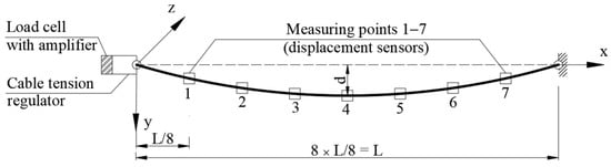
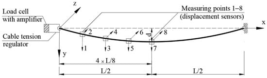
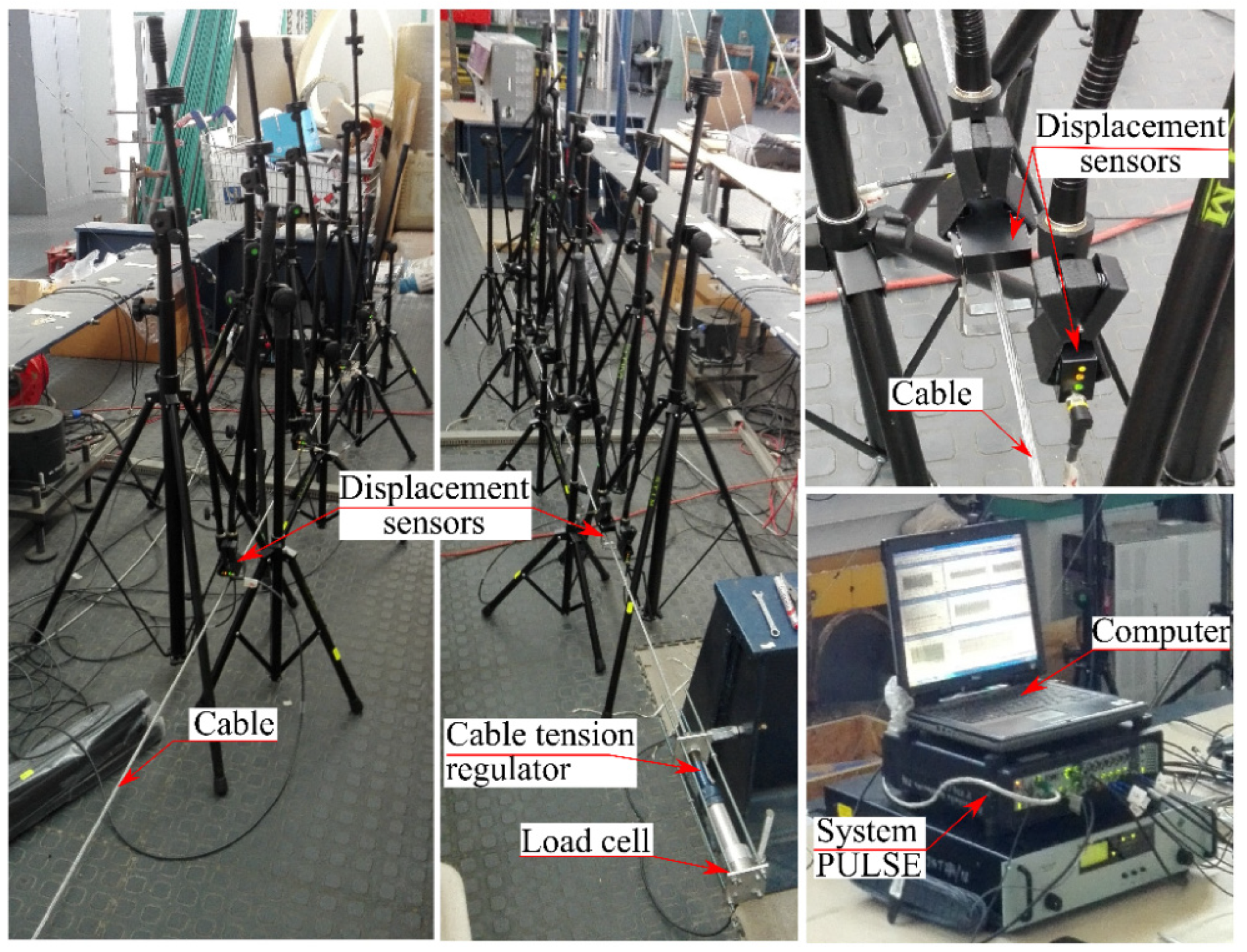
The experimental study was conducted on a cable with the geometric and material parameters summarized in Table 1. A schematic diagram of the tested cable is shown in Figure 1, Figure 2 and Figure 3. The cable span was defined as the horizontal distance between supports positioned at the same elevation. At one end, the cable was secured to the support using a manual tension adjustment mechanism. At the opposite end, the cable was mounted to the support via an eye-sling, creating a pinned support condition (Figure 1, Figure 2 and Figure 3).
Table 1.
Cable geometric and material parameters.
Figure 1.
A model of the tested cable—initial sensor setup (measurements along the y-axis).
Figure 2.
A model of the tested cable—second sensor setup (measurements along the y- and z-axes).
Figure 3.
Experimental test stand and equipment used in the study.
The tests were performed using two different sensor layout configurations along the cable. In the first arrangement, seven displacement sensors were used for non-contact vibration measurements, placed at regular intervals of L/8 along the entire length of the cable (Figure 1).
In the second arrangement, eight displacement sensors were used for non-contact vibration measurement. Four of these sensors (odd-numbered: 1, 3, 5, 7) measured displacements within the cable’s sag plane (along the y-axis), while the remaining four (even-numbered: 2, 4, 6, 8) recorded out-of-plane displacements (along the z-axis). The sensors were arranged over half of the cable length at equal intervals of L/8 (Figure 2).
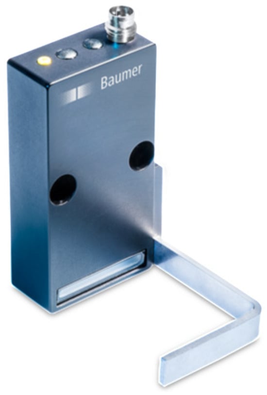
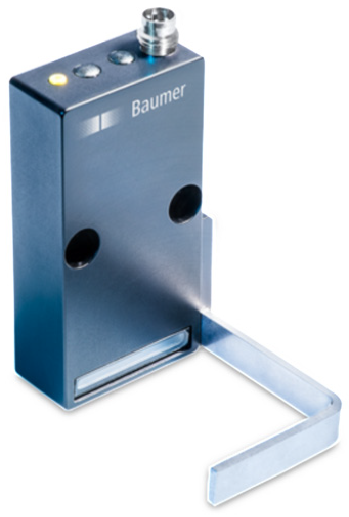
Non-contact vibration measurements were performed using Baumer ZADM 034 displacement sensors (Baumer GmbH, Frauenfeld, Switzerland) (Figure 4). The main specifications of the sensors include measuring range of 24 mm, a working distance to the object of 0 to 40 mm, resolution below 0.05 mm, and minimum detectable object size: 1 mm. The sensors were spaced at equal intervals of L/8 between the supports (Figure 1, Figure 2 and Figure 3).
Figure 4.
A displacement sensor (ZADM 034 Baumer, Baumer GmbH, Frauenfeld, Switzerland).
3. Natural Frequencies and Modal Shapes—Theoretical Background
To determine the cable tension force, the well-known relationships proposed by Irvine and Caughey [1] and Irvine [2] for a cable model with small sag (0 ≤ d/L ≤ 1/8) were employed. In the following equations, the notation is defined as follows: L—cable span defined as the horizontal distance between supports located at the same elevation, m—cable mass per unit length, A—cross-sectional area, H—tension force, E—Young’s modulus, g—gravitational acceleration, and d—cable sag at mid-span. The angular frequency of natural vibrations ω is related to the natural frequency f by the equation ω = 2π f.
3.1. In the Cable Sag Plane—Antisymmetric Mode Shapes (Even Mode Numbers)
The antisymmetric mode shape of an even number 2i is described by the following relationship:
where A2i is a constant vibration amplitude. The corresponding natural circular frequency ω2i is expressed by the following formula:
3.2. In the Cable Sag Plane—Symmetric Mode Shapes (Odd Mode Numbers)
The symmetric mode shape of an odd number 2i − 1 is described by the following relationship:
where A2i−1 is a constant amplitude, while is a dimensionless frequency determined from the transcendental equation:
The dimensionless frequency is related to the i-th natural frequency of the cable ω2i−1 for symmetric in-plane vibrations by the following relationship:
Irvine’s parameter λ2 is defined as [1,2]:
Assuming a static small sag of parabolic shape, d can be expressed as follows:
Equation (3) describes symmetric mode shapes in the case of a significant value of Irvine’s parameter λ2. Conversely, for small values of λ2 (when the effect of axial flexibility and sag on symmetric vibrations is negligible), the analytical expressions describing symmetric mode shapes and their corresponding frequencies in the sag plane reduce to a form identical to that of the antisymmetric modes [1,2]:
3.3. Out of the Cable Sag Plane—Symmetric and Antisymmetric Mode Shapes
Symmetric and antisymmetric out-of-plane mode shapes (transverse/lateral vibrations) and their corresponding natural frequencies are expressed by the following:
In the classical taut string problem—i.e., for a cable model with negligibly small sag—the natural mode shapes and frequencies, both in-plane and out-of-plane, are described by the universal relationships (10) and (11).
4. Experimental and Numerical Studies
4.1. Description of the Method for Determining the Cable Force
The cable tension force was identified using the following procedure:
- Tension Application: A target force was applied to the cable using a manual tension-adjustment mechanism.
- Vibration Signal Acquisition: Cable displacements were recorded using the measuring system under two sensor configurations:
- First setup: One-dimensional measurements restricted to the cable’s sag plane (y-axis).
- Second setup: Two-dimensional measurements recorded simultaneously in the sag plane (y-axis) and out of the sag plane (z-axis).
- Operational Modal Analysis: The recorded displacement signals were processed using Operational Modal Analysis (OMA) to identify the experimental natural frequencies and mode shapes.
- Modal Parameter Comparison: The experimental modal parameters (natural frequencies and mode shapes) were compared with the corresponding analytical results obtained from Equations (1)–(11).
- Cable Tension Force Identification: The cable tension force H was identified by minimizing the relative error () between the experimental (fe,i) and theoretical (fc,i) natural frequencies calculated using Irvine’s analytical Equations (1)–(11):
The identified experimental mode shapes were additionally verified against the analytical spatial distributions to ensure correct mode classification, particularly near the frequency crossover region where the symmetric and antisymmetric modes become closely spaced.
The practical implementation of steps 2 and 3, concerning dynamic data acquisition and signal processing, is described in detail below.
Dynamic signals were acquired using a multi-channel Brüel & Kjær measurement system PULSE LabShop version 21.0.0.671 (Brüel & Kjær, Nærum, Denmark), integrated with Operational Modal Analysis (OMA) via the ARTeMIS Modal software suite version 5.4. The recorded displacements exhibited characteristics of ambient and free vibrations with very small amplitudes ranging from 0.03 mm to 0.06 mm, confirming the high sensitivity of the applied Baumer ZADM 034 non-contact laser sensors.
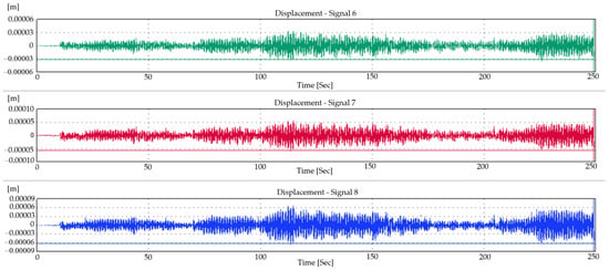
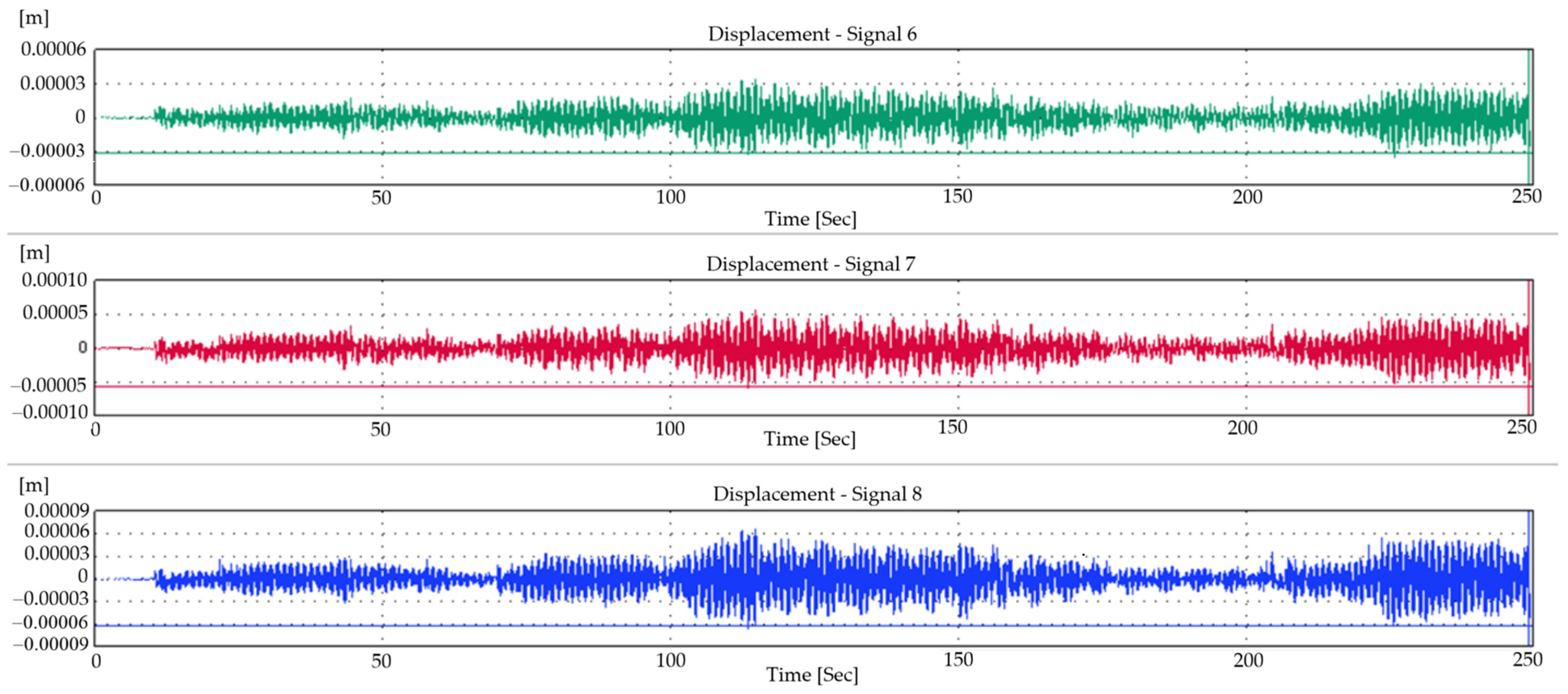
During the experimental tests, signals recorded over various durations (between 1 and 5 min) were analyzed to evaluate the stability of the obtained modal parameters. Measurements were carried out at sampling frequencies fs = 256 Hz and 512 Hz, with corresponding frequency analysis bands (frequency spans up to 100 Hz or 200 Hz). Figure 5 illustrates representative time histories of displacements from a recorded test with a duration of 250 s. For readability and due to the large volume of collected data, detailed presentations of all time histories are omitted in the remainder of this paper in favor of summarizing the final modal analysis results.
Figure 5.
Representative displacement time histories recorded by selected sensors.
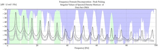
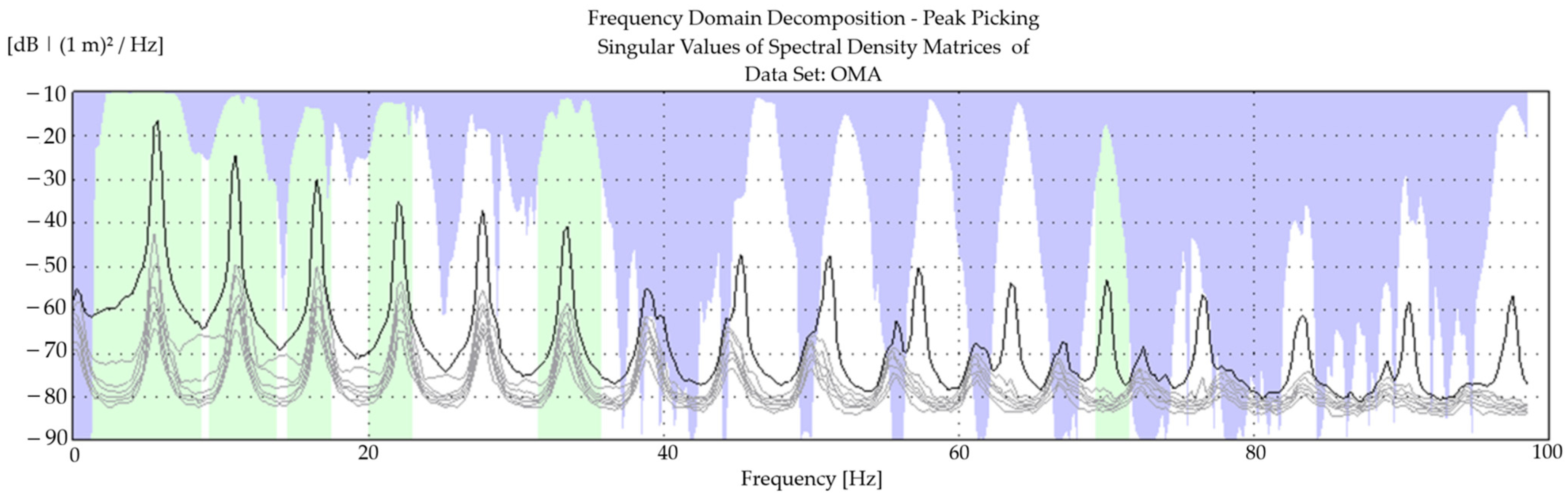
The Frequency Domain Decomposition (FDD) algorithm (often referred to as Peak Picking) was utilized for modal parameter identification. Additionally, signal decimation to lower cutoff frequencies (e.g., 10 Hz and 25 Hz) was applied during the post-processing stage. This filter removed higher-frequency noise components, allowing for a precise determination of the natural frequencies and mode shapes. Figure 6 presents a representative singular value plot of the spectral density matrix obtained in the ARTeMIS Modal software package, showing clearly defined peaks corresponding to successive natural frequencies.
Figure 6.
Singular values of the spectral density matrix with natural frequency identification using the FDD method in ARTeMIS Modal software (B&K PULSE system).
4.2. Estimation of Cable Tension—First Sensor Setup
In this initial configuration, the natural frequencies were identified based on representative single-run measurements to validate the baseline theoretical model. A comprehensive statistical analysis—incorporating repeated measurement series, sample means, standard deviations, and coefficients of variation—is subsequently presented in Section 4.3 for the second sensor setup.
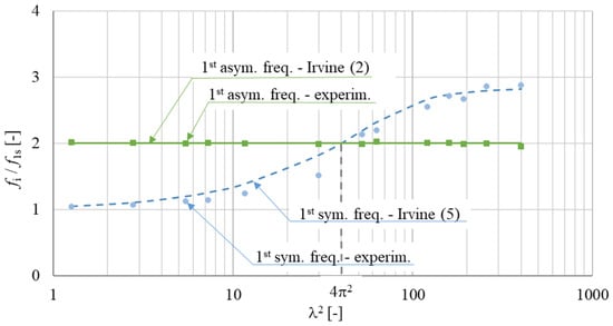
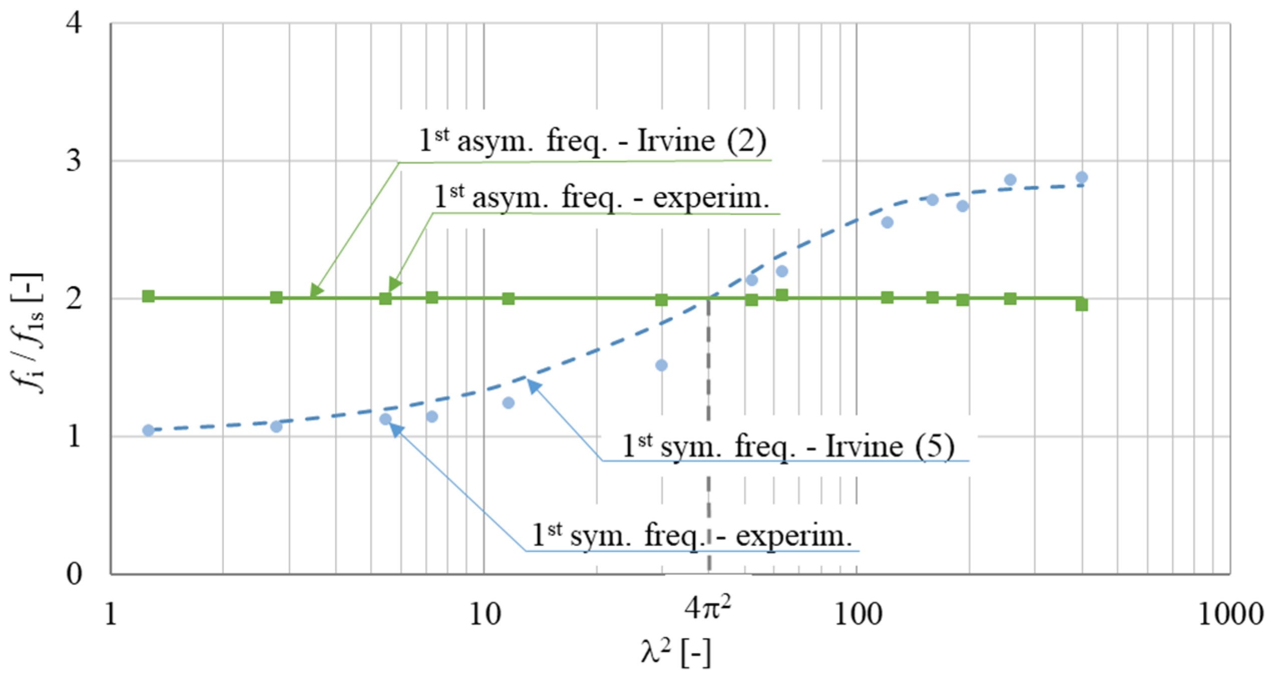
Table 2 and Figure 7 summarize the results for the first symmetric and first antisymmetric modes obtained from experimental testing (OMA) and analytical calculations as a function of the Irvine parameter λ2 (Equation (6)). The analytical calculations were carried out using the cable model proposed by Irvine—Equations (2) and (5)—and the classical taut string model—Equation (11).
Table 2.
Comparison between experimental and numerical results.
Figure 7.
Comparison of natural frequencies. Numerical results: --- 1st symmetric frequency, — 1st antisymmetric frequency. Experimental results: ● 1st symmetric frequency, ■ 1st antisymmetric frequency.
Figure 7 shows the first two natural frequencies, corresponding to the first symmetric and first antisymmetric mode shapes, normalized with respect to the fundamental natural frequency of the taut string (Equation (11)). In this manner, normalized (dimensionless) frequency values were obtained.
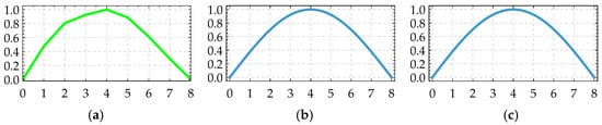
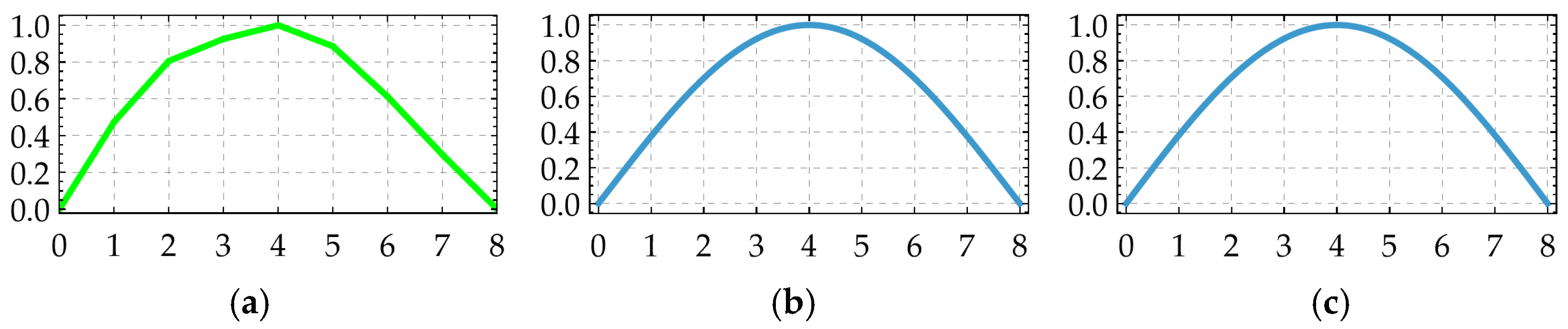
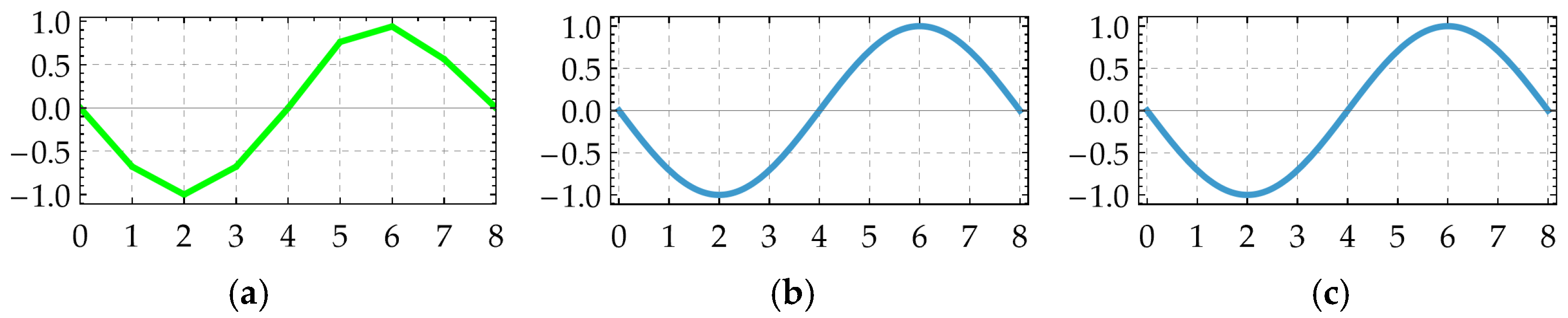
The first symmetric and antisymmetric mode shapes for three representative tests are shown in Figure 8, Figure 9, Figure 10, Figure 11, Figure 12 and Figure 13. These results were obtained from displacement signals recorded along the vertical direction (sag plane, y-axis). The mode shapes presented in Figure 8 and Figure 9 represent the case of a low Irvine parameter value (λ2 = 1.3). In contrast, the plots in Figure 10, Figure 11, Figure 12 and Figure 13 relate to higher values of this parameter, namely λ2 = 62.9 (Figure 10 and Figure 11) and λ2 = 121.3 (Figure 12 and Figure 13), respectively.
Figure 8.
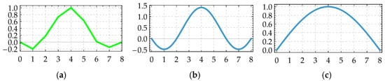
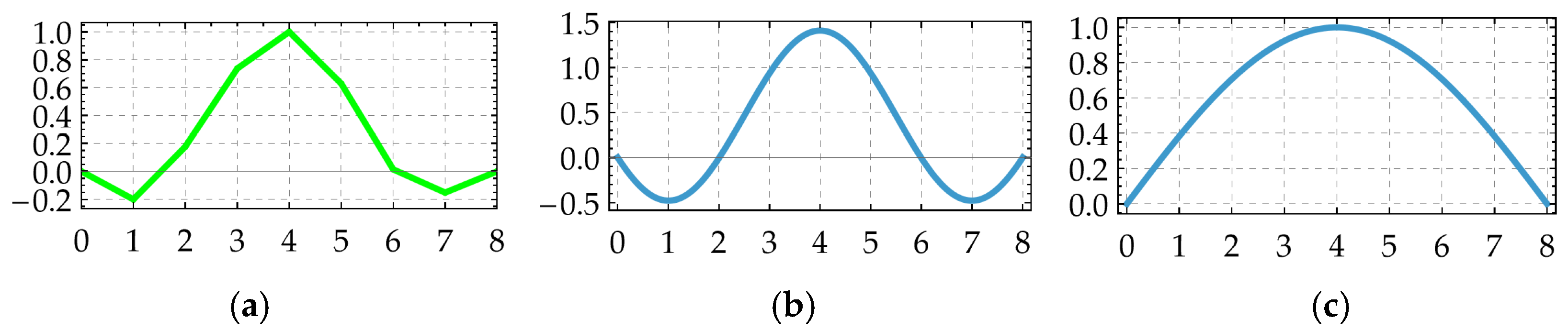
Mode shapes corresponding to the first natural frequency for tension force H = 398.1 N, λ2 = 1.3: (a) experimental results fe1 = 5.67 Hz, (b) Irvine formulas fI1 = 5.73 Hz, (c) string formulas fs1 = 5.46 Hz.
Figure 9.
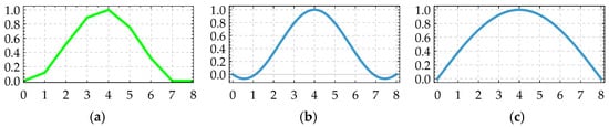
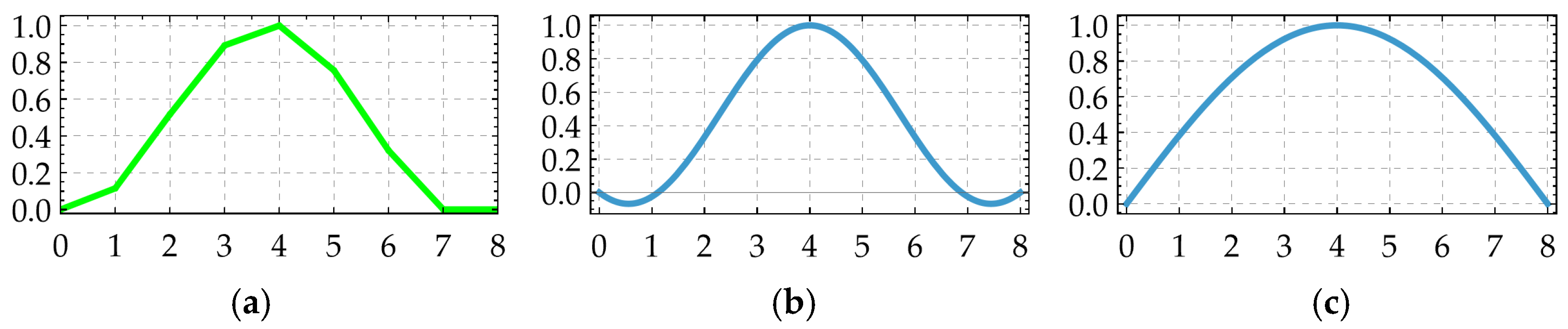
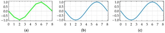
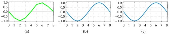
Mode shapes corresponding to the second natural frequency for tension force H = 398.1 N, λ2 = 1.3: (a) experimental results fe2 = 10.99 Hz, (b) Irvine formulas fI2 = 10.92 Hz, (c) string formulas fs2 = 10.92 Hz.
Figure 10.
Mode shapes corresponding to the first natural frequency for tension force H = 108.2 N, λ2 = 62.9: (a) experimental results fe1 = 6.25 Hz, (b) Irvine formulas fI1 = 6.61 Hz, (c) string formulas fs1 = 2.85 Hz.
Figure 11.
Mode shapes corresponding to the second natural frequency for tension force H = 108.2 N, λ2 = 62.9: (a) experimental results fe2 = 5.77 Hz, (b) Irvine formulas fI2 = 5.69 Hz, (c) string formulas fs2 = 5.69 Hz.
Figure 12.
Mode shapes corresponding to the first natural frequency for tension force H = 86.9 N, λ2 = 121.3: (a) experimental results fe1 = 6.61 Hz, (b) Irvine formulas fI1 = 6.68 Hz, (c) string formulas fs1 = 2.44 Hz.
Figure 13.
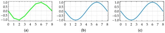
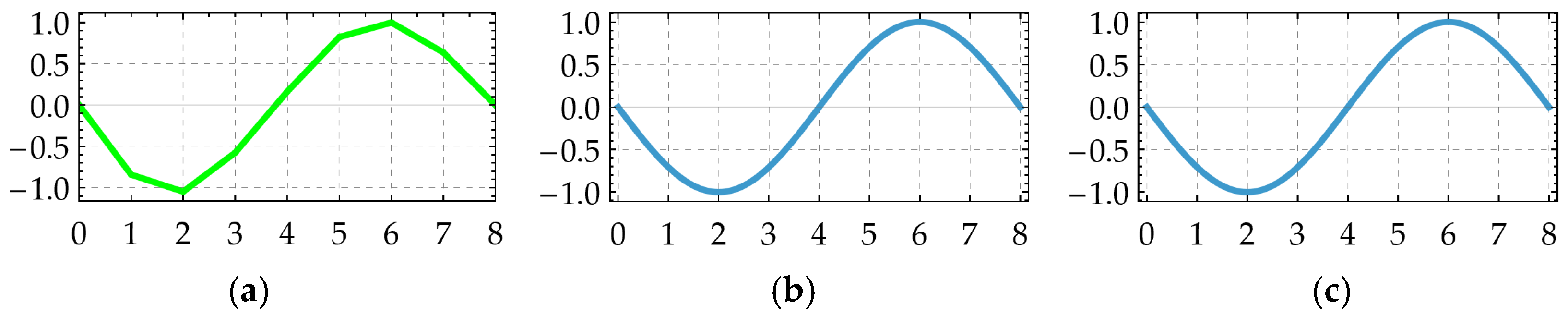
Mode shapes corresponding to the second natural frequency for tension force H = 86.9 N, λ2 = 121.3: (a) experimental results fe2 = 4.87 Hz, (b) Irvine formulas fI2 = 4.87 Hz, (c) string formulas fs2 = 4.87 Hz.
The mode shape profiles obtained from experimental measurements demonstrate a high degree of agreement with the theoretical results based on the small-sag cable model. Remarkably, for large values of the parameter λ2, the first symmetric mode shape exhibits a characteristic profile with three local extrema (Figure 10a,b and Figure 12a,b). According to the theory, this mode features a single local extremum for λ2 < 4π2, whereas exceeding the threshold λ2 > 4π2 results in the appearance of three such extrema.
Under the condition λ2 > 4π2, a crossover in the sequence of mode shapes also occurs—the frequency of the first symmetric vibration mode exceeds that corresponding to the first antisymmetric mode. This phenomenon is illustrated by the measurement results for λ2 = 62.9, where fe2 = 5.77 Hz was recorded for the first antisymmetric mode (Figure 11a), while the first symmetric mode reached a higher value of fe1 = 6.25 Hz (Figure 10a; a difference of approx. 8%). An analogous frequency crossover was also observed for the test with the lowest tension force H = 86.9 N (λ2 = 121.3), yielding fe2 = 4.87 Hz (Figure 13a) and fe1 = 6.607 Hz (Figure 12a).
As the parameter λ2 approaches the critical value of 4π2, the frequencies of the symmetric and antisymmetric modes become very close to each other. Under such conditions, frequency measurements alone may be insufficient for reliable cable force estimation, as the identified frequencies may be difficult to assign unambiguously to the corresponding modal branches. The application of OMA, which provides both natural frequencies and associated mode shapes, enables the correct identification and ordering of the modes and therefore supports reliable cable force estimation.
Furthermore, the frequency crossover observed near λ2 ≈ 4π2 has a clear mechanical interpretation. Within the Irvine–Caughey formulation, this phenomenon results from the linearized mechanical coupling between transverse in-plane motion, cable geometry, and axial extensibility. This coupling is particularly important for in-plane symmetric modes, where transverse deformation is accompanied by changes in cable length and, consequently, variations in axial force. In contrast, the antisymmetric modes involve a different deformation symmetry, which substantially reduces the associated net change in cable length and, consequently, the contribution of axial-force variation to their dynamic response. The dynamic response of these modes depends not only on the geometric stiffness associated with initial tension and sag but also on the stiffness contribution from axial extensibility.
For λ2 < 4π2, the first in-plane symmetric mode is characterized by a deformation profile without internal nodes and a specific balance between geometric and axial stiffness contributions. As λ2 increases, the relative influence of these two mechanisms evolves, progressively altering both the natural frequencies and the associated mode shapes. When λ2 approaches the critical value of 4π2, the interaction between these stiffness components becomes critical, causing the frequencies of the first symmetric and first antisymmetric modes to converge until they coincide at λ2 = 4π2. Beyond this threshold, the modal ordering interchanges: the first symmetric frequency exceeds the first antisymmetric frequency. Simultaneously, the first symmetric mode undergoes a qualitative change in its modal shape, manifested by the appearance of two internal nodes and three local extrema.
Thus, the frequency crossover should not be regarded merely as a mathematical feature of the Irvine formulation. It is a manifestation of the mechanical interaction between cable geometry, initial tension, axial deformation, and transverse vibration. This mechanism is particularly important for vibration-based cable force identification. Neglecting cable sag and axial extensibility leads to a simplified model that mispredicts the modal ordering. This, in turn, can cause incorrect mode identification during experimental data assignment and lead to erroneous estimates of the cable tension force.
Comparing the natural frequency values and mode shapes obtained from the experimental tests with the analytical results therefore allows the cable tension force to be efficiently and accurately determined using the proposed methodology. The cable force for each test was identified by minimizing the differences between the measured and calculated values of the first two natural frequencies and by maximizing the agreement between their corresponding mode shapes. The tension forces estimated for the individual tests are summarized and compared in Table 2.
4.3. Estimation of Cable Tension—Second Sensor Setup
4.3.1. Test Configuration and Statistical Framework
In the second sensor setup (Figure 2), three test trials were conducted for three target cable tension forces: H1, H2, and H3. Although displacements were recorded simultaneously in two directions (y and z) in this variant, two signal processing approaches were analyzed to perform a comparative study and demonstrate the differences in the results. For the natural frequencies corresponding to out-of-plane mode shapes, both two-dimensional (yz) signals and one-dimensional signals restricted solely to the z-axis (omitting the y-direction) were analyzed. Similarly, when determining the frequencies for symmetric in-plane modes, results obtained from the full set of signals (yz) were compared with those based only on the four signals along the y-axis (omitting the z-axis).
To comprehensively address the statistical repeatability of individual trials across the measurement series, detailed statistical parameters are presented specifically for a representative tension force H1 ≈ 221 N. For the remaining tension levels (H2, and H3), the mean experimental natural frequencies are utilized to illustrate global frequency–tension trends without unnecessarily expanding the tabular data.
4.3.2. Modal Identification and Experimental Mode Shapes
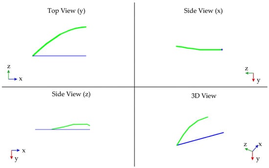
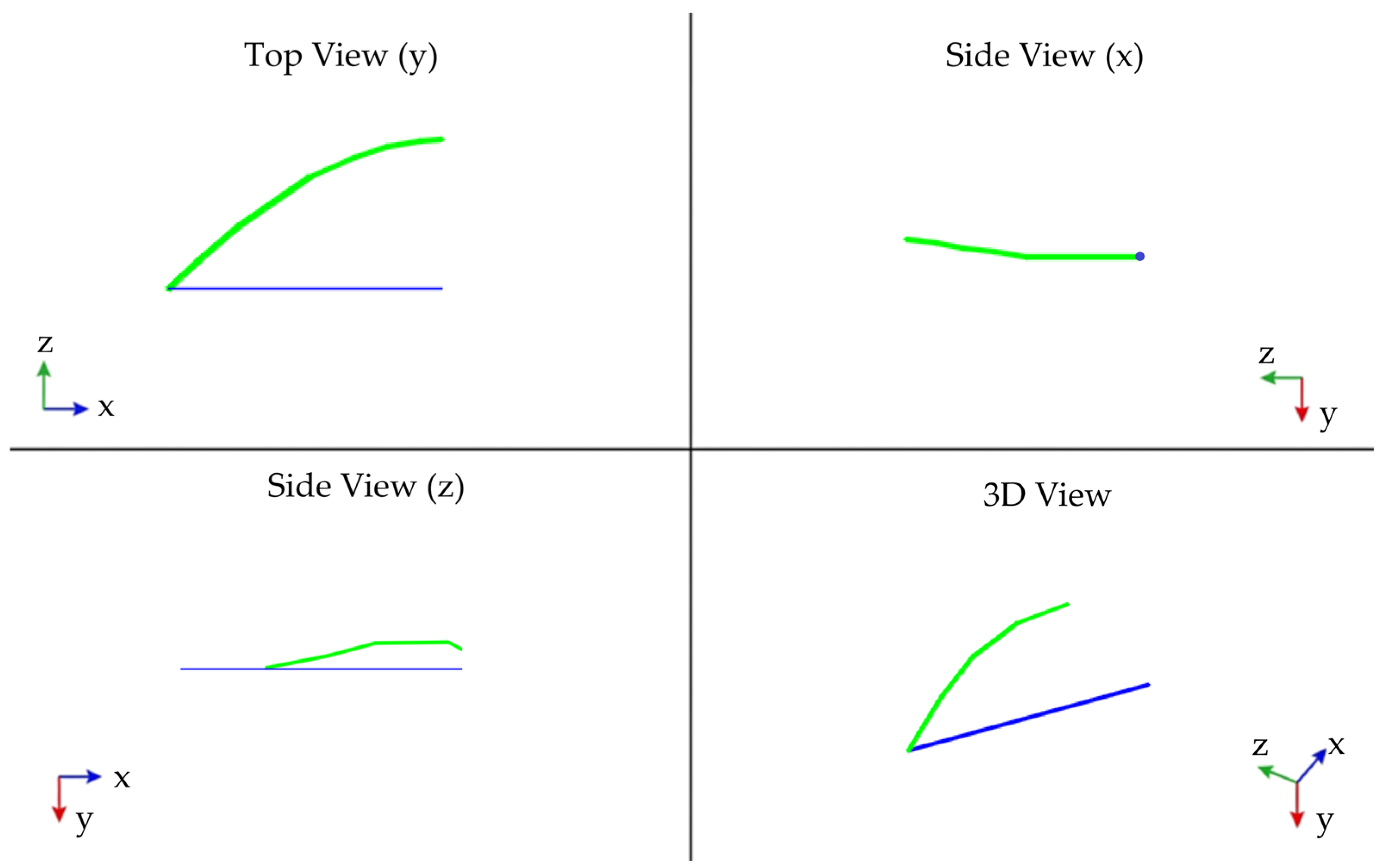
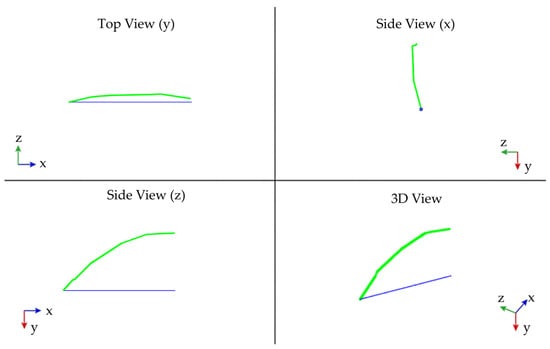
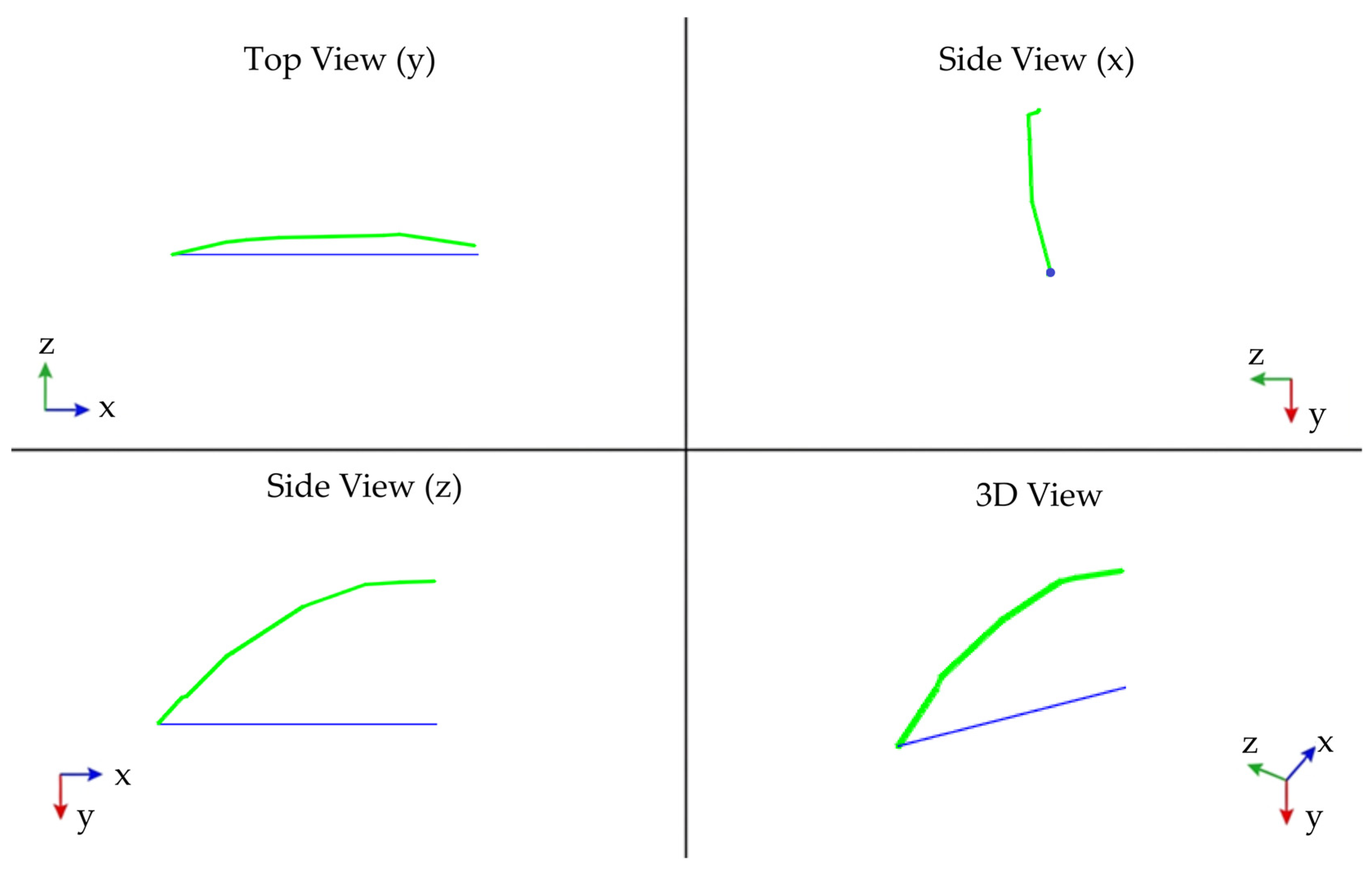
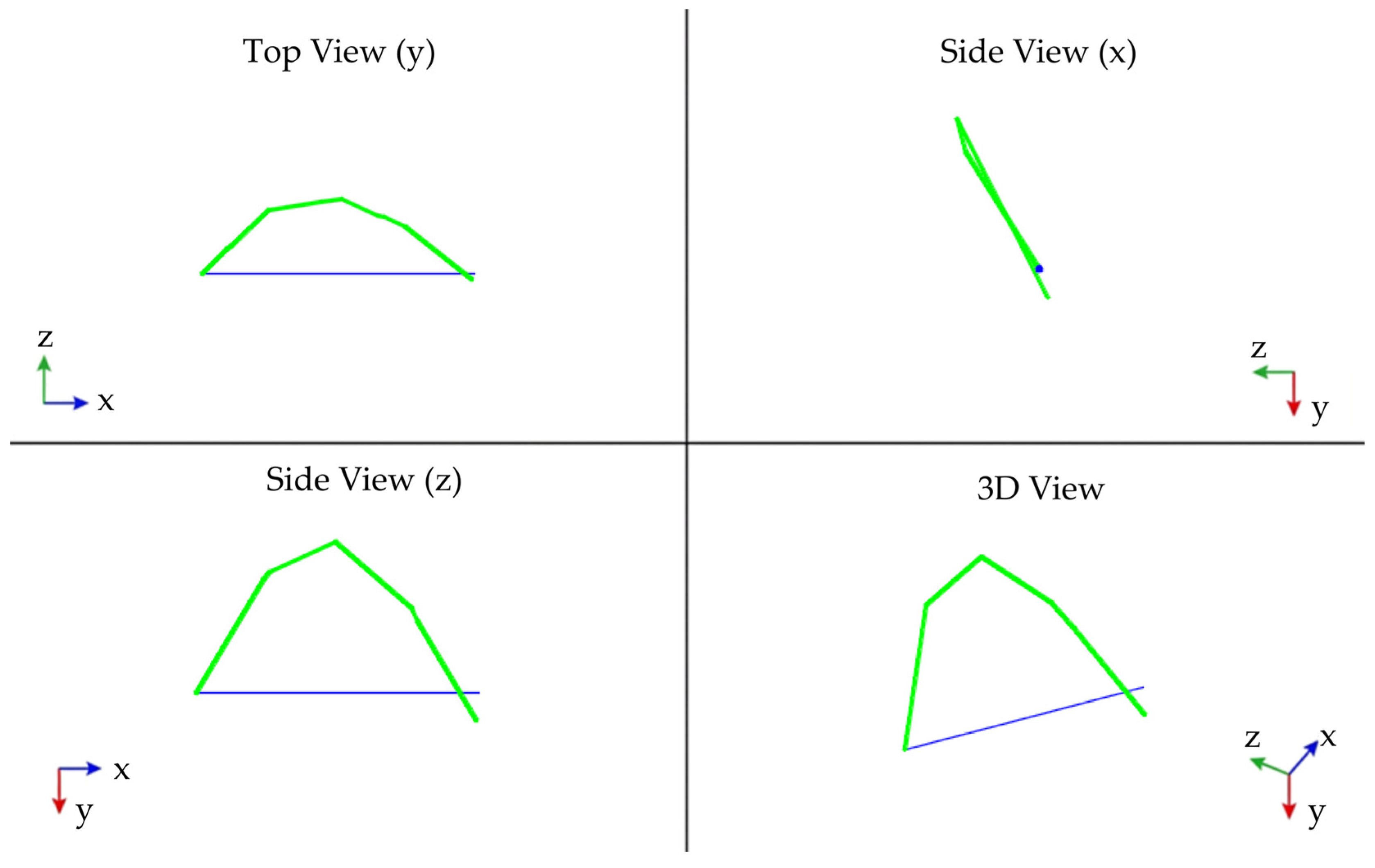
Figure 14, Figure 15 and Figure 16 present exemplary natural mode shapes obtained from experimental testing (OMA) for selected measurements conducted using eight sensors measuring displacements two-dimensionally (four sensors along the y-axis and four along the z-axis, positioned on one side of the cable). The presented mode shapes correspond to an identified cable tension force of H1 ≈ 221 N.
Figure 14.
Experimental results (OMA) for a selected measurement trial (H1 ≈ 221 N). First out-of-plane symmetric mode shape corresponding to a natural frequency of 3.95 Hz.
Figure 15.
Experimental results (OMA) for a selected measurement trial (H1 ≈ 221 N). First in-plane symmetric mode shape corresponding to a natural frequency of 4.60 Hz (first Irvine mode).
Figure 16.
Experimental results (OMA) for a selected measurement trial (H1 ≈ 221 N). First in-plane and out-of-plane antisymmetric mode shape corresponding to a natural frequency of 8.10 Hz.
Figure 14 presents the first out-of-plane symmetric mode shape corresponding to a natural frequency of 3.95 Hz, showing distinct, dominant displacements in the z-axis.
Figure 15 shows the first in-plane symmetric mode shape for a natural frequency of 4.60 Hz (the so-called “first Irvine frequency”), characterized by dominant displacements along the y-axis.
In turn, Figure 16 presents the first antisymmetric natural mode shape of the cable corresponding to a natural frequency of 8.10 Hz, in which almost identical displacement amplitudes were recorded in both directions (y and z), demonstrating its clear three-dimensional character.
In accordance with the simplified linear vibration theory presented in Section 3, the natural frequency values and their corresponding antisymmetric mode shapes both in-plane and out-of-plane should be identical. However, in selected measurement series, the antisymmetric mode shapes exhibited a distinct character—clearly dominant displacements were observed along either the y-axis or the z-axis. This situation can be attributed to the influence of real-world physical factors, such as imperfectly hinged cable end supports, unintended initial excitation disturbances, local asymmetry in mass distribution, or ambient noise.
The presented identification of mode shapes and their accompanying spatial disturbances confirms that incorporating multidirectional modal analysis is crucial for the correct interpretation of cable behavior. The discussed relationships and observed physical phenomena lead directly to the quantitative tension estimation presented in the following section.
4.3.3. Tension Estimation for Representative Load Case
A comparative quantitative analysis of one-dimensional (y or z) and two-dimensional (yz) signal processing approaches is presented below for the representative tension level H1 ≈ 221 N. The measured natural frequencies, statistical evaluations, estimated individual tension forces Hi, mean identified forces Hmean, and model fitting errors are summarized in Table 3 and Table 4.
Table 3.
Statistical summary of measured out-of-plane natural frequencies and identified cable tension forces for H1 (comparison of yz and z directional analyses).
Table 4.
Statistical summary of measured in-plane natural frequencies and identified cable tension forces for H1 (comparison of yz and y directional analyses).
To rigorously evaluate measurement repeatability, the sample mean frequency from n measurement trials was evaluated alongside key statistical indicators:
- Standard Deviation (SD):
- Standard Error of the Mean (SEM):
- Margin of Error (ME) for the 95% Confidence Interval (95% CI), calculated for the mean natural frequency (expressed as ) using the critical value of Student’s t-distribution () for a significance level and n − 1 degrees of freedom due to the limited sample size (n < 30):
- Coefficient of Variation (CV): Expressing relative dispersion to confirm test-setup stability:
All calculated CV values remain well below 5% (max. 1.82% for out-of-plane and 1.49% for in-plane tests), indicating the high measurement stability and repeatability across the individual trials.
Table 3 compiles the measured out-of-plane natural frequencies and identified cable tension forces, comparing the two-dimensional (yz) analysis with the one-dimensional (z-axis) analysis.
Table 4 summarizes the measured in-plane symmetric natural frequencies and corresponding tension forces, comparing two-dimensional (yz) signals with one-dimensional (y-axis) signals.
It should be emphasized that the first in-plane symmetric frequency, for which the relative discrepancy reaches −10.1%, was not used directly for the estimating cable tension. As indicated in Table 4, no individual force Hi was determined from this frequency. Instead, the first symmetric mode shape was retained for modal identification, allowing the corresponding frequency to be correctly associated with the first symmetric mode and distinguished from the first antisymmetric mode. The tension force was determined from the higher-order modes (modes 3 and 5), for which substantially better agreement between the experimental and analytical frequencies was achieved.
Analyzing the obtained results, good agreement can be observed between the force values determined independently from one-dimensional in-plane (y-axis) and out-of-plane (z-axis) vibrations. For the representative test H1, the estimated values (H1 = 221.91 N for z-axis measurements and H1 = 221.75 N for y-axis measurements, with Irvine parameter λ2 = 7.30) differ slightly, by only about 0.07%:
Taking the detailed data from trial H1 as an example (Table 3 and Table 4), it was also demonstrated that using a two-dimensional (yz) analysis leads to slightly lower tension force values compared to the one-dimensional analysis. The relative differences are as follows:
- For out-of-plane vibrations (z-axis vs. yz):
- For in-plane vibrations (y-axis vs. yz):
This slight reduction confirms that incorporating spatial (yz) interaction avoids minor overestimations of the system stiffness that occur when restricting modal analysis to purely single-axis displacement signals.
4.3.4. Global Frequency–Tension Relationships Across Load Levels
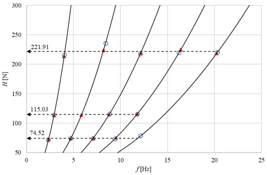
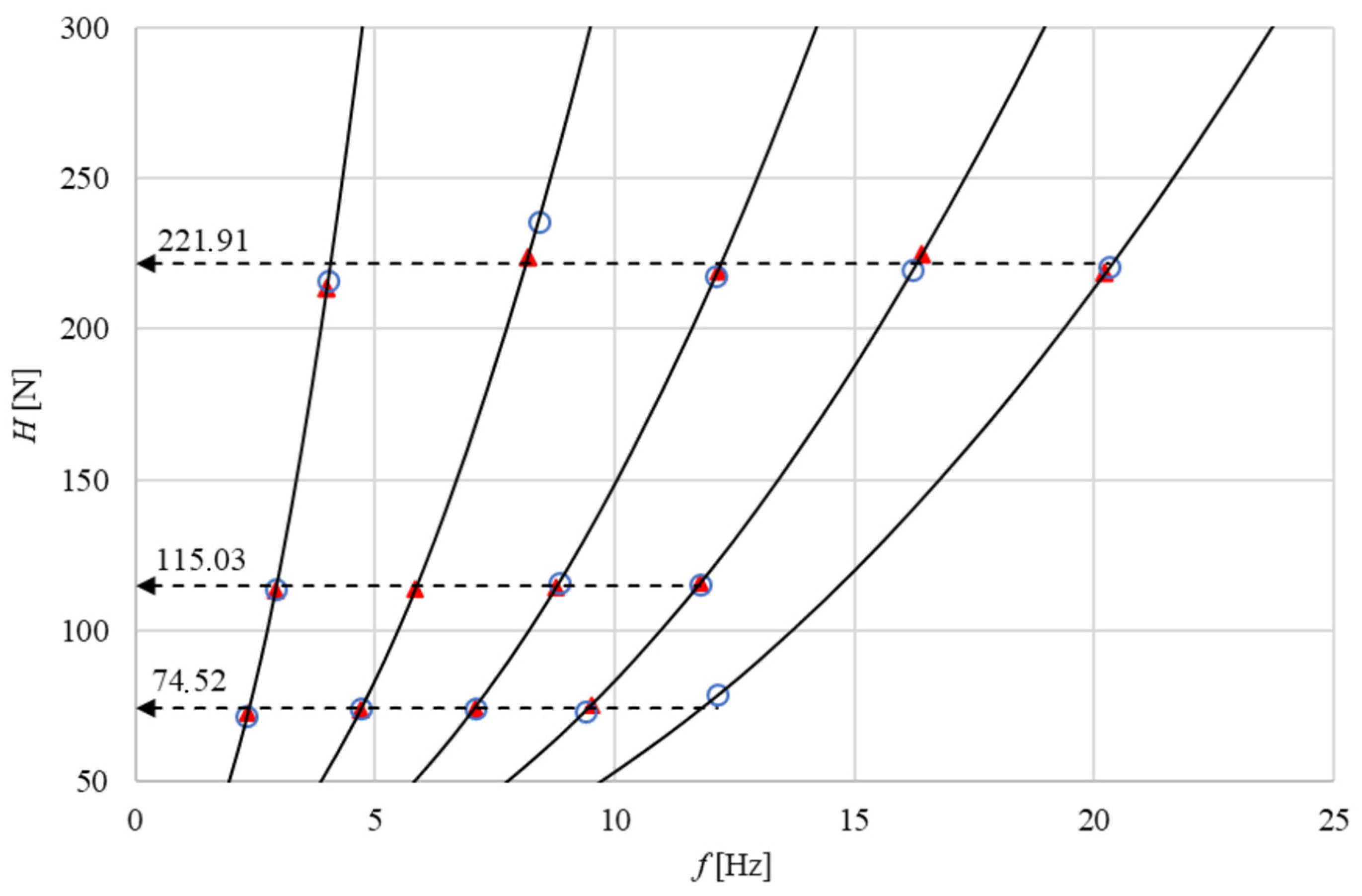
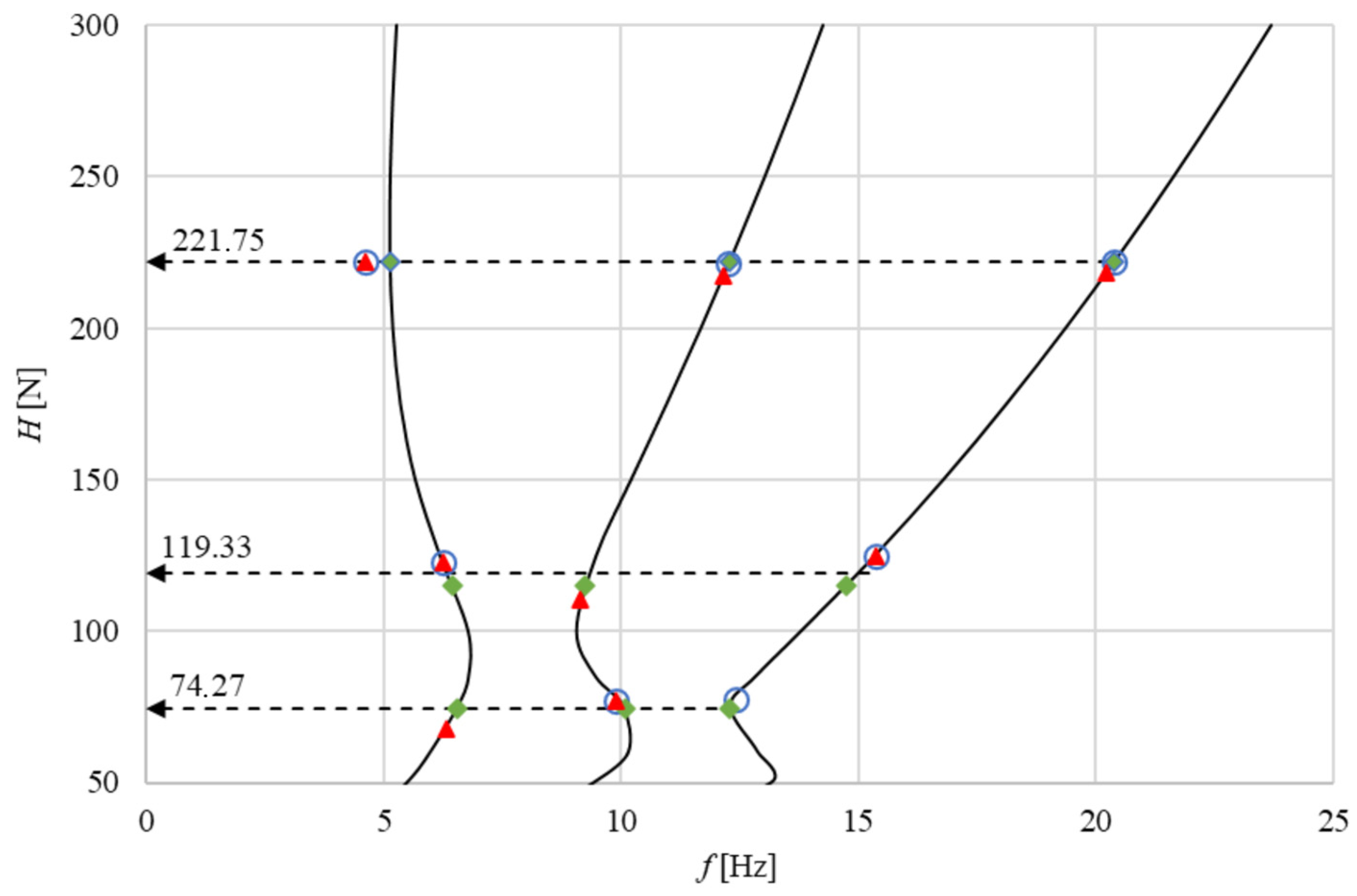
To evaluate the cable behavior across a broader operating tension range, the overall frequency-versus-tension relationships for all three investigated force levels (H1 ≈ 221 N, H2 ≈ 115 N, and H3 ≈ 74 N) are illustrated graphically in Figure 17 and Figure 18.
Figure 17.
The first five out-of-plane natural frequencies f in relation to the cable tension force H. Natural frequencies: — calculated; ○ determined from signals measured along the z-axis; ▲ determined from signals measured along both y- and z-axes.
Figure 18.
The first three in-plane symmetric natural frequencies f in relation to the cable tension force H. Natural frequencies: — calculated; ♦ frequencies calculated for the average force values determined from out-of-plane natural frequencies; ○ determined from signals measured along the y-axis; ▲ determined from signals measured along both y- and z-axes.
Figure 17 shows the dependence of the first five natural frequencies (corresponding to out-of-plane vibration modes) on the tension force H. The continuous lines indicate the natural frequencies calculated analytically using Equation (11). The measurement points (marked with circles and triangles) represent the experimental natural frequencies obtained via OMA for individual tension forces (H1, H2, and H3). The red triangles correspond to frequencies determined from eight signals recorded simultaneously in two directions (y and z). In turn, the blue circles represent frequencies calculated from four signals measured exclusively along the z-axis (omitting the y-axis signals). The dashed lines mark the average force values (H1 = 221.91 N, H2 = 115.03 N, H3 = 74.52 N) calculated from Equation (11) using frequencies measured solely in the z-axis direction.
Figure 18 shows the dependence of the first three in-plane symmetric natural frequencies on the tension force H. The continuous lines indicate the natural frequencies calculated analytically based on Equation (5). Red triangles denote the natural frequencies obtained from eight signals measured simultaneously in two directions (y and z). In turn, blue circles represent frequencies determined from four signals measured exclusively along the y-axis (omitting signals from the z-axis direction). The dashed lines mark the average force values (H1 = 221.75 N, H2 = 119.33 N, and H3 = 74.27 N) calculated from Equation (5) using frequencies measured in the y-axis direction. Green diamonds represent natural frequencies calculated from Equation (5) for the average force values previously determined based on out-of-plane cable vibrations (Figure 17).
The characteristic, non-linear course of the frequency branches in Figure 18 results directly from Irvine’s theoretical formulation. For in-plane symmetric vibrations, the natural frequencies are influenced not only by the tension force H but also by changes in geometric stiffness associated with cable sag (described by the parameter λ2). The visible inflections and the change in curve monotonicity correspond to passing through the critical region λ2 ≈ 4π2 (the so-called frequency crossover phenomenon). The good agreement between the experimental OMA results and the analytical curves over most of the investigated range supports the applicability of the adopted theoretical model.
An overall analysis of the plots allows for an evaluation of the cable behavior at lower tension levels (H2 and H3). In the second test, the largest discrepancy between out-of-plane and in-plane vibrations was observed (H2 = 115.03 N vs. H2 = 119.33 N, a difference of 3.60%), which is associated with the proximity to the critical region λ2 ≈ 4π2. Consequently, this may lead to disturbances in frequency and/or mode shape measurements or a misinterpretation of the obtained results (this issue is analyzed in detail in Section 4.2). In this transition regime, where adjacent symmetric and antisymmetric frequencies coalesce, tension identification becomes particularly sensitive to localized spatial mode variations, support compliance, and flexural rigidity effects. Under such conditions, 2D OMA spatial mode shape verification plays a critical role in preventing mode misclassification. Furthermore, increasing spatial sensor density near nodal points and cable boundaries could potentially offer higher spatial resolution to better capture these subtle mode variations in future studies. For the third test, this difference decreases again to just 0.34% (H3 = 74.52 N vs. H3 = 74.27 N).
5. Conclusions
This paper presents a methodology for identifying the tension force in sagged cables with small static sag (0 ≤ d/L ≤ 1/8), using operational modal analysis (OMA) combined with Irvine’s analytical model. The conducted laboratory tests under various sensor configurations demonstrated the effectiveness of OMA for estimating the tension force of cables with significant geometric sag. A very good agreement was achieved between the experimental results and the theoretical model, where the relative errors in force determination for cases located outside the critical region (λ2 < 4π2 or λ2 > 4π2) were only 0.07% (for trial H1) and 0.34% (for trial H3).
Determining not only the natural frequencies but also the mode shapes proved to be crucial in the frequency crossing region (λ2 ≈ 4π2 ≈ 39.5). For trial H2, located in the immediate vicinity of this critical region, a discrepancy of 3.60% was observed. This behavior is associated with the mechanical interaction between geometric stiffness and axial extensibility, which alters the character of the first symmetric mode shape, including the appearance of additional local extrema beyond the threshold. Identifying the mode shapes via OMA prevents their misclassification in this zone, protecting against significantly larger errors in tension estimation.
Regarding trial H1, a relative frequency discrepancy of −10.1% was observed specifically for the first in-plane symmetric mode. This relatively large discrepancy is likely associated with a combination of theoretical approximations and physical characteristics of the experimental system. First, Irvine’s analytical formulation assumes zero flexural rigidity (EI = 0), whereas the physical cable possesses finite bending stiffness (EI > 0). Since the first symmetric mode involves dynamic axial-force variations and transverse deformation, the finite bending stiffness of the physical cable may contribute to a frequency shift that is not captured by the idealized flexible-string model. Second, minor mechanical compliance in the eye-sling support attachments may additionally affect this mode, particularly because of its coupling between transverse deformation, cable-length variation, and axial force. The corresponding axial-force variation is substantially less pronounced for antisymmetric modes because of their deformation symmetry. Finally, the low coefficient of variation obtained for this frequency (0.77% for the two-dimensional analysis; Table 4) indicates that random measurement uncertainty is unlikely to be the primary source of the observed discrepancy.
Crucially, for the H1 case analyzed using the second sensor setup, the first in-plane symmetric frequency, which exhibited a −10.1% discrepancy, was not used directly for numerical tension estimation. As indicated in Table 4, no individual tension force Hi was back-calculated from this frequency. Instead, its identified 2D spatial mode shape was retained for modal identification and for the correct assignment of the identified frequency to the corresponding theoretical modal branch. The estimated tension force was determined from the higher-order modes (modes 3 and 5), which exhibited substantially better agreement with the analytical model. Consequently, the localized discrepancy in the fundamental symmetric frequency does not translate into a corresponding error in the estimated tension force.
Comparing signals measured two-dimensionally (yz) with one-dimensional measurements (y or z) showed that spatial analysis leads to slightly lower tension force values (by approx. 0.8–1.3%). This indicates a slight overestimation of the system’s stiffness when using simplified one-dimensional measurements.
Furthermore, the statistical analysis performed across repeated measurement series confirmed high experimental stability and measurement repeatability. The calculated coefficients of variation (CV) for the identified natural frequencies remained consistently low (below 1.82% for out-of-plane and 1.49% for in-plane tests), demonstrating that the observed differences in identified frequencies and estimated tension forces are statistically sound and exceed the inherent measurement scatter.
The application of a two-dimensional sensor setup eliminated the problem of modal spectrum incompleteness. During one-dimensional measurements, spatial limitations made it impossible to determine certain natural frequencies and mode shapes (including the second in-plane mode shape for force H2 and the first mode shape for force H3), whereas simultaneous recording in two directions (yz) guaranteed full and reliable system identification.
The analysis of antisymmetric mode shapes for two-dimensional signals confirmed their spatial character, with nearly identical displacement amplitudes in the in-plane (y) and out-of-plane (z) directions. The local dominance of one direction observed in selected trials may result from real-world factors, including non-ideal boundary conditions associated with the manual tension adjustment mechanism and eye-sling attachments, slight asymmetry in mass distribution, or differences in the initial excitation. From a structural dynamics perspective, the influence of local boundary flexibility generally becomes less pronounced as the cable length and slenderness increase. In the present study, the identified mode shapes exhibited nearly sinusoidal profiles, which is consistent with the assumed pinned–pinned analytical model and suggests that any influence of the actual boundary configuration on the measured global dynamic response was small. This interpretation is further supported by previous theoretical findings by the author [52], which showed that discrete elements, elastic constraints, or attached masses located close to the boundaries do not noticeably affect the fundamental natural frequencies under the investigated conditions. Moreover, the good agreement between the experimentally identified frequencies and those obtained from the analytical model, together with the consistency of the identified mode shapes, provides additional evidence that possible deviations from the idealized boundary conditions did not introduce a significant bias into the cable tension estimation in the present study.
Nevertheless, the influence of non-ideal boundary conditions cannot be assumed to be universally negligible, particularly for short or relatively stiff cables, for which local support flexibility may have a more pronounced effect on the measured response. This issue has been addressed in the literature using boundary-independent iterative schemes [44] and unified correction formulas [19,21]. A detailed experimental characterization of the near-support strain and displacement fields was beyond the scope of the present study. Future investigations could therefore employ denser sensor arrays in the vicinity of the supports to quantify local mode-shape distortions and support compliance more directly.
An important limitation of the present study is that the cable was considered in a horizontal configuration; therefore, the influence of the cable inclination angle, which may be relevant in practical cable-supported structures, was not investigated. In addition, the analytical model assumes negligible bending stiffness of the cable and does not systematically account for the influence of concentrated masses and local attachments on tension identification. It should be noted, however, that the measurements were performed using a non-contact optical technique, and no accelerometers or other measurement devices were attached to the cable. Thus, the measurement procedure did not introduce additional concentrated masses or mechanical interference into the investigated system, which is an important advantage for dynamic cable testing and helps to avoid measurement-induced alterations of the cable response and tension identification. Although the influence of non-ideal boundary conditions and attached elements is discussed above, their systematic experimental assessment remains an area for further research. Future engineering-oriented studies should therefore consider inclined cables with different sag-to-span ratios, bending stiffness, and realistic configurations including clamps, dampers, and other attached components. Such investigations could provide practical correction factors or extended identification procedures applicable to in situ cable monitoring under non-ideal structural conditions.
Based on the presented analytical and experimental findings, it can be concluded that the identification of the first symmetric and first antisymmetric modes, together with their corresponding 2D mode shapes, provides sufficient information for reliable modal interpretation and tension estimation for the investigated cable configuration, within the parameter ranges and small static sag conditions considered in this study. The first symmetric mode is particularly important for the correct modal ordering, whereas its frequency may not necessarily be suitable for direct tension estimation when substantial model–experiment discrepancies occur. In such cases, higher-order modes exhibiting better agreement with the analytical model can be used for estimating cable tension. However, cables exhibiting significant flexural rigidity, complex boundary conditions, or large sag-to-span ratios beyond those investigated in this study may still require the inclusion of additional higher modes or a finer sensor grid. Overall, the proposed 2D OMA framework provides an effective and practical balance between experimental setup complexity and force identification accuracy.
Author Contributions
Conceptualization, W.P.; methodology, W.P. and J.G.; software, W.P. and J.G.; validation, W.P. and J.G.; formal analysis, W.P. and J.G.; investigation, W.P. and J.G.; resources, W.P. and J.G.; data curation, W.P. and J.G.; writing—original draft preparation, W.P.; writing—review and editing, W.P. and J.G.; visualization, W.P. and J.G.; supervision, W.P.; project administration, W.P. All authors have read and agreed to the published version of the manuscript.
Funding
This research received no external funding.
Institutional Review Board Statement
Not applicable.
Informed Consent Statement
Not applicable.
Data Availability Statement
The original contributions presented in this study are included in the article. Further inquiries can be directed to the corresponding author.
Conflicts of Interest
The authors declare no conflicts of interest.
Abbreviations
The following abbreviations are used in this manuscript:
| FEM | Finite Element Method |
| FDD | Frequency Domain Decomposition |
| OMA | Operational Modal Analysis |
| SD | Standard Deviation |
| SEM | Standard Error of the Mean |
| ME | Margin of Error |
| CV | Coefficient of Variation |
Appendix A
Table A1.
Measured (in yz-direction) values of out-of-plane natural frequencies.
Table A2.
Measured (in z-direction) values of out-of-plane natural frequencies.
Table A3.
Measured (in yz-direction) values of in-plane natural frequencies.
Table A4.
Measured (in y-direction) values of in-plane natural frequencies.
References
- Irvine, H.M.; Caughey, T.K. The linear theory of free vibrations of a suspended cable. Proc. R. Soc. Lond. A Math. Phys. Sci. 1974, 341, 299–315. [Google Scholar] [CrossRef] [Scilit]
- Irvine, H.M. Cable Structures; The MIT Press: Cambridge, MA, USA, 1981. [Google Scholar]
- Hidayat, I.; Suangga, M.; Siagian, G. Validation value of cable force using the accelerometer. In Proceedings of the IOP Conference Series: Earth and Environmental Science, Kuala Lumpur, Malaysia, 13–14 August 2018. [Google Scholar] [CrossRef] [Scilit]
- Nancy Debora, S.; Raja, R.; Jannet, S.; Reddy, R.; Jackson Vasanth, J.; Menon, U.A. Assessment of Cable Tension Using Vibration Based Methodologies for Wireless Structural Health Monitoring. Int. J. Mech. Prod. Eng. Res. Dev. 2018, 8, 575–582. [Google Scholar] [CrossRef] [Scilit]
- Jakiel, P.; Mańko, Z. Estimation of cables’ tension of cable-stayed footbridge using measured natural frequencies. In Proceedings of the International Conference on Dynamics of Civil Engineering and Transport Structures and Wind Engineering, Trstená, Slovakia, 21–25 May 2017. [Google Scholar] [CrossRef] [Scilit]
- Bartmański, C.; Bramorska, A. Application of the vibration method in testing steel suspension ropes to develop a method for measuring their tension state. Pomiary Autom. Kontrola 2017, 63, 258–262. (In Polish) [Google Scholar]
- Bao, Y.; Shi, Z.; Beck, J.L.; Li, H.; Hou, T.Y. Identification of time-varying cable tension forces based on adaptive sparse time-frequency analysis of cable vibrations. Struct. Control Health Monit. 2017, 24, e1889. [Google Scholar] [CrossRef] [Scilit]
- Zhang, H.; Zhang, X. Research on Practical Determination of Cable Tension. Asian J. Appl. Sci. 2017, 5, 638–643. [Google Scholar]
- Nam, H.; Nghia, N.T. Estimation of Cable Tension Using Measured Natural Frequencies. Procedia Eng. 2011, 14, 1510–1517. [Google Scholar] [CrossRef] [Scilit]
- Kim, B.H.; Park, T. Estimation of cable tension force using the frequency-based system identification method. J. Sound Vib. 2007, 304, 660–676. [Google Scholar] [CrossRef] [Scilit]
- Ren, W.-X.; Chen, G.; Hu, W.-H. Empirical formulas to estimate cable tension by cable fundamental frequency. Struct. Eng. Mech. 2005, 20, 363–380. [Google Scholar] [CrossRef] [Scilit]
- Park, S.W.; Jung, H.T.; Jung, S.H. Tension Estimation of External Tendons in PC Bridges Using Vibration Measurement Method. J. Korea Inst. Struct. Maint. Insp. 2014, 18, 84–92. [Google Scholar] [CrossRef] [Scilit]
- Kim, B.H.; Park, T.; Shin, H.; Yoon, T.-Y. A Comparative Study of the Tension Estimation Methods for Cable Supported Bridges. Steel Struct. 2007, 7, 77–84. [Google Scholar]
- Li, P.; Wang, R.; Ma, N. A new frequency method applied to calculate cable force for cables with the intermediate multi-support. In Proceedings of the 10th World Congress on Computational Mechanics, São Paulo, Brazil, 8–13 July 2012. [Google Scholar] [CrossRef] [Scilit]
- Casciati, F.; Casciati, S.; Elia, L.; Faravelli, L. Tension estimates in cable stayed bridges. In Proceedings of the International Conference on Performance-based and Life-cycle Structural Engineering, Brisbane, Australia, 9–11 December 2015. [Google Scholar] [CrossRef] [Scilit]
- Zhan, S.; Li, Z.; Hu, J.; Liang, Y.; Zhang, G. Model Order Identification for Cable Force Estimation Using a Markov Chain Monte Carlo-Based Bayesian Approach. Sensors 2018, 18, 4187. [Google Scholar] [CrossRef] [Scilit] [PubMed]
- Stromquist-LeVoir, G.; McMullen, K.F.; Zaghi, A.E.; Christenson, R. Determining Time Variation of Cable Tension Forces in Suspended Bridges Using Time-Frequency Analysis. Adv. Civ. Eng. 2018, 2018, 1053232. [Google Scholar] [CrossRef] [Scilit]
- Gan, Q.; Huang, Y.; Wang, R.; Rao, R. Tension estimation of hangers with shock absorber in suspension bridge using finite element method. J. Vibroeng. 2019, 21, 587–601. [Google Scholar] [CrossRef] [Scilit]
- Huang, Y.-H.; Fu, J.-Y.; Wang, R.-H.; Gan, Q.; Rao, R.; Liu, A.-R. Practical formula to calculate tension of vertical cable with hinged-fixed conditions based on vibration method. J. Vibroeng. 2014, 16, 997–1009. [Google Scholar] [CrossRef] [Scilit]
- Noh, M.-H.; Jung, W. Field Application of Cable Tension Estimation Technique Using the h-SI Method. Math. Probl. Eng. 2015, 2015, 971023. [Google Scholar] [CrossRef] [Scilit]
- Huang, Y.-H.; Fu, J.-Y.; Wang, R.-H.; Gan, Q.; Liu, A.-R. Unified Practical Formulas for Vibration-Based Method of Cable Tension Estimation. Adv. Struct. Eng. 2015, 18, 311–321. [Google Scholar] [CrossRef] [Scilit]
- Lee, S.-Y. Detection of Tensile Forces in Cable-Stayed Structures Using the Advanced Hybrid Micro-Genetic Algorithm. Int. J. Archit. Environ. Eng. 2014, 8, 811–815. [Google Scholar]
- Cho, S.; Lynch, J.P.; Lee, J.-J.; Yun, C.-B. Development of an Automated Wireless Tension Force Estimation System for Cable-stayed Bridges. J. Intell. Mater. Syst. Struct. 2010, 21, 361–376. [Google Scholar] [CrossRef] [Scilit]
- Cho, S.; Lynch, J.P.; Yun, C.-B. Development and Application of a Low-cost Automated Wireless Tension Estimation System for Cable Structures. In Proceedings of the 10th International Conference on Structural Safety and Reliability (ICOSSAR 2009), Osaka, Japan, 13–17 September 2009. [Google Scholar]
- Zhan, S.; Chen, M.L.; Li, Z.; Sun, W.; Li, W.J.; Zhang, G. Large bridge cable tension estimation with Cyber vibration Sensing System. In Proceedings of the IEEE International Conference on Cyber Technology in Automation, Control, and Intelligent Systems (CYBER), Chengdu, China, 19–22 June 2016. [Google Scholar] [CrossRef] [Scilit]
- Nguyen, K.-D.; Kim, J.-T.; Park, Y.-H. Long-Term Vibration Monitoring of Cable-Stayed Bridge Using Wireless Sensor Network. Int. J. Distrib. Sens. Netw. 2013, 9, 804516. [Google Scholar] [CrossRef] [Scilit]
- Zhao, Z.; Sun, J.; Fei, X.; Liu, W.; Cheng, X.; Wang, Z.; Yang, H. Wireless Sensor Network Based Cable Tension Monitoring for Cable-stayed Bridges. J. Netw. 2013, 8, 2225–2232. [Google Scholar]
- Zhang, S.; Zhou, J.; Zhou, Y.; Zhang, H.; Chen, J. Cable Tension Monitoring Based on the Elasto-Magnetic Effect and the Self-Induction Phenomenon. Materials 2019, 12, 2230. [Google Scholar] [CrossRef] [Scilit] [PubMed]
- Nguyen, K.-D.; Huynh, T.-C.; Kim, J.-T.; Park, Y.-H. Dynamic stress monitoring system for stay cables using piezoelectric strain sensors. In Proceedings of the World Congress on Structural Engineering and Mechanics (ASEM13), Jeju Island, Republic of Korea, 8–12 September 2013. [Google Scholar]
- Wu, X.; Deng, D. Development of the Cable Tension Testing Instrument Based on the Permanent Magnetizer. In Proceedings of the 19th World Conference on Non-Destructive Testing (WCNDT 2016), Munich, Germany, 13–17 June 2016. [Google Scholar]
- Deng, D.; Wu, X. Principle of the steel cable tension measurement based on spatial magnetic field distributions. In Proceedings of the 11th European Conference on Non-Destructive Testing (ECNDT 2014), Prague, Czech Republic, 6–10 October 2014. [Google Scholar]
- Zhang, R.; Duan, Y.; Or, S.W.; Zhao, Y. Smart Elasto-Magneto-Electric (EME) Sensors for Stress Monitoring of Steel Cables: Design Theory and Experimental Validation. Sensors 2014, 14, 13644–13660. [Google Scholar] [CrossRef] [Scilit] [PubMed]
- Zhao, X.; Ri, K.; Wang, N. Experimental Verification for Cable Force Estimation Using Handheld Shooting of Smartphones. J. Sens. 2017, 2017, 5625396. [Google Scholar] [CrossRef] [Scilit]
- Zhao, Y.; Zhao, Y.; Sun, C.; Wang, Z. Temperature effects on tension forces and frequencies of suspended cables. In Proceedings of the 9th International Conference on Structural Dynamics (EURODYN 2014), Porto, Portugal, 30 June–2 July 2014. [Google Scholar]
- Ding, Y.; Liu, X.; Zhao, H.; Wang, C. Research of Stay Cable Force Algorithm based on the Vibration Method with a Temp-free Correlation Model. In Proceedings of the 2016 International Conference on Civil, Transportation and Environment, Guangzhou, China, 24–25 December 2016. [Google Scholar]
- Denoël, V. A modal analysis method to identify tension in stay-cable equipped with additional unknown masses in the span. In Proceedings of the International Symposium on the Dynamics and Aerodynamics of Cables, Porto, Portugal, 30–31 October 2017. [Google Scholar]
- Bellino, A.; Marchesiello, S.; Fasana, A.; Garibaldi, L. Cable tension estimation by means of vibration response and moving mass technique. Méc. Ind. 2010, 11, 505–512. [Google Scholar] [CrossRef] [Scilit]
- He, W.Y.; Meng, F.C.; Ren, W.X. Cable force estimation of cables with small sag considering inclination angle effect. Adv. Bridge Eng. 2021, 2, 15. [Google Scholar] [CrossRef] [Scilit]
- Liu, Z.H.; Chen, L.; Sun, L.M.; Zou, Y.Q. An experimental study of cable tension identification based on measurements of mode shapes. In Proceedings of the IABSE Congress, Ghent, Belgium, 22–24 September 2021. [Google Scholar] [CrossRef] [Scilit]
- Koščo, T.; Margetin, M.; Chmelko, V.; Šulko, M. Bridge cable tension estimation using the vibration method. Structures 2024, 63, 106332. [Google Scholar] [CrossRef] [Scilit]
- Li, Y.; Yussof, M.M.; Tan, X.; Yuan, S. Vision-based experimental study of force estimation in the cable-stayed bridge’s cable model. Arch. Civ. Eng. 2024, 70, 149–162. [Google Scholar] [CrossRef] [Scilit]
- Zhou, Y.; Zhang, H.; Hu, X.; Zhou, J.; Zhu, J.; Xin, J.; Yang, J. Rapid measurement method for cable tension of cable-stayed bridges using terrestrial laser scanning. Comput. Aided Civ. Inf. 2024, 39, 3269–3288. [Google Scholar] [CrossRef] [Scilit]
- Wu, W.H.; Chen, C.C.; Wu, M.X.; Lai, G. Experimental investigations and field applications of a tension estimation method for two linked suspenders using only local vibration measurements. Results Eng. 2025, 27, 105687. [Google Scholar] [CrossRef] [Scilit]
- Xiang, Y.; Sun, C.; Zheng, G. Cable tension identification based on boundary-independent fixed-point iteration. Measurement 2026, 270, 120870. [Google Scholar] [CrossRef] [Scilit]
- Seo, J.; Shim, C.; Park, J. Practical Instantaneous Cable Tension Estimation for Monitoring of Cable-Stayed Bridges. Appl. Sci. 2026, 16, 6340. [Google Scholar] [CrossRef] [Scilit]
- Yi, J.; Kong, X.; Li, J.; Hu, J.; Zhang, H. Tension estimation of cables based on dual matching tracking and mode shape half-wavelength. Adv. Eng. Inform. 2026, 71, 104254. [Google Scholar] [CrossRef] [Scilit]
- Zeng, W.; Lu, N.; Hu, C.; Chen, W.; Luo, Y.; Liu, Y. Vision-based vibration measurement of multiple stay cables in cable-stayed bridges under complex backgrounds. Structures 2026, 88, 111756. [Google Scholar] [CrossRef] [Scilit]
- Grosel, J.; Sawicki, W.; Pakos, W.M. Application of classical and operational modal analysis for examination of engineering structures. Procedia Eng. 2014, 91, 136–141. [Google Scholar] [CrossRef] [Scilit]
- Wójcicki, Z.; Grosel, J.; Sawicki, W.; Majcher, K.P.; Pakos, W.M. Experimental (OMA) and numerical (FEM) modal analysis of ball mill foundations. Procedia Eng. 2015, 111, 858–863. [Google Scholar] [CrossRef] [Scilit]
- Musiał, M.P. Laboratory tests of reinforced concrete beams with the use of operational modal analysis. Mater. Sci. Forum 2016, 866, 56–60. [Google Scholar] [CrossRef] [Scilit]
- Simoncelli, M.; Zucca, M.; Ghilardi, M. Structural health monitoring of an onshore steel wind turbine. J. Civ. Struct. Health Monit. 2024, 14, 1423–1437. [Google Scholar] [CrossRef] [Scilit]
- Pakos, W. Free vibration of a sagged cable with attached discrete elements. Appl. Math. Mech.-Engl. Ed. 2019, 40, 631–648. [Google Scholar] [CrossRef] [Scilit]


Disclaimer/Publisher’s Note: The statements, opinions and data contained in all publications are solely those of the individual author(s) and contributor(s) and not of MDPI and/or the editor(s). MDPI and/or the editor(s) disclaim responsibility for any injury to people or property resulting from any ideas, methods, instructions or products referred to in the content. |
© 2026 by the authors. Licensee MDPI, Basel, Switzerland. This article is an open access article distributed under the terms and conditions of the Creative Commons Attribution (CC BY) license.