


Abstract
Integrated sizing and shape optimization of structural layouts often encounters inherent computational difficulties under nonlinear structural responses and transient buckling criteria. These challenges primarily stem from disjointed sub-problems and localized numerical constraints. This work proposes an integrated optimization methodology utilizing a unified flexible multibody dynamics (FMBD) architecture, with the globally convergent method of moving asymptotes (GCMMA) serving as the mathematical programming solver. By leveraging time-domain dynamic relaxation, complex structural phenomena—including localized post-buckling trajectories and structure-mechanism structural transitions—are mapped into standard kinematic displacement bounds, which are subsequently resolved via the gradient-based solver. Comparative analyses against classic static benchmarks demonstrate that the method’s dynamic and geometric nonlinear characteristics allow the design to naturally circumvent various failure modes associated with ideal results under actual loading, yielding outcomes that better align with engineering requirements. Furthermore, the use of displacement constraints avoids the overly restrictive limitations that buckling criteria often impose on the design space; the ability to simultaneously accommodate and rapidly implement both structural and mechanical configurations expands the optimization space, resulting in significantly lighter structures and mechanisms. This method offers a versatile, stable, and complementary computational pathway for the conceptual design and early-stage exploration of integrated size and shape optimization for structures and mechanisms.
1. Introduction
Truss systems are characterized by their high load-bearing capacity and lightweight nature, making them important in numerous engineering fields such as aerospace, aviation, and machinery. While the optimization of truss systems has been extensively researched across a wide variety of computational examples, there remains a need for a unified mathematical formulation and solution methodology. This paper addresses the nonlinear optimization of truss systems, encompassing interconnected challenges: displacement nonlinearity, local buckling constraints, global buckling constraints, simultaneous optimization of hinge positions, and the integrated optimization of structures and mechanisms.
Regarding displacement and geometric nonlinearity, classical approaches often rely on decoupling or equivalent models. Missoum [1] utilized a two-level optimization approach within a displacement formulation, while Shin [2] applied the equivalent static load method to map the loads derived from geometric nonlinear analysis into a linear geometric format. Recently, the demand for dynamic precision has pushed these boundaries further. Modern frameworks directly evaluate nonlinear dynamic responses; for instance, Grubits et al. [3] integrated nonlinear finite element analysis with genetic algorithms to effectively control elasto-plastic deformations, and Avcı et al. [4] demonstrated the applicability of adaptive meta-heuristic algorithms in handling highly nonlinear sizing and layout constraints. Further expanding on this, recent studies have integrated advanced stochastic algorithms and numerical approaches to achieve efficient sizing and shape designs of complex truss benchmark examples [5,6].
In the context of local buckling constraints, a persistent mathematical challenge is the existence of disconnected, reduced-dimensional sub-feasible domains. Guo et al. [7] introduced an -relaxation method to initially relax the buckling constraints and progressively tighten them during iterations. Alternatively, Stolpe et al. [8,9] addressed this by incorporating stress state space variables as design parameters. Recently, researchers have also emphasized the importance of explicitly integrating local buckling constraints conforming to modern design codes within topology optimization formulations [10].
For global buckling constraints, early structural stability assessments relied on rod element theories. Khot [11] applied a linear buckling criterion, determining global stability by calculating the positive definiteness of the Hessian matrix of the total potential energy. Suleman [12] utilized a displacement-controlled nonlinear buckling criterion, computing the load–displacement curve through geometric nonlinearity. To accommodate increasingly complex operational conditions, recent advancements have extended these frameworks to couple system flexibility with dynamic environments, as demonstrated by Daye et al. [13], who emphasized that trajectory and topology optimization should be coupled to maintain global stability under dynamic loading. In confined or spatially complex environments, the post-buckling behavior and stability limits of slender beam elements demand theoretical and numerical treatments, as highlighted by recent investigations into confined rod buckling [14,15] and arresting cable systems [16].
Concerning the simultaneous optimization of hinge positions, classically categorized under structural layout or layout/geometry optimization with nodal-coordinate updates, staggered iterative methods may converge to suboptimal local minima. The concurrent shifting of joint coordinates in truss-like systems falls precisely within the category of simultaneous sizing and layout parameterization. Achtziger et al. [17] and Ohsaki et al. [18] explored simultaneous optimization for a planar 27-bar truss within a linear geometric scope, showing that cross-sectional areas and node positions should be optimized concurrently. To manage the computational burden introduced by simultaneous nonlinear optimization, recent advancements have incorporated machine learning, such as Hayashi’s use of graph embedding and reinforcement learning for truss topology optimization under stress and displacement constraints [19]. Parallelly, simultaneous stiffness and trajectory optimization has been applied to robotic structures to minimize energy during dynamic tasks [20].
Furthermore, for the integrated optimization of structures and mechanisms, simultaneously capturing large spatial rotations (mechanism characteristics) and flexible deformations (structural characteristics) poses substantial modeling challenges for conventional rigid-body or linear-elastic finite element methods. Traditionally, Ohsaki [21] handled this by determining the mechanism’s degrees of freedom through the extraction of zero-frequency eigenvalues. Recently, flexible multibody dynamics (FMBD) has emerged as an effective paradigm capable of capturing these dual characteristics. State-of-the-art developments in FMBD emphasize dynamic topology optimization [22], the formulation of discrete adjoint gradients for handling equality and inequality constraints [23,24], and the creation of efficient computational environments [25]. Moreover, advancements in FMBD methodologies have been steadily extended to incorporate flexible component optimization. Pioneering frameworks successfully utilized the equivalent static load method to manage transient dynamic responses for sizing and shape parameterization [26], while subsequent approaches integrated level-set descriptions to formulate generalized shape optimization problems for flexible mechanisms [27].
Despite these advancements, existing optimization frameworks generally treat these nonlinearities and constraints in isolation, resulting in highly complex and sometimes incompatible coupling processes. To bridge this gap, this paper proposes an integrated optimization methodology utilizing a unified flexible multibody dynamics (FMBD) architecture. By modeling structural nonlinearities through geometrically exact beam (GEB) elements, the underlying structural-mechanism dynamic responses are evaluated via the dynamic relaxation method coupled with implicit backward differentiation formulas (BDFs). Within this unified architecture, displacement nonlinearity, local and global buckling, simultaneous hinge updates, and structure-mechanism integration are natively mapped into standardized kinematic displacement boundaries of the system coordinates.
By tracking the steady-state nodal positions filtered through time-domain dynamic relaxation, the optimizer evaluates complex physical behaviors—including localized member post-buckling paths and valid rigid-body motions—solely via these uniform geometric limits, thereby eliminating the necessity for independent analytical sub-routines. Concurrently, this approach supports the evaluation of global system stability throughout the dynamic load application process. In this context, the term ‘shape optimization’ is utilized to denote the optimization of nodal coordinates, conforming to standard truss engineering nomenclature. Following the formal distinctions established in continuum-based topology and shape evolution frameworks [28], the present research treats these nodal updates rigorously as discrete geometric layout parameters, thereby maintaining focus on structural layout synthesis rather than continuum material distribution.
Compared to existing structural optimization literature, the incremental contributions of this study to the subject area are threefold:
- (1)
- Unified Kinematic Admissibility Condition: this work establishes a mathematical architecture where diverse physical constraints and physical failure modes are natively transformed into standard kinematic displacement proxies, routing multi-physics constraints into a singular differential-algebraic equation (DAE) system.
- (2)
- Bypassing of Design Space Singularities: the proposed formulation maps localized post-buckling trajectories into structural geometric distortions, thereby naturally bypassing singular design spaces (such as the classical zero-area configuration) without requiring artificial numerical relaxation techniques.
- (3)
- Safe Structural-Mechanism Transitions: the explicit integration of mass, damping, and gyroscopic matrices within the underlying continuous DAEs expands the solution space to safely accommodate structural-mechanism transitions without triggering numerical singularities.
While not intended as a direct substitute for high-fidelity, nonlinear finite element solvers in standard isolated structural benchmarks, this FMBD workflow provides a highly stable, complementary computational environment. It substantially reduces the engineering overhead associated with early-stage conceptual layout design and the multi-functional exploration of structural-mechanism configurations. Crucially, this research does not seek to propose a new formulation for geometrically exact beam kinematics; rather, its core advancement lies in the integrated optimization architecture itself. By organizing and coordinating verified, well-established computational ingredients into a unified, deterministic environment, this workflow effectively mitigates the disjointed routines typical of traditional multi-stage nonlinear synthesis.
To implement the conceptual layouts obtained herein into real engineering designs, a standard post-processing pipeline should be applied. The optimized sizes and shapes are first mapped to actual physical dimensions with real material properties and reconstructed into real CAD models. These geometric models are then adjusted to satisfy specific manufacturing constraints and subjected to high-fidelity physical verification under real-world operating conditions. This paper utilizes multibody dynamics to consider the dynamic loading process during optimization, thereby taking into account load fluctuations, structural deformation, and swaying. To a certain extent, this can be seen as a consideration of static uncertainties. Of course, rigorous static uncertainty analysis should also be performed for engineering implementation, but it is beyond the scope of this paper.
The remainder of this paper is structured as follows. Section 2 introduces the foundations of the flexible multibody dynamics framework and geometrically exact beam kinematics. Section 3 details the proposed unified sizing and shape optimization methodology and algorithmic flow. Section 4 presents the comprehensive numerical results and discussions via various nonlinear benchmarks, and Section 5 delivers the evidence-based conclusions of this study.
2. Theoretical Foundations and Computational Modeling
To establish the optimization framework and highlight the differences from traditional finite element methods (FEM) in handling large spatial deformations and finite rotations, the flexible multibody dynamics (FMBD) formulations are detailed in this section.
2.1. Flexible Multibody Dynamics with Geometrically Exact Beams
The dynamic behavior of the entire flexible system is governed by a set of differential-algebraic equations (DAEs). Following the formulation based on the Lagrange equations of the first kind [29], the differential equations of motion and the algebraic constraint equations are assembled as:
where designates the generalized coordinates vector for both rigid bodies and geometrically exact beam (GEB) nodes, while and represent the generalized velocity and acceleration vectors, respectively. The terms and denote the generalized inertial forces and internal elastic forces, respectively. The kinematic constraints imposed on the system are represented by the vector function , and signifies its Jacobian matrix with respect to the generalized coordinates. The term represents the Lagrange multipliers. aggregates the external generalized forces applied to the truss mechanisms.
Unlike conventional FEM, which usually relies on linearized rotational updates or small-angle co-rotational assumptions that can fail during complex kinematic transitions, the geometrically exact beam parameterizes large spatial rotations. For a spatial beam element with k nodes, the generalized nodal coordinate vector is defined as , where is the global spatial position and is the Euler rotation vector. The local attitude transformation matrix at any node can be determined via the Rodrigues rotation formula:
where denotes the rotation angle (the magnitude of the rotation vector ), and represents the skew-symmetric matrix generated by the vector . Correspondingly, the tangent transformation matrix , which maps the rotation vector rate to the local angular velocity (i.e., ), is formulated as:
This singularity-free kinematic description facilitates the capture of finite spatial rotations and mechanism transitions without accumulating linearization errors.
As illustrated in Figure 1, the spatial deformation of the beam is governed by the kinematics of its centerline and cross-sections. Let denote an arbitrary point on the initial centerline. After deformation, the material point moves to with a new local triad . The spatial position and the Euler rotation vector are evaluated from the nodal coordinates utilizing the Lagrange shape functions. To address the invariance of strain measures, the deformational curvatures and axial strain are derived by evaluating the spatial derivatives of the updated triads and position , which are formulated such that the rigid-body rotational contributions are filtered out by the subtraction of the local reference frames. This yields the invariant strain measures and . To facilitate direct replication, the complete symbol mapping and kinematic parameters are tabulated in Table 1.
Figure 1.
Kinematic description of the GEB elements undergoing large spatial deformations and finite rotations.
Table 1.
Nomenclature and parameter definitions for the GEB element in Figure 1.
Based on this spatial kinematics, the 1D strain measures—encompassing exact stretch (), shear (), bending (), and torsional () deformations—are invariant under rigid-body motions:
Assuming a linear elastic constitutive relation, the internal stress resultant vector is obtained by multiplying the strain vector with the cross-sectional stiffness matrix :
where E and G denote the Young’s and shear moduli, respectively; A is the cross-sectional area; and , , and represent the respective torsional and bending moments of inertia. The internal elastic generalized force is subsequently derived from the variation of the strain energy :
Similarly, the generalized inertial force accounts for both the translational and rotational inertia of the spatial nodes. For a node with lumped mass m and local inertia tensor , the inertial force is derived via the variation of kinetic energy as [30]:
where is the local angular velocity vector, and is the tangent transformation matrix defined in Equation (3). This formulation accounts for coupled large spatial deflections and inertia. Consequently, behaviors in truss systems, such as localized post-buckling, large geometric distortions, and structural-to-mechanism transitions, can be integrated into the dynamic analysis without requiring additional mathematical treatments.
Equations (6) and (7) present the condensed expressions of the internal forces to maintain focus on the subsequent optimization framework. For conciseness, the detailed nonlinear strain–displacement derivations, variational operations of finite rotations, and the corresponding tangent stiffness and mass matrices are omitted here. These kinematic formulations are based on established geometrically exact beam theories [31,32], which have been systematically implemented and verified in our group’s previous work [33,34,35].
In this study, the underlying nonlinear structural matrices and dynamic DAEs are evaluated via the THUDynamics solver. This verified computational framework provides a robust foundation for the proposed integrated optimization architecture, where multi-physics boundaries are routed into standardized kinematic displacement proxies.
2.2. Kinematic Constraint Equations
The holonomic algebraic constraint equations, , mechanically bridge distinct components within the truss systems. Furthermore, the corresponding constraint Jacobian matrix projects the constraint reactions back into the generalized coordinate space.
The joints connecting adjacent beam members and ground supports are modeled as ideal kinematic constraints, assuming frictionless smooth hinges with zero clearances. This idealized formulation closely aligns with the primary focus of this research on macro-level layout synthesis and early-stage structural-mechanism transitions, where macro-scale configuration changes dominate the physical response. Neglecting microscopic friction and joint clearance avoids the introduction of non-smooth contact discontinuities, thereby preventing numerical oscillations and facilitating robust convergence for the implicit BDF solver during large-deformation design tracking.
To conveniently define the relative position and orientation of a joint, marker points and are introduced on the connected bodies i and j, respectively. Let and be the constant local position vectors of the markers relative to their respective body reference frames. Furthermore, let and denote the orthogonal unit base vectors defining the local spatial attitudes of these markers. Based on these marker definitions, the explicit algebraic expressions for the standard joints utilized in this study—derived through global coordinate projections and dot products—are detailed in Table 2 and Figure 2.
Table 2.
Algebraic expressions for the standard kinematic constraints.
Figure 2.
Schematic diagrams of the standard kinematic joints: (a) ball hinge, (b) cylindrical pair, (c) revolute joint, (d) fixed hinge.
2.3. Numerical Solution via Dynamic Relaxation and Backward Differentiation Formula Integration
During the optimization iterations, structural instability, local buckling, or structural layout transitions can cause the DAE system to become stiff. To evaluate the equilibrium or mechanism path, the dynamic relaxation method is employed. This technique introduces artificial damping to dissipate the transient kinetic energy of the system.
In flexible multibody dynamics, the velocity-dependent coefficient matrix encompasses not only the physical energy dissipation and the artificial damping required for dynamic relaxation but also the gyroscopic effects induced by spatial rigid-body rotations. Therefore, the total matrix is constructed as the sum of the inherent material damping , an artificial Rayleigh damping model, and the gyroscopic matrix :
where and represent the mass-proportional and stiffness-proportional artificial damping coefficients, respectively. The system mass matrix , the gyroscopic matrix , and the tangent stiffness matrix are derived from the Jacobians of the generalized inertial and elastic forces. Specifically, they are defined as , , and . The transient dynamics are managed by utilizing implicit backward differentiation formulas (BDFs). Assuming the solutions for the previous p time steps are known, the BDF scheme evaluates the generalized velocity and acceleration at the current time step via multi-step polynomial interpolation:
where represents the j-th iterative approximation of the generalized coordinates at the current time step , and denotes the converged coordinate vectors from the previous i-th time steps. The parameter p is the BDF order, while and are the step-size-dependent coefficients. By substituting Equation (9) into the DAEs (Equation (1)), the system of nonlinear equations is solved via Newton iteration. The linearized algebraic system at the j-th iteration of the n-th time step incorporates the total damping matrix, the system mass and stiffness matrices, and the BDF coefficients directly into the system Jacobian matrix:
Through this combined BDF and dynamic relaxation framework, the transient inertial effects dissipate, allowing the system to navigate nonlinear states and settle into a stable structural equilibrium or a valid kinematic mechanism configuration.
3. Integrated Optimization Methodology and Formulation
To navigate the design space of flexible multibody systems, this section constructs an optimization framework that integrates dynamic simulation with gradient-based mathematical programming. The logical progression is structured into three interconnected parts. First, Section 3.1 translates physical phenomena—such as local buckling, global stability limits, and structural-mechanism transitions—into a mathematical formulation utilizing displacement constraints. Subsequently, Section 3.2 introduces the globally-convergent method of moving asymptotes (GCMMA) alongside numerical finite difference sensitivity analysis, a solver configuration chosen for its constraint-handling capabilities. Finally, Section 3.3 details the algorithmic workflow, implementing numerical strategies such as early termination for unstable transient analyses and mass penalization to enhance computational feasibility and numerical stability.
3.1. Unified Formulation Utilizing Displacement Constraints
In FEM-based optimization, physical phenomena such as large spatial deformations, local buckling, global stability, and structural-mechanism transitions are usually treated as mathematically distinct problems. As conceptually illustrated on the left side of Figure 3, these phenomena typically require the implementation of disjointed strategies, such as equivalent static load mappings for geometric nonlinearity, -relaxation, or state-space variables for local buckling, and the extraction of zero-frequency eigenvalues for mechanism identification. Such isolated treatments can result in procedurally intensive and sometimes incompatible optimization architectures when multiple nonlinear conditions are simultaneously active. By employing the FMBD framework to model the optimization of truss systems, these diverse physical constraints can be integrated into a standardized formulation.
Figure 3.
Conceptual comparison between the disjointed conventional optimization frameworks and the proposed unified FMBD optimization framework.
The optimization problem for integrated sizing and shape optimization is formulated as follows:
As mapped on the right side of Figure 3, the primary feature of this integrated formulation is driven by three components: the unified design variable vector (where represents the cross-sectional areas and represents the nodal coordinates), the dynamic equilibrium evaluation via BDFs implicit time integration, and the standardized behavioral constraints. In Equation (11), represents the transient nodal displacement vector bounded by , and denotes the internal stress vector bounded by the material yield limit . Together, this architecture addresses the requirements of five distinct structural design challenges:
- (1)
- Geometric Nonlinearity: Equivalent static load mappings are not required. The GEB kinematics and the BDF integration of the DAEs naturally evaluate large spatial deflections and finite rotations.
- (2)
- Local Buckling Singularity: Artificial -relaxation techniques are avoided. Localized member buckling natively manifests as spatial geometric distortions, which are physically restricted through standardized displacement constraints () without mathematical discontinuities.
- (3)
- Global Stability Assessment: Independent eigenvalue extractions for stability boundaries are eliminated. Global stability is implicitly evaluated by ensuring that critical nodal displacements do not exhibit sudden surges during the dynamic loading phase.
- (4)
- Integrated Sizing and Shape Optimization: Staggered iterative loops between sizing and shape domains are bypassed. By combining cross-sectional areas and nodal coordinates into a unified design variable vector , the framework avoids the suboptimal local minima inherent in sequential routines.
- (5)
- Structure-Mechanism Integration: Artificial constraints against stiffness matrix singularities are not needed. By incorporating mass and stiffness matrices into the dynamic DAE formulation, the proposed architecture allows structural components to transition into valid kinematic mechanisms, provided they respect the prescribed displacement trajectories.
The supplementary cross-sectional area bounds constrain the design variables, while the stress bounds complement the displacement limits to form the behavioral constraints, preventing material yield. Stress constraints are less frequently triggered during the optimization of highly flexible frames, as large geometric deformations and system instabilities typically violate the displacement bounds prior to reaching the material yield stress limit.
To maintain scientific rigor, it must be explicitly acknowledged that this displacement-monitoring strategy functions as a surrogate kinematic admissibility condition rather than an exact analytical bifurcation solver. The mathematical trustworthiness and boundary limits of this kinematic proxy merit detailed discussion. First, regarding the ideal bifurcation of perfectly symmetric structures under pure axial compression, the inherent pseudo-random truncation and round-off errors in double-precision floating-point arithmetic naturally inject continuous micro-scale numerical perturbations into the THUDynamics DAE solver. These non-vanishing numerical noises effectively break the structural symmetry, automatically triggering localized post-buckling modes without requiring manual geometric imperfection assignments. Second, under transient loading or dynamic shock conditions, this evaluation focuses on the final equilibrium states achieved through the dynamic relaxation algorithm. By tracking the stabilized post-dissipation configuration, the framework identifies a well-defined structural path. Uniquely, this dynamic layout baseline is effective for systems dominated by path redirections and large updates, whereas capturing high-frequency transient shock components prior to structural stabilization remains a distinct physical class better addressed by explicit temporal approaches.
Furthermore, an important mechanical distinction regarding the path-dependency and multiple post-buckling equilibria of the dynamic relaxation method should be discussed. In hyperstatic layouts exhibiting multiple bifurcated equilibrium states, the specific attractor into which the numerical system settles can be sensitive to the energy dissipation rate governed by the artificial damping parameters. To address this classical path-dependency challenge and ensure consistency with the physical loading history, the framework possesses the adaptability to progressively minimize the artificial relaxation damping coefficients (). Under this minimal-damping setting, the algorithm transitions from a quasi-static relaxation heuristic into a transient dynamic simulation. This adaptability is natively supported by the underlying FMBD equations solved via the THUDynamics DAE solver. Although evaluating the complete nonlinear dynamic time-history requires higher computational CPU overhead compared to standard static FEM formulations, it provides an alternative and effective numerical pathway to ensure that the captured post-buckling trajectories and the ultimate equilibrium configurations adhere rigorously to real-world physical loading processes.
3.2. Numerical Finite Difference Sensitivity Analysis
Given the moderate scale of the design variables in this study and the nonlinear nature of the transient dynamic responses evaluated via BDF implicit time integration, numerical finite difference is utilized to compute the sensitivities of the objective and constraint functions. The forward finite difference scheme is implemented to approximate the design sensitivities. For a generic objective or constraint function , the derivative with respect to the i-th design variable is evaluated as:
where is the unit vector corresponding to the i-th design variable, and is the prescribed perturbation step size. The forward finite difference scheme applied here for sensitivity analysis operates entirely in the design variable domain (), which is decoupled from the BDFs utilized in the time domain (t) for the transient dynamic simulation. The forward scheme is selected for parameter perturbation () to prevent design variables—particularly cross-sectional areas approaching their prescribed lower bounds during sizeing updates—from violating physical constraints and causing numerical singularities in the mass or stiffness matrices.
Selecting an appropriate is necessary; it must be sufficiently small to minimize truncation error, yet large enough to avoid condition errors and numerical noise in the dynamic time-integration process. To determine an appropriate perturbation step size, a sensitivity convergence test is conducted on the 46-bar spatial frame benchmark example, as illustrated in Figure 4. Because deriving exact analytical gradients is highly challenging for the complex transient dynamic responses managed by implicit BDF time integration, a relatively accurate central difference scheme evaluated with a verified minimal step size is employed as the reference baseline gradient, denoted as .
Figure 4.
Sensitivity convergence test demonstrating the relative gradient error with respect to the perturbation step size.
The relative gradient error evaluated in the convergence test is defined as the absolute normalized difference between the forward finite difference approximation and this reference baseline:
Because the structural dynamic responses are evaluated via implicit time integration, the numerical sensitivities are susceptible to the solver’s iteration noise. As shown in the log–log plot, when the relative perturbation size is very small (e.g., <), the solver noise and double-precision round-off errors dominate, causing irregular fluctuations in the relative gradient error. Conversely, when the step size is larger (>), the truncation error of the forward difference method increases. An optimal plateau emerges around the magnitude. Therefore, a uniform relative perturbation size of is adopted for all numerical examples in this study to support robust gradient evaluation.
It is critical to discuss the computational cost implications of the current sensitivity analysis strategy. From a pure numerical implementation perspective, utilizing forward finite differences requires N + 1 full-time transient dynamic evaluations per optimization iteration (where N is the number of design variables). Coupled with implicit BDF time integration and high-fidelity multi-element discretization per member, the single-model CPU execution time of the proposed framework is inherently and substantially higher than that of standard linear or localized static finite element methods. The “efficiency” emphasized in this computational architecture does not refer to the localized execution speed of a single numerical solve. Instead, it refers to the macroeconomic workflow and modeling efficiency. By routing diverse nonlinear constraints into a singular DAE system, the framework eliminates the labor-intensive necessity of tailoring distinct algorithms, equivalent load mappings, or specialized eigenvalue extraction subroutines for different problem classes. Refinement of this framework’s speed via analytical or semi-analytical adjoint methods within the FMBD architecture is recognized as a prioritized trajectory for future performance acceleration to mitigate this scalability issue.
The optimization solver employs the GCMMA [36,37], which is a stabilized, convergent extension of the classic method of moving asymptotes (MMA) [38]. The MMA falls under the category of sequential convex programming methods, constructing separable, local convex approximations of the original problem using gradient information. To mitigate divergence caused by large step sizes, GCMMA automatically adjusts the approximation asymptotes by evaluating the relative error between the predicted and actual objective function changes. If constraints are violated during an update, GCMMA executes an inner iteration loop to locate a local optimum that satisfies the constraints. The integration of this dual-loop iteration mechanism into the structural evaluation process is detailed in the subsequent workflow.
3.3. Integrated Optimization Procedure Combining FMBD and GCMMA
The numerical optimization workflow for truss systems, integrating FMBD with the GCMMA algorithm, is illustrated in Figure 5. This flowchart encapsulates both the time-domain transient dynamic evaluation and the design-domain sensitivity and update loops. The algorithmic procedure is executed through the following four interconnected phases:
Figure 5.
Integrated optimization procedure combining FMBD and GCMMA inner and outer iterations.
(1) Dynamic Simulation and Early Termination. The procedure initiates by evaluating the dynamic equilibrium of the proposed structural configuration using BDF implicit time integration. A distinction from linear analysis methods is the implementation of an early termination strategy during the transient analysis. Because the multibody model encompasses nonlinearities, design variables entering an infeasible domain can trigger abnormal dynamic responses. If the integration step size falls below a specified threshold or the computational time exceeds a prescribed limit, the dynamic simulation is terminated to prevent the variable-step integration scheme from stalling at small step sizes.
(2) Response Evaluation and Constraint Penalization. Upon truncating the simulation, the indicator values are processed to maintain algorithmic stability. Interpolation is performed based on the ratio of the truncation time to the intended simulation duration, and the constraint functions are penalized to reflect the infeasibility of the current design space.
(3) Mass Penalty Mechanism for Singularities. To address numerical singularities specifically in static and eigenfrequency problems, a mass penalty mechanism is introduced within the structural evaluation phase. When the cross-sectional area of a specific beam approaches a lower bound, its density is divided by a scalar to diminish the local mass influence of the resulting thin beam. For static problems, this prevents localized excessive deformations that do not contribute to the global objective function. For frequency problems, it ensures that localized low-frequency modes of thin elements do not dominate the global eigenfrequency evaluation.
(4) GCMMA Update and Iterative Convergence. Utilizing the gradient information extracted via finite difference, the GCMMA optimizer updates the design variables. As shown in the flowchart, GCMMA demonstrates capability in maintaining constraint boundaries through its inner iteration loop. This characteristic is important for nonlinear multibody systems; by ensuring that displacement constraints are not violated, the algorithm helps circumvent abnormal dynamic configurations, thereby saving computational resources. Even if a dynamic integration is prematurely truncated in the preceding steps, the appropriately designed penalized constraint functions provide directional gradients that guide the optimizer’s outer iteration back toward the feasible domain.
4. Results and Discussions
In this section, several numerical examples are presented to demonstrate the capability of the proposed formulation in handling various structural nonlinearities and multi-functional design requirements.
Before detailing the mechanical formulations, it is emphasized that the numerical investigations presented herein adhere strictly to the parameter configurations defined in the referenced literature benchmarks. Depending on the source historical baseline, these settings include both explicitly dimensioned properties and unitless idealized numerical values. However, to comply with standardization requests, any benchmark parameters originally expressed in non-SI dimensions have been rigorously converted to the International System of Units (SI). Retaining these equivalent parameter environments ensures a direct and uncorrupted comparison with baseline results widely recognized in the structural optimization community. In this early-stage layout synthesis, utilizing these established benchmark specifications isolates the fundamental algorithmic performance from arbitrary unit selections while maintaining dimensional consistency with historical data.
Regarding the mechanical modeling of these articulated benchmarks, each structural member is formulated using GEB elements rather than idealized axial-only bars, even though adjacent components are connected via frictionless, smooth hinges. Mechanically, while these idealized hinges prevent the direct transmission of localized bending or torsional moments between neighboring members, the components still experience prominent flexural deformations. This localized bending behavior arises because the framework models the members as spatially continuous entities with distributed mass properties. Consequently, during large spatial movements or nonlinear snap-through phases, the transient trajectories induce non-uniform inertial forces and local centrifugal fields. These distributed inertial effects act as transverse dynamic disturbances on the slender structures, naturally generating localized bending moments within individual members during the dynamic relaxation process. Therefore, the implementation of GEB kinematics provides a robust computational foundation that fully captures complex transient dynamic responses and ensures physical consistency prior to attaining the final static equilibrium.
4.1. Geometric Nonlinearity Optimization
Figure 6 illustrates a geometric nonlinearity optimization problem for a planar 10-bar truss, a classical benchmark example previously investigated by Missoum [1] and Shin [2]. Following mathematical programming conventions, the objective function and behavioral constraints are unified into a single formulation, expressed as:
Figure 6.
Geometric nonlinearity optimization problem of a 10-bar truss: geometric layout and loading schematic.
In this formulation, the objective function seeks to minimize the total structural mass, where , , and represent the material density, length, and cross-sectional area of the i-th beam member, respectively. The design variable vector is bounded by predefined minimum and maximum limits. For the structural constraints, represents the nodal displacement bounded by , with denoting the specific set of constrained nodes, and represents the internal stress of each member bounded by . The System Equilibrium Equations dictate the structural response; in FEM approaches, this is represented by the static geometric nonlinear equilibrium . In the proposed FMBD framework, this is replaced by the DAEs and solved by the BDFs to capture fully coupled geometric nonlinearities and dynamic inertial effects.
In Missoum’s formulation [1], only the vertical displacements of nodes 1 and 2 are constrained (i.e., ), and the stress constraints are omitted. Shin [2] extended the problem by additionally constraining the displacements of nodes 3 and 4 () and imposing the stress limits for all ten members. The model dimensions, loading conditions, and the numbering conventions for the nodes and beams are depicted in Figure 6. To support reproducibility, the material properties are defined with a unified density of and a modulus of elasticity of .
To solve the problem defined by Missoum, the original work separated the cross-sectional areas and the nodal displacements , leveraging the property that the internal force in a rod is proportional to its area, thereby substituting the equilibrium equation with a force balance constraint. For the extended problem with stress constraints, Shin applied the equivalent static load method to map the loads derived from geometric nonlinear analyses into linear geometric formats. In this study, these treatments are unified by the proposed FMBD method, resolving the equilibrium states via BDF implicit time integration. The calculation results of both Shin’s and Missoum’s models are compared in Table 3 and visualized in Figure 7, together with the deformation calculated by FMBD with quasi-static loading. Additionally, the result with movable hinges 1, 3 is visualized in Figure 7g, which is easily calculated by the presented FMBD method. The consistency between the reference data and the results generated by the presented method demonstrates that the FMBD framework captures geometric nonlinearities without requiring equivalent load mapping.
Table 3.
Comparison of geometric nonlinear optimization results for the 10-bar truss frame.
Figure 7.
Proving the feasibility and accuracy of the present FMBD method by result comparison of the 10-bar planar framework benchmark: (a–c) results and deformation of the Shin model, (d–f) results and deformation of the Missoum model, (g) result with movable hinges 1, 3 of the Missoum model.
In practical applications, quasi-static loading conditions are often unattainable. Consequently, evaluating whether the structure maintains stability under dynamic loading becomes relevant, necessitating the consideration of the structure’s inertial effects. When employing the dynamic relaxation method to calculate the equilibrium position within the FMBD framework, the structure will approach the static equilibrium position in a quasi-static manner provided that the loading duration is sufficiently long, the load scaling coefficient r increases gradually, and the Rayleigh damping coefficients or are non-zero. By assigning a smaller value to the loading duration (where r ramps from zero to unity within ) and setting the Rayleigh damping coefficients and to zero, the analysis transitions from a quasi-static formulation to a dynamic loading simulation.
For the quasi-static analysis shown in Figure 7c,f, the total loading duration is 1000 s (with and ); the resulting stable configurations computed via the FMBD framework with GEB elements are illustrated in Figure 7b,e. In contrast, when the loading duration is reduced to 3 s (with and ) while retaining the structural configuration from Missoum [1] and Shin [2] (Table 3), the FMBD simulation captures prominent large-deformation structural buckling under this transient dynamic loading, as illustrated in Figure 8.
Figure 8.
The static optimization result buckles under dynamic loading.
While recent advancements often rely on meta-heuristic algorithms to navigate design spaces associated with nonlinear dynamic deformations [3,4], the presented FMBD approach inherently accounts for geometric nonlinearities during the continuous time-integration process via the BDF format. By leveraging a gradient-based optimizer (GCMMA), this method provides a deterministic optimization pathway, offering a complementary calculus-based paradigm to population-based stochastic search strategies.
4.2. Sizing and Shape Optimization with Local Buckling Constraints
Consider the sizing and shape optimization problem of a planar 10-bar truss subject to stress and local buckling constraints. This represents a buckling-constrained optimization challenge investigated in the literature [7,8,9]. Following mathematical conventions, the optimization problem is formulated as minimizing the total structural mass :
In this formulation, the variables , and represent the cross-sectional area, density, elastic modulus, and length of the i-th rod, respectively. The design variable vector is bounded by the lower limit and the upper limit . Consistent with the approach established in the preceding section, the system equilibrium equations denote the governing DAEs of the FMBD framework. represents the converged nodal displacement vector evaluated through the dynamic relaxation method coupled with BDF implicit time integration under the single load case. is the calculated internal stress in the i-th rod, bounded by the compressive limit and tensile limit . The inequality represents the local buckling constraints. When utilizing linear bar elements for FEM analysis, the buckling condition is typically evaluated using the Euler critical buckling stress:
For a rod with a circular cross-section, given that the moment of inertia is , the critical stress simplifies to:
As documented by Guo et al. [7], a mathematical challenge arises as the cross-sectional area approaches zero. While the critical buckling stress tends toward zero, the internal compressive stress may converge to a non-zero negative value. Consequently, a sufficiently thin rod under compression will violate the buckling constraint during the continuous optimization process. Conversely, when is zero, the member is effectively removed. This discontinuity creates disconnected, reduced-dimensional sub-feasible regions (as illustrated in Figure 9), posing difficulties for gradient-based optimization algorithms.
Figure 9.
Feasible region of buckling optimization for a planar three-bar truss frame [7].
To mitigate this difficulty, Guo et al. [7] introduced the -relaxation method, relaxing the constraint bounds early in the optimization iteration:
Similarly, Stolpe et al. [9] addressed this challenge by adopting a state space approach, substituting stress variables with internal force vectors to maintain the continuity of the constraints.
By contrast, the proposed FMBD framework provides a geometric representation of this behavior without requiring artificial mathematical relaxation. By modeling members with GEB elements and solving the equilibrium through the dynamic relaxation method utilizing BDF implicit time integration, local buckling manifests as spatial geometric deformation rather than a stress criterion. Therefore, the analytical buckling constraint from Equation (15) can be replaced by nodal displacement constraints along the direction of the applied forces:
where k represents the global degree of freedom index for the designated primary load-bearing nodes, and c denotes the allowable displacement threshold. In this study, c is set to , where h is the truss height in the direction of the applied force.
The rationale behind Equation (19) is that even if individual slender members undergo post-buckling deformation, the structural integrity is maintained as long as the primary nodes do not exceed the displacement limit. The upper and lower stress bounds are retained to prevent material yield.
To maintain scientific rigor, it must be explicitly acknowledged that this displacement-monitoring strategy functions as a surrogate kinematic admissibility condition rather than an exact analytical bifurcation solver. The mechanical validity of this proxy relies on the interplay between dynamic loading and continuous numerical perturbations. During the transient loading phase, time-varying inertial forces and local centrifugal fields act as distributed transverse disturbances, naturally stimulating localized structural flexure and post-buckling trajectories. Concurrently, the inherent round-off errors in double-precision arithmetic inject persistent micro-scale noise into the DAE solver. For perfectly symmetric layouts, these non-vanishing numerical fluctuations effectively break structural symmetry, automatically triggering localized post-buckling modes without requiring manual geometric imperfection assignments. Consequently, the underlying dynamic relaxation process filters out unstable transient states, steering the system toward physically consistent, stable equilibrium configurations.
To capture the nonlinear post-buckling deformation path, each rod is discretized into multiple beam elements (e.g., 10 elements per rod in the present example). The structural dimensions, external loads, and three initial design configurations for this problem are illustrated in Figure 10. The unitless reference parameters are specifications derived from historical benchmarks and are set as E = 10,000, , , , and . Starting from these configurations, the minimum mass profiles are computed and verified across different analytical methods.
Figure 10.
Local buckling optimization problem of a 10-bar truss: structural dimensions, loads, and three initial configurations.
The optimization results derived from FEM are presented in Figure 11. Configurations (1), (2), and (3) are optimized using the interior-point method without specialized buckling treatments. Configurations (4), (5), and (6) utilize the -relaxation method and the state space approach, respectively. Configurations (2), (4), and (5) are generally unstable when geometric nonlinearity is considered, as they exhibit rigid body motions accompanied by buckling deformation. Figure 12 captures an intermediate snapshot of such an instability process computed via the FMBD dynamic relaxation method.
Figure 11.
Results comparation of the planar 10-bar truss frame: the presented FMBD method always yields stable-configuration results.
Figure 12.
The optimization results (2), (4), and (5) in Figure 11 buckles and fails after loading (simulated by FMBD).
By contrast, Configurations (7), (8), and (9) are evaluated using the proposed FMBD combined with the GCMMA optimizer, as illustrated in Figure 11. The results demonstrate that the configurations obtained via the FMBD approach are stable. In these structures, certain tension rods remain in a non-maximum stress state. Further reduction of their cross-sectional areas is prevented by the optimizer, as doing so would increase tensile strain, leading to larger global displacements that trigger the kinematic displacement constraint.
4.3. Sizing and Shape Optimization with Global Buckling Constraints
Khot et al. [11] and Suleman et al. [12] utilized rod elements to assess the overall stability and geometric nonlinearity of truss frames. Traditionally, capturing the load–displacement response curve and evaluating buckling critical loads necessitates displacement-control tracking and quadratic curve fitting near the instability threshold. Within the FMBD framework, overall stability can be evaluated by monitoring the displacement of critical load-bearing hinge points, circumventing nonlinear buckling eigenvalue extractions or curve-tracking.
Structural instability is typically accompanied by a sudden surge in nodal displacements. By constraining these displacements within a physically permissible threshold based on structural dimensions, the global buckling constraint is transformed. Adhering to the methodology outlined in Section 3, the global stability optimization is formulated as minimizing the structural mass :
where the dynamic equilibrium and the specific nodal displacement are determined through the implicit time integration of the FMBD governing equations. denotes the global stability displacement limit for the nodes in set . The local buckling constraint () can be omitted depending on the specific design requirements.
To validate this approach, a simplified 2-bar frame is investigated, as depicted in Figure 13. The structure is hinged at both grounded ends and subjected to a vertical downward load of at the central hinge. The material properties are defined by an elastic modulus of and a density of . The cross-sectional area is constrained by a lower bound of , starting from an initial guess of . To evaluate global stability, the vertical displacement limit at the central hinge is set to the structural height, . Local buckling and stress constraints are neglected in this specific instance.
Figure 13.
Global stability optimization problem of a 2-bar truss.
To assess the mesh convergence and numerical stability of the proposed approach, a grid-refinement study was performed for the 2-bar global frame benchmark. As documented in Table 4, increasing the discretization density from 10 elements to 20 elements per member yields consistent optimal area distributions and a stabilized system mass. This consistency indicates that the multi-element spatial discretization produces stable layout profiles without experiencing significant numerical locking within the tested range. Furthermore, the converged FMBD optimization results closely align with the nonlinear buckling analysis reported by Suleman [12], validating the mechanical fidelity of the formulation.
Table 4.
Comparison of global stability optimization results for the 2-bar truss frame.
To demonstrate the scalability of the proposed method, the methodology is extended to a classic 46-bar inverted V-shaped frame benchmark, with geometry, material properties, and loading conditions adopted directly from Khot [11] and Suleman [12], as shown in Figure 14. This bilaterally symmetric structure is subjected to overall stability constraints, pinned to the ground at its extremities, and loaded with a central downward force of alongside two intermediate loads of . Exploiting structural symmetry, only the left half-structure (comprising 13 hinges) is explicitly modeled and analyzed.
Figure 14.
Global stability optimization problem of a 46-bar truss.
The resulting optimization profiles are evaluated against the historical baselines reported in the literature, as summarized in Figure 15 and Table 5.
Figure 15.
Result comparison of the 46-bar truss problem: Element Nonlinearity (E.N.), Global Stability Nonlinearity (G.S.N.), Local Buckling criteria (L.B.C.), and optimized mass.
Table 5.
Comparison of optimization results for the 46-bar truss frame.
Several interesting phenomena emerge from the optimization results. First, the reference results (a) and (b) utilize identical FEM analysis settings but differ in their optimization workflows. Notably, the mass of result (a) is 1.7 times that of result (b), demonstrating that the choice of optimization method and process can significantly influence the final mass.
Reference results (c) and (d) incorporate nonlinear FEM analysis to account for global stability. Consequently, their optimized masses are substantially higher than that of result (b)—which ignores global stability—showing an increase of approximately 1.7 times. This indicates that incorporating global stability considerations necessitates an increase in mass to reinforce the structure.
The distinction between results (d) and (c) lies in the manual imposition of a local buckling constraint in the optimization process for (d). The fact that the mass of result (d) exceeds that of (c) confirms that such manual local buckling constraints require additional mass to strengthen the structure.
Results (e) and (f) represent the outcomes of the FMBD combined with GCMMA method proposed in this paper. Under identical mechanical analysis settings and optimization constraints, the mass of reference result (c) is 2.0 times that of FMBD result (e), while reference result (d) is 2.3 times that of FMBD result (f)—representing a significant improvement.
As shown in Figure 15, neither reference result (b) nor FMBD result (f) is constrained by the Euler critical buckling stress; consequently, the stress levels in certain members appear black—particularly in result (f), where the majority of members exhibit black stress indicators (signifying a violation of the local buckling constraint). To verify whether the lightest design—FMBD result (e)—would fail under load due to local buckling, a separate static load validation was performed. The deformation results (Figure 16) demonstrate that the structure remains completely stable, with no signs of local or global buckling. This confirms that result (e), obtained via the combined FMBD and GCMMA approach, is a superior solution that meets practical requirements—outperforming the previous best structural design, which was 2.3 times heavier. This represents a significant step forward in defining the optimal design limits for this class of static structures when accounting for both local and global stability.
Figure 16.
Static load validation for the lightest FMBD result (f) of Figure 15 of the 46-bar truss problem.
4.4. Simultaneous Optimization of Hinge Point Locations
Incorporating nodal coordinates as design variables alongside cross-sectional areas expands the design space, enabling shape optimization. However, this inclusion introduces geometric nonlinearity, as the system stiffness matrix becomes dependent on the hinge coordinates via the global transformation matrices.
In a traditional method, to address optimization problems involving mixed design variables, either simultaneous or staggered iterative strategies can be employed. The staggered approach—alternating between sizing and shape updates—is susceptible to converging toward suboptimal local minima. To illustrate this, Acne [17] proposed a linear optimization problem:
This problem presents a convex feasible region (), as depicted in Figure 17. The global optimum is located at . If the initial guess falls within sub-region , the staggered iteration often fails to reach this global optimum. Conversely, if the initial point lies in , the global optimum can be attained by assigning x as the outer iteration variable and z as the inner iteration variable; reversing this order leads to premature convergence at a suboptimal point.
Figure 17.
Staggered iteration of a simple linear convex optimization problem.
Applying the FMBD architecture, the integrated sizing and shape optimization of the nonlinear truss system is structured in this study as:
where denotes the global external load vector. The shape variable vector defines the spatial coordinate shifts of the k movable hinge points relative to their initial configurations.
Achtziger et al. [17] and Ohsaki et al. [18] investigated the integrated sizing and shape optimization for a planar 27-bar truss (Figure 18) within a linear geometric framework. The present study compares its findings with the results of Achtziger [17]. The cross-sectional areas are constrained by a lower bound to address zero-area singularities during the sizing update process. The objective is to minimize structural compliance subject to a mass constraint, permitting spatial adjustments to non-boundary and non-loaded hinge nodes.
Figure 18.
Simultaneous optimization problem of a 27-bar truss: (a) initial configuration, loads and dimensions, (b) colored parts for ease of distinguishing.
To prevent any ambiguity regarding the initial configuration shown in Figure 18a, it should be noted that this statically indeterminate 27-bar grid functions as an initial optimization ground structure that defines the permissible design domain. The connectivity and configuration are specifically selected to embed a dense network of potential load paths and kinematic arrangements. The primary function of this redundant grid is to provide the optimizer with an expansive design space, from which unnecessary members are progressively pruned based on the unified displacement constraints, ultimately revealing a simplified layout.
The unitless parameters for the model are defined as material density , allowable mass , external load at the mid-right hinge (node 11), and initial square grid dimension . To prevent excessively large structural deformations caused by geometric nonlinearities during the flexible multibody tracking, an elastic modulus of E = 10,000 is adopted. Because member stress constraints are neglected in this benchmark example, this proportional scaling of E reduces the resulting displacements and compliance values by a factor of 10,000 without altering the underlying structural mechanics or the final optimized configuration.
While the FMBD result (b) and the reference result (a) are similar in overall shape, they differ significantly in detail, as clearly shown in Figure 19 and Table 6. The primary difference between the two optimization approaches lies in the mechanical model: the reference uses linear FEM analysis, whereas the FMBD approach accounts for geometric nonlinearities such as bending and rotation.
Figure 19.
Result comparison of the 27-bar truss simultaneous optimization: (a) result and deformation of Achtziger, (b) result and deformation of FMBD.
Table 6.
Result comparison of simultaneous optimization of the 27-bar truss: cross-sectional areas and hinge point positions.
Verification by inputting the rod cross-sectional areas and nodal coordinates into the FMBD model reveals that result (a) fails due to the rigid-body rotation of the two rods at the base; conversely, the result obtained via FMBD optimization inherently avoids this type of failure. As observed in Figure 19, the FMBD optimizer allocates non-zero areas to stabilizing members (rods 19, 22, 18, and 27) and shifts the coordinates of hinges 4 and 6 further to the right, algorithmically and automatically. These concurrent adjustments help prevent the rigid-body rotation of rods 1 and 7 around the boundary hinges, yielding a stable structure.
Although the theoretical compliance of result (a) is 8.307—slightly lower than the 8.360 achieved by FMBD optimization—the rigid-body rotation failure causes its actual compliance to far exceed the theoretical value, a fact clearly evident from the post-loading deformation shown in Figure 19a. In contrast, the theoretical compliance of the FMBD result (b) corresponds to its actual compliance. By accounting for geometric nonlinearity, the proposed method yields a significantly improved optimization result for this problem. To the best of the authors’ knowledge, there have been no prior reports or discussions regarding such improvements for this specific case study.
Recent advancements have successfully integrated machine learning models and reinforcement learning to manage the computational complexity of simultaneous layout and shape optimization [19]. While these learning-based approaches offer powerful capabilities, they typically operate within a data-driven framework utilizing offline training datasets. To complement these methodologies, the proposed method demonstrates that constructing a unified design variable vector within the FMBD DAE system offers a deterministic, physics-based formulation for integrated sizing and shape optimization. This approach operates directly within the exact physical constraint boundaries, providing a computational path governed entirely by the underlying multibody equations of motion.
4.5. Integrated Sizing and Shape Optimization for Structure-Mechanism Systems
FMBD integrates geometric nonlinearity with large spatial deformations, finite rotations, and large rigid-body displacements. Consequently, when optimizing truss structures, the FMBD formulation expands the permissible solution space to include kinematic mechanisms, enabling the integrated optimization of both structures and mechanisms.
In structural optimization based on linear or nonlinear FEM, the static equilibrium relies on the stiffness matrix. The formulation requires the global stiffness matrix to remain non-singular, prohibiting the existence of kinematic mechanisms unless specialized treatments are implemented. For instance, Ohsaki [21] achieved structural-mechanism integration by explicitly computing and extracting the number of zero-frequency eigenvalues within the nonlinear FEM algorithm to determine the mechanism’s degrees of freedom. In contrast, the presented FMBD approach evaluates the dynamic equilibrium encompassing both mass and stiffness matrices through time integration, allowing structural members to transition into mechanisms without encountering numerical singularities.
Applying the formulation established in Section 3, the multi-functional optimization problem encompassing both structural load-bearing and mechanism kinematic phases is expressed as:
where denotes the vector of bar cross-sectional areas, and represents the nodal coordinate perturbations for shape optimization. and denote the sets of kinematic mechanism load cases and structural stiffness load cases, respectively. The displacement bounds and ensure that the specific nodal degree of freedom k satisfies the large-displacement mechanism requirements under kinematic cases and respects the small-deformation limits under load-bearing structural cases.
To illustrate this capability, the mutiple load optimization of a planar 3-bar truss, initially conceptualized by Guo et al. [7], is investigated using the benchmark model data from the original literature. As depicted in Figure 20a,b, the frame consists of three bars connected via spherical joints. The unitless parameters are defined as length , elastic modulus , and material density . Under three load cases, the objective is to minimize the total mass while maintaining the normal stress within a limit of and preventing classical linear buckling.
Figure 20.
Mutiple load optimization problem of a planar 3-bar truss: (a) initial model settings, (b) multiple cases and constraints.
As shown in Figure 21a, the optimal solution derived from linear FEM is a statically determinate V-shaped structure with a mass of 12.2427. Utilizing the proposed FMBD numerical framework with numerical finite difference sensitivity and the GCMMA optimizer, the algorithm converges to a mechanism with a mass of 8, as illustrated in Figure 21b, together with the deformation and stress of result (b). Because the optimized configuration functions as a kinematic mechanism, the members exclusively experience tensile forces under the prescribed load cases. In addition, the maximum tensile stress remains below the allowable limit, rendering the structure immune to compressive buckling constraints.
Figure 21.
Result comparison of the planar 3-bar truss: (a) linear FEM result, (b) FMBD result is a mechanism (with the deformation and stress).
Therefore, through the optimization of FMBD and GCMMA, we obtained a mechanism, and the weight of the reference is 1.5 times that of the mechanism. This example illustrates that the FMBD optimization method, which simultaneously encompasses elastic nonlinearity, geometric nonlinearity, and mechanism nonlinearity, offers a broader optimization domain and a more realistic assessment of constraints, demonstrating significant potential for applications in engineering static optimization.
Furthermore, the integrated structural and mechanism optimization of a planar 27-bar truss framework (investigated by Ohsaki [21]) is examined, as shown in Figure 22. The member connecting nodes 1 and 3 is designated as a non-designable rigid driving bar. Node 1 is fixed to ground with a hinge, and node 2 is constrained to translate parallel to the y-direction. The objective is to minimize the total structural mass by optimizing the spatial coordinates of all unconstrained hinge nodes. Evaluated against the standardized formulation in Equation (23), the behavioral constraints mandate dual functionality across two operational cases: (1) when the driving bar (nodes 1 to 3) rotates counter-clockwise, node 4 must produce a pronounced upward rigid-body displacement (functioning as a mechanism bounded by ); (2) when a downward external load is applied to node 4, the resulting deformation must remain small (functioning as a load-bearing structure bounded by ).
Figure 22.
Optimization of a 22-bar functional mechanism: (a) initial configuration, (b) Ohsaki’s result, (c) mechanism motion of Ohsaki’s result, (d) mechanism motion of the FMBD result, (e) load deformation of the FMBD result.
The optimized configurations obtained via the proposed FMBD method are illustrated in Figure 22d,e. The solid black lines represent the optimized initial geometry, while the yellow lines depict the rigid-body kinematics and flexible deformations during the subsequent driving and loading phases. For comparison, Figure 22b,c present the benchmark optimization results reported by Ohsaki [21]. Since the specific weight of the optimized structure was not explicitly provided in Ohsaki’s work, the comparison focuses primarily on the resulting topologies. As can be observed, the configuration obtained in this study is visibly more compact, implying a potentially lower structural weight. Furthermore, the geometric comparison indicates that the FMBD-derived configuration exhibits a more streamlined layout, demonstrating the capability of the proposed method in designing multi-functional structure-mechanism systems.
5. Conclusions
This paper presents a unified numerical formulation for the nonlinear optimization of truss systems, utilizing the FMBD framework. By modeling the structural system with GEB elements and solving the dynamic responses via the dynamic relaxation method coupled with BDF implicit time integration, the proposed approach can capture large spatial deformations, finite rotations, and fully coupled inertial effects, thereby enabling the integrated optimization of structures and mechanisms.
The principal conclusions can be summarized as follows:
- (1)
- Stability advantages of unified displacement constraints: The proposed FMBD framework successfully transforms complex structural analysis criteria into practical kinematic displacement limits. By accounting for large deformations, large rotations, and dynamic loads, it automatically avoids various failure modes associated with real-world loading, yielding stable optimization outcomes that align better with engineering practice. This performance is verified through three classic benchmark problems: the 10-bar truss problem with geometric nonlinearity, the 10-bar truss problem subjected to local buckling, and the 27-bar simultaneous optimization problem. In all these cases, FMBD simulations accurately captured the failure modes observed under actual loading conditions.
- (2)
- Optimization space advantages of unified displacement constraints: By replacing local or global stability criteria with realistic loading and displacement constraints, the method visualizes these criteria while relaxing constraints under certain situations, thereby expanding the optimization design space. This advantage is clearly illustrated by the 46-bar global stability problem: under identical practical implementation requirements, the weight ratio of the optimization result obtained by the proposed algorithm to that obtained by the traditional algorithm reached 2.3:1.
- (3)
- Advantages of convenient implementation for integrated structure-mechanism optimization: The proposed method intrinsically accommodates both structural and mechanism-related large deformations while maintaining a straightforward algorithm implementation. By integrating displacement constraints, it prevents mechanism failure without requiring additional processing, directly enabling mechanism-driven designs that deliver substantial weight reduction. Its effectiveness is validated through the 3-bar, 10-bar, and 22-bar problems. In the 3-bar optimization problem, the automatically generated design achieved a remarkable 1.5:1 weight reduction ratio compared with conventional structural optimization methods. Furthermore, the proposed approach successfully solved the 10-bar geometric nonlinearity problem, and produced a distinctly more compact design in the 22-bar functional structure case.
Despite the demonstrated capabilities, the current study possesses certain limitations that suggest pathways for future research. Primarily, the reliance on numerical finite difference methods for evaluating design sensitivities introduces significant computational overhead as the dimensionality of the design variables increases. Future work will focus on developing analytical or semi-analytical adjoint sensitivity analysis techniques tailored for the FMBD framework to mitigate scalability limitations, particularly for addressing high-dimensional applications and discontinuous dynamic events such as structural contacts and mechanical collisions. Furthermore, extending the current planar formulations to spatial three-dimensional structure-mechanism integrated optimization represents a necessary next step to further broaden the engineering applicability of the proposed methodology.
Author Contributions
Conceptualization, C.Y. and J.D.; methodology, C.Y.; software, C.Y.; validation, C.Y., J.D., and Z.X.; formal analysis, C.Y.; investigation, C.Y.; resources, J.D.; data curation, C.Y.; writing—original draft preparation, C.Y.; writing—review and editing, J.D. and Z.X.; visualization, C.Y.; supervision, J.D.; project administration, J.D.; funding acquisition, J.D. All authors have read and agreed to the published version of the manuscript.
Funding
This research was supported by NSFC (12272200), the National Science and Technology Major Project of China under Grant (No. 2025ZD160360) and the Project (20212002316) of Beijing OptFuture Technology Co., Ltd., which are gratefully acknowledged by the authors. This research was also funded by the Fundamental Research Funds for the Central Universities and Beijing Power Machinery Institute.
Institutional Review Board Statement
Not applicable.
Informed Consent Statement
Not applicable.
Data Availability Statement
The data presented in this study are available on request from the corresponding author.
Acknowledgments
The authors would like to thank Krister Svanberg for providing the source code for the GCMMA.
Conflicts of Interest
The authors declare that this study received funding from Beijing OptFuture Technology Co., Ltd. The funder was not involved in the study design, collection, analysis, interpretation of data, the writing of this article or the decision to submit it for publication. The authors declare no conflict of interest.
References
- Missoum, S.; Gurdal, Z.; Gu, W. Optimization of nonlinear trusses using a displacement-based approach. Struct. Multidiscip. Optim. 2002, 23, 214–221. [Google Scholar] [CrossRef] [Scilit]
- Shin, M.K.; Park, K.J.; Park, G.J. Optimization of structures with nonlinear behavior using equivalent loads. Comput. Methods Appl. Mech. Eng. 2007, 196, 1154–1167. [Google Scholar] [CrossRef] [Scilit]
- Grubits, P.; Porrogi, P.; Movahedi Rad, M. Elasto-plastic truss optimization under geometric nonlinearity using a genetic algorithm. Fract. Struct. Integr. 2025, 20, 124–156. [Google Scholar] [CrossRef] [Scilit]
- Avcı, M.S.; Ercan, E.; Nuhoğlu, A. Comparison of meta-heuristic algorithms on the size and layout optimization of truss structures. Int. J. Data Sci. Appl. 2024, 7, 13–23. [Google Scholar]
- Avcı, M.S.; Yavuz, D.; Ercan, E.; Nuhoğlu, A. Efficient Sizing and Layout Optimization of Truss Benchmark Structures Using ISRES Algorithm. Appl. Sci. 2024, 14, 3324. [Google Scholar] [CrossRef] [Scilit]
- Oishi, A.; Yagawa, G. A surface-to-surface contact search method enhanced by deep learning. Comput. Mech. 2020, 65, 1125–1147. [Google Scholar]
- Guo, X.; Cheng, G.; Yamazaki, K. A new approach for the solution of singular optima in truss topology optimization with stress and local buckling constraints. Struct. Multidiscip. Optim. 2001, 22, 364–373. [Google Scholar] [CrossRef] [Scilit]
- Stolpe, M.; Svanberg, K. On the trajectories of the epsilon-relaxation approach for stress-constrained truss topology optimization. Struct. Multidiscip. Optim. 2001, 21, 140–151. [Google Scholar]
- Stolpe, M.; Svanberg, K. A note on stress-constrained truss topology optimization. Struct. Multidiscip. Optim. 2003, 25, 62–64. [Google Scholar] [CrossRef] [Scilit]
- Cai, Q.; Zhou, Y. Topology optimization of trusses considering local buckling constraints of bars. In Proceedings of the IASS Annual Symposia, Zurich, Switzerland, 26–30 August 2024. [Google Scholar]
- Khot, N.S.; Kamat, M.P. Minimum weight design of structures with geometric nonlinear behavior. AIAA J. 1985, 23, 139–144. [Google Scholar] [CrossRef] [Scilit]
- Suleman, A.; Sedaghati, R. Benchmark case studies in optimization of geometrically nonlinear structures. Struct. Multidiscip. Optim. 2005, 30, 273–296. [Google Scholar] [CrossRef] [Scilit]
- Fu, Y.; Smith, C.; Li, B.; Kennedy, G. Simultaneous Trajectory and Topology Optimization of Flexible Multibody Systems. In Proceedings of the AIAA SciTech 2024 Forum, Orlando, FL, USA, 8–12 January 2024; p. 1534. [Google Scholar]
- Liu, J.; Zhong, X.; Cheng, Z.; Feng, X.; Ren, G. Post-buckling analysis of a rod confined in a cylindrical tube. J. Appl. Mech. 2018, 85, 71001. [Google Scholar] [CrossRef] [Scilit]
- Liu, J.; Zhong, X.; Cheng, Z.; Feng, X.; Ren, G. Buckling of a slender rod confined in a circular tube: Theory, simulation, and experiment. Int. J. Mech. Sci. 2018, 140, 288–305. [Google Scholar] [CrossRef] [Scilit]
- Zhang, H.; Guo, J.; Liu, J.P.; Ren, G.X. An efficient multibody dynamic model of arresting cable systems based on ALE formulation. Mech. Mach. Theory 2020, 151, 103892. [Google Scholar] [CrossRef] [Scilit]
- Achtziger, W. On simultaneous optimization of truss geometry and topology. Struct. Multidiscip. Optim. 2007, 33, 285–304. [Google Scholar] [CrossRef] [Scilit]
- Ohsaki, M.; Hayashi, K. Force density method for simultaneous optimization of geometry and topology of trusses. Struct. Multidiscip. Optim. 2017, 56, 1157–1168. [Google Scholar] [CrossRef] [Scilit]
- Hayashi, K.; Ohsaki, M. Reinforcement learning and graph embedding for binary truss topology optimization under stress and displacement constraints. Front. Built Environ. 2020, 6, 59. [Google Scholar] [CrossRef] [Scilit]
- Kordik, T.; Gattringer, H.; Müller, A. Simultaneous Stiffness and Trajectory Optimization for Energy Minimization of Pick-and-Place Tasks of Sea-Actuated Parallel Robots. In ASME 2024 International Design Engineering Technical Conferences and Computers and Information in Engineering Conference, Washington, DC, USA, 25–28 August 2024; The American Society of Mechanical Engineers: New York, NY, USA, 2024; Volume 9. [Google Scholar]
- Ohsaki, M.; Nishwaki, S. Generation of link mechanism by shape-topology optimization of trusses considering geometrical nonlinearity. Trans. Jpn. Soc. Mech. Eng. 2009, 73, 659–665. [Google Scholar]
- Sun, J.; Hu, H. Dynamic topology optimization of flexible multibody systems. Nonlinear Dyn. 2024, 112, 11711–11743. [Google Scholar] [CrossRef] [Scilit]
- Lichtenecker, D.; Nachbagauer, K. A discrete adjoint gradient approach for equality and inequality constraints in dynamics. Multibody Syst. Dyn. 2024, 61, 103–130. [Google Scholar] [CrossRef] [Scilit]
- Ebrahimi, M.; Butscher, A.; Cheong, H.; Iorio, F. Design optimization of dynamic flexible multibody systems using the discrete adjoint variable method. Comput. Struct. 2019, 213, 82–99. [Google Scholar] [CrossRef] [Scilit]
- Gerstmayr, J. Exudyn—A C++ based Python package for flexible multibody systems. Multibody Syst. Dyn. 2024, 60, 533–561. [Google Scholar]
- Kang, B.S.; Park, G.J.; Arora, J.S. Optimization of flexible multibody dynamic systems using the equivalent static load method. AIAA J. 2005, 43, 846–852. [Google Scholar] [CrossRef] [Scilit]
- Tromme, E.; Bruls, O.; Duysinx, P. Structural optimization of multibody system components described using level set techniques. Struct. Multidiscip. Optim. 2015, 52, 959–971. [Google Scholar] [CrossRef] [Scilit]
- Long, K.; Wang, X.; Liu, J.; Saeed, N. Optimal uniform strength design of frame and lattice structures. Comput. Struct. 2024, 294, 107430. [Google Scholar] [CrossRef] [Scilit]
- Shabana, A.A. Dynamics of Multibody Systems; Cambridge University Press: Cambridge, UK, 1978. [Google Scholar]
- Saletan, E.J.; Cromer, A.H. Theoretical Mechanics. Monatshefte Math. Phys. 1939, 40, A17. [Google Scholar] [CrossRef] [Scilit]
- Sonneville, V.; Cardona, A.; Brüls, O. Geometrically exact beam finite element formulated on the special euclidean group SE(3). Comput. Methods Appl. Mech. Eng. 2014, 268, 451–474. [Google Scholar] [CrossRef] [Scilit]
- Ibrahimbegović, A.; Mamouri, S. On rigid components and joint constraints in nonlinear dynamics of flexible multibody systems employing 3D geometrically exact beam model. Comput. Methods Appl. Mech. Eng. 2000, 188, 805–831. [Google Scholar] [CrossRef] [Scilit]
- Zhao, Z.; Ren, G. A Quaternion-based Formulation of Euler–Bernoulli Beam without Singularity. Nonlinear Dyn. 2012, 67, 1825–1835. [Google Scholar]
- Yu, L.; Zhao, Z. Integration of Absolute Nodal Elements into Multibody System. Nonlinear Dyn. 2010, 62, 931–943. [Google Scholar] [CrossRef] [Scilit]
- Wu, J.; Zhao, Z.; Ren, G. Multibody Analysis of the Force in Deploying Booms. J. Guid. Control. Dyn. 2013, 36, 1881–1886. [Google Scholar] [CrossRef] [Scilit]
- Svanberg, K. A globally convergent version of MMA without linesearch. In Proceedings of the First World Congress of Structural and Multidisciplinary Optimization, Goslar, Germany, 28 May–2 June 1995; Volume 28, pp. 9–16. [Google Scholar]
- Svanberg, K. MMA and GCMMA, versions September 2007. Optim. Syst. Theory 2007, 104. [Google Scholar]
- Svanberg, K. The method of moving asymptotes (MMA) with some extensions. In Optimization of Large Structural Systems; Springer: Dordrecht, The Netherlands, 1993; pp. 555–566. [Google Scholar]
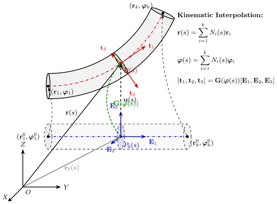
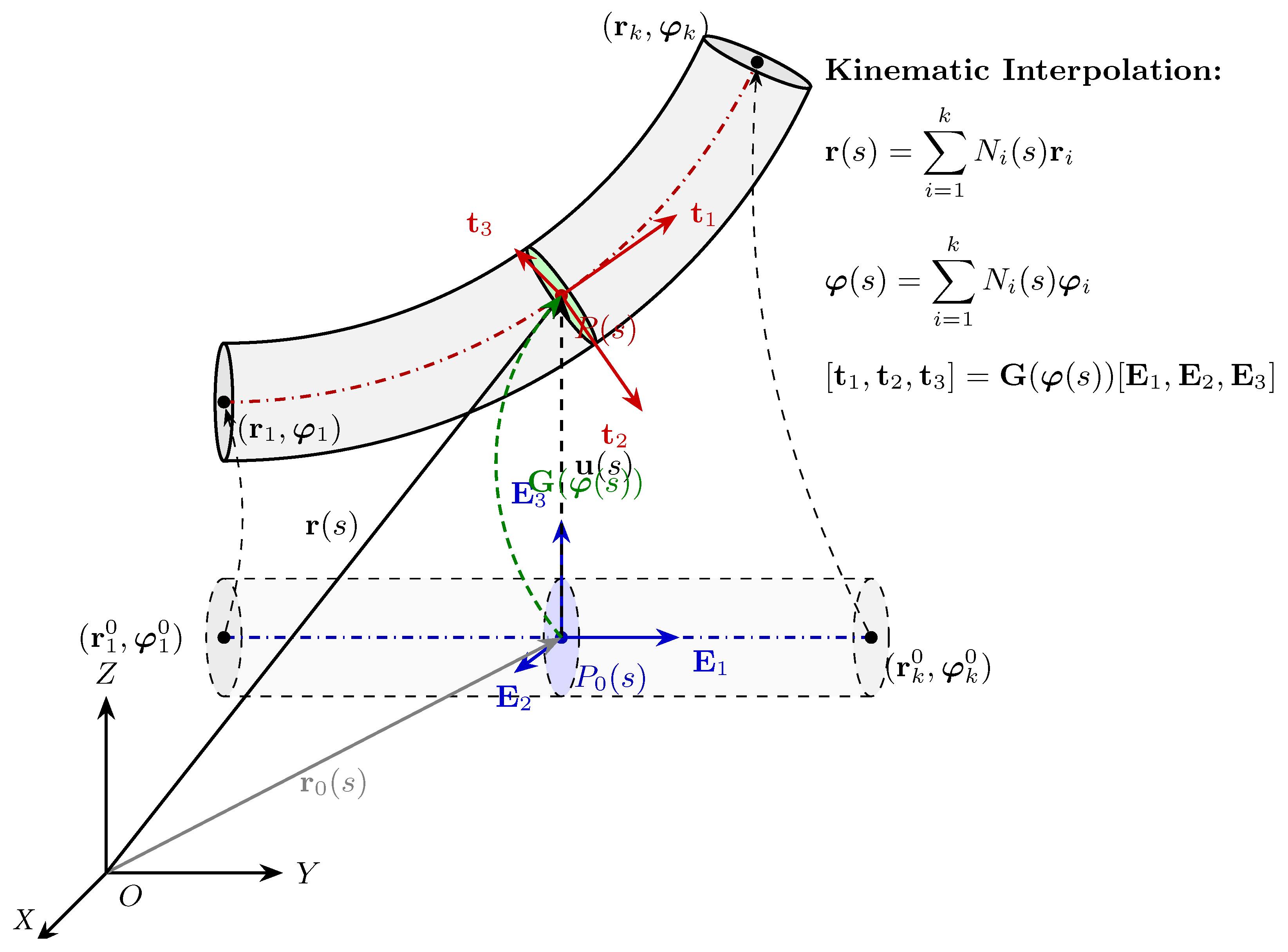
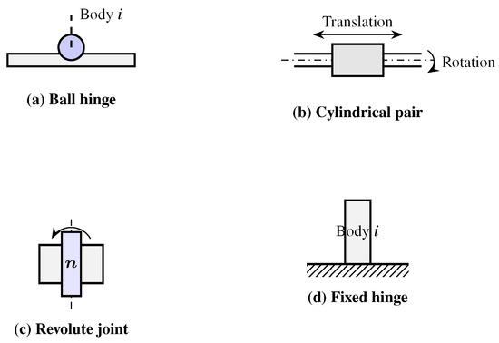
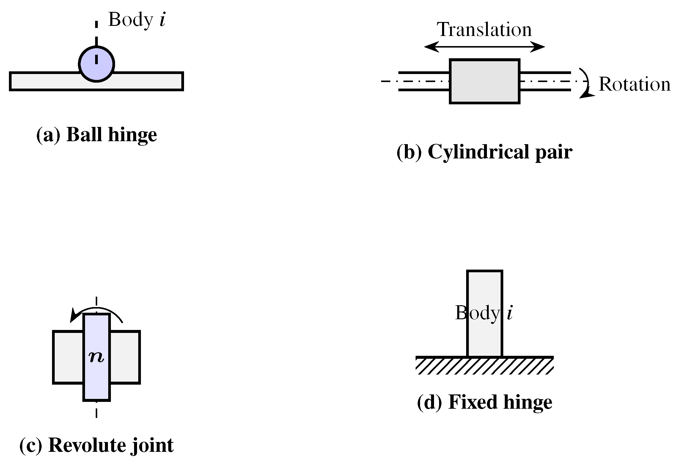
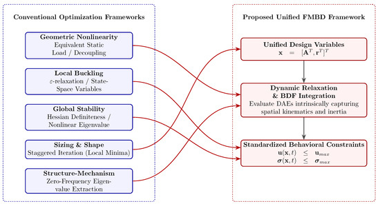
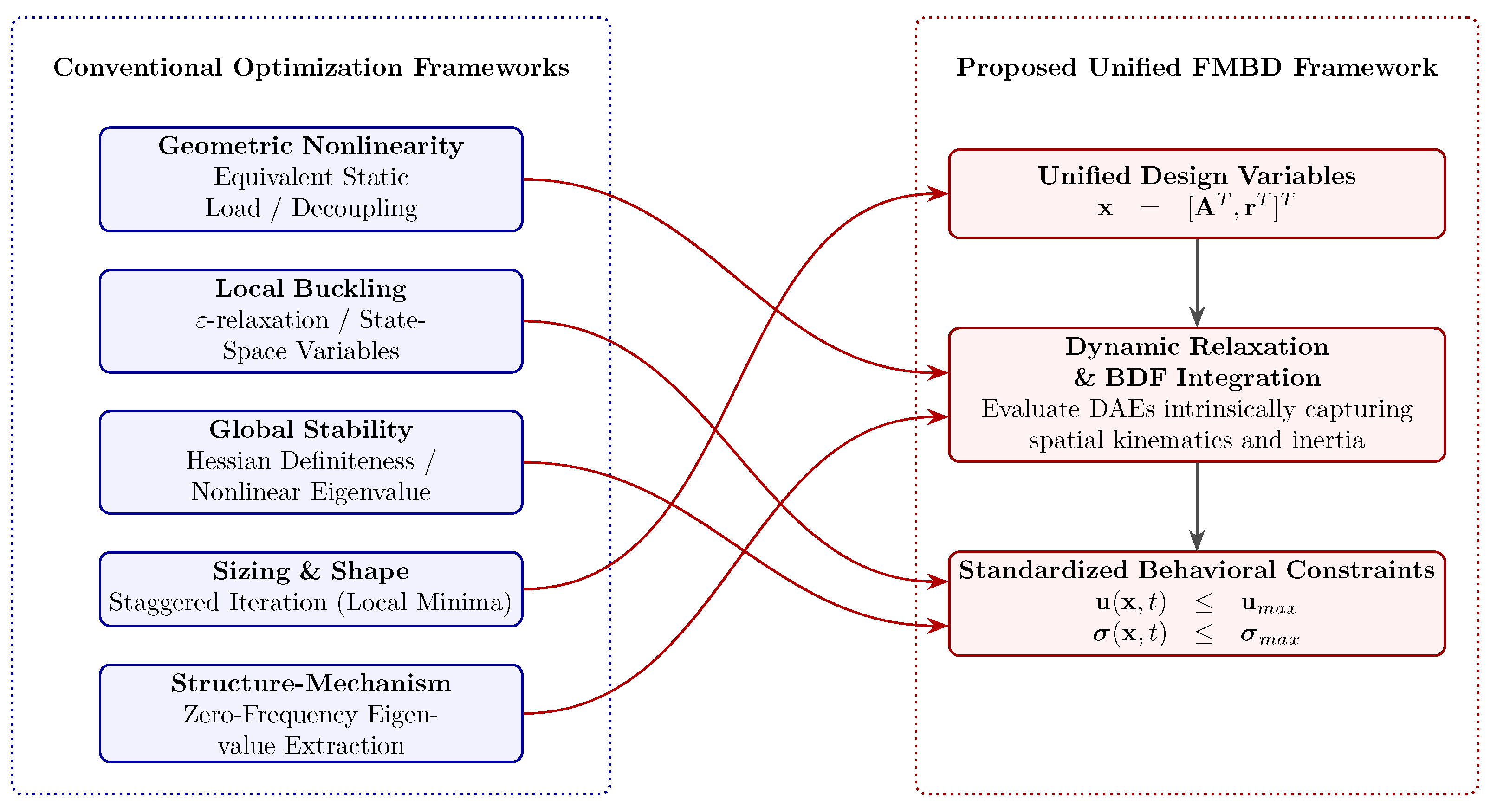
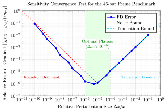
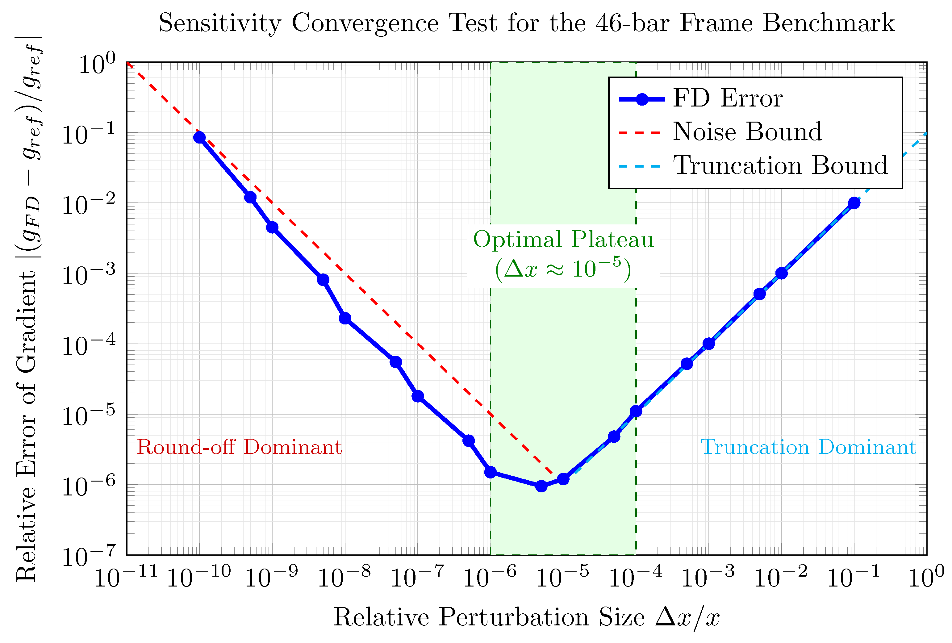
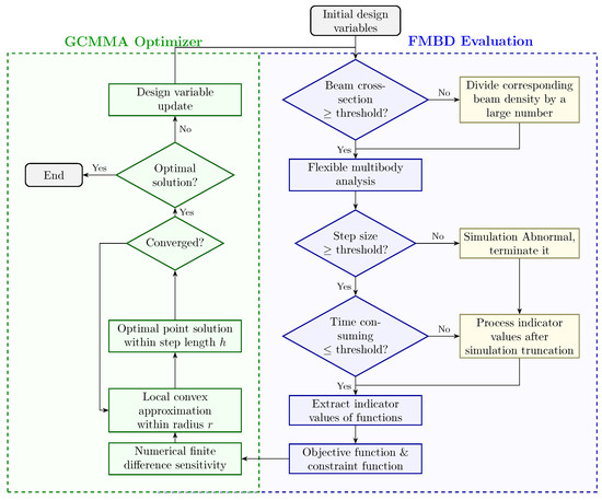
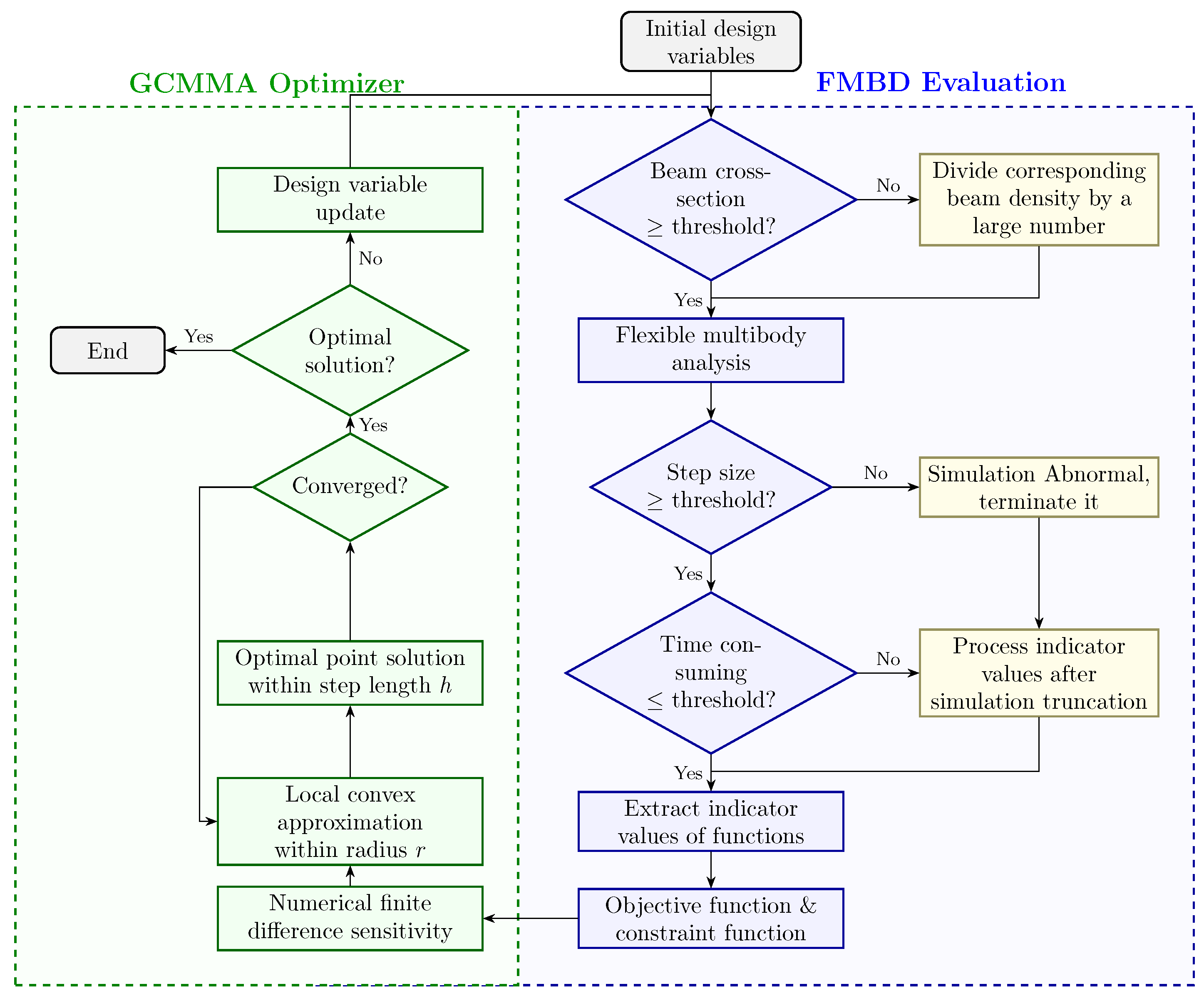
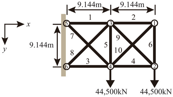
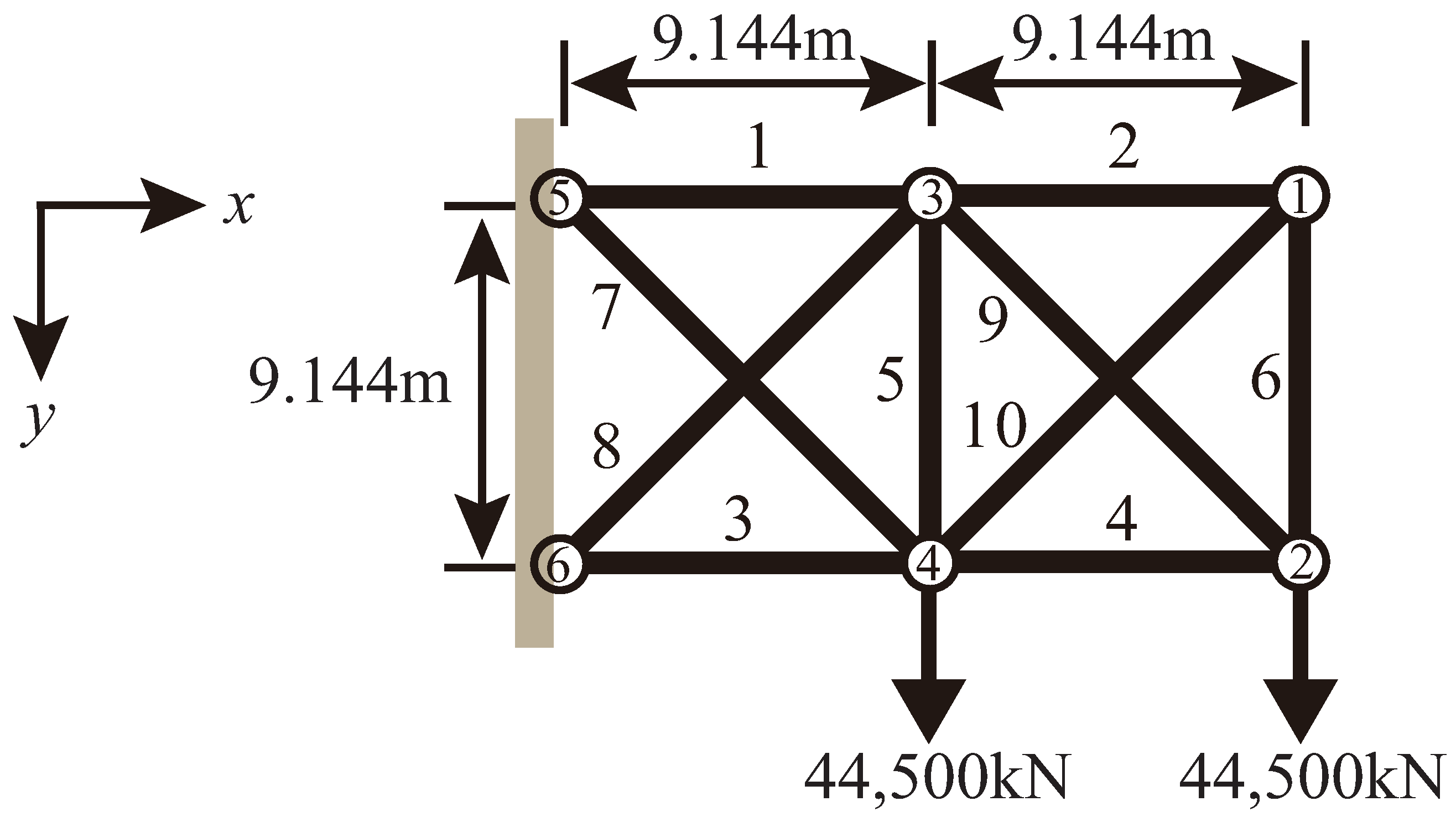
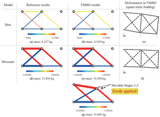
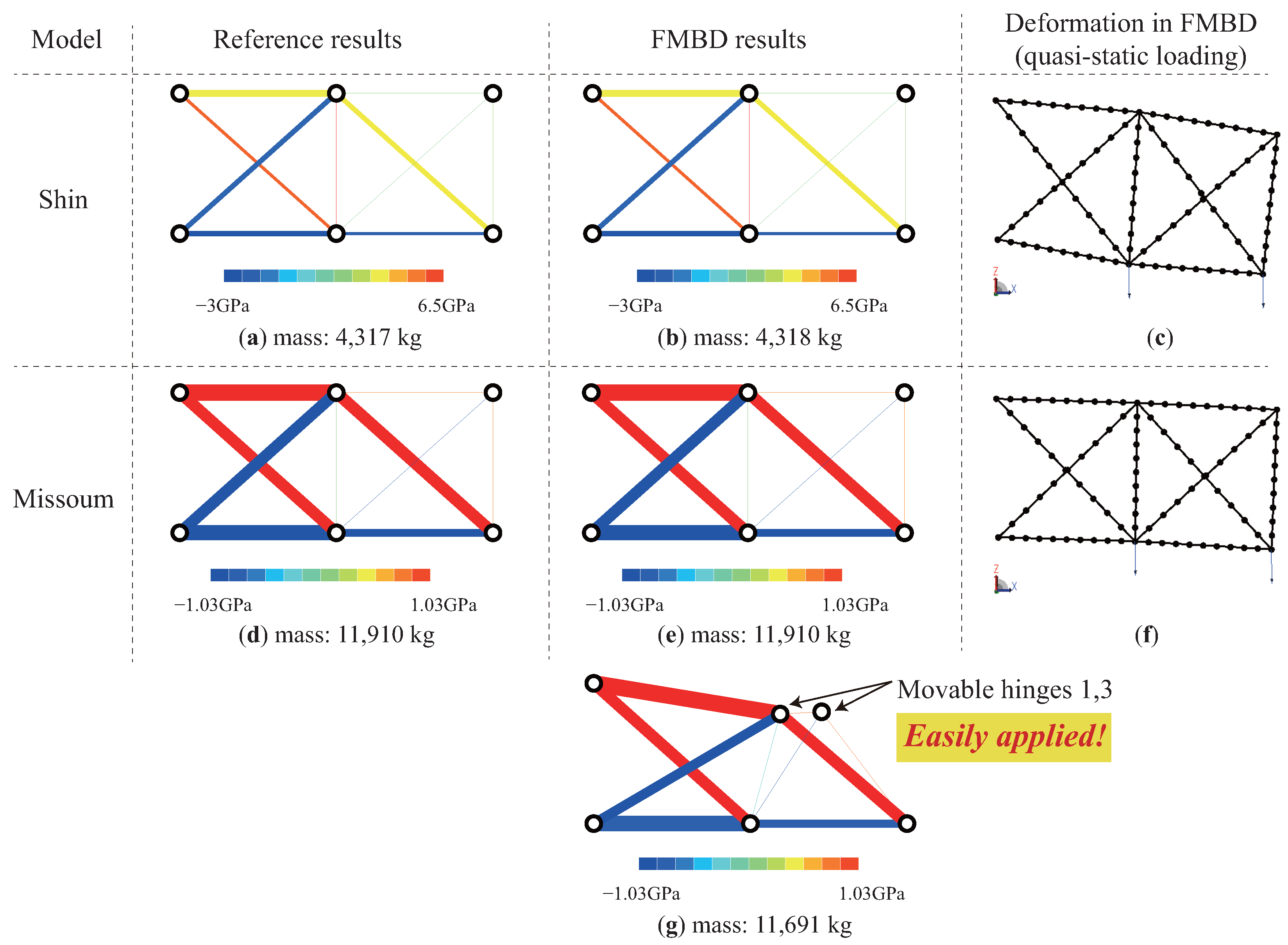
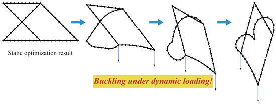
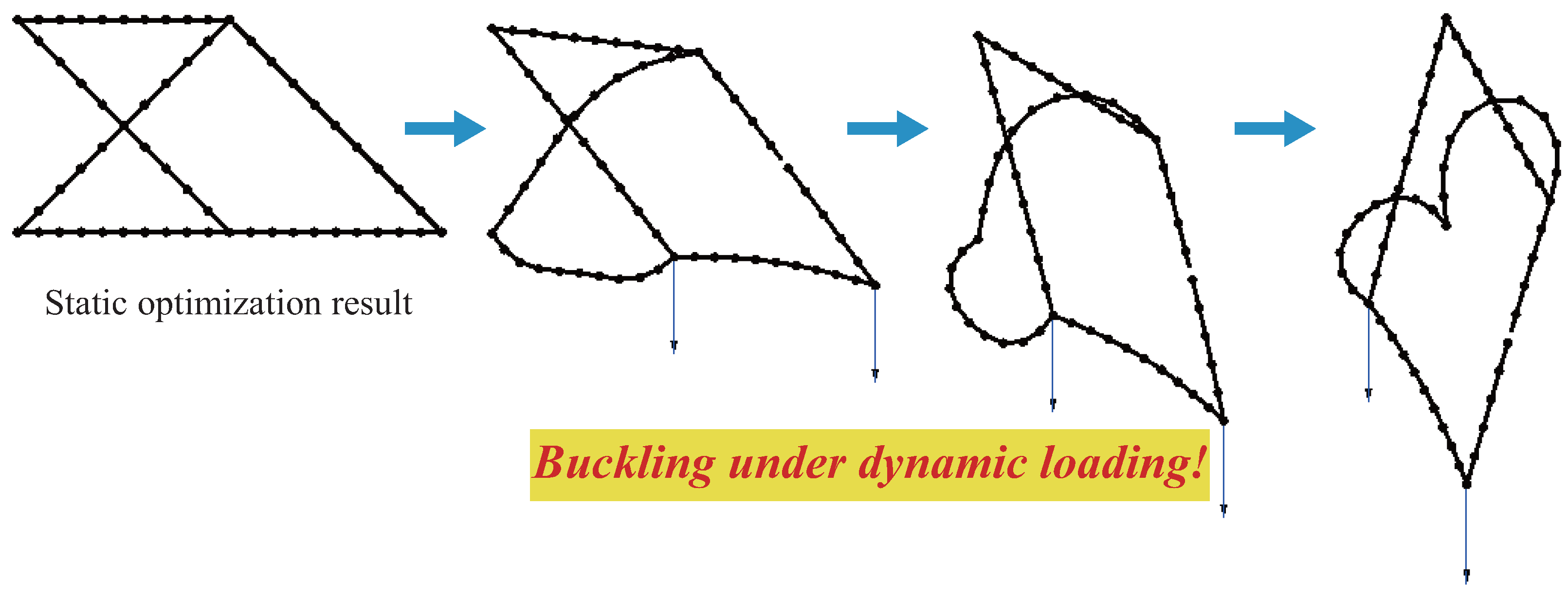
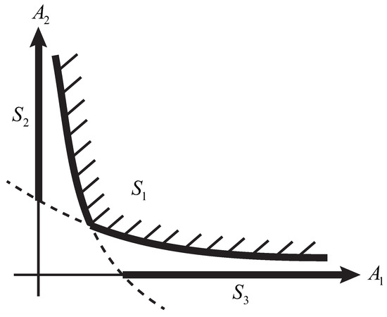
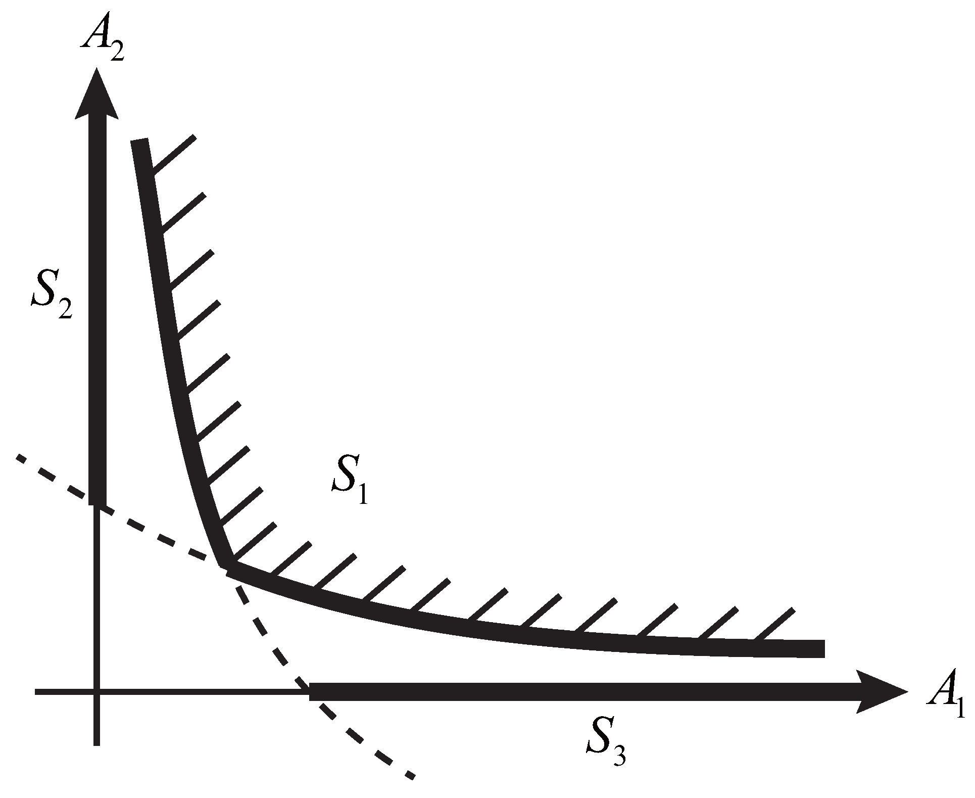
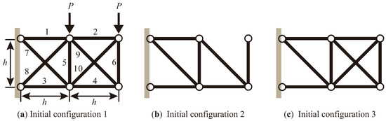
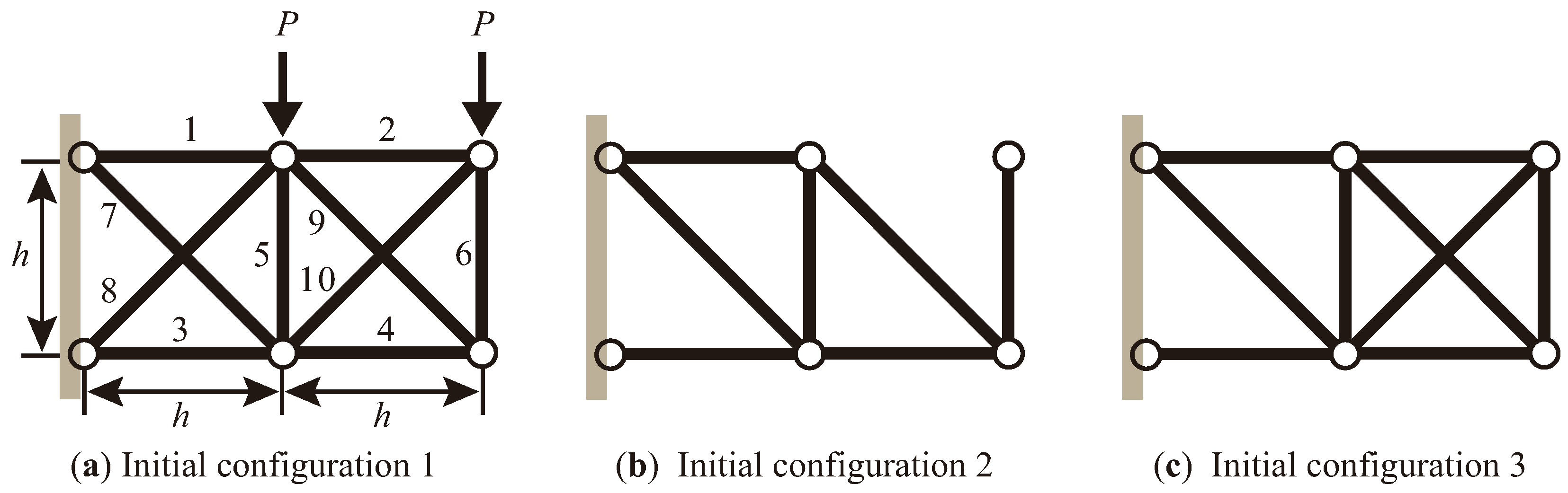
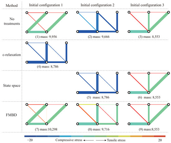
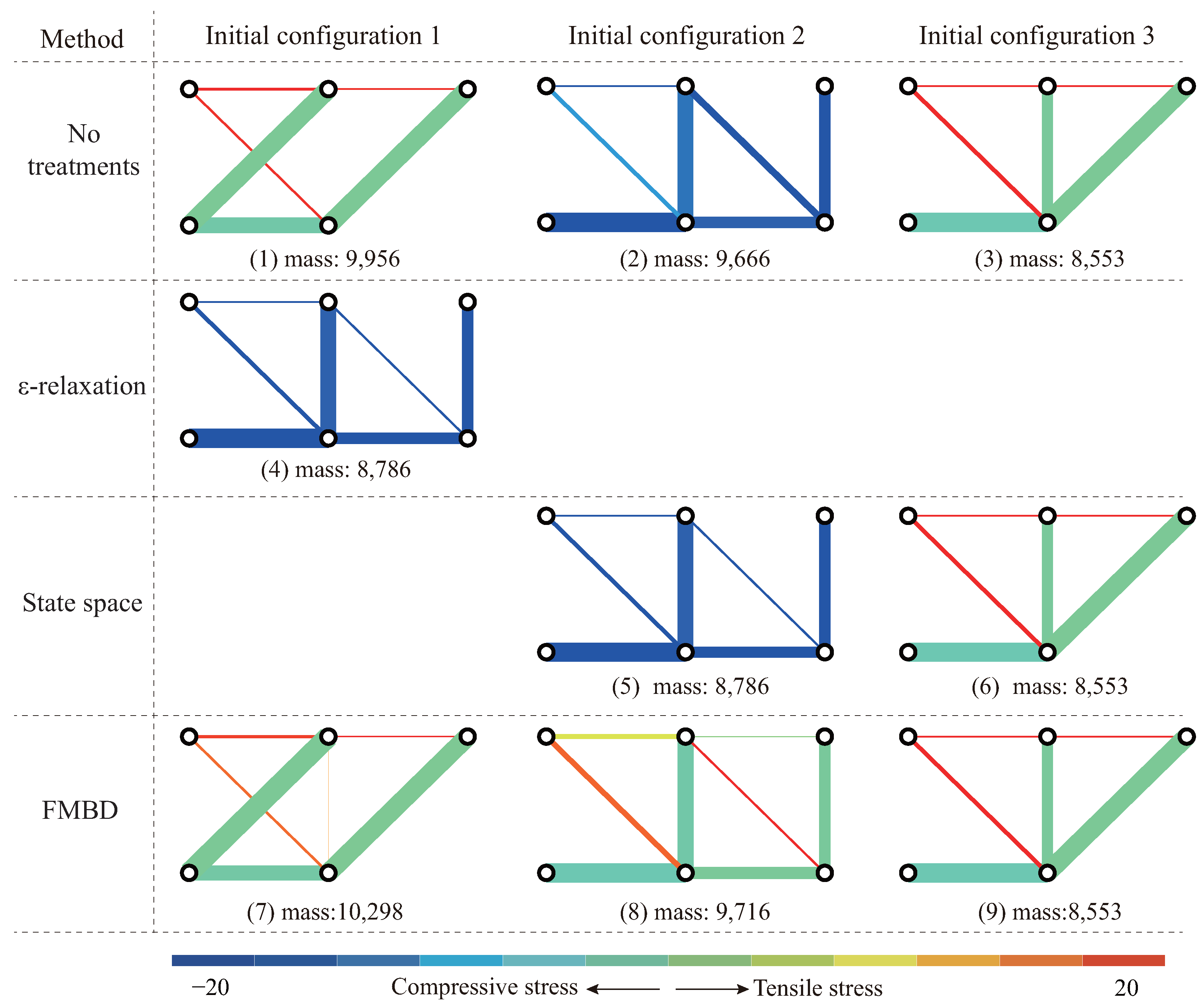
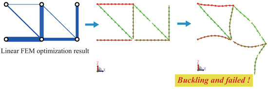
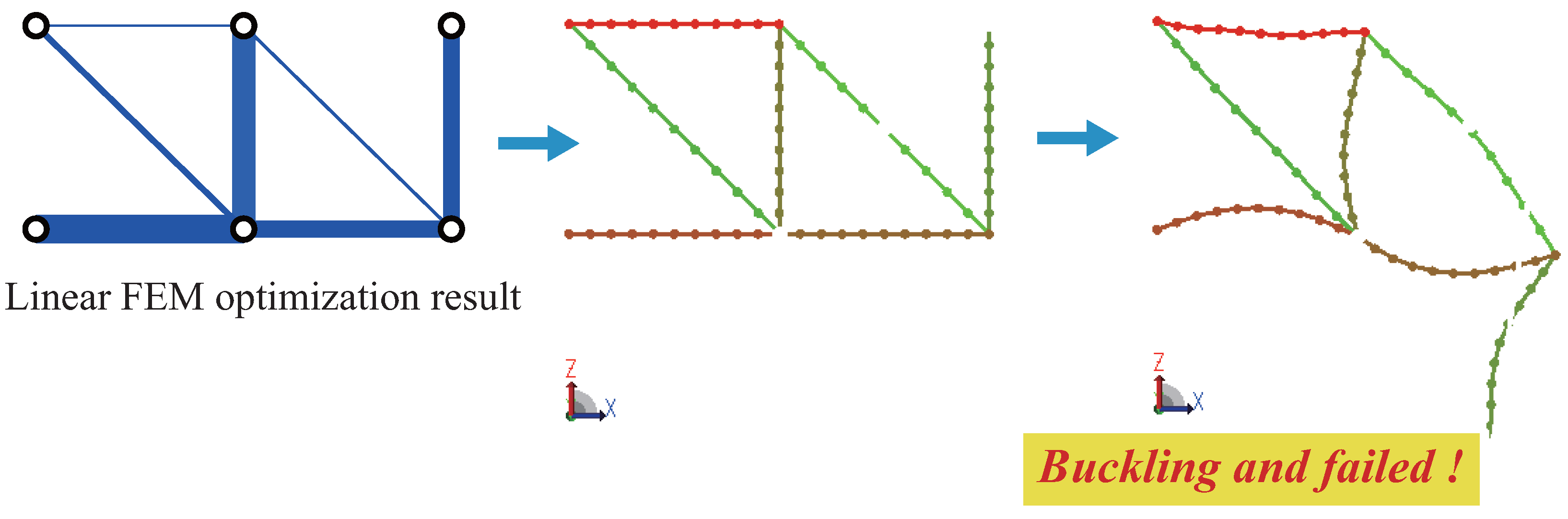
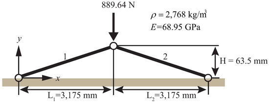
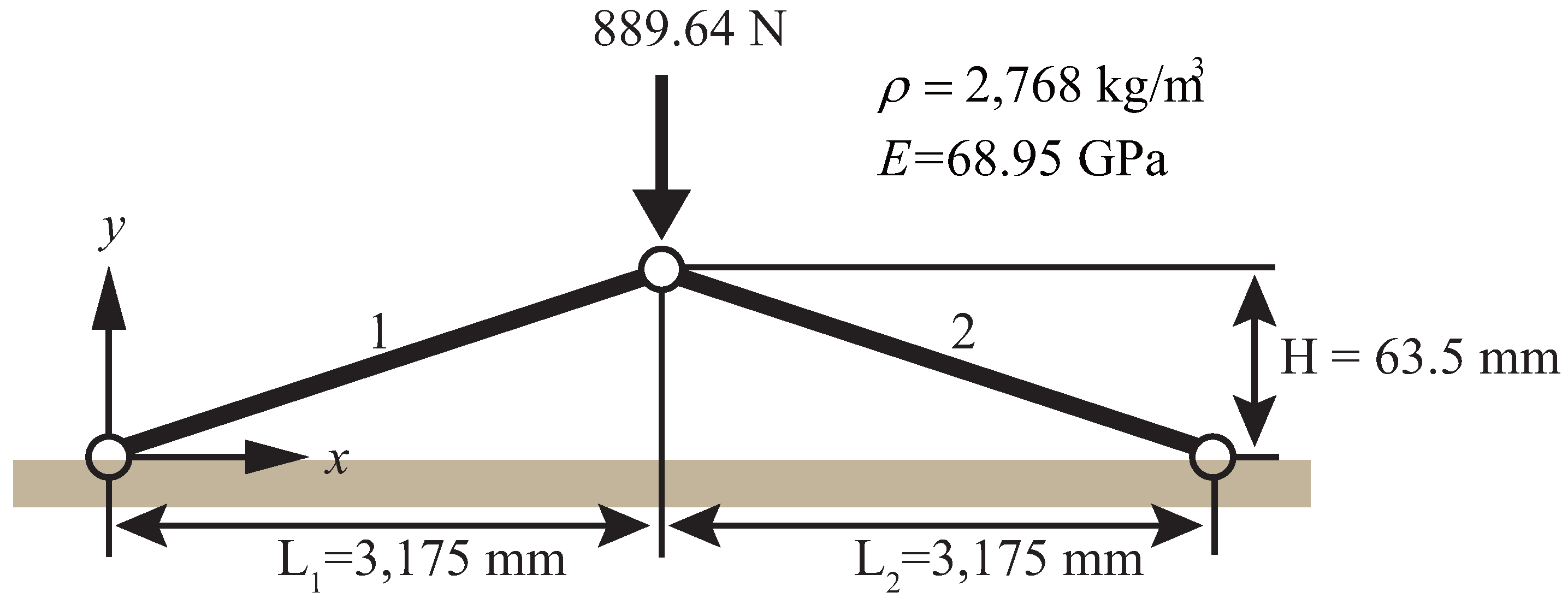
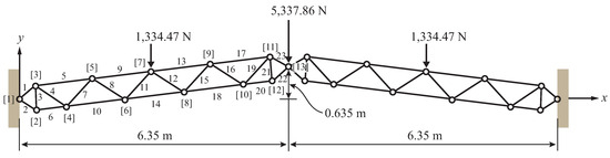
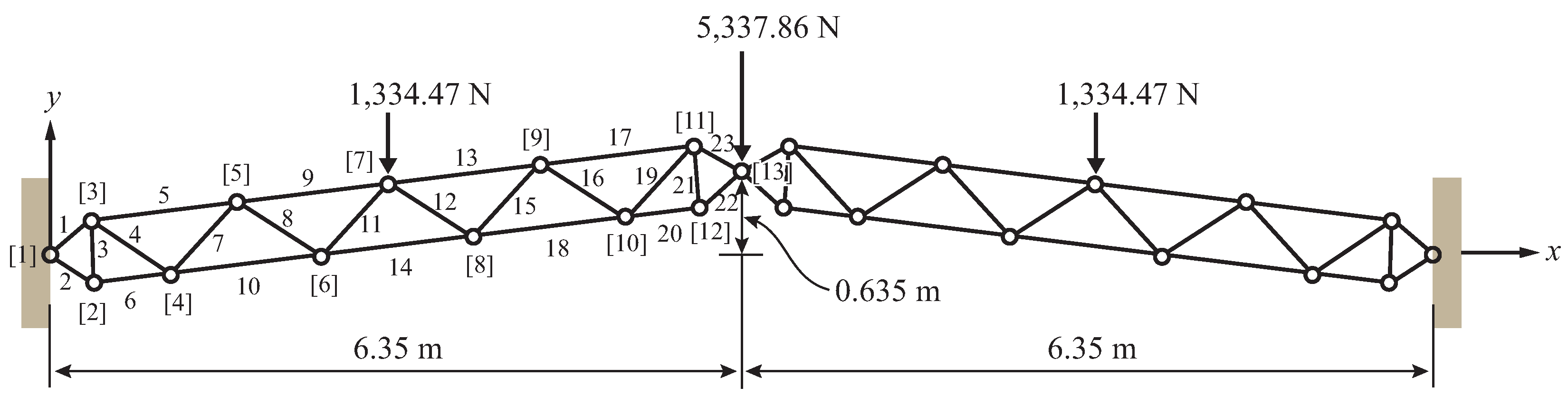
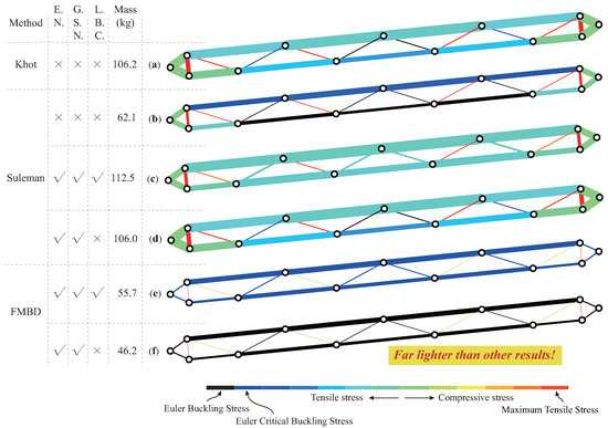
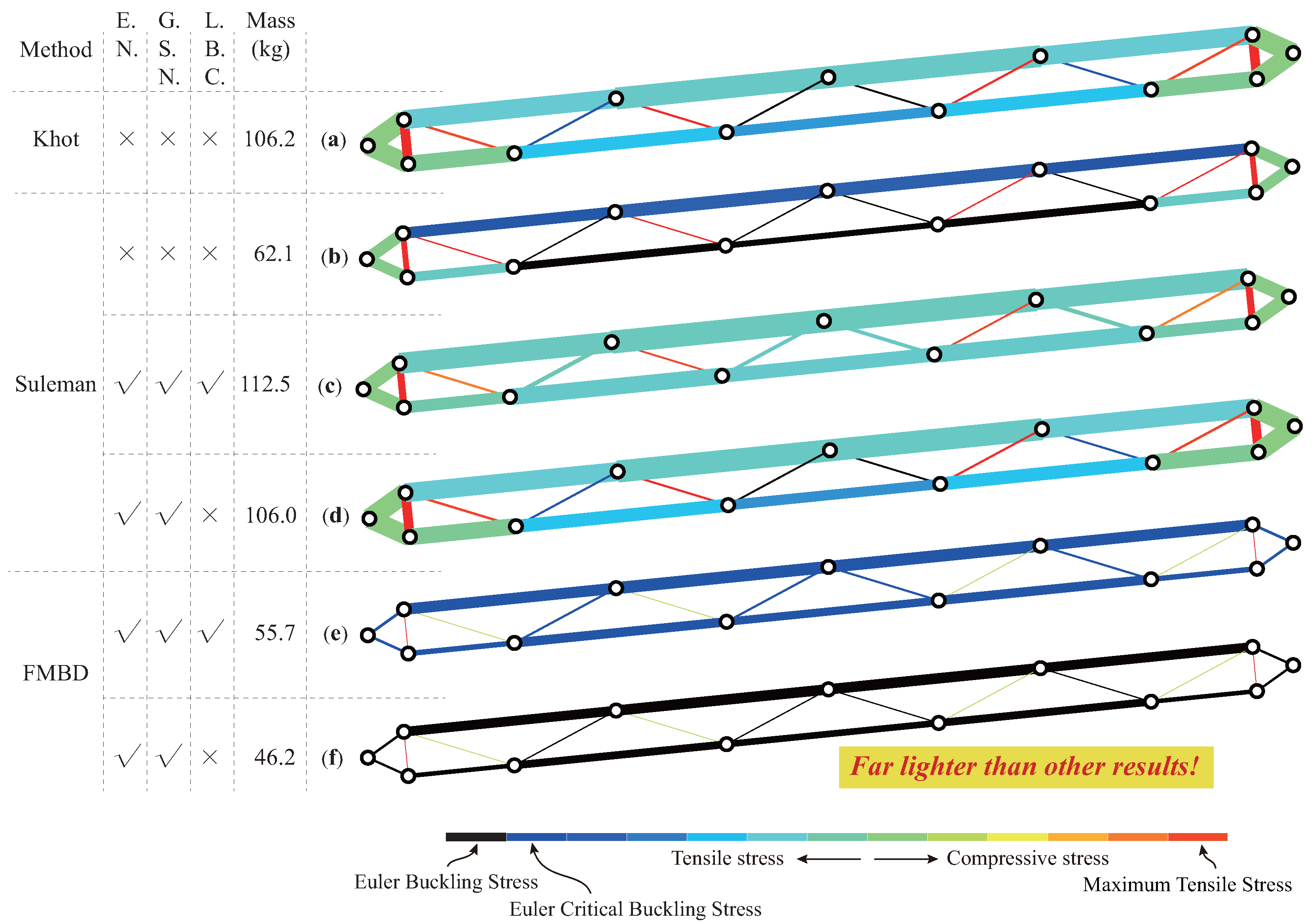


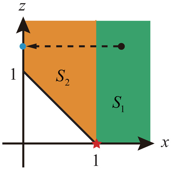
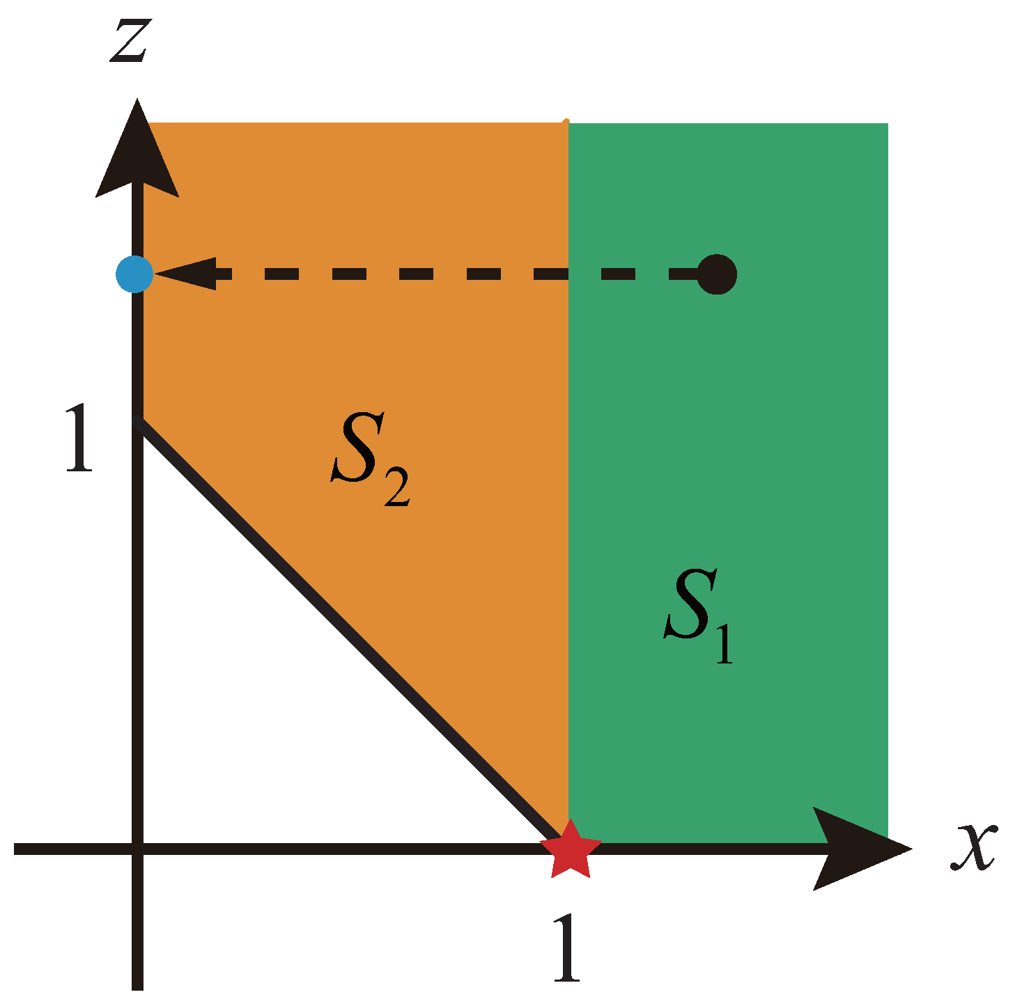
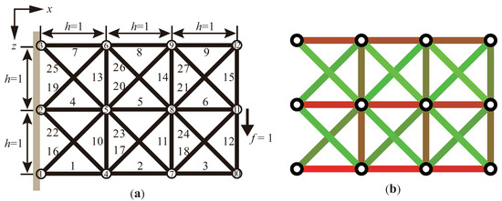
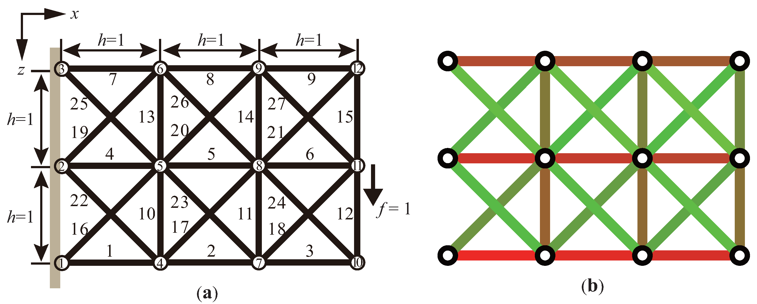
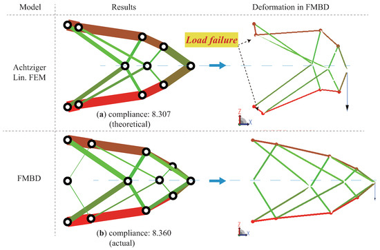
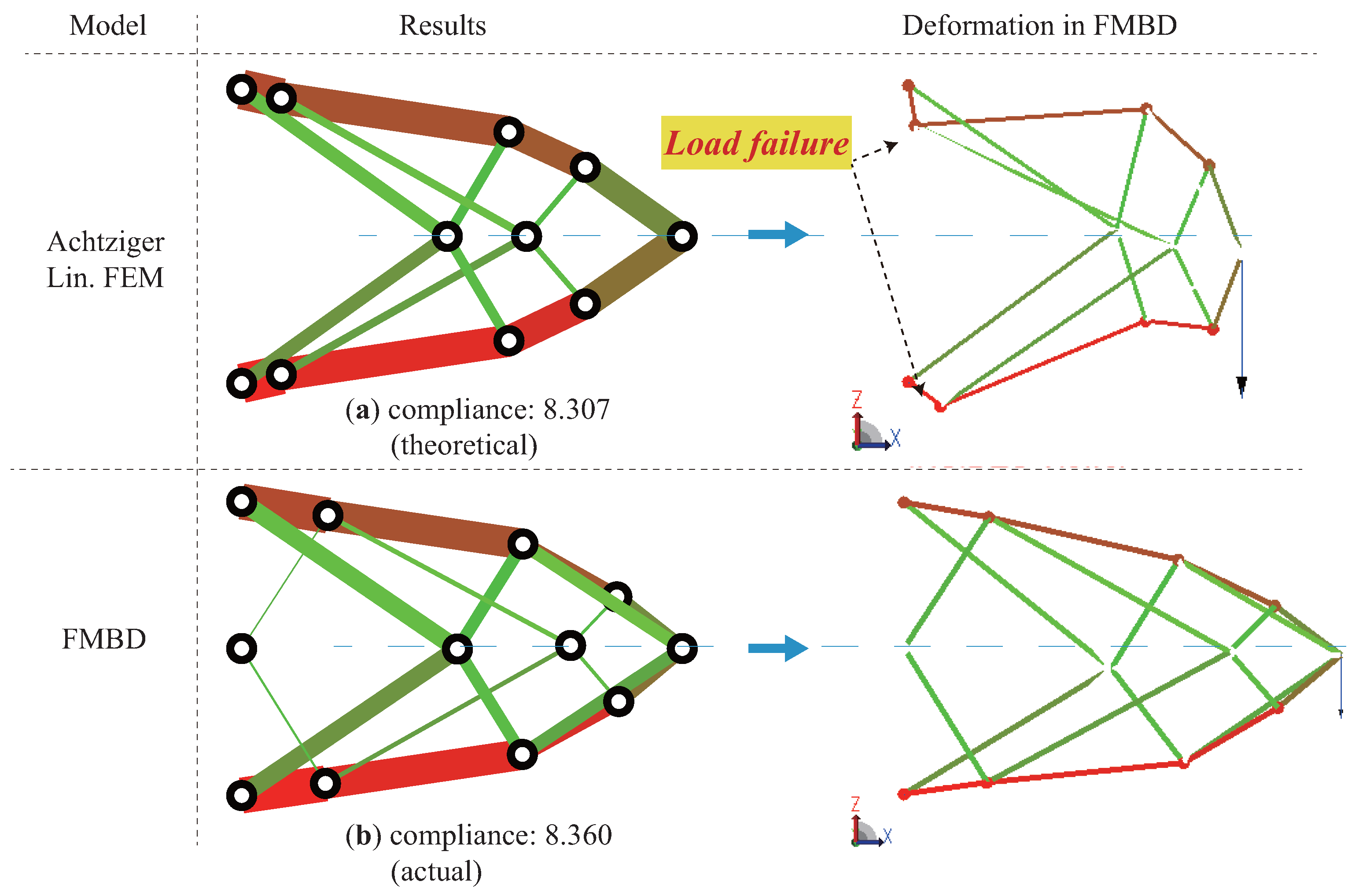
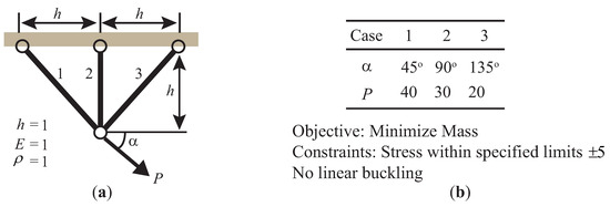
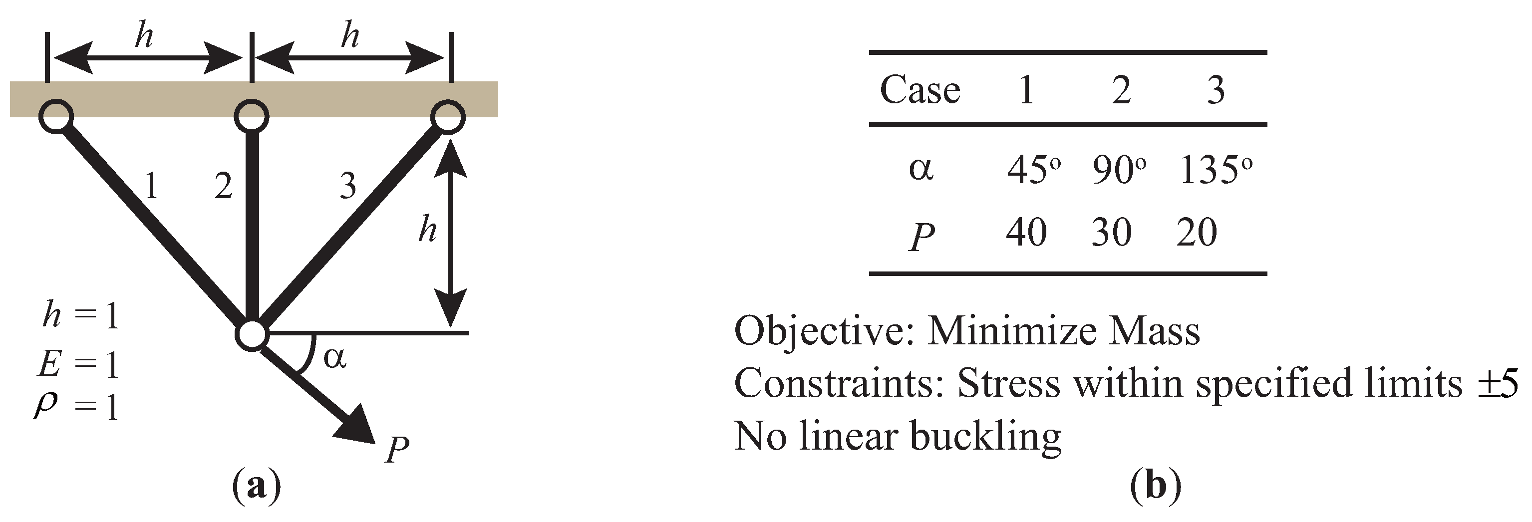
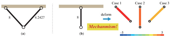
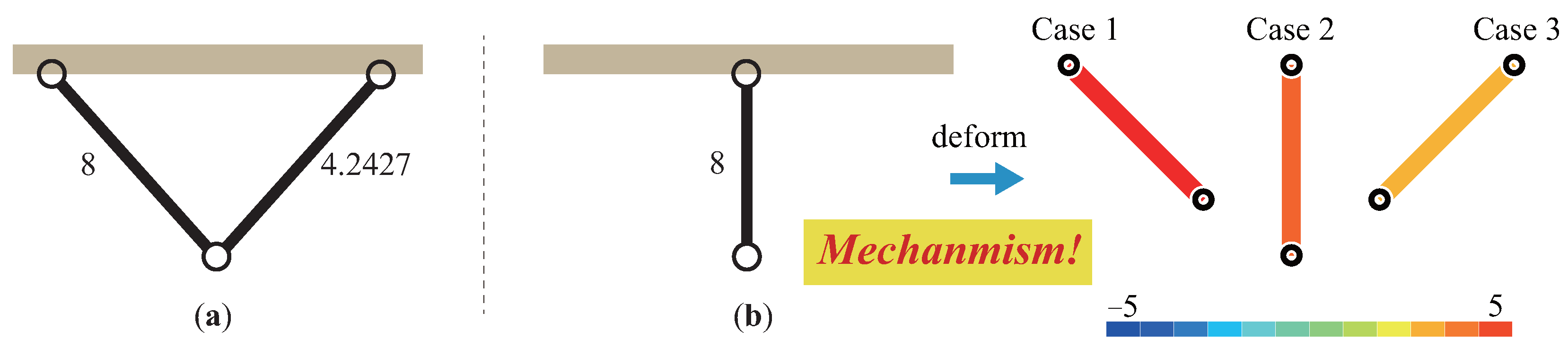
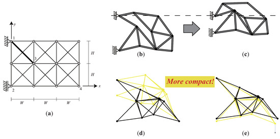
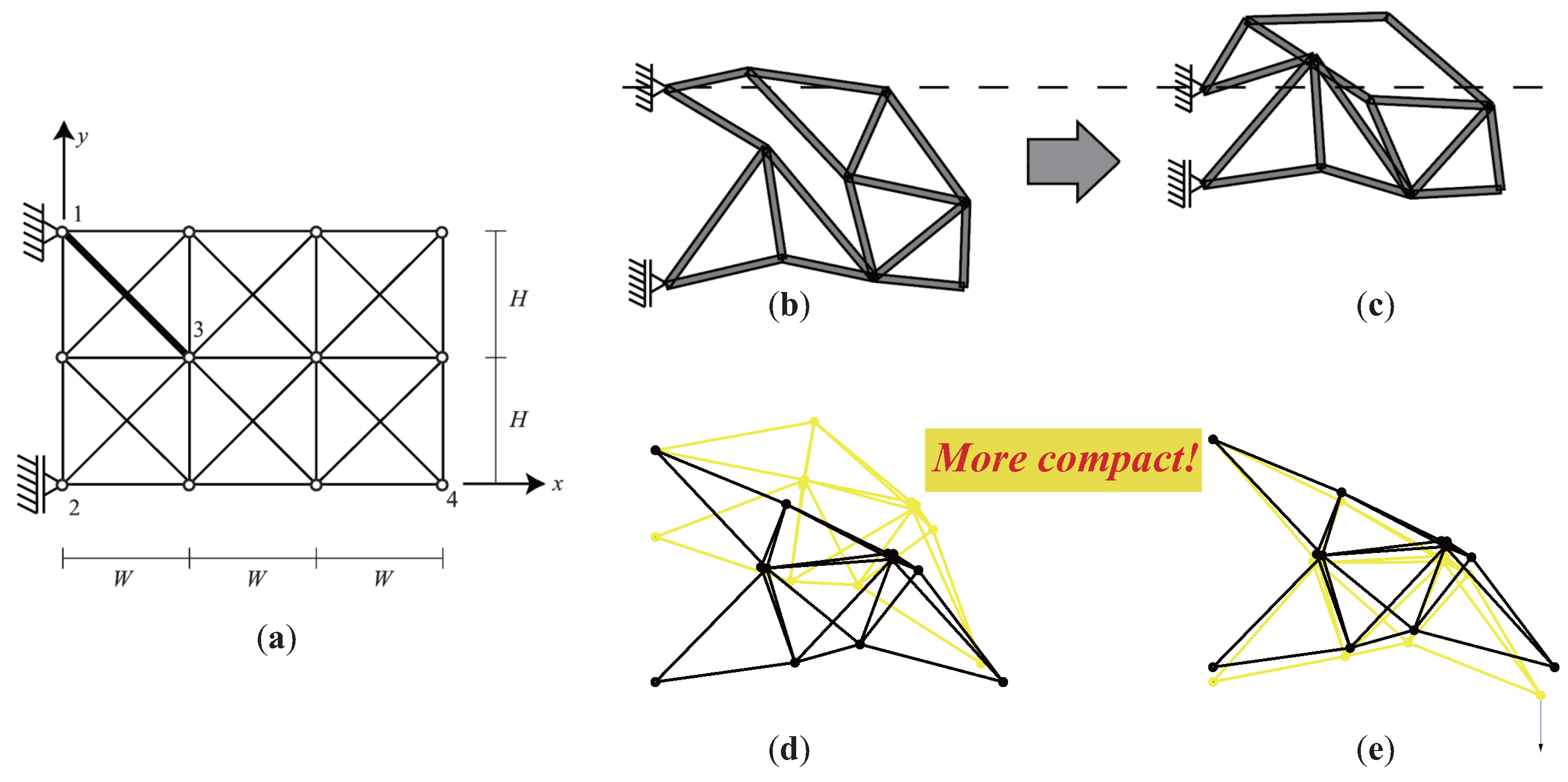

Disclaimer/Publisher’s Note: The statements, opinions and data contained in all publications are solely those of the individual author(s) and contributor(s) and not of MDPI and/or the editor(s). MDPI and/or the editor(s) disclaim responsibility for any injury to people or property resulting from any ideas, methods, instructions or products referred to in the content. |
© 2026 by the authors. Licensee MDPI, Basel, Switzerland. This article is an open access article distributed under the terms and conditions of the Creative Commons Attribution (CC BY) license.