Morphological and Environmental Drivers of Urban Heat Islands: A Geospatial Model of Nighttime Land Surface Temperature in Iberian Cities

Abstract

This study explores how urban morphological and environmental factors influence Urban Heat Islands (UHIs) using a geospatial modeling approach. The aim of the research is to develop a methodology to assess UHI effects, emphasizing the role of urban morphology, land use, and vegetation in nighttime heat accumulation. A micro-scale analysis with a 50 m resolution is conducted by integrating a custom QGIS plugin with open-access data, ensuring broad applicability. The 50 m resolution was chosen because it allows for the capture of local variations in UHI intensity while maintaining the scalability of the urban analysis across different city contexts. Non-parametric statistical analyses (ANOVA, Kruskal–Wallis H test, and correlation assessments) were used to evaluate the relationships between the urban parameters—wind corridors, altitude, vegetation (NDVI), surface water (NDWI), and the Sky View Factor (SVF)—and Nighttime Land Surface Temperature (LST). Given that UHI variations during summer, particularly in cities of the Iberian Peninsula, are closely linked to summer heat severity, this factor was considered to classify the cities for the study. Correlation analyses confirm that all tested factors influence LST, with wind corridors being the least significant. The model performance evaluation shows the highest errors in cities with lower summer severity (RMSE = 1.586 °C, MAE = 1.2686 °C, MAPE = 6.99%) and the best performance in warmer cities (RMSE = 1.4 °C, MAE = 1.14 °C, MAPE = 4.5%). Validation in four cities of the Iberian Peninsula confirmed the model’s reliability, with the worst RMSE value of 2.04 °C. These findings contribute to a better understanding of the factors driving UHIs and provide a scalable assessment framework.

1. Introduction

Urbanization is reshaping city size and morphology worldwide. The global urban population is expected to rise from 56% to 68% by 2050 [1]. This expansion replaces natural landscapes with built environments, altering regional climates and generating distinct urban microclimates. One of the most studied effects is the Urban Heat Island (UHI), characterized by elevated temperatures in urban centers compared to surrounding rural areas. First documented by Howard [2], UHIs arise from high heat retention in dense urban structures, reduced vegetation, and anthropogenic activities [3]. Recent satellite studies confirm its intensification in metropolitan areas, such as Houston, Texas [4], underscoring the value of remote sensing for tracking UHI dynamics and evaluating mitigation strategies.

UHI development results from a complex interaction of urban morphology, land cover, vegetation, and building materials, all influencing heat absorption and retention. Increased building height and density exacerbate heat accumulation, particularly in megacities with restricted airflow [5]. UHI intensities vary widely, from 2 °C in small cities to over 12 °C in dense metropolitan areas [6]. However, although UHI intensities exceeding 12 °C have been reported under specific conditions, typical values range from 2 °C to 4 °C depending on urban morphology and climatic context. Differences in magnitude stem from methodological approaches, climatic conditions, and urban configurations, highlighting the need for standardized measurement frameworks [7]. Moreover, urban design plays a key role in air circulation and thermal radiation, with compact, multi-story structures amplifying the UHI effect [8].

Beyond temperature increases, UHIs influence energy consumption, thermal comfort, and public health. Higher urban temperatures drive up cooling demands, increasing energy use and peak electricity loads [9,10]. Additionally, temperature rises correlate with higher mortality rates, with up to a 2.72% increase in mortality per additional degree above optimal thresholds [11,12]. Meteorological factors such as wind speed and atmospheric stability modulate UHI intensity by affecting heat dispersion [13,14]. Studies in cities like Seoul and Łódź demonstrate how wind dynamics and land use shape UHI distribution [15,16]. In the context of global warming and rapid urbanization, UHIs pose a major challenge for sustainable urban development and livability [17,18].

Despite extensive research, the main drivers of UHIs and the most effective mitigation strategies remain subjects of debate. Some studies emphasize urban morphology [8], while others focus on wind dynamics and heat transport [7]. Modeling urban wind behavior remains complex due to data limitations, whereas urban morphological factors—such as building height, density, and spatial configuration—are more readily quantifiable using satellite imagery and geospatial databases. Research confirms that urban morphology significantly influences microclimates, with elements like street canyon morphology, vegetation cover, and land surface permeability affecting UHI intensity [19,20,21]. In several cities across France, specific morphological characteristics, such as height-to-width ratios and sky view factors, have been linked to UHI variation [22].

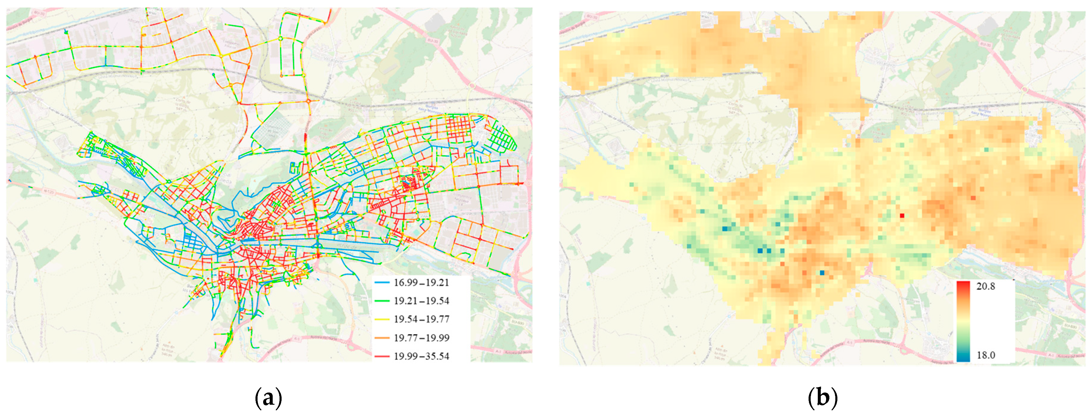
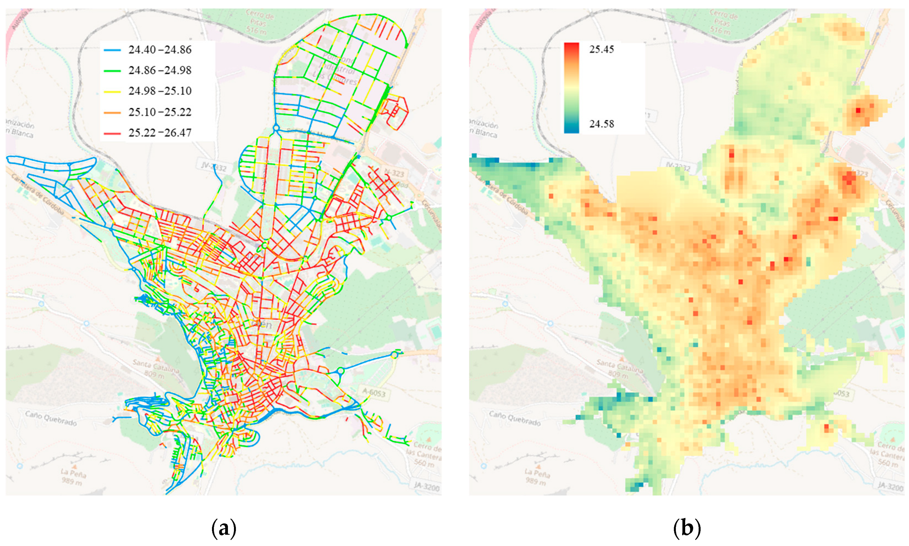
This study calculates Land Surface Temperature (LST) at the road segment level, using 50 m road sections as analytical units to integrate morphological and environmental assessments. LST is considered as a sign of a UHI, being a parameter that measures its expression, Surface Urban Heat Island (SUHI) [23]. Roads are considered in this work as a measurement unit due to their extensive urban presence and their role in thermal dynamics. Specifically, roads can be used as containers of the surrounding morphological and environmental conditions. This structured approach enables a standardized evaluation of localized heat accumulation and its contribution to UHIs, positioning streets as key spaces for large-scale mitigation measures.

Urban climate research increasingly utilizes the Local Climate Zone (LCZ) classification to understand spatial patterns of UHI intensity [24]. Recent studies, such as [25], have demonstrated the value of LCZs in relating Land Surface Temperature (LST) and air temperature distributions at fine spatial scales. Although this study does not explicitly apply an LCZ framework, it indirectly incorporates key morphological and environmental descriptors analogous to LCZ parameters, ensuring comparability while maintaining flexibility based on openly available raw datasets.

Existing UHI assessment methods often face limitations related to data accessibility (especially atmospheric and meteorological, as well as morphological) and computational demands [7,26]. While physical models require detailed morphological, atmospheric, and meteorological data, remote sensing methods may lack the resolution to capture localized thermal variations [27,28]. To bridge these gaps, this study adopts a morphology-based approach, analyzing how building height, density, design, and green space distribution influence heat retention. Additionally, it incorporates moisture levels via surface water bodies and solar radiation through the Summer Climate Severity (SCS) index.

The inclusion of a climate severity metric is grounded in prior efforts to quantify summer thermal stress and its effects on urban systems. One of the earliest anthropocentric indices [29] was originally developed for the northeastern United States, though its global applicability remains unverified. In Europe, a Climatic Severity Index was proposed [30] to define summer climatic zones in Italy, linking them directly to air conditioning energy demand in buildings. In a similar manner, the Spanish Building Code (CTE) introduced a classification of summer climatic zones in the Iberian Peninsula based on accumulated summer degree-days. This national-level approach provides a standardized, regulation-backed index for quantifying summer climatic severity, which serves as the foundation for the SCS used in this study.

This methodological framework aligns with recent research advocating for morphology-based UHI assessments, particularly in Mediterranean contexts where compact urban structures significantly modulate temperature distributions [31,32].

To enhance practical applicability, this work develops a custom QGIS plugin for streamlined data processing and broad usability across different urban contexts. Statistical techniques, including ANOVA and correlation analyses, reinforce the reliability of the findings. This comprehensive framework not only advances LST-based UHI research but also provides actionable insights for urban planning, supporting evidence-based strategies for mitigating UHIs in diverse climatic zones.

The Iberian Peninsula was selected as the study area due to its varied climatic and urban characteristics. The findings will serve as a foundation for replicating this approach in other cities with similar geographical contexts, advancing UHI research and supporting data-driven urban policies.

The remainder of this paper is structured as follows: Section 2 details the data sources, parameters, and methodology for UHI modeling. Section 3 presents statistical results and discussion. Section 4 presents model applicability across urban environments, and Section 5 summarizes key insights.

2. Materials and Methods

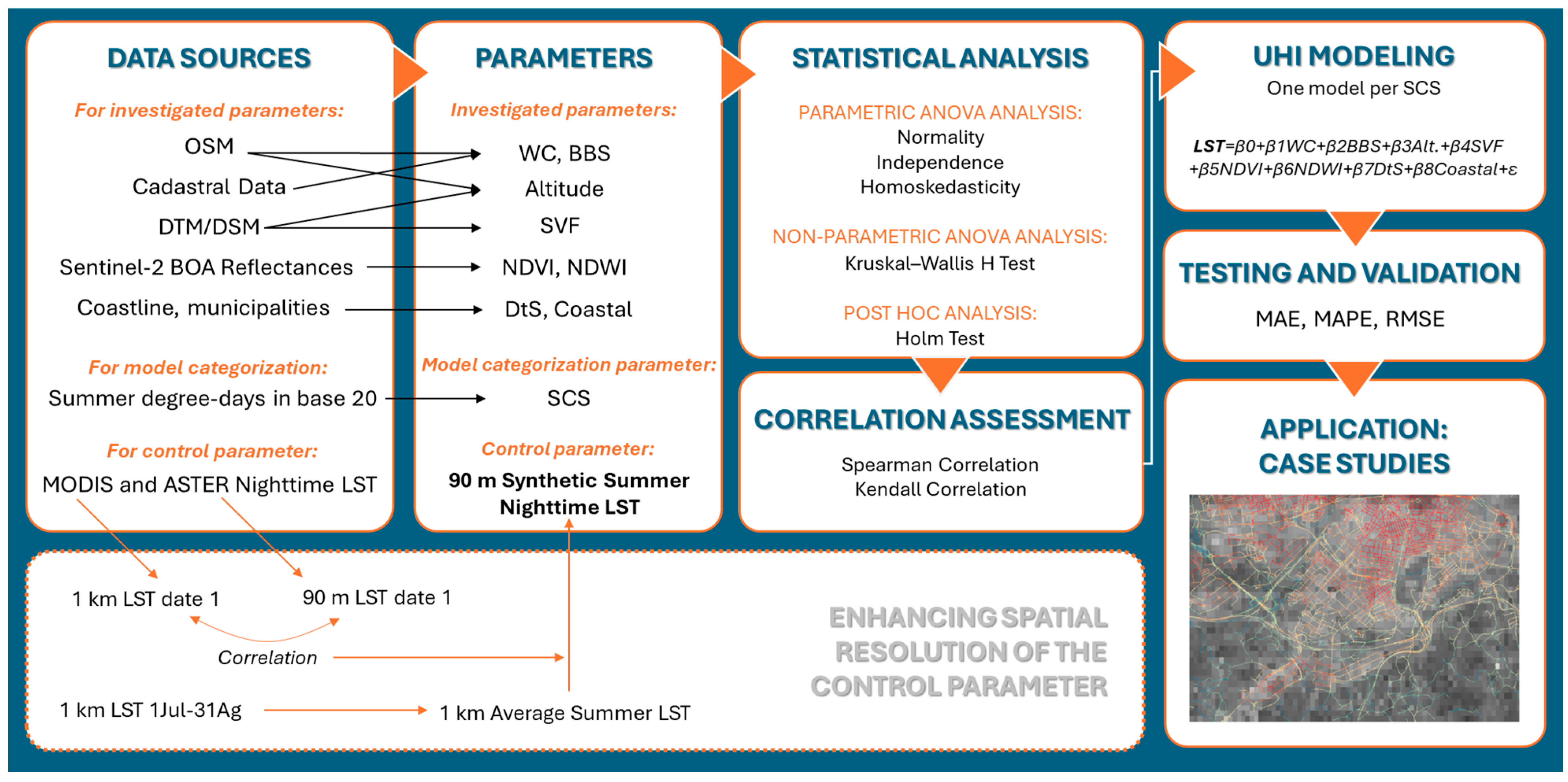
The proposed methodology for characterizing UHIs (Figure 1) involves morphological and environmental parameters to understand their influence on the gradual accumulation of heat in city centers. This approach characterizes UHIs at a 50 m street or road scale, as illustrated in Figure 1. Key factors considered include street and building geometry, SVF, altitude, vegetation, and water bodies (using spectral indices), and SCS. The study covers the summers of 2021, 2022, and 2023, considering July and August for each year as the peak heat period.

To ensure precision and efficiency, we developed a custom plugin for Quantum GIS (QGIS ©, available at: www.qgis.org (accessed on 10 January 2025)), which automates all necessary operations using predefined information layers. The plugin enhances reproducibility and minimizes human error, ensuring that parameter calculations adhere to rigorous scientific standards.

This methodology assesses the relationship between each selected parameter and nighttime surface temperature, specifically to the 90 m synthetic average summer LST at night. Below, we detail the data sources for parameter computation, followed by the statistical and correlation analyses conducted using the R programming language (v.4.3.0).

2.1. Data Sources

To ensure global applicability and replicability, all data sources follow the Open Data principle and provide global coverage. Based on the two main evaluation criteria—urban morphology and urban environmental conditions—the data sources are categorized as follows:

2.1.1. Urban Morphology Data Sources

Urban morphology describes the physical structure of human settlements, and several parameters, such as wind corridors, altitude, green spaces, and hydromorphology, are considered. The data sources include:

• OpenStreetMap (OSM): Provides street-level data on roads, buildings, and urban infrastructure, accessed via the QuickOSM plugin (Section 3).
• Cadastral Data: Offers detailed land use and property boundary information. Data for this study was sourced from the General Directorate of the Spanish Cadastre.
• Digital Terrain and Surface Models (DTM/DSM): all data was sourced from the Spanish Geographic Institute (IGN), aligned with the INSPIRE Directive. The following specific data were used:
  • DTM at 2 m resolution, providing elevation data, crucial for computing street altitudes.
  • DSM at 2 m resolution, used to calculate the SVF.
  • Building height model at 2.5 m resolution that helps estimate wind corridors, influencing UHI formation.
• Coastline and Municipality Boundaries: used to determine the distance of a city to the sea and to classify cities as coastal or non-coastal. These data were sourced from the IGN.

2.1.2. Urban Environmental Data Sources

Urban environmental conditions influence urban heat islands (UHIs) through vegetation cover, water presence, SCS, and LST. The data sources used in this study include:

• Sentinel-2 BOA Reflectances: Captured by the Multispectral Imager (MSI) sensor aboard Sentinel-2 satellites of the European Satellite Agency (ESA), which have 10 m spatial resolution. These atmospherically corrected measurements are used to derive spectral indices (e.g., the NDVI and NDWI) for monitoring vegetation and water bodies in the city.
• Summer degree-days in base 20: This historical summer temperature data servers to classify cities based on the severity of their summers, the SCS index was used, following the Spanish Building Code (CTE). The index relies on degree-days (DD) at a base temperature of 20 °C, using data from AEMET (Spanish Meteorological Agency).
• MODIS and ASTER Nighttime LST: To use summer nocturnal LST as reference parameter in the model, we created a synthetic night LST image with a 90 m spatial resolution based on the average summer nighttime LST. This approach addresses the absence of an open product from ESA or NASA that offers both adequate spatial and temporal resolution for this purpose. Thus, we integrated the spatial detail of ASTER with the temporal frequency of MODIS, following methods previously validated in UHI studies (e.g., ref. [33]). Quality control was applied to remove extreme temperature anomalies or cloud interference.
  • MODIS with 1 km resolution, daily nighttime LST data.
  • ASTER with 90 m resolution, on-demand nighttime LST data.

2.2. Urban Morphology Parameters

From the data sources selected, different parameters are calculated to describe effectively the urban morphology and design (green spaces, hydromorphology) and the SCS. These parameters are detailed in the following subsections. These parameters represent morphological drivers of urban heat patterns.

2.2.1. Wind Corridor (WC)

This parameter is calculated by averaging the height of buildings around the 50 m street/road segment and dividing it by twice the average distance of the buildings to the axis of this 50 m street/road segment. This metric follows the classical height-to-width ratio approach proposed by [6] to estimate potential urban ventilation.

Building heights were extracted from cadastral geometry data. Since the DSM often lacks height values at building centroids, all DSM points within each building footprint from the cadastral data were analyzed, and then their average height was computed.

2.2.2. Buildings on Both Sides (BBS)

This categorical parameter assesses the presence of buildings on both sides (value 2), one side (value 1), or neither side (value 0) of each 50 m road/street segment. To obtain this information, data on streets and roads from OSM, the building footprints from cadastral data, and the DSM are required.

Specifically, a 20 m buffer from the axis of each 50 m road/street segment is automatically created. This buffer is analyzed to determine whether it intersects with building footprints. The center of each intersecting building and the angle formed between the building and the street/road segment are calculated.

If all the angles have the same sign, there are buildings on one side of the road (value 1 for the parameter). If the angles have different signs, there are buildings on both sides (value 2 for the parameter). Finally, if no buildings intersect with the buffer, there are no buildings on either side (value 0 for the parameter).

2.2.3. Sky View Factor (SVF)

This parameter quantifies the proportion of the sky visible from a specific point on the road. To compute this parameter, the 2 m DSM is used. The calculation is performed using the SAGA-GIS tool, which processes raster-based elevation data. Each raster point is analyzed to determine angles and distances in multiple directions, with the number of directions typically set to eight in the default plugin.

The algorithm follows a structured sequence: first, it computes the slope and aspect (the direction of the steepest slope) for each point. Then, it calculates Phi as the arctangent of the point’s angle, followed by the sine and cosine of both Phi and the slope. Finally, the SVF value is obtained as the average result of a specific formula applied to each directional calculation.

After calculating the SVF raster, it is assigned to each 50 m road/street segment by calculating the average of the point values which match with the street points.

2.3. Urban Environmental Parameters

From the data sources selected, different parameters are calculated in order to describe effectively the urban morphology and design (green spaces, hydromorphology) and the SCS. These parameters are detailed in the following subsections.

2.3.1. Normalized Difference Vegetation Index

The NDVI is used to quantify the presence of vegetation and its level of greenness, so that the vegetation density and changes in plant health can be determined from the index value. In this work, Sentinel-2 Bottom of Atmosphere (BOA) reflectance data is used, with bands 4 (Red band) and 8 (near infrared band), both at a spatial resolution of 10 m. This index is calculated using Equation (1):

$$NDVI={\displaystyle \frac{R_{BOA}NIR-R_{BOA}Red}{R_{BOA}NIR+R_{BOA}Red}}$$

(1)

The average summer NDVI at 10 m resolution is computed using Google Earth Engine © [34], providing insights into vegetation cover. The average NDVI value within the same 20 m buffer as described in Section 2.2.2 is then assigned to each 50 m street/road segment.

2.3.2. Normalized Difference Water Index

The NDWI quantifies water and humidity levels for vegetation and soil. In this case, Sentinel-2 BOA reflectance data from bands 8 (near infrared, NIR, band) and 3 (Green) is used, through Equation (2):

$$NDWI={\displaystyle \frac{R_{BOA}Green-R_{BOA}NIR}{R_{BOA}Green+R_{BOA}NIR}}$$

(2)

The average summer NDWI at 20 m resolution is computed using Google Earth Engine © [34], providing insights into water bodies and humidity levels. The average NDWI value within the same 20 m buffer as described in Section 2.2.2 is computed and assigned to each 50 m street/road segment.

2.3.3. Altitude

The altitude of each 50 m road/street segment is determined by averaging the altitude values of the 2 m DTM points within each 50 m road/street segment from OSM.

2.3.4. Distance to the Sea (DtS)

This parameter is calculated by averaging the distance of the 50 m street/road segment from the ocean. To obtain this information, streets and roads from OSM and lines of Spain from the IGN are required.

2.3.5. Coastal

This categorical parameter is used to determine whether a city is near the sea (value 1) or not (value 0). To determine if it is close to the sea or not, the distance from the city center to the sea is considered. This information is obtained from coastline and municipality data provided by the IGN.

2.3.6. Summer Climate Severity (SCS)

This index classifies cities into four climatic types based on the DD at a base temperature of 20 °C for the specified summer months. This classification aims to understand extreme heat conditions of cities during the summer, from June to September in the Northern Hemisphere. DD are calculated by obtaining historical temperature data for the location (from weather stations or meteorological services), calculating the daily average temperatures, and then summing the amount by which these averages exceed the base temperature of 20 °C. Then, SCS is calculated using Equation (3), in accordance with the CTE regulations:

$$SCS=a·DD+b·{DD}^2+c$$

(3)

where a, b, and c are the regression coefficients, with values ${2.999·10}^{-3}, {-1.1597·10}^{-7}, \mathrm{a}\mathrm{n}\mathrm{d} {-1.713·10}^{-1}$, respectively.

By integrating these data, we can better quantify and compare the intensity and duration of heat waves across different cities, providing valuable insights for urban planning and heat mitigation strategies. The SCS classification for the Spanish cities according to this model is illustrated in Figure 2.

2.4. UHI Control Parameter

The summer nighttime LST serves as the reference for the model of UHIs. Its creation involves generating synthetic 90 m resolution night LST images by combining data from MODIS and ASTER. This is the process followed:

• Correlation analysis: Initially, the correlation between the nocturnal LST values from MODIS and ASTER and the MODIS and ASTER LST images of the same locations, dates, and times is calculated.
• MODIS data processing: The 1 km average summer nocturnal LST from MODIS is calculated using the daily available nocturnal data from this sensor.
• Synthetic image creation: The 1 km summer average LST product from MODIS is then transformed into a synthetic 90 m average summer nocturnal LST image by applying the correlation between ASTER and MODIS nocturnal LST values.

The LST values of this synthetic image are used as the reference for the proposed method to model UHIs.

2.5. Sample Data

To ensure the robustness of the model, we established criteria for selecting a set of Spanish cities for methodology calibration, aiming to achieve a representative sample across the four SCS climatic zones. This approach provides comprehensive and balanced data for accurate calibration. Specifically, a selection of 20 cities out of the 52 Spanish cities, representing approximately 40% of the total, was randomly performed, ensuring diversity while maintaining manageability in data collection and analysis.

Five cities were selected from each of the four climatic zones. This number ensures around 10% representation from each climatic zone and balances the total number of road segments analyzed, targeting approximately 44,770 road segments per SCS zone. This ensures that the data from each zone is comparable in scale and scope, enhancing the robustness and generalizability of the methodology across different environmental conditions.

Thus, the Spanish cities that were considered for calibrating the model were those shown in the

Table 1. Cities considered for UHI model calibration by SCS climate zone.

SCS 1	SCS 2	SCS 3	SCS 4
1.1 Ávila	2.1 Badalona	3.1 Albacete	4.1 Alicante
1.2 Gijón	2.2 Cuenca	3.2 Ciudad Real	4.2 Almería
1.3 León	2.3 Ourense	3.3 Lérida	4.3 Cáceres
1.4 Lugo	2.4 Salamanca	3.4 Málaga	4.4 Córdoba
1.5 Vigo	2.5 Segovia	3.5 Murcia	4.5 Huelva

.

In order to apply this methodology in other European cities, it will be necessary to have the same input data. Furthermore, it is important to mention that the implementation of this methodology must be aligned with the European Union’s INSPIRE Directive, which establishes a framework to ensure that geospatial data are compatible and can be shared and used effectively across Europe.

2.6. Statistical Analysis and Correlation Assessment

2.6.1. Analysis of Variance (ANOVA)

To identify significant differences between the four SCS climatic zones, representative samples were first obtained for each zone. ANOVA, a widely used statistical test that assumes normality, independence, and homoscedasticity [35], was employed. This method tests the null hypothesis that group means are equal. If the False-Positive Risk (FPR) is below a conventional threshold (typically 0.05), the null hypothesis is rejected, indicating significant differences between groups [36].

The initial step involved verifying three statistical assumptions:

• Normality: Checked using the Kolmogorov–Smirnov–Lilliefors test due to the sample sizes exceeding 50.
• Independence: Ensures that sample values from one population were not related to those from another.
• Homoscedasticity: Evaluated using Levene’s test, the most common test for this purpose.

If any of these assumptions were violated and considering more than two groups, the Kruskal–Wallis H test, a non-parametric ANOVA, was applied to detect significant differences between the four zones. A significant Kruskal–Wallis statistic indicated average differences between at least two climate types.

Post hoc tests, such as the Holm test (less strict than Bonferroni) [37], were conducted following significant ANOVA results to identify pairwise differences among groups, providing detailed insights into the data.

2.6.2. Correlation Analysis

After confirming significant differences between the four zones, a correlation analysis was conducted.

Correlation coefficients, including Pearson’s correlation test for quantitative parameters and Kendall’s correlation test for qualitative parameters [38], were used to assess relationships. Pearson’s correlation was used to assess relationships between the 90 m average summer LST at night and the following variables: Wind corridor, Altitude, NDVI, NDWI, and SVF. Kendall’s correlation was applied separately to evaluate the relationship between LST at night and the Buildings on Both Sides parameter. Correlation coefficients range from −1 to 1, with 0 indicating no correlation and ±1 indicating high correlation. Positive or negative values denote simultaneous increases or decreases in correlated parameters.

2.6.3. Linear Model

Once the differences between the four zones and the correlating parameters in each zone with the LST are studied, these correlations were used to fit one mathematical model per zone using the corresponding significant parameters. Next, each zone was divided into 70:30% training/test sets to fit the linear models. This approach, based on zone-specific multiple linear regression, was chosen to ensure model interpretability and generalizability across diverse urban contexts, aligning with recent UHI studies that favor transparency and replicability over algorithmic complexity [39].

2.6.4. Statistical Evaluation of Error

In line with the recommendations from the American Statistician [40], this study refrained from using p < 0.05 as a threshold for defining statistical significance and avoided the term “significant”. Instead, all the testing of hypothesis was conducted using p-value to Bayes Factor Bound (BFB) calibrations, following the guidelines of Benjamin and Berger [41]. False-Positive Risk (FPR) values, as advocated by Colquhoun [42], were also calculated to assess the ratios between the Null Hypothesis (H0) and Alternative Hypothesis (Ha).

p-values were evaluated using a robust threshold of 0.003 (3σ) for more conclusive results. This threshold corresponds to an FPR of 4.5 ± [1.2, 15.9]%, with priors set at 0.5 ± [0.2, 0.8] [43], unless otherwise stated.

In addition to using p-values to evaluate statistical hypotheses, effect size was calculated using the Kruskal–Wallis ε² statistic in [44], and 95% confidence intervals for correlation analysis [45].

For model evaluation, Root Mean Square Error (RMSE), Mean Absolute Error (MAE), and Mean Absolute Percentage Error (MAPE), as in Equation (4), were employed as the metrics to measure the discrepancy between predicted and actual Land Surface Temperature (LST) values, provided their adequateness to evaluate mathematical models [46]:

$$\begin{gathered} RMSE=\sqrt{{\displaystyle \frac{\sum {\left(\dot{P_i}-P_i\right)}^2}{n}},} MAE={\displaystyle \frac{1}{n}}{\sum }_{i=1}^n\left|\dot{P_i}-P_i\right|, \\ MAPE={\displaystyle \frac{1}{n}}{\sum }_{i=1}^n\left|{\displaystyle \frac{\dot{P_i}-P_i}{P_i}}\right| \times 100 \end{gathered}$$

(4)

where $\dot{P_i}$ and $P_i$ represent the measured and predicted values of the LST for the 50 m road/street segment i, respectively, and n is the total number of roads/streets segments considered in the validation dataset.

3. Results and Discussion

3.1. Analysis of Variance (ANOVA)

This section presents the statistical assessment of the parameters related to UHI modeling. After evaluating the descriptive statistics shown in

Table 2. Descriptive statistics for the parameters considered in the multifactorial UHI characterization.

	WC *	Alt. *	NDVI	NDWI	BBS *	SVF	DtS *	Coastal	LST
Minimum	0.00	−2.34	−0.58	−0.90	0	0.02	0.00	0	12.10
Maximum	2736.11	1195.79	0.98	0.77	2	1.00	316,592.90	1	31.50
Mean	0.63	255.61	0.19	0.02	1.23	0.76	76,441.88	0.53	24.40
Median	0.38	94.87	0.15	0.10	1	0.80	9312.14	1	23.20
SD *	7.21	329.17	0.16	0.30	0.81	0.19	98,632.11	0.25	3.66

* WC = Wind Corridor, Alt. = Altitude, BBS = Buildings on Both Sides, DtS = Distance to the Sea, SD = Standard Deviation. BBS is a multinomial parameter (taking values of 0, 1 or 2), while Coastal is a binary parameter (taking values of 0 or 1).

, three key statistical tests were applied to verify the assumptions required for parametric analysis: normality, independence, and homoscedasticity.

Table 3. Summary of statistical test results for the urban parameters: normality, homoscedasticity, and intergroup differences by SCS zone.

Parameter	Climatic Zone	Test	Statistic/Effect Size (ε2)	Interpretation
Wind Corridor	SCS 1	Kolmogorov–Smirnov (D)	0.410	Not normal
	SCS 2		0.474
	SCS 3		0.247
	SCS 4		0.307
	All	Levene (F) median value	45.18	Heteroscedastic
	All	Kruskal–Wallis (χ2)	2682.29/0.017	Significant difference/small effect size
Altitude	SCS 1	Kolmogorov–Smirnov (D)	0.234	Not normal
	SCS 2		0.283
	SCS 3		0.273
	SCS 4		0.253
	All	Levene (F) median value	7222.40	Heteroscedastic
	All	Kruskal–Wallis (χ2)	17,651.84/0.110	Significant difference/large effect size
NDVI	SCS 1	Kolmogorov–Smirnov (D)	0.087	Not normal
	SCS 2		0.114
	SCS 3		0.102
	SCS 4		0.149
	All	Levene (F) median value	4474.45	Heteroscedastic
	All	Kruskal–Wallis (χ2)	19,123.54/0.120	Significant difference/large effect size
NDWI	SCS 1	Kolmogorov–Smirnov (D)	0.164	Not normal
	SCS 2		0.203
	SCS 3		0.216
	SCS 4		0.0435
	All	Levene (F) median value	20,270.05	Heteroscedastic
	All	Kruskal–Wallis (χ2)	39,668.31/0.248	Significant difference/large effect size
Buildings on Both Sides	SCS 1	Kolmogorov–Smirnov (D)	0.288	Not normal
	SCS 2		0.306
	SCS 3		0.312
	SCS 4		0.301
	All	Levene (F) median value	15.94	Heteroscedastic
	All	Kruskal–Wallis (χ2)	143.78/0.001	Significant difference/small effect size
SVF	SCS 1	Kolmogorov–Smirnov (D)	0.129	Not normal
	SCS 2		0.104
	SCS 3		0.095
	SCS 4		0.080
	All	Levene (F) median value	30.27	Heteroscedastic
	All	Kruskal–Wallis (χ2)	1107.81/0.007	Significant difference/small effect size
Distance to the Sea	SCS 1	Kolmogorov–Smirnov (D)	0.374	Not normal
	SCS 2		0.253
	SCS 3		0.250
	SCS 4		0.331
	All	Levene (F) median value	2760.22	Heteroscedastic
	All	Kruskal–Wallis (χ2)	13,493.10/0.084	Significant difference/medium effect size
Coastal	SCS 1	Kolmogorov–Smirnov (D)	0.444	Not normal
	SCS 2		0.475
	SCS 3		0.348
	SCS 4		0.375
	All	Levene (F) median value	2179.68	Heteroscedastic
	All	Kruskal–Wallis (χ2)	14,462.28/0.090	Significant difference/medium effect size

Note: all results showed p < 0.003 and FPR < 5%, indicating strong evidence against the null hypothesis. Full statistical details are discussed in the text.

summarizes the outcomes of these tests for each parameter, including the Kolmogorov–Smirnov D statistic (normality) assessed per climate zone, and Levene’s F statistic (homogeneity of variances) and Kruskal–Wallis chi-squared statistic (intergroup differences) applied across the entire dataset.

• The Kolmogorov–Smirnov–Lilliefors test returned p-values below 0.003 for all parameters and climate zones, indicating that none of the distributions were normal.
• Levene’s test, calculated using the median for increased robustness, also yielded p-values < 0.003, confirming the lack of homogeneity of variances.
• As a result of these violations of parametric assumptions, the Kruskal–Wallis H test was applied, revealing statistically significant differences between SCS climate zones for all parameters (p < 0.003; FPR < 5%).

However, the altitude, NDVI, and NDWI parameters have a greater influence compared to the rest of the parameters.

Since intergroup differences were confirmed, a Holm post hoc test was conducted to determine which climate zones differed significantly for each parameter. The test identified statistically significant differences across all zone pairs for all parameters, with the only exception being the Buildings on Both Sides parameter between SCS 2 and SCS 3, where no significant difference was observed.

Due to the consistency and clarity of the results, and to avoid redundancy, the full matrix of pairwise p-values has been omitted and is instead discussed narratively.

The Holm post hoc test (

Table 4. Holm post hoc test p-value/FPR.

Parameter	SCS 1 vs. 2	SCS 1 vs. 3	SCS 1 vs. 4	SCS 2 vs. 3	SCS 2 vs. 4	SCS 3 vs. 4
WC	✓	✓	✓	✓	✓	✓
Altitude	✓	✓	✓	✓	✓	✓
NDVI	✓	✓	✓	✓	✓	✓
NDWI	✓	✓	✓	✓	✓	✓
BBS	✓	✓	✓	✗	✓	✓
SVF	✗	✓	✓	✓	✓	✓
DtS	✓	✓	✓	✓	✓	✓
Coastal	✓	✓	✓	✓	✓	✓

✓ (green tick) indicates significant difference (p < 0.003); ✗ (red cross) indicates no significant difference.

) confirmed that all urban parameters analyzed (Wind Corridor, Altitude, NDVI, NDWI, SVF, Distance to the Sea, and Coastal) showed statistically significant differences (p < 0.003; FPR < 5%) between all pairs of CSC climate zones.

The only exceptions were the following:

• Buildings on Both Sides, which showed no significant difference between CSC 2 and CSC 3 (p = 0.16).
• The SVF, where no significant difference was found between CSC 1 and CSC 2 (p = 0.60).

3.2. Correlation Analysis

To show a quantitative relationship between all parameters, all datasets and different types of correlations were tested. The results are shown in

Table 5. Pairwise correlations (with 95% confidence intervals) among parameters used in the multifactorial UHI characterization.

	WC *	Alt. *	NDVI	NDWI	SVF	DtS *	Coastal	BBS *
WC *	1	0.001 ϵ [−0.004, 0.006]	−0.020 ϵ [−0.025, −0.015]	−0.001 ϵ [−0.006, 0.004]	−0.053 ϵ [−0.058, −0.048]	−0.001 ϵ [−0.005, 0.004]	−0.01 ϵ [−0.014, −0.005]	0.531 ϵ [0.528, 0.535]
Alt. *		1	0.003 ϵ [−0.002, 0.008]	−0.33 ϵ [−0.335, −0.326]	0.042 ϵ [0.037, 0.047]	0.848 ϵ [0.847, 0.849]	−0.601 ϵ [−0.604, −0.598]	−0.027 ϵ [−0.032, −0.022]
NDVI			1	0.098 ϵ [0.093, 0.103]	0.163 ϵ [0.159, 0.168]	−0.022 ϵ [−0.026, −0.017]	−0.002 ϵ [−0.007, 0.003]	−0.2 ϵ [−0.205, −0.196]
NDWI				1	0.068 ϵ [0.063, 0.073]	−0.154 ϵ [−0.159, −0.149]	0.168 ϵ [0.163, 0.173]	−0.009 ϵ [−0.014, −0.004]
SVF					1	0.014 ϵ [0.009, 0.019]	0.046 ϵ [0.041, 0.050]	−0. 409 ϵ [−0.413, −0.405]
DtS *						1	−0.706 ϵ [−0.708, −0.703]	−0.028 ϵ [−0.033, −0.024]
Coastal							1	0.011 ϵ [0.006, 0.016]
BBS *								1

* WC = Wind Corridor, Alt. = Altitude, BBS = Buildings on Both Sides, DtS = Distance to the Sea, SD = Standard Deviation. BBS is a multinomial parameter (taking values of 0, 1 or 2), while Coastal is a binary parameter (taking values of 0 or 1).

. In the case of Wind Corridor, Altitude, NDVI, NDWI and SVF, Pearson’s correlation is the statistic applied because the parameters are quantitative. In the case of Buildings on Both Sides, the statistical applied is Kendall’s correlation, which is considered appropriate since it is a qualitative parameter.

Due to a strong correlation between several parameters, some variables were excluded from the modeling process to avoid redundancy and multicollinearity, as follows:

• Wind Corridor and Buildings on Both Sides showed a substantial correlation (r = 0.531).
• Distance to the Sea and Altitude were highly correlated (r = 0.848).
• Coastal and Altitude also exhibited a strong inverse correlation (r = –0.601).

Based on these results, the variables Buildings on Both Sides, Distance to the Sea, and Coastal were excluded from the remaining analysis to simplify the final models and avoid collinearity effects.

The subsequent step involved assessing the relationship between the remaining parameters and Land Surface Temperature (LST) for each SCS climate zone; Wind Corridor was included under a logarithmic function due to its better fit, as stated in [6]. As shown in

Table 6. Correlation coefficients between LST and the characterization parameters across each SCS zone. All correlations are statistically significant (p < 0.003; FPR < 5%).

Parameter	SCS 1	SCS 2	SCS 3	SCS 4
Log (WC * + 1)	0.068	0.023	0.133	0.065
Altitude	0.451	−0.700	−0.250	−0.155
NDVI	−0.495	−0.117	−0.057	0.124
NDWI	−0.303	0.519	−0.103	0.108
SVF	−0.205	0.415	−0.146	−0.127

* WC = Wind Corridor.

, all retained parameters exhibit statistically significant correlations with LST (p < 0.003; FPR < 5%) across all climate zones, although the magnitude and direction of these correlations vary notably depending on the zone.

The correlation analysis between LST and the selected characterization parameters (Log (WC + 1), Altitude, NDVI, NDWI, and SVF) revealed substantial variability in both magnitude and direction across the four SCS climate zones (Table 6).

• Wind Corridor (Log (WC + 1)) exhibits weak positive correlations with LST across all zones, with the highest value in SCS 3 (r = 0.133). While the correlations are statistically significant, their low magnitude suggests a limited direct influence on nighttime temperature when considered independently.
• Altitude shows the strongest contrast among zones: It is positively correlated with LST in SCS 1 (r = 0.451), yet negatively correlated in the other three zones, particularly in SCS 2 (r = −0.700). This inversion highlights a possible interaction between elevation and broader climatic conditions (e.g., coastal vs. inland environments).
• The NDVI has a consistent negative correlation with LST in SCS 1 to 3, most notably in SCS 1 (r = −0.495), suggesting that vegetation plays a strong cooling role in these zones. Interestingly, in SCS 4, the correlation becomes slightly positive (r = 0.124), potentially reflecting the role of irrigated or denser vegetation in hotter regions retaining moisture and heat at night.
• The NDWI shows contrasting patterns: negative in SCS 1 and 3, but strongly positive in SCS 2 (r = 0.519) and moderately positive in SCS 4 (r = 0.108). These results may indicate that, depending on the zone, surface moisture either contributes to cooling through evaporation or to heat retention due to local humidity dynamics.
• The SVF also varies notably. It is negatively correlated with LST in SCS 1, 3, and 4, consistent with the idea that lower sky exposure (e.g., in dense urban canyons) traps more heat. In contrast, SCS 2 shows a positive correlation (r = 0.415), which may reflect different urban morphologies or radiative behaviors in that climate zone.

These diverse patterns confirm that the influence of each parameter on nighttime temperature is strongly conditioned by climatic context. As a result, a single global model would not adequately capture these differences.

3.3. UHI Modeling

The previously computed correlations (Table 6) were used to fit linear regression models that estimate Land Surface Temperature (LST) based on five key urban characterization parameters: Wind Corridor (log-transformed), Altitude, NDVI, NDWI, and Sky View Factor (SVF). Due to the heterogeneous influence of these variables across different SCS climate zones, a single global model was deemed inadequate to capture the localized thermal behavior. As a result, four zone-specific linear models were developed—one for each SCS category—to enhance predictive accuracy and contextual sensitivity.

Each model was calibrated using a 70:30 split of the dataset into training and test sets, ensuring both robustness and generalizability. The resulting equations are presented below (Equations (5)–(8)), corresponding to SCS 1 through SCS 4.

$$LST=19.72+6.98·log\left(WC+1\right)+1.69·Alt-3.60·NDVI-0.09·NDWI-0.66·SVF$$

(5)

$$LST=25.38-2.84·log\left(WC+1\right)-3.49·Alt-1.60·NDVI+0.83·NDWI-1.32·SVF$$

(6)

$$LST=26.64+5.41·log\left(WC+1\right)-1.29·Alt-0.16·NDVI+0.14·NDWI-1.34·SVF$$

(7)

$$LST=25.77+3.37·log\left(WC+1\right)-1.18·Alt+2.09·NDVI+0.69·NDWI-0.83·SVF$$

(8)

These equations highlight the differential influence of each variable depending on the climatic zone. For instance:

• In SCS 1, Altitude contributes positively to LST, possibly due to orographic thermal retention in northern inland regions. In contrast, in all other zones, Altitude is negatively associated with LST, consistent with expected cooling effects at higher elevations.
• The coefficient of the NDVI is negative in SCS 1 to 3, reflecting the cooling effect of vegetation, but turns positive in SCS 4, suggesting that in hotter, arid cities, vegetation may retain heat at night through moisture.
• The effect of the NDWI varies, being slightly negative in SCS 1 and more strongly positive in SCS 2 and 4, where surface moisture may be more associated with heat retention.
• The SVF consistently shows a negative coefficient across all zones, reinforcing the role of reduced sky exposure in trapping heat, though its magnitude differs.
• Wind Corridor shows modest effects, but its sign changes between zones, indicating a complex relationship with urban ventilation dynamics and morphology.

These models not only allow the estimation of LST based on accessible urban data but also offer valuable guidance for climate-sensitive urban planning. For instance, in zones where the NDVI and SVF show strong cooling effects, planning authorities could prioritize the integration of green infrastructure and optimize building morphology to mitigate heat accumulation. Previous studies [47,48] have demonstrated the effectiveness of such interventions. Moreover, as shown in [49], building typology and layout can significantly influence microclimatic conditions.

These insights are particularly relevant in the context of Spanish urban planning regulations, such as the Ley del Suelo and the PGOU [50] general urban development plans, which emphasize sustainable development and environmental integration. Incorporating parameters such as the SVF or NDVI into zoning decisions or development guidelines could help translate these findings into actionable policies.

Statistical Evaluation of Model Performance

The evaluation results presented in

Table 7. MAE, MAPE, and RMSE of the four linear models generated for each SHS climate zone.

SCS and Cities	MAE	MAPE	RMSE
SCS 1
Ávila	1.20	6.50	1.60
Gijón	1.14	6.48	1.42
León	1.39	6.66	1.73
Lugo	1.64	9.80	1.94
Vigo	0.97	5.51	1.24
Mean	1.27	6.99	1.59
SCS 2
Badalona	0.84	3.46	1.09
Cuenca	1.36	6.02	1.56
Orense	1.19	5.08	1.50
Salamanca	0.92	4.32	1.27
Segovia	1.62	8.93	2.19
Mean	1.19	5.56	1.52
SCS 3
Albacete	0.68	2.81	0.90
Ciudad Real	1.11	4.69	1.48
Lerida	0.90	3.63	1.17
Malaga	1.18	4.89	1.51
Murcia	1.94	6.91	2.17
Mean	1.16	4.59	1.45
SCS 4
Alicante	0.63	2.40	0.79
Almeria	0.72	2.81	0.97
Caceres	1.00	4.14	1.34
Cordoba	1.53	5.41	1.72
Huelva	1.82	7.66	2.18
Mean	1.14	4.48	1.40

demonstrate that the performance of the linear models varies across the four SCS climate zones. Overall, the models show acceptable error levels, with RMSE values ranging from 0.79 °C to 2.19 °C, and MAPE values between 2.40% and 9.80%, depending on the city and climatic context.

Among the zones, the model for SCS 4 achieves the lowest average error, with a mean RMSE of 1.40 °C, MAE of 1.14 °C, and MAPE of 4.48%, indicating a robust predictive capacity in warmer and drier climates. Similarly, SCS 3 shows comparable accuracy, with a mean RMSE of 1.45 °C and the lowest average MAPE, at 4.59%.

In contrast, the model for SCS 1 exhibits the highest mean error values (RMSE = 1.59 °C; MAPE = 6.99%), suggesting that predicting LST in cooler and more variable climates poses greater challenges due to potentially higher spatial heterogeneity or microclimatic effects not fully captured by the selected parameters.

Despite these variations, all four models maintain error levels well within acceptable thresholds for urban temperature modeling, confirming the effectiveness of the zone-specific approach. Since the aim is to characterize average summer spatial patterns rather than maximum UHI peaks, the obtained RMSE and MAE are considered appropriate for representing relative spatial variations. These results also validate the relevance of tailoring models to distinct climatic contexts, as a global model would likely mask important local dynamics.

4. Cases of Study and Validation

4.1. Case Studies: Application and Evaluation

To validate the generalizability of the proposed UHI models, each of the four linear models developed (Section 3.3) was applied to an external Spanish city not included in the calibration phase, but representative of each SCS climate zone. The selected cities were:

• Burgos for SCS 1 (cooler inland zone),
• Teruel for SCS 2 (moderate continental zone),
• Guadalajara for SCS 3 (transition zone),
• Jaén for SCS 4 (hotter southern zone).

The performance of the models was evaluated in terms of MAE, MAPE, and RMSE. The results, presented in

Table 8. MAE, MAPE, and RMSE obtained after applying the four UHI models developed to four different cities, one per SCS zone.

SCS	City	MAE	MAPE	RMSE	Mean RMSE (Training)
SCS 1	Burgos	1.20	6.13	1.50	1.59
SCS 2	Teruel	0.84	3.79	1.05	1.52
SCS 3	Guadalajara	0.74	3.05	0.97	1.45
SCS 4	Jaén	1.48	5.56	1.69	1.40

, are compared with the average performance obtained during the calibration phase for each corresponding SCS model (Table 7).

In all cases, the error metrics for the external cities fall within or below the expected range observed during model calibration. Notably, the SCS 3 and SCS 2 models perform particularly well in Guadalajara and Teruel, respectively, with RMSE values under 1.1 °C, suggesting good generalization capacity. Jaén, in SCS 4, shows slightly higher error than the training average, which may reflect the more complex thermal behavior in southern climates with higher urban heterogeneity.

Additionally, compared to previous urban LST modeling studies, the MAE values obtained here (0.7–1.5 °C) are within the typical range reported in the literature. For example, ref. [51] reported an acceptable MAE of ±3 °C for LST in similar large-scale urban areas.

4.2. Visual Analysis of Spatial Patterns

While absolute LST values were used for statistical validation and to confirm the overall reliability of the models, the visual comparisons between predicted and reference LST values (Figure 3, Figure 4, Figure 5 and Figure 6) serve a different purpose. Their aim is to qualitatively assess spatial distribution patterns and local variations, rather than to perform direct temperature-by-temperature comparisons.

The maps show predicted LST values across the road network, rendered in relation to the synthetic ASTER-derived temperature baseline. It is important to note that these temperatures are relative values, not absolute, which may explain some discrepancies in road coloration—for example, roads near green spaces or undeveloped land often appear cooler than surrounding urban fabric.

In some instances, isolated anomalies (e.g., an unexpectedly warm or cool segment) can be attributed to local conditions not fully captured by the models, such as microtopography, shadowing effects, or unique land use patterns. These deviations highlight both the strengths and the limitations of the linear modeling approach, which, despite its simplicity, successfully reflects broader thermal patterns but may miss hyperlocal variations.

Overall, the case studies confirm that the proposed methodology offers a scalable and interpretable tool for UHI modeling across diverse urban and climatic contexts, with error margins appropriate for planning applications and spatial analysis.

5. Conclusions

This study presents a robust and scalable methodology for modeling nighttime Urban Heat Island (UHI) intensity across different climatic contexts, using a combination of morphological and environmental urban parameters. Leveraging open-access geospatial data and a custom QGIS plugin, the method enables high-resolution characterization of urban thermal behavior through indicators such as Wind Corridor, Altitude, NDVI, NDWI, and Sky View Factor (SVF).

Statistical analysis confirmed that all parameters exhibited significant differences across climatic zones and strong correlations with nighttime Land Surface Temperature (LST), although the strength and direction of these relationships varied notably by zone. Accordingly, four zone-specific linear models were developed (based on Summer Climate Severity categories), showing good predictive accuracy (RMSE between 1.40 °C and 1.59 °C on average). Their generalizability was validated using four additional cities representative of each zone.

These findings highlight the context-dependent role of urban parameters. Vegetation (NDVI) showed a strong cooling effect, especially in cooler zones, whereas Altitude had contrasting impacts depending on the climatic context. The NDWI and SVF also played relevant but variable roles. These insights provide valuable guidance for localized urban planning and UHI mitigation strategies.

In terms of contributions, this study offers the following:

• A transferable and replicable framework for UHI modeling based on standardized, open geospatial inputs.
• A demonstration of how climatic zoning enhances model performance and interpretability.
• Practical tools for city planners to evaluate microclimatic conditions at the street level.

From a planning perspective, the results can inform decision-making under current Spanish urban legislation. Instruments such as the Ley del Suelo and the PGOU general urban development plans offer a regulatory basis for integrating environmental indicators into zoning and building design. The LST predictors identified (vegetation, morphology, and moisture) can support strategies to mitigate urban heat. Moreover, alignment with climate adaptation frameworks like Sustainable Energy and Climate Action Plans (SECAPs) enhance the practical relevance of this methodology for municipal action.

Limitations of the study include the scarcity of validation data due to the limited availability of nighttime LST imagery from the ASTER sensor, and the reliance on climatic classification tailored to the Iberian Peninsula. This restricts applicability to the Mediterranean context, requiring further testing in other regions.

Future research could build upon this work as follows:

• Incorporating additional parameters such as wind direction, surface roughness, and solar radiation to better capture microclimatic interactions.
• Exploring the influence of coastal proximity and differentiating between sea types (e.g., Mediterranean vs. Atlantic).
• Applying artificial intelligence techniques to automate climate zone classification and improve predictive capacity beyond linear assumptions.
• Extending the model temporally to assess seasonal and diurnal UHI variations.
• Developing city-specific models to reflect local thermal behavior and improve generalizability.
• Enhancing spatial validation through mobile data collection or dense urban climate sensor networks.

Overall, the proposed methodology represents a significant step toward a context-aware, data-driven strategy for urban climate management, enabling cities to better understand and mitigate the localized effects of heat accumulation under varying climatic pressures.