Abstract
In order to achieve reliability, security, and scalability, the request flow in the Internet of Things (IoT) needs to pass through the service function chain (SFC), which is composed of series-ordered virtual network functions (VNFs), then reach the destination application in multiaccess edge computing (MEC) for processing. Since there are usually multiple identical VNF instances in the network and the network environment of IoT changes dynamically, placing the SFC for the IoT request flow is a significant challenge. This paper decomposes the dynamic SFC placement problem of the IoT-MEC network into two subproblems: VNF placement and path determination of routing. We first formulate these two subproblems as Markov decision processes. We then propose a meta reinforcement learning and fuzzy logic-based dynamic SFC placement approach (MRLF-SFCP). The MRLF-SFCP contains an inner model that focuses on making SFC placement decisions and an outer model that focuses on learning the initial parameters considering the dynamic IoT-MEC environment. Specifically, the approach uses fuzzy logic to pre-evaluate the link status information of the network by jointly considering available bandwidth, delay, and packet loss rate, which is helpful for model training and convergence. In comparison to existing algorithms, simulation results demonstrate that the MRLF-SFCP algorithm exhibits superior performance in terms of traffic acceptance rate, throughput, and the average reward.
1. Introduction
1.1. Background and Motivation
With the massive growth of Internet of Things (IoT) devices, an escalating number of diverse service requests that require intensive computation and that are sensitive to latency have been generated by IoT terminals [1]. To achieve safe and reliable transmission of service request flows, a variety of network functions (NFs) is typically required by these service requests, such as firewall (FW), deep package inspection (DPI), an intrusion prevention system (IPS), and load balance. Traditionally, these NFs are realized by special middle-box hardware, which generally leads to expensive operational expenditure (OPEX) and capital expenditure (CAPEX) [2]. Network function virtualization (NFV) technology utilizes software applications deployed in virtual machines (VMs) on commercial off-the-shelf computers to replace the NFs realized by traditional hardware, which is called virtual network function (VNF). VNFs can flexibly adapt to dynamic network environments and meet the demand of various network services [3]. Additionally, software-defined networking (SDN) technology, which separates the data planes from control planes, has provided a novel approach to deliver flexible network frameworks and efficient resource management [4]. It allows IoT services to be handled in a centralized and flexible manner.
Nevertheless, lower latency and increased computing resources are typically demanded by these IoT services. By leveraging multiaccess edge computing (MEC) technology, placing virtual network functions (VNFs) in cloudlets not only minimizes the end-to-end latency of IoT services but also supplies computational resources for IoT equipment [5,6]. The traffic requests that are produced by IoT equipment also usually need to sequentially pass through various VNF instances [7]. We refer these requests as IoT SFC requests (IoT-SRs). To address the resource limitations in cloudlets, it is crucial for the SDN controller to devise optimal policies for the dynamic placement of VNFs and the orderly routing of traffic associated with IoT-SRs. This problem is generally called the dynamic SFC placement problem. Existing works mainly focus on the placement of VNFs [8,9] or investigate the traffic routing problem [10,11] in NFV-enabled SDNs. Few literature reports solve the placement of VNFs and routing paths in a dynamic network environment such as IoT networks considering the following factors: (1) the dynamic nature of network scenarios and the random arrival of traffic; (2) the presence of multiple instances of each type of VNF distributed across diverse cloudlets, allowing for on-demand and dynamic placement of VNF instances; (3) meeting the quality of service (QoS) requirements of IoT services, including factors such as latency, packet loss rate, and load balancing; (4) striking a balance between cost and end-to-end delay.
Furthermore, timely and efficient resolution of the dynamic SFC placement problem remains challenging using common optimization approaches (for example, exact [12] or heuristic [13] approaches, among others). In particular, large-scale networks often present computational challenges when utilizing exact methods. As heuristics are prone to becoming trapped in local minima when the networks are characterized by dynamic and rapid change, this method is not suitable for the VNF placement problem in a dynamic IoT network. Given its proficiency in decision-related issues and adaptability to dynamic network environments, deep reinforcement learning (DRL) has emerged as an intelligent method employed to address the VNF placement and traffic routing problems [14]. However, in dynamical IoT-MEC scenarios, these methods exhibit limitations in their ability to adapt and tend to optimize the placement of one VNF at a time, making them susceptible to local optima. When the IoT-MEC network scenario changes, the original network parameters fail, and the neural network needs to be retrained, which results in poor adaption and low learning efficiency. In our work, the network state transitions are captured using a Markov decision process (MDP). Due to the ability of meta reinforcement learning to learn a set of universal control strategies, agents can learn how to quickly adapt to new tasks without the need for retraining [15,16,17]. Therefore, a meta-learning approach is employed to enable the dynamic SFC placement model to quickly adapt to new IoT-MEC networks by learning improved initial parameters. The primary objective of this paper is to solve the multiobjective optimization problem [18,19], which is the aggregate of the routing cost and end-to-end delay, with appropriate weights associated with an IoT-SR. Moreover, in order to speed up the training of neural networks and deal with uncertain link status information, we utilize fuzzy logic to evaluate whether a link is good or not based on available bandwidth, transmission delay, and packet loss rate.
To streamline the complexity of the dynamic SFC placement problem, we bifurcated it into two subproblems: (1) the VNF placement problem, i.e., deciding which cloudlets are the required VNF instances to be placed, and (2) the routing path search problem, i.e., selecting the appropriate path for each chosen adjacent cloudlet which includes the source node, the set of ordered VNF instances, and the destination node. The two subproblems are addressed using the Double Deep Q-Network (DDQN), a typical value-based DRL approach. Specifically, an initial parameter training model based on meta learning is proposed to quickly adapt to a dynamic IoT-MEC environment. It is worth noting that after obtaining a initial parameter, an agent can quickly converge in a few steps, and the DRL-based method can quickly provide a high-reward SFC placement solution for each arrived IoT-SR. To the best of our knowledge, our work is the first to utilize the meta reinforcement learning approach for traffic routing implementation jointly considering the dynamic placement of SFC in IoT-MEC networks.
1.2. Contribution
The following summarizes the main contributions of this paper:
- A comprehensive analysis of the SFC placement problem in dynamic IoT-MEC networks is presented. The SFC placement problem is formulated as an integer linear programming (ILP) problem to optimize the aggregate cost of resource usage and delay with appropriate weights related to an IoT-SR.
- In order to account for real-time network fluctuations, two MDP models are employed to formulate two subproblems, each with a corresponding DDQN network. These two networks are named the VNF placing network and the SFC path finding network (SPFN), and they are responsible for VNF selecting and SFC path allocation, respectively. Additionally, a unique reward function is constructed to enhance the acceptance rate of IoT-SRs.
- We propose a meta reinforcement learning-based SFC placement (MRL-SFCP) policy that integrates meta reinforcement learning and fuzzy logic to address the dynamic SFC placement problem while also considering network load balancing and the quality of service (QoS) requirement of the IoT-MEC network.
- Extensive simulations are conducted to demonstrate the performance of the MRL-SFCP. Comparative analysis with benchmark methods reveals that the MRL-SFCP achieves superior performance with regard to success acceptance rate, accepted traffic throughput, and average reward of IoT-SRs.
1.3. Organization
The remainder of our work is structured as follows. Section 2 provides a comprehensive review of related literature. Section 3 presents the system model, problem definition, and the formulation of the dynamic SFC placement problem. In Section 4, the meta-RL-based algorithms are formally proposed, accompanied by detailed explanations of their structure, neural network model, and training and running processes. Section 5 describes the performance analysis of the proposed methods. Finally, the work is concluded in Section 6.
2. Related Work
Recently, with the advancement of virtualization technology, many researches have focused on optimal VNF placement and traffic routing, which are typical resource management problems. We divide such technology into traditional approaches and intelligent algorithms utilizing artificial intelligence.
The first class of techniques can be further divided into those that use mathematical optimization and those that use heuristics. Most research models the optimization problem mathematically according to different optimization objectives and resource constraints. Deterministic methods such as binary integer programming (BIP) [10,20,21] or mixed ILP (MILP) [22] are generally used. However, since the dynamic SFC placement is an NP-hard problem, the optimal solutions of these methods are not obtained efficiently on a large network scale.
Some research has considered different approximate strategies to reduce computation time [9,12,22,23]. For example, in order to meet the demand for low-latency services, the joint service placement and request routing problem in multicell MEC networks, aiming to minimize the load of the centralized cloud, was formulated by Poularakis et al. [23]. However, they did not consider load balancing between the cellular BSs. Similarly, the problem of placing VNFs on edge and public clouds and routing the traffic among adjacent VNF pairs was investigated by Yang et al. [12]. They defined this problem as the delay-aware VNF placement and routing (DVPR) problem. They also proved that the DVPR problem is NP-hard and presented a randomized rounding approximation algorithm to solve it in polynomial time. However, they did not consider the resource consumption cost when instantiating VNFs. Considering the SFC ordering constraints of all the network flows, Tomassilli et al. [9] addressed the problem of SFC placement using an efficient algorithm based on linear programming (LP) rounding, which achieved a logarithmic approximation factor.
As mathematical programming approaches have a high time complexity, heuristics have been employed to address the challenges associated with VNF placement and traffic routing problems in the majority of research papers [2,10,13,24]. Such methods are generally effective and achieve good performance in terms of execution time. For example, Liu et al. [2] accounted for multiple resources and QoS constraints in NFV-enabled SDNs to achieve SFC request flow (SR) routing. A VNF-split multistage edge-weight graph and a cost model considering the resources of nodes and links were innovatively constructed by the researchers. In [24], the impact of user association on SFC placement was investigated by Behravesh et al., who proposed scalable heuristics to efficiently find a near-optimal solution within polynomial time. A heuristic algorithm was devised by the authors of [10] to formulate the problem of network throughput maximization, considering both horizontal and vertical scaling. Nevertheless, the delay of each link was negligible in their work.
Instead of studying VNF placement and traffic routing at the same time, some works resort to a two-stage method [10,13,25], wherein VNFs are placed first, then links are established. In [13], in order to make a tradeoff between the resource consumption of servers and links, the authors proposed a two-stage VNF placement scheme where a constrained depth-first search algorithm (CDFSA) is employed to find all feasible paths between the source and the destination and a path-based greedy algorithm to sequentially assign VNFs with minimum resource consumption. In [25], the authors proposed a new concept, hybrid SFC, and used a heuristic algorithm to solve the dynamical SFC embedding. Unfortunately, as they adopted the shortest path or a greedy algorithm, it is difficult to guarantee the load balancing of the network.
In recent years, some researchers have applied machine learning to solve multiobjective optimization problems [18,19], such as computing offloading [26], traffic routing, and SFC orchestration. For example, Pei et al. [27] used two types of deep belief network (DBN) to achieve the selection of VNFs and chain them. For each type of SFC request, they trained a DBN. However, this method requires a large number of labeled data to train the DBN, and the samples used for training a DBN are generally difficult to obtain. To cope with this challenge, in [7,28], the authors proposed DRL-based approaches to solve SFC orchestration. However, the authors of [7] did not consider the resource consumption cost and [28] did not optimize the traffic acceptance rate. Quang et al. [29] and Fu et al. [30] studied the problem of VNF forwarding graph (VNF-FG) embedding and proposed different DRL algorithms. Fu et al. [30] used DDQN to solve the problem of VNF placement and the shortest path first protocol to achieve traffic routing. However, their method considers neither resource usage on the link and node or network load balancing. Some research only considers VNF placement, without addressing traffic routing [8,31,32]. For example, a serialization and backtracking method was proposed by Xiao et al. [32] to address the challenge of handling large discrete action space for the placement of SFCs.
Although DRL can quickly make optimal decisions for the current task and scenario, each time the IoT-MEC environment changes, many DRL algorithms suffer from low sample efficiency and slow convergence issues, i.e., when confronted with a new learning environment. Such DRL-based algorithms require a long retraining of the model. To address this challenge, meta learning has attracted the attention of many researches and is widely used in task offloading and caching problem [33,34,35,36,37,38]. A general framework was proposed by He et al. [33] to combine meta learning with hierarchical reinforcement learning, enabling rapid adaptive resource allocation for dynamic vehicular networks. To improve scheduling robustness, Liu et al. [34] design a meta-gradient reinforcement learning algorithm for time-critical task scheduling. Refs. [36,38] solved the task offloading problem using dynamic MEC environment-based deep meta learning and multiple parallel DNNs; the latter considered mobile cloud computing, whereas the former did not. The offloading decision process was transformed into a sequence prediction process by Jin et al. [37], who proposed a custom seq2seq neural network to model the offloading policy. However, few works have applied meta-RL to the SFC placement problem in an IoT-MEC environment. Inspired by the literature mentioned above, we consider the dynamics of MEC scenarios and apply meta-RL to the dynamic SFC placement problem.
3. System Model and Problem Formulation
In this section, we begin with the system model, then provide the definition of the dynamic SFC placement problem. Finally, we formulate the problem in detail. The major symbols and variables used in this paper are listed in Table 1.

Table 1.
Notations Table.
3.1. Physical Network
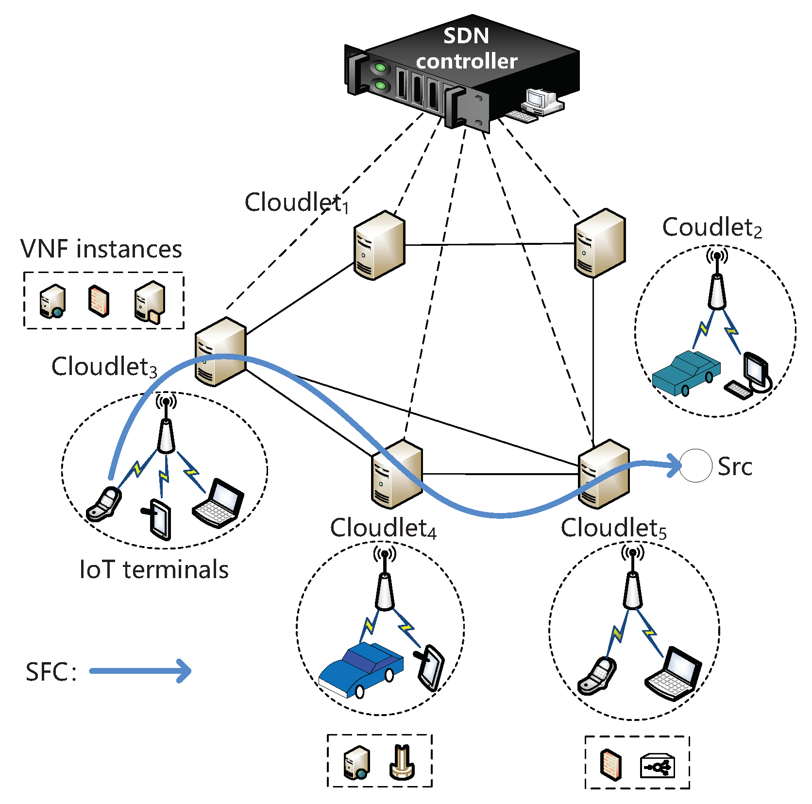
In Figure 1, , an undirected graph is utilized to represent IoT-MEC networks, where represents the set of network nodes and comprises cloudlets () and access point (AP) nodes, while denotes the set of edges. Two nodes, denoted as u and v (), are connected by link (). Due to constrained computational resources in cloudlets, a predetermined quantity of VNFs may be instantiated exclusively within the VMs operating within the cloudlets. The set of all VNF instances is denoted by M in our study. Additionally, is utilized to indicate the set type of VNFs. Each VNF type is indicated by the variable p (), including FW, DPI, load balance, HTTP, etc. The blue line is an example of SFC; when the IoT terminal makes a request, it requires traverse an ordered chain, i.e., SFC, which include a source node; VNFs; and destination node. In the network, APs are in charge of transforming the IoT-SRs to cloudlets, and an SDN controller is used to receive IoT-SRs from APs, i.e., the request from IoT terminals, and placing the SFC. Figure 1 is an example of the network.

Figure 1.
A schematic diagram of IoT-MEC networks.
We use and to denote the CPU capability and process delay of cloudlet c (). The bandwidth capacity, packet loss rate, and delay of link () are represented by , , and , respectively. For each cloudlet (), is used to indicate the count of VNF type p instantiated in c. Furthermore, the availability ratio of CPU for c and the availability ratio of bandwidth for are represented as and , respectively.
3.2. SFC Requests
The set of IoT-SRs is denoted by R. The IoT-SR is denoted by IoT-SR, corresponding to a 7-tuple . In the 7-tuple, and represent the source node and the destination node, respectively. is the set of VNFs requested by IoT-SR in which represent the VNF requirement, and , is the length of IoT-SR, i.e., the total number of VNF instances of IoT-SR. represent the CPU consumption of VNF p, represents the bandwidth consumption of IoT-SR , and and represent the maximum tolerated delay of IoT-SR and the maximum tolerated packet loss rate of IoT-SR, respectively. We use a binary variable () to indicate whether VNF type is deployed on node . Specifically, if there is a VNF instance on the cloudlet node (), equals to 1 and 0 otherwise. Note that we consider the packet loss rate as 0 when a packet traverses across a VNF, since the performance of software and hardware is increasing.
3.3. Problem Description
In IoT-MEC networks, the dynamic SFC placement problem involves looking for or constructing a route path for IoT-SR so that it can minimize the implementation cost based on resource consumption and end-to-end delay of IoT-SR. It is important to emphasize that routing IoT-SRs to cloudlets in close proximity to IoT terminals can effectively reduce end-to-end latency. Since IoT networks change dynamically and IoT-SRs arrive stochastically, the difficulty of dealing with the dynamic SFC placement problem increases, including the placement of VNFs and selection of a traffic path. Based on NFV technology, VNFs can be flexibly and efficiently realized on VMs in the cloudlets. There are usually multiple VNF instances for the same type of VNF in different cloudlets in the network (G), leading to several combinations of candidate VNF instances with different performance for each IoT-SR. To meet the end-to-end delay requirement and efficiently utilize resources, we decompose the dynamic SFC placement problem into two parts: (i) determine the placement of VNFs and (ii) select the optimal path for each adjacent VNF instance pair.
3.4. ILP Model
In this subsection, we formulate the dynamic SFC placement problem as an ILP model.
3.4.1. Resource Constraints
We ensure sufficient cloudlet resources to host VNFs and that the bandwidth of links are sufficient to route traffic for all IoT-SRs (R):
where indicates whether link is traversed by IoT-SR and equals 1 if the traffic of IoT-SR traverses physical link and 0 otherwise.
For each cloudlet, we ensure the following resource constraint:
where is the CPU consumption of VNF type p.
3.4.2. Delay Constraint
We use to denote the delay of IoT-SRi:
where the first part is the processing delay of VNFs type of p on cloudlets (c), which is computed in Equation (5), and the second part is the propagation delay of the links ().
where indicates the processing time required by a cloudlet to handle a unit packet (c) [39].
If an IoT-SR is admitted, its total end-to-end delay in a path cannot exceed the maximum tolerated delay. We use a binary variable () to show whether IoT-SR is accepted or not:
3.4.3. Packet Loss Rate Constraint
This consideration is limited to the packet loss rate on the links, excluding VNF processing. It is required that the selected path for IoT-SR satisfy the constraint on the end-to-end packet loss rate:
where is the packet loss rate of IoT-SR.
As the equation presented above is non-linear, we can linearize it by taking a logarithm on both sides.
3.4.4. Other Constraints
The following equation ensures that the route path for IoT-SR is consecutive and cannot be split:
3.4.5. Optimization Objectives
Finally, we optimize two objectives: the service response delay and resource consumption cost of an IoT-SR. We formulate the resource consumption cost, which consists of VNF placement cost, resource consumption cost, and the penalty for rejecting IoT-SR.
Considering the inflation of marginal costs associated with resource usage as the resource load increases, the relationship between resource utilization and cost is characterized by an exponential function in our study. This relationship can be defined as follows [2]:
In this equation, the constants and are utilized, both of which satisfy the condition . It is worth noting that as the values of and increase, the resource usage cost also increases proportionally.
The placement cost of VNF of type p is formulated as follows:
The activation cost of VNFs of type p is represented as . The selection of cloudlet c by IoT-SR for placement of the required VNF is indicated by the binary variable , which equals 1 if cloudlet c is the node for VNF placement and 0 otherwise.
In the event that the service request of IoT-SR is declined, it incurs a penalty denoted as :
The indicator function () is defined on the basis of set X, that is, if x is true, it equals 1 and and 0 otherwise.
Therefore, the total cost for routing IoT-SR can be represented as follows:
The dynamic SFC placement problem, which aims to minimize the formulation of the weighted sum of the resource consumption cost and the end-to-end delay of every IoT-SR, is expressed as Equation (15):
Parameters and are the weighting coefficients that reflect the importance level of minimizing the delay of forwarding and minimizing the resource consumption cost provisioning of IoT-SR, respectively, where + = 1 and , .
Solving the aforementioned optimization problem with a series of constraints is a non-trivial task, as it has been proven to be NP-hard. Traditional approaches such as ILP solvers or heuristic algorithms require extensive iterations and computations to achieve dynamic VNF placement and traffic routing. In order to address this challenge, we employ an intelligent method known for meta reinforcement learning-based SFC placement (MRL-SFCP) to facilitate real-time network transitions and optimize the placement of dynamic SFCs.
4. Dynamic Placement of SFC Based on Meta Reinforcement Learning and Fuzzy Logic
In this section, we first provide an overview of the proposed solution and describe the Markov property of the dynamic IoT-MEC networks. Then, we formulate the problem as an MDP model, which is defined as a triple . Finally, we describe the MRLF-SFCP in stages in detail.
4.1. Overview
As IoT-MEC scenarios are rapidly changing and often affected by many factors and traditional intelligent schemes cannot adapt to changes in the environment and need to retrain the neural network, we utilize meta reinforcement learning to tackle the above challenges. It comprises an outer model and a inner model. The former is used to learn the initial parameters of the inner model. When the environment undergoes changes, such as variations in cloudlet performance or link bandwidth, the parameters of the neural network in the inner model can be adjusted by the outer model. The latter uses DDQN and fuzzy logic to realize an SFC placement decision model by receiving the SFCRs and initial parameters.
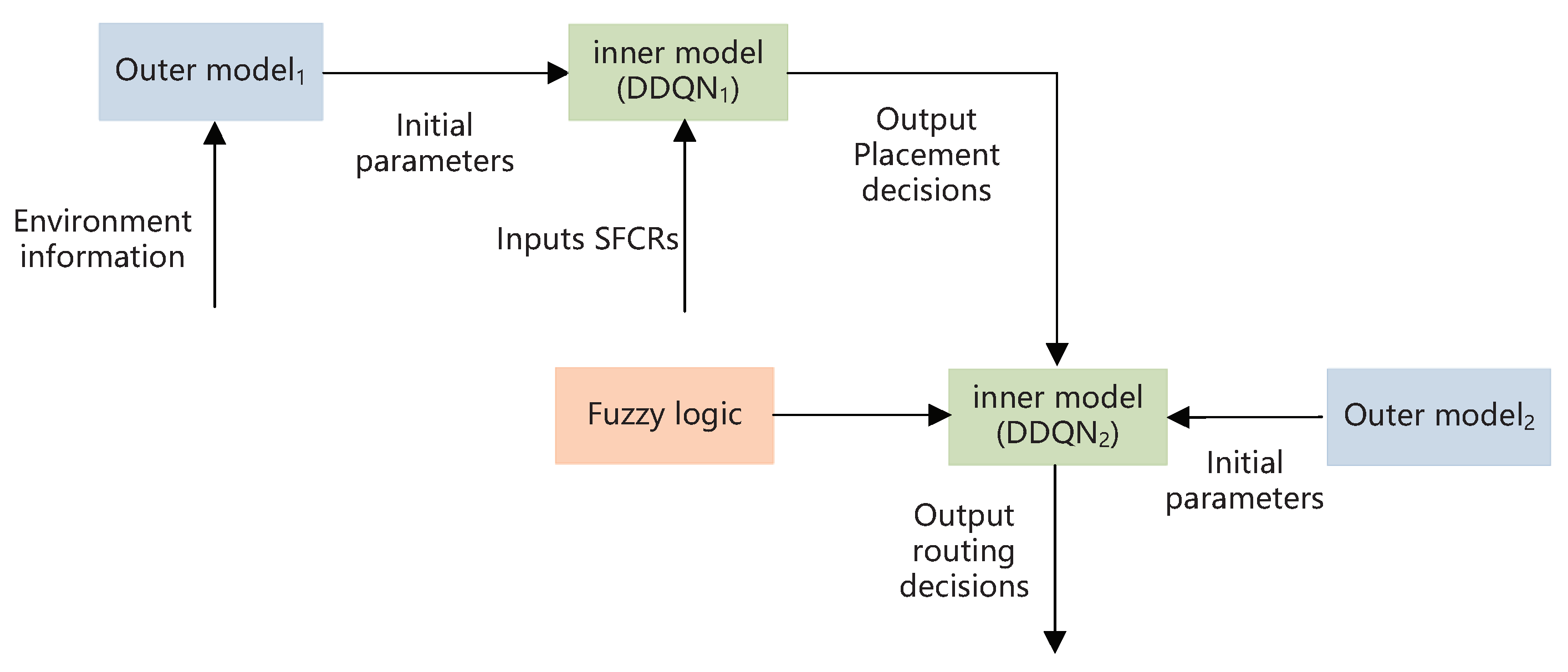
Figure 2 shows an illustration of the MRLF-SFCP. is used to adjust the parameters of the VNF placement neural network. is used to adjust the parameters of the traffic routing neural network. To achieve optimal SFC placement, first, we use to acquire the initial parameters of neural network. Then, the optimal combination of VNF instances is acquired using (DDQN1). Subsequently, a verification is conducted to ascertain the placement status of the necessary VNF instances on the designated cloudlets. If the required VNF instances do not exist, they are dynamically placed onto the corresponding cloudlets. Then, we utilize to acquire the initial parameters of (DDQN2). Additionally, to establish connectivity between the source and destination node, as well as the selected cloudlets generated by (DDQN1), MRLF-SFCP employs fuzzy logic for preliminary link evaluation and utilizes the DDQN algorithm to determine the optimal route. For instance, in Figure 1, there are four paths that need to be produced in a predefined order, namely, (IoT terminal, ), (, ), (, ), and (, src). We need to perform fuzzy logic and DDQN four times for traffic routing. In particular, the evaluation of link quality, considering factors such as available bandwidth, link and node delays, and packet loss rate, is performed using fuzzy logic. The evaluation result is input to (DDQN2) for routing selection.
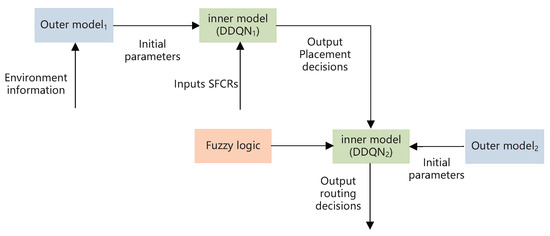
Figure 2.
A framework for placing dynamic SFCs based on meta reinforcement learning and fuzzy logic.
4.2. MDP Model
In a real network scenario, it is difficult to find an optimal routing path in a dynamic network as a result of the changing of the network and the stochastic arrival of IoT-SRs. The next SFC placement is only relevant to the state of the network at the moment. Thus, we can use an MDP model to model the dynamic network.
First, we depict the input of the VNF placing network, i.e., the network state (), which includes the following several elements:
- The ratio of the remaining CPU resource in the cloudlets , where is the cardinality of set ;
- The CPU resource consumption () of VNF type of IoT-SR;
- The requirement for end-to-end delay () of IoT-SR;
Subsequently, a vector can be utilized to characterize the network state :
The input of SPFN is described as follows:
- The ratio of the remaining bandwidth in the links is , where is the number of links in IoT-MEC networks;
- Binary codes are used to represent the path in IoT-SR: , where . These codes encode the node location information using binary coding. For instance, when considering a network comprising 60 nodes and assuming the second node as the source node and the fifteenth node as the destination node, their binary codes would be and , respectively. The length of the binary code a is ;
- The bandwidth requirement of IoT-SR: ;
- The requirement for end-to-end delay in IoT-SR: .
- The maximum tolerated packet loss rate of IoT-SR: .
Consequently, a vector formulation can be used to represent the network state :
Second, the definition of the action space is presented.
The action set () is defined as the collection of all possible combinations of cloudlets. Specifically, in IoT-MEC networks with N cloudlets and an IoT-SR requiring traversal of K types of VNF instances, the task involves selecting three VNF instances among the N cloudlets. Once an action is chosen, we must check whether there is a corresponding VNF instance on the cloudlet; if not, the VNF instance is dynamically placed immediately.
Subsequently, the action is denoted as the pathway employed to establish connectivity between the initial and terminal nodes. Since paths needed to be generated to connect the source and destination nodes and the nodes chosen by the VNF placing network in predefined order, the agent, i.e., (DDQN2), must determine the path iteratively.
Third, the reward function of the VNF placing network is defined as follows:
The selected set of cloudlets, denoted as , holds significance in the formulation of the reward function. In order to maintain algorithm stability, scaling factors and are employed to equalize the magnitudes of the two rewards.
Prior to computing the reward based on the given state and selected action, it is necessary to assess whether the chosen cloudlets possess adequate resources to accommodate VNF placement. If sufficient resources are available, the reward is calculated using Equation (18); otherwise, the reward is set to . Thus, the agent would attempt to select the cloudlet with the highest remaining resource ratio to enhance the acceptance rate of IoT-SRs.
Finally, our objective is to jointly optimize the cost of resource usage and end-to-end delay. To achieve this objective, the reward function of the SPFN is formulated as the negative weighted summation of the cost associated with resource consumption and the delay experienced in end-to-end communication. When there is no practicable path for IoT-SR, the reward of SPFN remains consistently fixed at and can be formulated as follows:
The path set () represents the collection of paths that establish connections among the initial node, the terminal node, and the chosen cloudlets. To maintain algorithm stability, we introduce weighted factors and to ensure comparable magnitudes between the two rewards. Since is a small value relative to the resource consumption cost on the link, it is necessary to ensure that is greater than to ensure stable training.
4.3. Fuzzy Logic
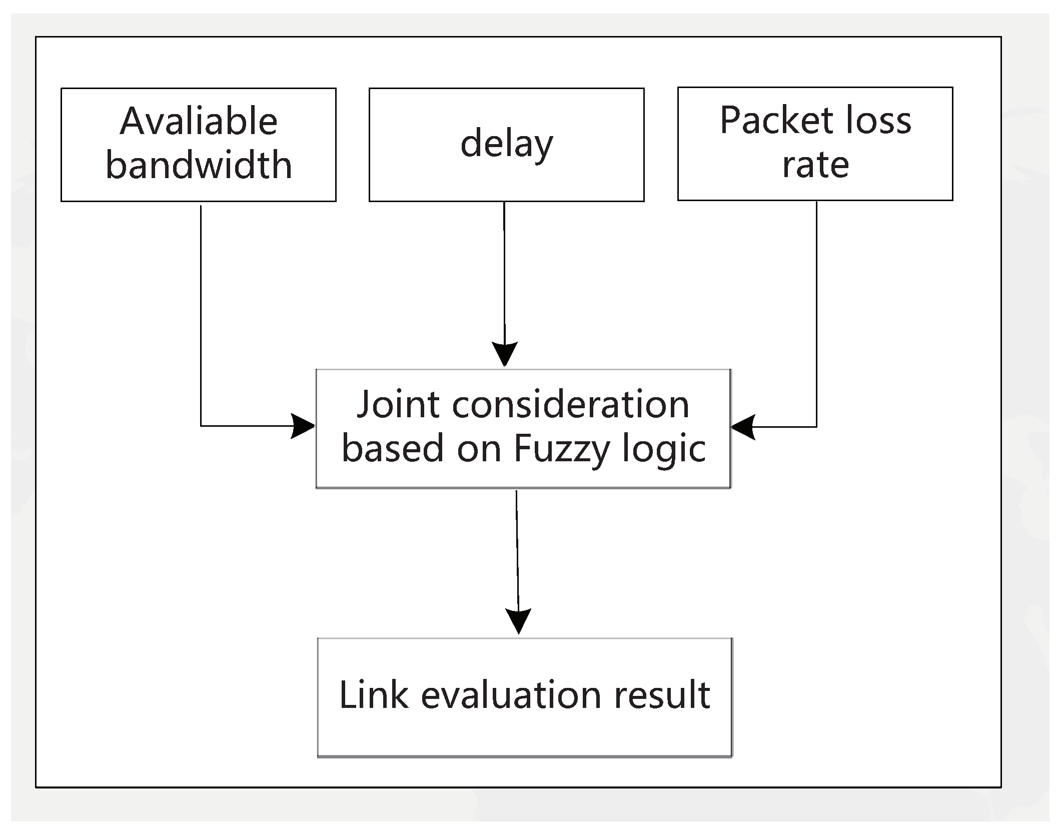
In classical Boolean logic, “false” is usually denoted by 0, and “true” is denoted by 1; a proposition is either true or false. In fuzzy logic, a proposition is no longer either true or false; it can be thought of as “partially true”. Fuzzy logic uses non-numeric linguistic variables to express facts and further deals with approximate data in a manner similar to human reasoning. It comprises three main procedures (see Figure 3): first, convert the input values to fuzzy values, i.e., fuzzification. The degree to which the bandwidth of a link is part of the large, medium, and small categories is calculated using the bandwidth membership function. Similarly, the degree to which the delay belongs to the large, medium, and small categories and the degree to which the packet loss rate belongs to the large, medium, and small categories need to be calculated using the corresponding membership function. Then, IF/THEN rules are used to obtain the fuzzy output values. Those fuzzy output values are defined as fire strength (FS) and cannot solve real problems. Therefore, defuzzification can be used to obtain certain numerical values and set a threshold () for evaluation of links.
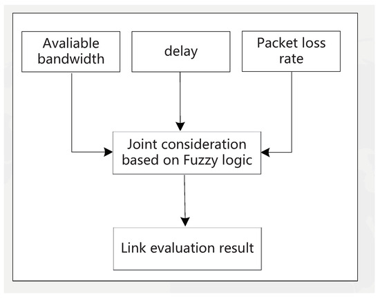
Figure 3.
The procedure of link evaluation.
4.4. Outer Model
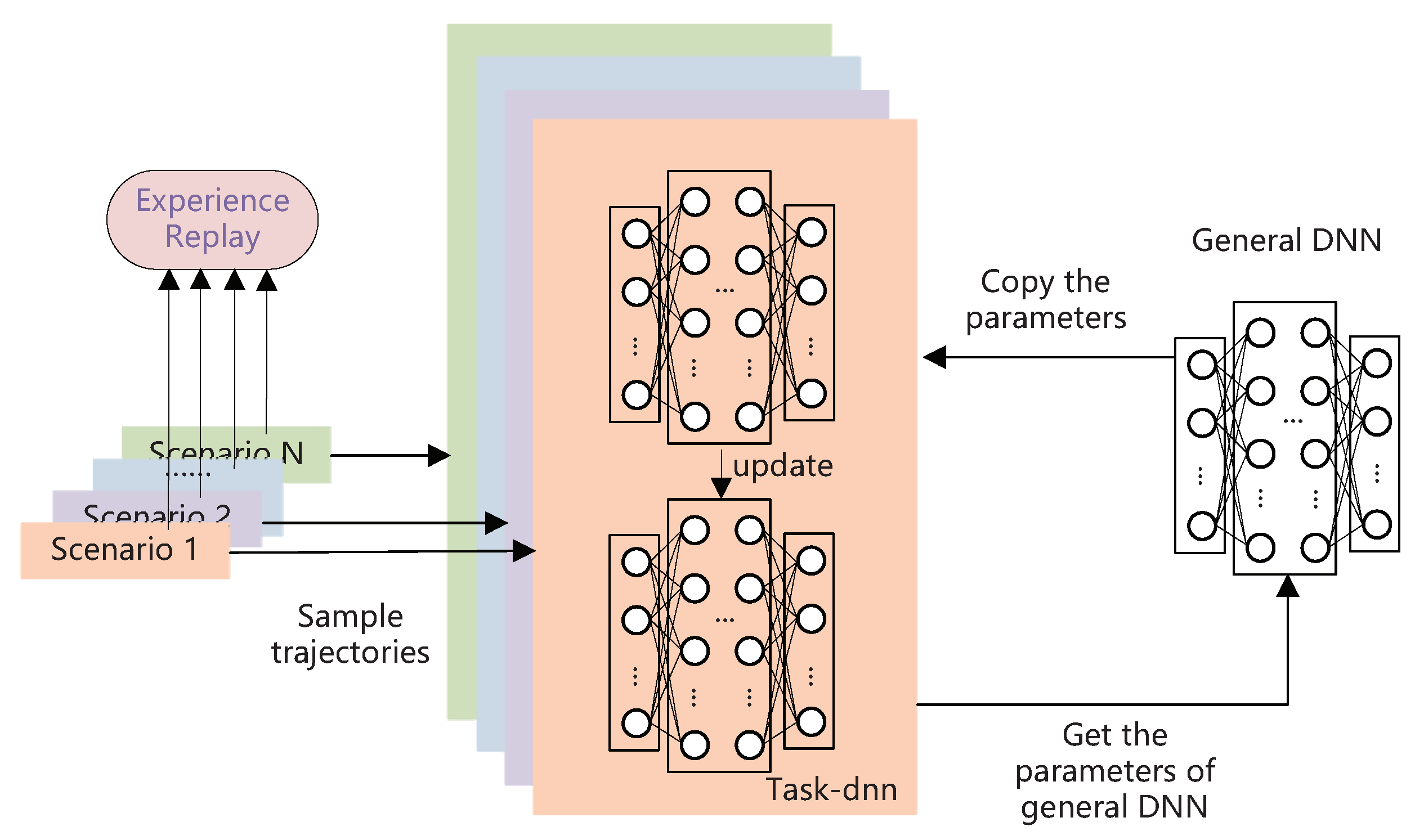
The general training process of the outer model is depicted in Figure 4. We can see that the acquisition of initial parameters includes the training of the task DNN and the training of the general DNN. The former entails conducting step-by-step optimization training for each scenario, while the latter involves periodically synchronizing updates on a batch of sampled scenarios. Specifically, we randomly select some IoT-MEC scenarios. For each chosen IoT-MEC scenario, we copy a general DNN named the task DNN and train it with a batch of trajectories randomly sampled from experience replay. In other words, the parameter update of each task DNN is performed based on the globally shared initialization of parameters that are inherited. After the completion of network parameter updates for each trajectory in the batch, the adapted policy’s capability for each IoT-MEC scenario can be evaluated by calculating the loss function of the query set. And the calculated loss functions are used to optimize the general DNN parameters. After completing the iteration over all selected IoT-MEC scenarios, the general DNN parameter is updated to incorporate the learning experience gained from policies associated with known learning scenarios. The algorithmic process of meta learning is shown in Algorithm 1.
| Algorithm 1 The general training process of the outer model |
| Require: Different IoT-MEC scenarios, iteration times N |
| Ensure: Trained general DNN model with better initial parameters which used in inner model |
|
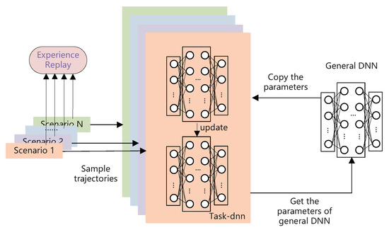
Figure 4.
The general training process of outer model.
4.5. Inner Model
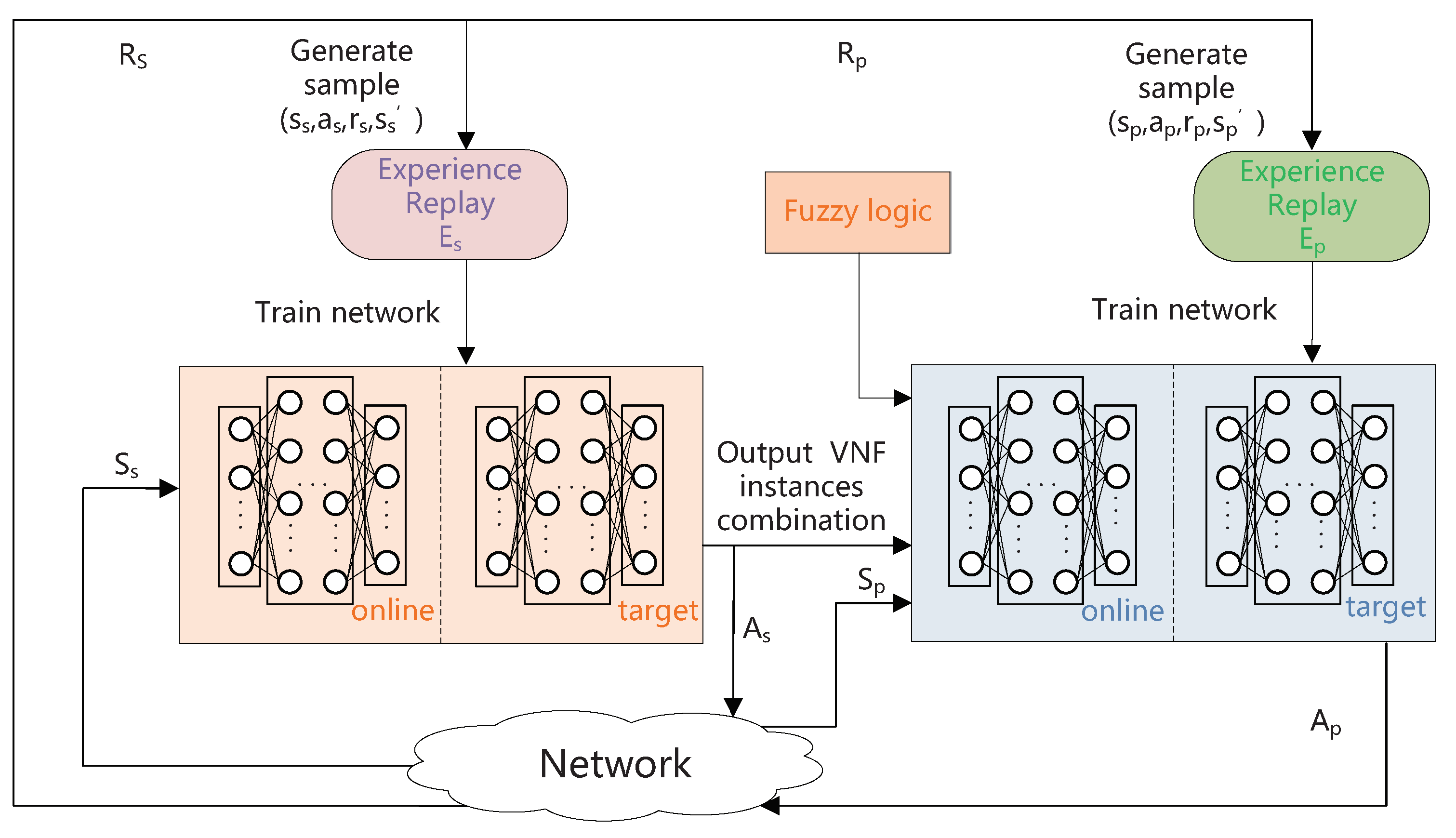
Figure 5 shows an illustration of the proposed DDQN-based inner model. After we obtain the optimal initial parameters of the inner model, we can use them to train the inner model, which is directed at the new running IoT-MEC scenario. The inner model is used to make the placement and routing decisions.

Figure 5.
Dynamic SFC placement framework based on DDQN.
In this paper, a neural network is utilized to approximate the value function. The distribution of the Q function can be approximated more precisely and achieve an effective SFC placement strategy through continuous training of the DDQN network. The experience replay pool is employed by the DDQN network to store empirical samples from each iteration, and network parameters are updated by randomly extracting data from the experience replay pool. This approach helps to break the correlation between data. As we use the DDQN model to solve the two subproblems, i.e., the VNF placing network and SPFN, we use a similar method to train the neural network for both. First, the parameters of the neural network of the inner model are initialized as the parameters of the trained general network. The agent interacts with the environment to generate trajectories stored in experience memory. Then, we extract a batch of trajectories to train the neural network of the inner model, which aims at achieving fast adaptation in the current IoT-MEC scenario within a few steps. Finally, we can use the trained inner model to make the placement/routing decisions. We present the algorithmic process of meta adapting in Algorithm 2.
| Algorithm 2 Meta adaption procedure |
|
After training the neural network, we can use the trained model to realize dynamic SFC placement in IoT-MEC networks, which can be broken down into three stages: (1) Acquire the current network state using the SDN controller and send it to the agent; then, use to select the optimal combination of VNF instances, i.e., determine the cloudlets for IoT-SRs to traverse. Then, dynamically place VNF instances according to the action with the highest reward. (2) Conduct a preliminary evaluation of each link by considering available bandwidth, delay, and packet loss rate using fuzzy logic. (3) Choose the top k links in terms of performance and use to further choose the routing action with the highest reward based on the output of and the current state (). The pseudocode of the online running algorithm is depicted in Algorithm 3.
| Algorithm 3 Running algorithm of MRLF-SFCP |
| Require: VNF placing network: ; |
| The network for searching SFC path: ; |
| Remaining resource ratios: |
| and ; |
| IoT-SRs set R. |
| Ensure: The routing path of IoT-SR which is denoted as . |
|
5. Performance Evaluation
5.1. Simulation Settings
5.1.1. Topology Settings
As a consequence of the heterogeneous and stochastic placement characteristics of IoT equipment, the IoT-MEC network’s actual topology is irregular. To address this, we employ the NetworkX3.1 [40] library to construct three representative network topologies for simulation purposes in our study. The utilization of this approach facilitates the demonstration of the suitability and universality of the MRL-SFCP algorithm. Within the scope of this investigation, the network topologies include a random network (RN), small-world network (SWN) [41], and scale-free network (SFN) [42], correspondingly. Amongst each category of network topology, a total of 24 nodes exist, of which 8 nodes are designated as cloudlets, which are primarily utilized to execute IoT-SRs by employing placed VNFs. Additionally, the RN has a connectivity probability of 0.4, the SWN has 10 neighbor nodes and a reconnect probability of 0.2, and the SFN consists of an initial node count of 7.
We consider six types of VNFs: firewall, proxy, NAT, IPS, IDS, and gateway, with CPU requirements of 1600 MIPS, 1200 MIPS, 2000 MIPS, 3000 MIPS, 2400 MIPS, and 1800 MIPS, respectively [2]. Each cloudlet is placed with one or two types of VNF instances, and IoT-SRs are randomly produced in AP nodes. We set the CPU capacity of each cloudlet within the range of 3000 to 8000 MIPS. The bandwidth and delay of each link are set within the ranges of [1000, 10,000] Mbps and [2, 5] ms, respectively. For the sake of simplifying the problem, the delay on cloudlets is randomly set from 4 to 8 ms. We set the weighted factors in Equation (19), i.e., and , as 3 and 1, respectively.
5.1.2. SFC Request
In this paper, it is assumed that each IoT-SR must pass through three types of VNFs before reaching the destination node [8]. The bandwidth requirement () for each IoT-SR is randomly set within the range of [10, 120] Mbps. The maximize tolerated delay () is set within the range of [50, 100] ms.
5.1.3. Comparison Methods
- Random: The random algorithm stochastically chooses cloudlets to place/traverse VNF instances and routing paths to connect two adjacent VNF instances for every incoming IoT-SR;
- DLG [43]: For each arrived IoT-SR, the delay-least-greedy (DLG) method is commonly employed to select cloudlets and the paths that exhibit the minimum delay. Simultaneously, an enhancement is made to this method by assigning a high cost to cloudlets and links with high loads, thereby preventing their selection;
- DDQN-SP: This algorithm utilizes the DDQN algorithm to select cloudlets and the Dijkstra algorithm to search the routing path for each IoT-SR;
- DLA-DVPRP [2]: This algorithm utilizes the shortest path algorithm based on the Lagrange relaxation method to solve the delay and packet loss aware dynamical VNF placement and routing problem (DLA-DVPRP) for SFC requests. We modify it to adapt to IoT-SR in the dynamic IoT-MEC network.
5.1.4. Simulation Platform
The simulation environment is set up on a machine with an Intel Core i5 and 16 GB RAM. We use a Python-based framework and Tensorflow to build and train deep neural networks and improve the following comparison algorithms. Since our method is based on reinforcement learning, there is no need for an initial dataset. In practical scenarios, Ryu is selected as the SDN controller and is deployed in a docker container in the central cloud server. K8s is used as the container orchestrator in the central cloud. The VNFs are deployed in the docker containers of MEC. Kubeedge is used as a container orchestrator in MECs. Our proposed algorithm, MRL-SFCP, is deployed in SDN controllers to execute scheduling.
5.2. Results and Discussion
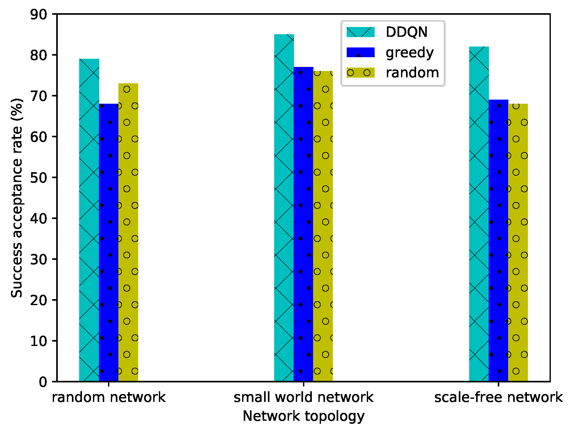
We first use the trained VNF placing network to choose cloudlets for arrived IoT-SRs online. In order to evaluate the performance of the VNF placing network, simulations are carried out across three distinct network topologies, specifically RN, SWN, and SFN. In this experiment, we mainly compare the performance of three types of algorithms, namely machine learning algorithm DDQN, a greedy algorithm, and a random algorithm. When required VNFs of IoT-SR are not in the chosen cloudlets and there are insufficient resources to place VNF instances, we label the IoT-SR as "cannot be accepted" and set the reward as −200 directly. The simulation result is obtained by randomly setting CPU and bandwidth resources, and the average value of twenty experiments is taken into consideration. The success acceptance rate of IoT-SRs in various topologies is illustrated in Figure 6. It is evident from the results that the DDQN algorithm consistently attains the highest traffic acceptance rate. The the average acceptance rate of IoT-SRs using the DDQN algorithm across the three networks is 18.4% higher than that of the random method and 20.8% higher than that of the DLG.
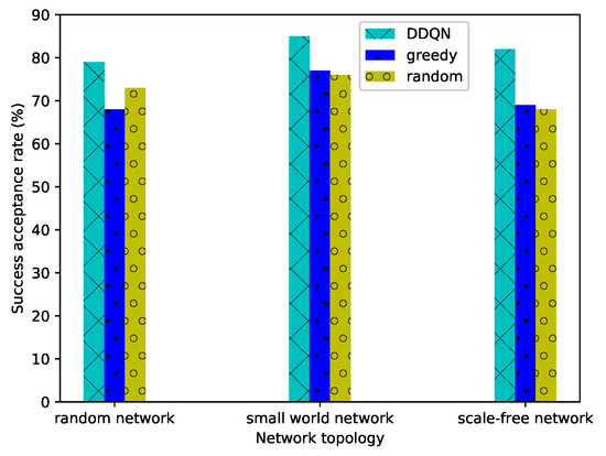
Figure 6.
The acceptance rate in different network topologies.
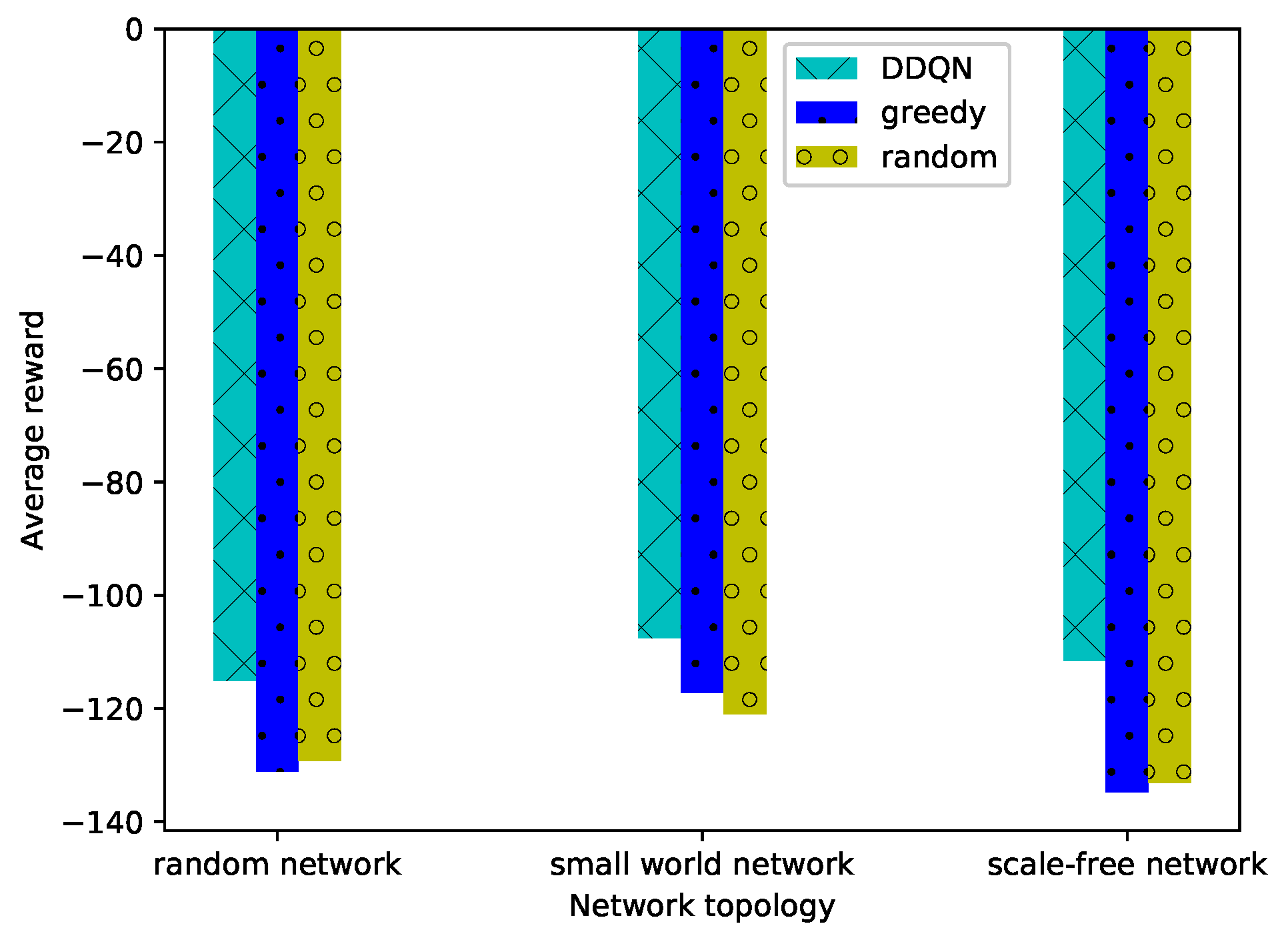
Figure 7 presents the average rewards of IoT-SRs under three networks. The simulation results demonstrate that under all network topologies, our proposed DRL-based method outperforms the other approaches by a significant margin. In most cases, the performance of the greedy method is inferior to that of the random method, as it always chooses the cloudlets with the lowest delay, easily making the resources of some cloudlets become very small after a number of IoT-SRs, while the random method selects all cloudlets with equal probabilities for each IoT-SR.

Figure 7.
The average reward of IoT-SRs in different network topologies.
In Figure 8, an evaluation is conducted to compare the traffic acceptance rate within the RN topology. The IoT-SRs arrive at IoT-MEC networks randomly, and the required resources can be acquired only when they come into the network. The results indicate that in the majority of cases, MRL-SFCP exhibits superior performance compared to the other approaches. This finding signifies that the trained agent effectively guides the SDN controller in dynamically placing VNFs and identifying appropriate route paths. Additionally, with an increase in the number of IoT-SRs, as the DLG and random methods cannot dynamically place VNFs and they may fail to discover paths capable of serving IoT-SRs, they achieve poor performance. The DLA-DVPRP uses heuristic algorithms for path selection, achieving lower performance than MRL-SFCP and DDQN-SP. However, since the DLA-DVPRP can dynamically place VNFs, its performance is higher than that of the DLG and random methods.
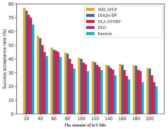
Figure 8.
The acceptance rate of IoT-SRs of the RN.
To facilitate a comprehensive understanding of the experimental findings, Figure 9 shows the mean reward of IoT-SRs in the RN. The defined reward in this study is comprised of the weighted summation of resource utilization cost and delay, aligning with our optimization goals. It is evident that the DDQN-SP surpasses the compared approaches solely when the count of IoT-SRs is less than 35. When the number of IoT-SRs is greater than 40, a noticeable and rapid decline is observed. Conversely, the proposed MRL-SFCP algorithm demonstrates minimal variation and achieves the highest reward. Based on these observations, it can be inferred that the performance of the MRL-SFCP algorithm surpasses that of other methods within the RN topology.
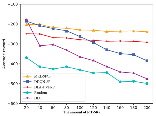
Figure 9.
The mean reward of IoT-SRs within the RN.
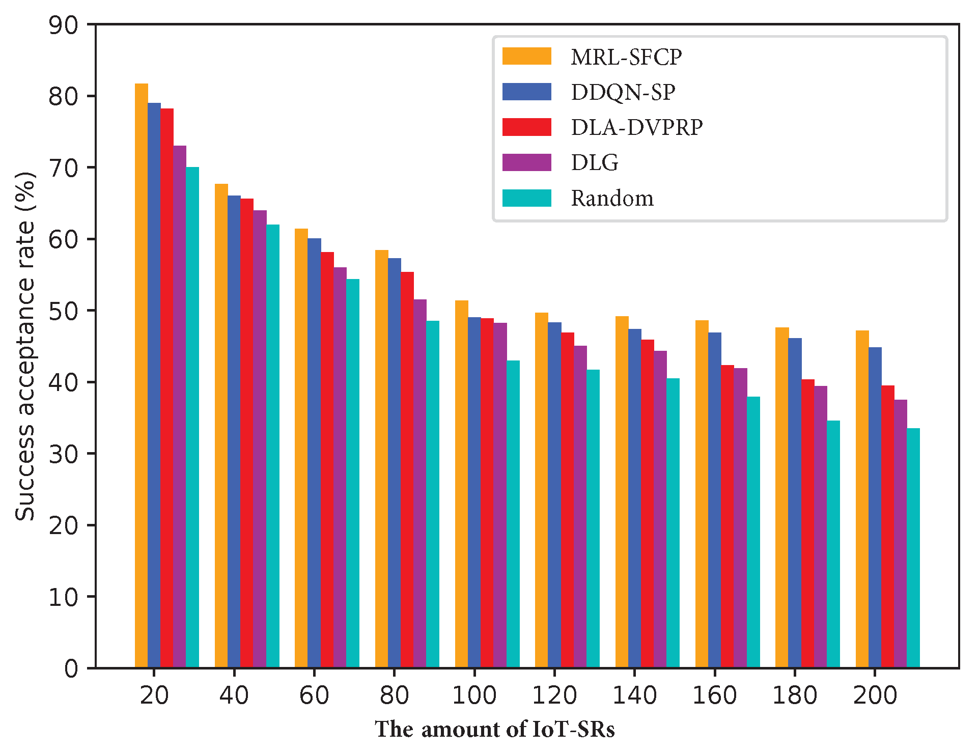
In this study, we compare the acceptance rate of IoT-SRs obtained through the MRL-SFCP approach with that obtained using alternative methods. Figure 10 presents the traffic acceptance rate of different algorithms from the SWN topology while varying the number of IoT-SRs from 20 to 200. We can observe that there is a small performance difference between DDQN-SP and the proposed MRL-SFCP algorithm, since they use DRL to place VNF instances and the IoT-SRs are be rejected when there is no path for route traffic or the selected path has insufficient resources. The results demonstrate the consistent superiority of the acceptance rate of IoT-SRs achieved using the proposed MRL-SFCP algorithm in comparison to the other algorithms under investigation.
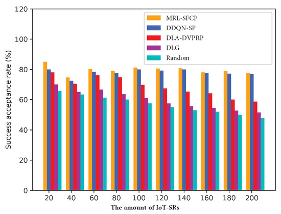
Figure 10.
The acceptance rate of IoT-SRs in the SWN.
The average reward of IoT-SRs in the SWN topology is illustrated in Figure 11 as the number of IoT-SRs varies from 20 to 200. It can be observed that the MRL-SFCP algorithm attains the highest reward after 80 IoT-SRs. This phenomenon can be attributed to the consistent identification of the shortest path by DDQN-SP, rendering it well-suited for scenarios featuring a limited number of IoT-SRs. Nonetheless, as the number of IoT-SRs escalates, the DDQN-SP struggles to maintain a balanced utilization of network resources. This causes a rapid decline in the average reward after 80 IoT-SRs. The three other compared methods exhibit similar phenomena after 80 IoT-SRs. Based on the results obtained in the SWN, the proposed MRL-SFCP algorithm exhibits superior performance.
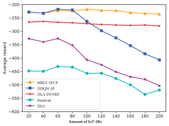
Figure 11.
Average reward of IoT-SRs in the SWN.
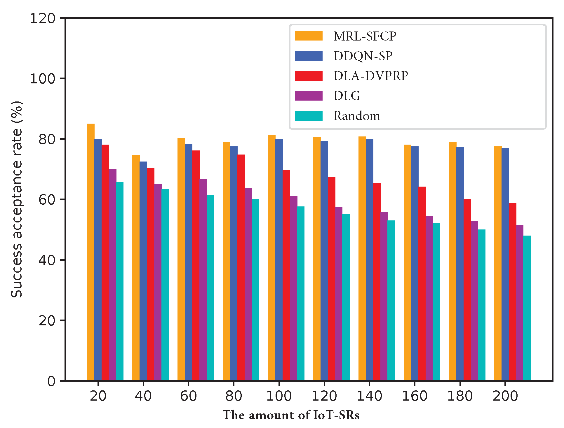
Figure 12 illustrates the acceptance rate of IoT-SRs within the SFN topology, showing that both our proposed MRL-SFCP and DDQN-SP obtain the highest traffic acceptance rate of IoT-SRs in comparison to other methods. With the number of IoT-SRs increasing, the acceptance rate of IoT-SRs shows a significant decrease across all investigated algorithms. This decline is attributed to the increased resource consumption costs and the emergence of bottleneck links and cloudlets. Furthermore, we can observe that the result for all algorithms exhibits the same trend as the aforementioned network.

Figure 12.
Success acceptance rate of IoT-SRs in the SFN.
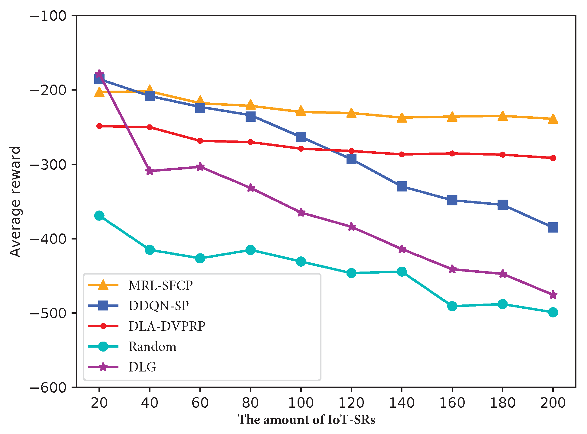
The average reward of IoT-SRs is presented in Figure 13 for the SFN topology, considering a range of 20 to 200 IoT-SRs. It can be observed that all the methods exhibit a similar changing trend in terms of average reward, aligning with the aforementioned network characteristics. We can observe that our proposed MRL-SFCP algorithm achieves greater rewards than the other methods for a large number of IoT-SRs and the best traffic acceptance rate of IoT-SRs in most cases. In this work, the resource demands of IoT-SRs are constantly changing, which results in a dynamic scenario. Hence, the incorporation of dynamic SFC placement strategies becomes essential in minimizing the weighted sum of resource utilization cost and end-to-end latency. The outcomes highlight the adaptability to network changes and indicate the efficiency of resource utilization of the proposed MRL-SFCP algorithm.
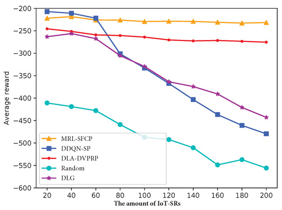
Figure 13.
Average reward of IoT-SRs in the SFN.
In view of the experimental analyses under different network topologies presented above, we only conduct an experiment on the SFN topology to compare the accepted traffic throughput. Table 2 shows the throughput corresponding with 100, 150, and 200 IoT-SRs. When the number of IoT-SRs is 150, we can see that the throughput of our proposed MRL-SFCP algorithm is about 1 Gbp higher than that of DDQN-SP, 1.6 Gbps higher than that of DLA-DVPRP, 2 Gbps higher than that of DLG, and 4.7 Gbps higher than that of the random method because DDQN-SP, DLG, and the random method cannot ensure link load balancing. Although the DLA-DVPRP algorithm takes into account load balancing for links and nodes, its performance is not as good as that of MRL-SFCP and DDQN-SP, which consider both link delay and link jitter when searching for routing paths for IoT-SR.
Table 2.
The accepted traffic throughput of IoT-SRs in the SFN.
In order to present the computational efficiency of these algorithms, we compare them in terms of running times. Table 3 illustrates that MRL-SFCP has a significantly lower running time in comparison with other algorithms. In larger networks, traditional methods encounter significant time complexity when searching for optimal VNF placement strategies and performing routing path selection. DDQN-SP exhibits slightly longer running times compared to MRL-SFCP, which is attributed to the use of the shortest path algorithm for routing.
Table 3.
Running times of different schemes.
6. Conclusions
In this paper, an efficient algorithm named MRL-SFCP is proposed to address the SFC placement problem posed by IoT-SRs in dynamic IoT-MEC networks. The SFC placement problem is first decomposed two subproblems—VNF placement and traffic routing—and is then modeled as an MDP involving the environmental state, action space, and reward function. To capture real-time network fluctuations, two types of DDQN networks—an VNF placing network and an SFC path finding network—are specifically designed to facilitate optimal selection of VNF instances and determination of routing paths. We then propose a meta reinforcement learning-based SFC placement (MRL-SFCP) policy that integrates meta reinforcement learning and fuzzy logic to address the dynamic SFC placement problem. According to the simulation results, the proposed method demonstrated remarkable performance superiority according to traffic throughput, acceptance rate, and average reward of IoT-SFCRs in comparison to other baseline methods across three representative network topologies. In this paper, we assume that each IoT-SR only passes through three types of VNFs before reaching the destination node. There are certain limitations, and future research will further improve the proposed algorithm to adapt to any length of SR, enhance the capabilities of the agent, and expand the scalability and adaptability of MRL-SFCP to accommodate networks of varying scales.
Author Contributions
Conceptualization, S.G. and Y.D.; methodology, S.G. and Y.D.; software, Y.D.; validation, S.G. and Y.D.; formal analysis, S.G.; investigation, S.G.; resources, S.G.; data curation, Y.D.; writing—original draft preparation, S.G. and Y.D.; writing—review and editing, Y.D. and L.L.; visualization, L.L.; supervision, S.G. and L.L.; project administration, S.G.; funding acquisition, S.G. and L.L. All authors have read and agreed to the published version of the manuscript.
Funding
This research was funded by the Science and Technology Research Youth Project of Chongqing Municipal Education Commission under Grant KJQN202202401, Chongqing University of Posts and Telecommunications Doctoral Initiation Foundation (A2023007).
Institutional Review Board Statement
Not applicable.
Informed Consent Statement
Not applicable.
Data Availability Statement
Not applicable.
Conflicts of Interest
The authors declare no conflict of interest.
References
- An, X.; Fan, R.; Hu, H.; Zhang, N.; Atapattu, S.; Tsiftsis, T.A. Joint Task Offloading and Resource Allocation for IoT Edge Computing with Sequential Task Dependency. IEEE Internet Things J. 2022, 9, 16546–16561. [Google Scholar]
- Liu, L.; Guo, S.; Liu, G.; Yang, Y. Joint Dynamical VNF Placement and SFC Routing in NFV-Enabled SDNs. IEEE Trans. Netw. Serv. Manag. 2021, 18, 4263–4276. [Google Scholar] [CrossRef]
- Sun, J.; Zhang, Y.; Liu, F.; Wang, H.; Xu, X.; Li, Y. A survey on the placement of virtual network functions. J. Netw. Comput. Appl. 2022, 202, 103361. [Google Scholar]
- Masoudi, R.; Ghaffari, A. Software defined networks: A survey. J. Netw. Comput. Appl. 2016, 67, 1–25. [Google Scholar]
- Li, J.; Liang, W.; Huang, M.; Jia, X. Reliability-Aware Network Service Provisioning in Mobile Edge-Cloud Networks. IEEE Trans. Parallel Distrib. Syst. 2020, 31, 1545–1558. [Google Scholar] [CrossRef]
- Oikonomou, E.; Rouskas, A. Optimized Cloudlet Management in Edge Computing Environment. In Proceedings of the 2018 IEEE 23rd International Workshop on Computer Aided Modeling and Design of Communication Links and Networks (CAMAD), Barcelona, Spain, 17–19 September 2018; pp. 1–6. [Google Scholar]
- Liu, Y.; Lu, H.; Li, X.; Zhang, Y.; Xi, L.; Zhao, D. Dynamic Service Function Chain Orchestration for NFV/MEC-Enabled IoT Networks: A Deep Reinforcement Learning Approach. IEEE Internet Things J. 2021, 8, 7450–7465. [Google Scholar] [CrossRef]
- Pei, J.; Hong, P.; Pan, M.; Liu, J.; Zhou, J. Optimal VNF Placement via Deep Reinforcement Learning in SDN/NFV-Enabled Networks. IEEE J. Sel. Areas Commun. 2020, 38, 263–278. [Google Scholar]
- Tomassilli, A.; Giroire, F.; Huin, N.; Pérennes, S. Provably Efficient Algorithms for Placement of Service Function Chains with Ordering Constraints. In Proceedings of the IEEE Conference on Computer Communications (IEEE INFOCOM), Honolulu, HI, USA, 16–19 April 2018; pp. 774–782. [Google Scholar]
- Pei, J.; Hong, P.; Xue, K.; Li, D. Efficiently Embedding Service Function Chains with Dynamic Virtual Network Function Placement in Geo-Distributed Cloud System. IEEE Trans. Parallel Distrib. Syst. 2019, 30, 2179–2192. [Google Scholar]
- Chen, Y.R.; Rezapour, A.; Tzeng, W.G.; Tsai, S.C. RL-Routing: An SDN Routing Algorithm Based on Deep Reinforcement Learning. IEEE Trans. Netw. Sci. Eng. 2020, 7, 3185–3199. [Google Scholar]
- Yang, S.; Li, F.; Trajanovski, S.; Chen, X.; Wang, Y.; Fu, X. Delay-Aware Virtual Network Function Placement and Routing in Edge Clouds. IEEE Trans. Mob. Comput. 2021, 20, 445–459. [Google Scholar]
- Jin, P.; Fei, X.; Zhang, Q.; Liu, F.; Li, B. Latency-aware VNF Chain Deployment with Efficient Resource Reuse at Network Edge. In Proceedings of the IEEE Conference on Computer Communications (IEEE INFOCOM), Toronto, ON, Canada, 6–9 July 2020; pp. 267–276. [Google Scholar]
- Jia, J.; Yang, L.; Cao, J. Reliability-aware Dynamic Service Chain Scheduling in 5G Networks based on Reinforcement Learning. In Proceedings of the IEEE Conference on Computer Communications (IEEE INFOCOM), Vancouver, BC, Canada, 10–13 May 2021; pp. 1–10. [Google Scholar]
- Feriani, A.; Wu, D.; Xu, Y.T.; Li, J.; Jang, S.; Hossain, E.; Liu, X.; Dudek, G. Multiobjective load balancing for multiband downlink cellular networks: A meta-reinforcement learning approach. IEEE J. Sel. Areas Commun. 2022, 40, 2614–2629. [Google Scholar]
- Zhao, M.; Abbeel, P.; James, S. On the effectiveness of fine-tuning versus meta-reinforcement learning. Adv. Neural Inf. Process. Syst. 2022, 35, 26519–26531. [Google Scholar]
- Bing, Z.; Lerch, D.; Huang, K.; Knoll, A. Meta-reinforcement learning in non-stationary and dynamic environments. IEEE Trans. Pattern Anal. Mach. Intell. 2022, 45, 3476–3491. [Google Scholar]
- Ding, X.; Zhang, Y.; Li, J.; Mao, B.; Guo, Y.; Li, G. A feasibility study of multi-mode intelligent fusion medical data transmission technology of industrial Internet of Things combined with medical Internet of Things. Internet Things 2023, 21, 100689. [Google Scholar]
- Lu, Z.; Cheng, R.; Jin, Y.; Tan, K.C.; Deb, K. Neural architecture search as multiobjective optimization benchmarks: Problem formulation and performance assessment. IEEE Trans. Evol. Comput. 2023. [Google Scholar] [CrossRef]
- Liu, Y.; Pei, J.; Hong, P.; Li, D. Cost-Efficient Virtual Network Function Placement and Traffic Steering. In Proceedings of the ICC 2019—2019 IEEE International Conference on Communications (ICC), Shanghai, China, 20–24 May 2019; pp. 1–6. [Google Scholar]
- Pei, J.; Hong, P.; Xue, K.; Li, D. Resource Aware Routing for Service Function Chains in SDN and NFV-Enabled Network. IEEE Trans. Serv. Comput. 2021, 14, 985–997. [Google Scholar]
- Gu, L.; Hu, J.; Zeng, D.; Guo, S.; Jin, H. Service Function Chain Deployment and Network Flow Scheduling in Geo-Distributed Data Centers. IEEE Trans. Netw. Sci. Eng. 2020, 7, 2587–2597. [Google Scholar]
- Poularakis, K.; Llorca, J.; Tulino, A.M.; Taylor, I.; Tassiulas, L. Joint Service Placement and Request Routing in Multi-cell Mobile Edge Computing Networks. In Proceedings of the IEEE Conference on Computer Communications (IEEE INFOCOM), Paris, France, 29 April–2 May 2019; pp. 10–18. [Google Scholar]
- Behravesh, R.; Harutyunyan, D.; Coronado, E.; Riggio, R. Time-Sensitive Mobile User Association and SFC Placement in MEC-Enabled 5G Networks. IEEE Trans. Netw. Serv. Manag. 2021, 18, 3006–3020. [Google Scholar]
- Zheng, D.; Peng, C.; Liao, X.; Cao, X. Toward Optimal Hybrid Service Function Chain Embedding in Multiaccess Edge Computing. IEEE Internet Things J. 2020, 7, 6035–6045. [Google Scholar]
- Hu, Z.; Niu, J.; Ren, T.; Dai, B.; Li, Q.; Xu, M.; Das, S.K. An Efficient Online Computation Offloading Approach for Large-Scale Mobile Edge Computing via Deep Reinforcement Learning. IEEE Trans. Serv. Comput. 2022, 15, 669–683. [Google Scholar]
- Pei, J.; Hong, P.; Xue, K.; Li, D.; Wei, D.S.L.; Wu, F. Two-Phase Virtual Network Function Selection and Chaining Algorithm Based on Deep Learning in SDN/NFV-Enabled Networks. IEEE J. Sel. Areas Commun. 2020, 38, 1102–1117. [Google Scholar]
- Laroui, M.; Ibn-Khedher, H.; Moungla, H.; Afifi, H. Artificial Intelligence Approach for Service Function Chains Orchestration at The Network Edge. In Proceedings of the 2021 IEEE International Conference on Communications (ICC), Montreal, QC, Canada, 14–23 June 2021; pp. 1–6. [Google Scholar]
- Quang, P.T.A.; Hadjadj-Aoul, Y.; Outtagarts, A. A Deep Reinforcement Learning Approach for VNF Forwarding Graph Embedding. IEEE Trans. Netw. Serv. Manag. 2019, 16, 1318–1331. [Google Scholar]
- Fu, X.; Yu, F.R.; Wang, J.; Qi, Q.; Liao, J. Dynamic Service Function Chain Embedding for NFV-Enabled IoT: A Deep Reinforcement Learning Approach. IEEE Trans. Wirel. Commun. 2020, 19, 507–519. [Google Scholar]
- Bunyakitanon, M.; Vasilakos, X.; Nejabati, R.; Simeonidou, D. End-to-End Performance-Based Autonomous VNF Placement with Adopted Reinforcement Learning. IEEE Trans. Cogn. Commun. Netw. 2020, 6, 534–547. [Google Scholar]
- Xiao, Y.; Zhang, Q.; Liu, F.; Wang, J.; Zhao, M.; Zhang, Z.; Zhang, J. NFVdeep: Adaptive Online Service Function Chain Deployment with Deep Reinforcement Learning. In Proceedings of the 2019 IEEE/ACM 27th International Symposium on Quality of Service (IWQoS), Phoenix, AZ, USA, 24–25 June 2019; pp. 1–10. [Google Scholar]
- He, Y.; Wang, Y.; Lin, Q.; Li, J. Meta-Hierarchical Reinforcement Learning (MHRL)-Based Dynamic Resource Allocation for Dynamic Vehicular Networks. IEEE Trans. Veh. Technol. 2022, 71, 3495–3506. [Google Scholar]
- Liu, H.; Chen, P.; Zhao, Z. Towards a Robust Meta-Reinforcement Learning-Based Scheduling Framework for Time Critical Tasks in Cloud Environments. In Proceedings of the 2021 IEEE 14th International Conference on Cloud Computing (CLOUD), Chicago, IL, USA, 5–10 September 2021; pp. 637–647. [Google Scholar]
- Huang, L.; Zhang, L.; Yang, S.; Qian, L.P.; Wu, Y. Meta-Learning Based Dynamic Computation Task Offloading for Mobile Edge Computing Networks. IEEE Commun. Lett. 2021, 25, 1568–1572. [Google Scholar] [CrossRef]
- Qu, G.; Wu, H.; Li, R.; Jiao, P. DMRO: A Deep Meta Reinforcement Learning-Based Task Offloading Framework for Edge-Cloud Computing. IEEE Trans. Netw. Serv. Manag. 2021, 18, 3448–3459. [Google Scholar]
- Wang, J.; Hu, J.; Min, G.; Zomaya, A.Y.; Georgalas, N. Fast Adaptive Task Offloading in Edge Computing Based on Meta Reinforcement Learning. IEEE Trans. Parallel Distrib. Syst. 2021, 32, 242–253. [Google Scholar]
- Zhang, Z.; Wang, N.; Wu, H.; Tang, C.; Li, R. MR-DRO: A Fast and Efficient Task Offloading Algorithm in Heterogeneous Edge/Cloud Computing Environments. IEEE Internet Things J. 2021, 10, 3165–3178. [Google Scholar]
- Ramaswamy, R.; Weng, N.; Wolf, T. Characterizing network processing delay. In Proceedings of the IEEE Global Telecommunications Conference (GLOBECOM), Dallas, TX, USA, 29 November–3 December 2004; Volume 3, pp. 1629–1634. [Google Scholar]
- networkx3.1. Available online: https://pypi.org/project/networkx/ (accessed on 1 August 2023).
- Newman, M. The structure and function of networks. Comput. Phys. Commun. 2002, 147, 40–45. [Google Scholar]
- Barabási, A.L.; Bonabeau, E. Scale-free networks. Sci. Am. 2003, 288, 60–69. [Google Scholar] [CrossRef] [PubMed]
- Sun, C.; Bi, J.; Zheng, Z.; Hu, H. SLA-NFV: An SLA-Aware High Performance Framework for Network Function Virtualization. In Proceedings of the 2016 ACM SIGCOMM Conference, Florianopolis, Brazil, 22–26 August 2016; pp. 581–582. [Google Scholar]


Disclaimer/Publisher’s Note: The statements, opinions and data contained in all publications are solely those of the individual author(s) and contributor(s) and not of MDPI and/or the editor(s). MDPI and/or the editor(s) disclaim responsibility for any injury to people or property resulting from any ideas, methods, instructions or products referred to in the content. |
© 2023 by the authors. Licensee MDPI, Basel, Switzerland. This article is an open access article distributed under the terms and conditions of the Creative Commons Attribution (CC BY) license (https://creativecommons.org/licenses/by/4.0/).