Article

Attention-Based Mechanism and Adversarial Autoencoder for Underwater Image Enhancement

Shanghai Engineering Research Center of Hadal Science and Technology, College of Engineering Science and Technology, Shanghai Ocean University, Shanghai 201306, China
*
Author to whom correspondence should be addressed.
Appl. Sci. 2023, 13(17), 9956; https://doi.org/10.3390/app13179956
Submission received: 4 August 2023 / Revised: 29 August 2023 / Accepted: 31 August 2023 / Published: 3 September 2023
(This article belongs to the Special Issue Advances in Image and Video Processing: Techniques and Applications)

Abstract

:
To address the phenomenon of color shift and low contrast in underwater images caused by wavelength- and distance-related attenuation and scattering when light propagates in water, we propose a method based on an attention mechanism and adversarial autoencoder for enhancing underwater images. Firstly, the pixel and channel attention mechanisms are utilized to extract rich discriminative image information from multiple color spaces. Secondly, the above image information and the original image reverse medium transmittance map are feature-fused by a feature fusion module to enhance the network response to the image quality degradation region. Finally, the encoder learning is guided by the adversarial mechanism of the adversarial autoencoder, and the hidden space of the autoencoder is continuously approached to the hidden space of the pre-trained model. The results of the experimental images acquired from the Beihai Bay area of China on the HYSY-163 platform show that the average value of the Natural Image Quality Evaluator is reduced by 27.8%, the average value of the Underwater Color Image Quality Evaluation is improved by 28.8%, and the average values of the Structural Similarity and Peak Signal-to-Noise Ratio are improved by 35.7% and 42.8%, respectively, compared with the unprocessed real underwater images, and the enhanced underwater images have improved clarity and more realistic colors. In summary, our network can effectively improve the visibility of underwater target objects, especially the quality of images of submarine pipelines and marine organisms, and is expected to be applied in the future with underwater robots for pile legs of offshore wellhead platforms and large ship bottom sea life cleaning.

1. Introduction

In recent years, the exploration of the oceans has been significantly facilitated by the advancements in underwater robotics [1]. Underwater robots are commonly equipped with visual sensing devices that capture information about the surrounding environment and record it using images as data carriers [2]. Various underwater tasks, including submarine pipeline cleaning and mineral exploration [3,4], rely on the analysis of underwater images. However, the complexity of underwater environments introduces challenges such as color deviation and low contrast in underwater images due to wavelength- and distance-related attenuation and scattering. When light travels through water, it undergoes selective attenuation, leading to varying degrees of color deviation. Additionally, suspended particulate matter, such as phytoplankton and non-algal particles, scatters light, further reducing contrast. Based on recent research findings, we categorize the existing underwater image enhancement methods into three main categories: non-physical model-based, physical model-based, and deep learning-based approaches [5].
Early non-physical model-based enhancement methods primarily focused on adjusting the pixel values of underwater images in order to enhance image presentation. These methods included techniques such as histogram equalization, white balance adjustment, and image fusion. While these non-physical model-based methods have the potential to improve visual quality to some extent, they overlook the underlying underwater imaging mechanism [6]. As a result, these methods often produce over-enhanced results or introduce artificially created colors. For instance, Iqbal et al. [7] propose a UCM algorithm that initially performs color equalization on underwater images in the RGB color space and then corrects the contrast in the HSV color space. However, these algorithms are characterized by their simplicity, which makes them susceptible to noise over-enhancement, as well as the introduction of artifacts and color distortion.
The predominant methods for enhancing underwater images are based on physical models [6,8]. These models involve specific mathematical representations of the imaging process, enabling the estimation of unknown parameters, and subsequently producing clear images by removing the influence of the water body. Among these methods, the Dark Channel Prior (DCP) algorithm [9] is considered a classical approach. It establishes a relationship between land-based foggy images and the imaging model, enabling the estimation of light wave transmittance and atmospheric light, thus facilitating the restoration of foggy images. Given the similarity between the underwater imaging process and the fogging process, the DCP algorithm can also be applied to correct distorted underwater images. However, it is important to note that the application of this algorithm is limited, and the enhancement results are prone to introducing new distortion problems. Furthermore, P. Drews-Jr. et al. [10] introduced the Underwater Dark Channel Priority (UDCP) algorithm, designed specifically for underwater scenarios. This algorithm considers the attenuation characteristics of light wave transmission in water, allowing for the estimation of a more accurate transmittance distribution. However, due to the complexity and variability of the underwater environment, constructing a precise and universally applicable imaging model becomes challenging. Moreover, parameter estimation is susceptible to bias, resulting in less satisfactory enhancement results. Peng et al. [11] employed a modeling approach that considers image blurriness and light absorption (IBLA) to recover underwater images. Song et al. [12] utilized the underwater light attenuation prior (ULAP) information to estimate the scene’s depth map, followed by the enhancement of the underwater images. However, it should be noted that these methods heavily rely on specific prior conditions and may not be effective for type-sensitive underwater image enhancement.
In recent years, considerable attention has been given to the field of deep learning, as deep learning neural networks demonstrate remarkable capabilities in solving complex nonlinear system modeling problems. This has led to significant advancements in the enhancement of underwater images. For instance, Li et al. [13] proposed the UWCNN model, which utilizes distinct neural network models tailored to different types of underwater images. Wang et al. [14] introduced the UIEC″2-Net, which incorporates RGB and HSV color spaces, as well as an attention module, to enhance underwater images. Additionally, Li et al. [15] proposed the Ucolor network, which is based on a multi-color space approach. They introduced reverse medium transmission (RMT) images into the network as weight information to guide the enhancement of underwater RGB images. In a separate work, Li et al. [16] presented the innovative WaterGAN model, a type of Generative Adversarial Network [17] (GAN). This model generates underwater images by taking atmospheric RGB images, depth maps, and noise vectors as inputs. Subsequently, a convolutional neural network is trained using the synthesized images, atmospheric images, and depth maps to achieve the enhancement of target images. However, it should be noted that the WaterGAN model inherits the inherent drawback of GAN-based models, namely the production of unstable enhancement results. While these methods can enhance the visual quality of underwater images to a certain extent, they heavily rely on neural networks to learn parameters and achieve enhanced images through nonlinear mapping. However, this approach faces difficulties in effectively capturing the characteristics and laws of underwater optical imaging in complex underwater environments. Consequently, the reliability of the results is compromised, making it challenging to address the problem of deteriorating image quality in different underwater scenes.
The current deep learning-based models for underwater image enhancement exhibit limited robustness and generalization ability, which is unsatisfactory. This limitation stems from the fact that while deep learning-based methods circumvent the complex physical parameter estimation required by traditional approaches, they often overlook the domain knowledge specific to underwater imaging. To address this issue, we propose an underwater image enhancement method based on Adversarial Autoencoder (AAE), which combines the characteristics of underwater imaging. The method integrates features extracted from three color spaces of the image (RGB, HSV, and Lab) into a unified structure to enhance the diversity of feature representations. Additionally, the attention mechanism is employed to capture rich features. Secondly, the extracted features mentioned above are fused with the features obtained from the Reverse Medium Transmission (RMT) map using a feature fusion module. This fusion process enhances the network’s ability to respond to regions in the image that have experienced degradation in terms of image quality. Finally, the discriminator enhances the reconstructed image by accepting positive samples from the pre-trained model and negative samples generated by the encoder (generator). Through this process, the discriminator guides the hidden space of the autoencoder to approach the hidden space of the pre-trained model, contributing to the overall improvement of the image quality.
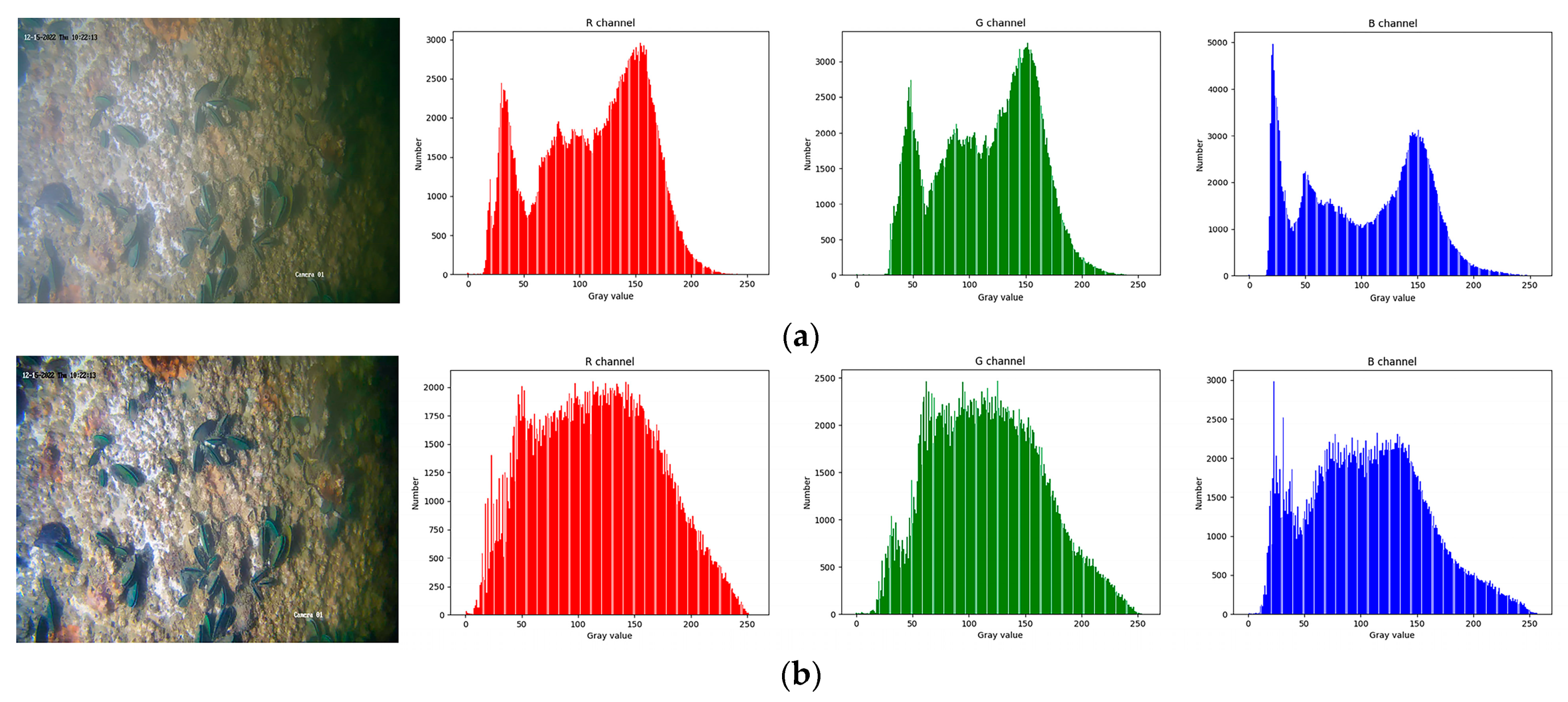
In this paper, the proposed method demonstrates excellent performance on an experimental dataset collected from the “Offshore Oil Platform HYSY-163” situated in the Beibu Gulf area of China. Figure 1 illustrates the results of the original image and the processed image using the three color channels (R, G, and B). The reconstructed image exhibits a more uniform distribution in the histogram and possesses enhanced clarity.
The remaining sections of the paper are organized as follows. Section 2 presents the details of our proposed method for underwater image enhancement tasks. In Section 3, we present the experimental results that demonstrate the effectiveness of our approach. Finally, Section 4 provides the concluding remarks.

2. Materials and Methods

In 2015, Makhzani et al. [
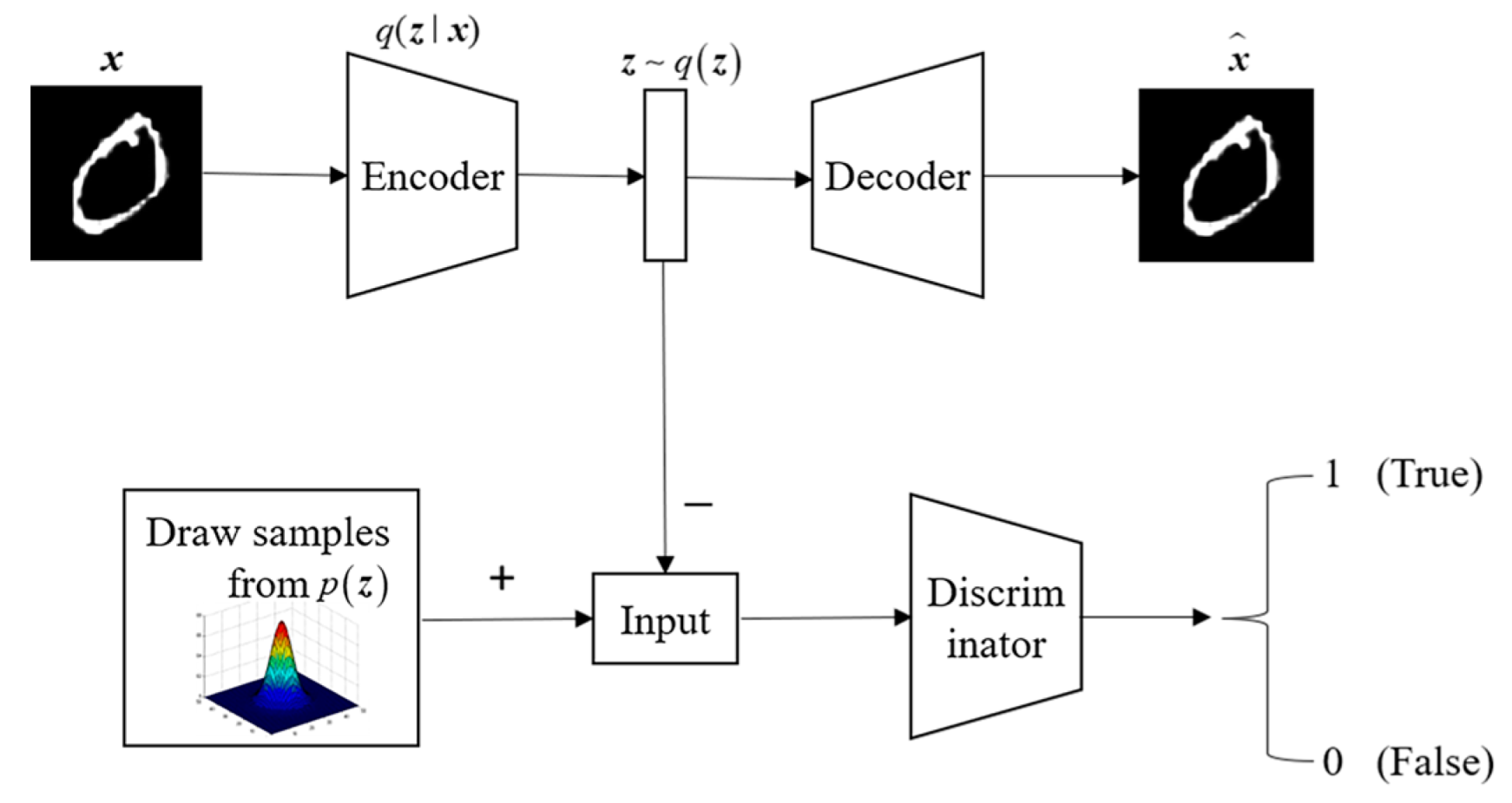
18] introduced the concept of adversarial autoencoder, which combines the adversarial generative network with the autoencoder network. The specific architecture of the proposed model is depicted in Figure 2. The adversarial autoencoder (AAE) model comprises two components: an autoencoder (AE) and a generative adversarial network (GAN). Adversarial training is incorporated into the autoencoder, enabling the dimensionally reduced data to adhere to a specific distribution. The training process of the adversarial autoencoder consists of two main parts. Firstly, it involves matching an aggregated posterior q z with an arbitrary prior distribution p ( z ) . To achieve this, an adversarial network is connected to the hidden code vector of the autoencoder. This adversarial network guides q z to align with p ( z ) , ensuring that the generated samples adhere to the desired prior distribution.
q z = x q z x p x d x
In the provided equation, p ( x ) represents the distribution of the target data from the training set.
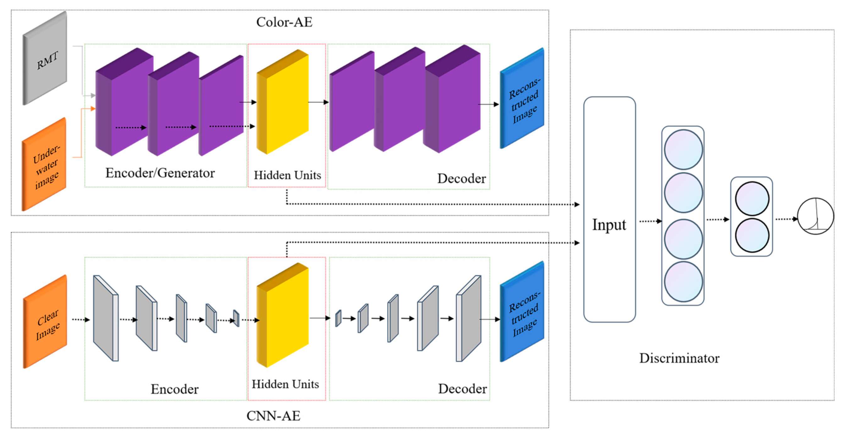
In this paper, we present an underwater image enhancement method named UW-AAE, which is based on the AAE model network. The overall framework diagram is illustrated in Figure 3. The model comprises two main modules: the autoencoder and the adversarial network. The autoencoder consists of the Color-AAE network and the pre-training model [19] CNN-AE. The discriminator plays a crucial role in guiding the hidden space of the Color-AAE network to progressively approach the hidden space of the pre-training model CNN-AE. It achieves this by accepting positive samples from the pre-training model and negative samples generated by the Color-AAE network.

2.1. Autoencoder Module

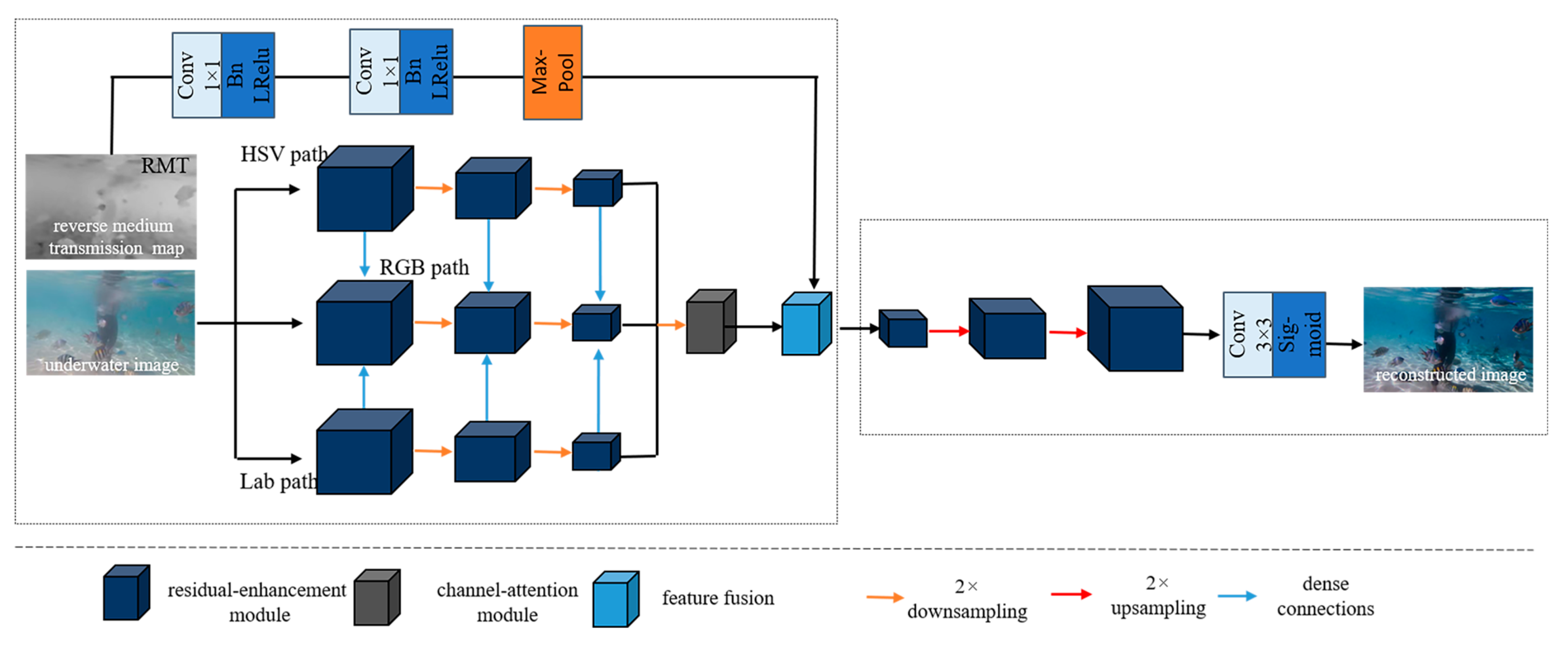
The structure of Color-AE is depicted in Figure 4, comprising two modules: the multi-color encoder and decoder. The multi-color encoder extracts features from both the underwater image and its reverse medium transmittance map. These features are then fused through the feature fusion module. The fused features are directed to the decoder network, which generates the reconstructed output. The underwater image undergoes a color space transformation, leading to the formation of three encoding paths: the HSV path, the RGB path, and the Lab path. In each path, the color space features undergo enhancement through three consecutive residual enhancement modules, resulting in three levels of feature representations. Additionally, a 2× downsampling operation is employed during this process. Furthermore, the features of the RGB path are combined with the corresponding features of the HSV path and the Lab path through dense connections to enhance the RGB path. Subsequently, the same level features of these three parallel paths are combined to form three sets of multicolor space encoder features. These three sets of features are then provided to their respective attention mechanism modules, which effectively capture rich and discriminative image features from multiple color spaces.
As the Reverse Medium Transmission (RMT) map can partially reflect the physical principles of underwater imaging [20], regions with higher pixel values in the RMT map correspond to more severe degradation in the corresponding underwater image regions. Consequently, the network assigns a larger weight response to the degraded regions of the image, acknowledging their significance in the enhancement process. The refinement of the RMT map is achieved through 1 × 1 convolutional layers with a step size of 2. Each convolutional layer is linked to the batch normalization layer and the Leaky ReLU activation function. Subsequently, a maximum pooling downsampling layer is employed to eliminate redundant repetitive information. The output of the feature fusion module is then transmitted to the corresponding residual enhancement module. Following three consecutive serial residual enhancement modules and two 2× upsampling operations, the decoder features are forwarded to the convolutional layers, leading to the reconstruction of the final result.

2.2. Residual Enhancement Module
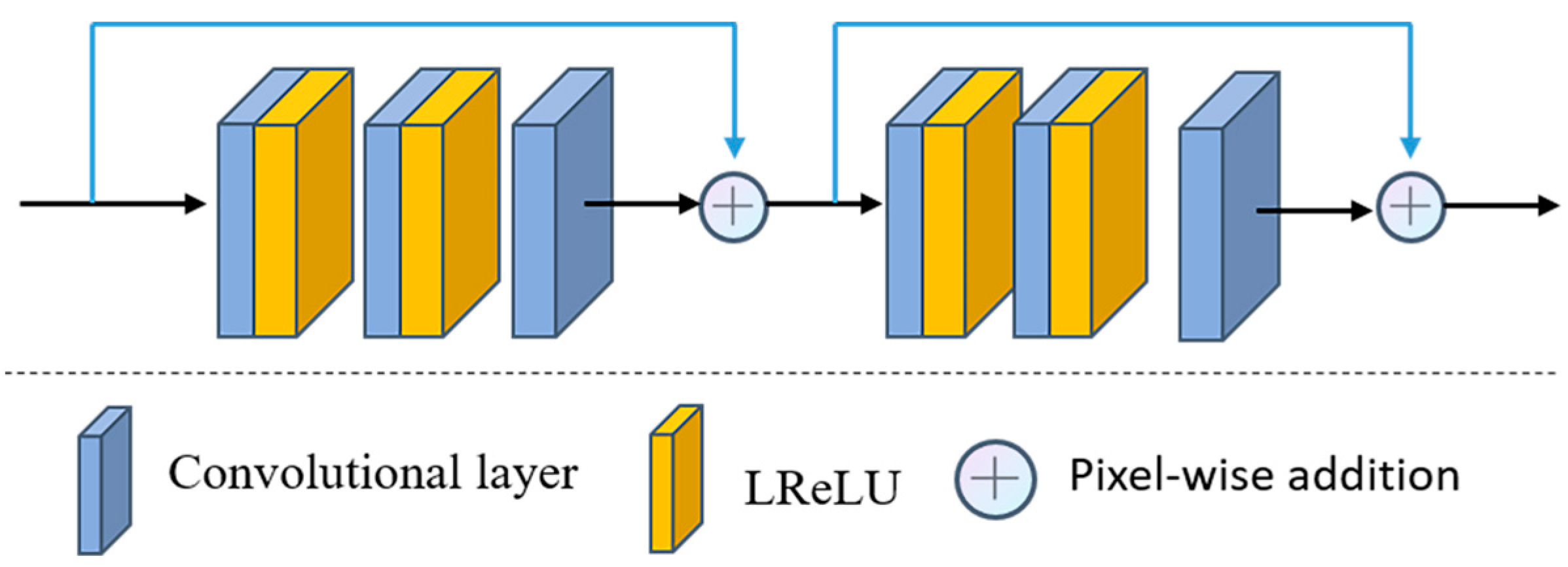
As depicted in Figure 5, each residual enhancement module comprises two residual blocks, each composed of three convolutions and two Leaky ReLU activation functions, with a 3 × 3 convolution kernel size and a step size of 1. Following each residual block, pixel-by-pixel addition is employed as a constant connection, with the purpose of enhancing the detailed features of the image and addressing the issue of gradient vanishing [21]. In each residual enhancement module, the convolutional layer maintains a consistent number of filters. Notably, the number of filters progressively increases from 128 to 512 in the encoder network, and conversely, it decreases from 512 to 128 in the decoder network.

2.3. Feature Attention Module

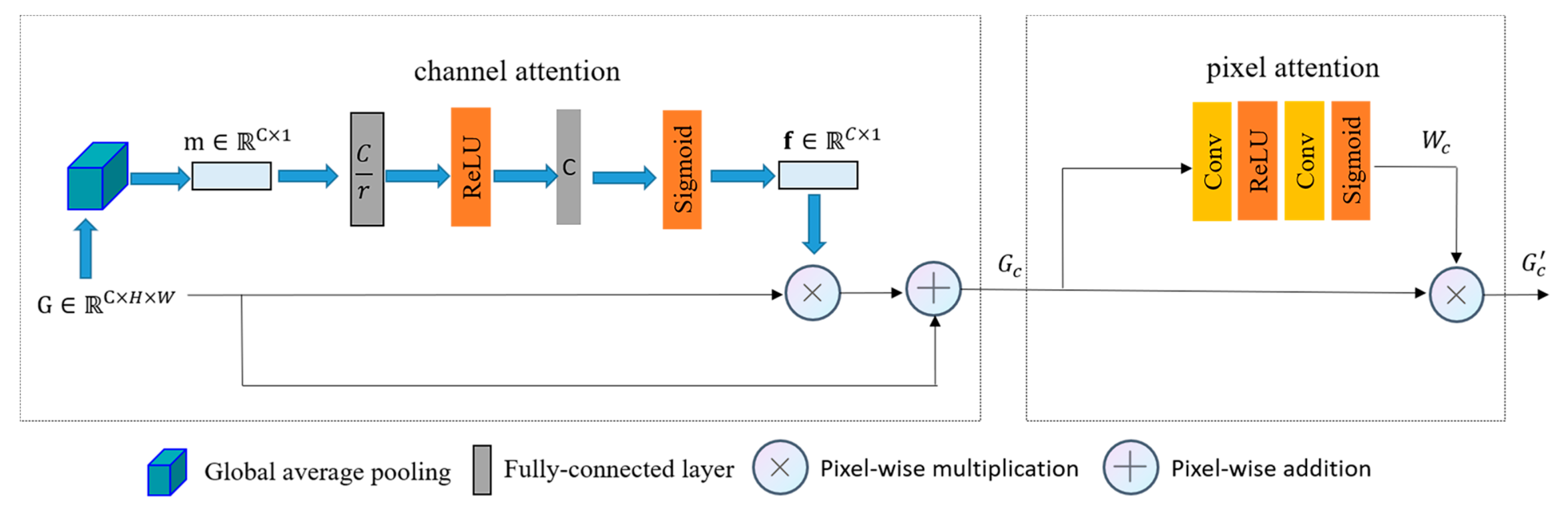
Considering the distinct characteristics of the three color space models—RGB, HSV, and Lab—these features, extracted from the three distinct color spaces, are expected to contribute differently. This study employs the channel attention mechanism and the pixel attention mechanism [22] to effectively handle the color variations in underwater images and account for the impact of different water qualities on the images. The specifics of the attention mechanism module are illustrated in Figure 6. Let G = Ser ( G 1 , G 2 , , G C ) R C × H × W represent the input feature, where G denotes the nominal mapping of a certain path, C is the number of channels of the feature mapping, Ser denotes the feature concatenation, and H and W are the height and width of the input image, respectively. In the channel attention mechanism, the spatial dimension of the input feature G is initially compressed. The feature maps of each channel are then downscaled through a global average pooling operation. This operation transforms the comprehensive spatial information along the channel dimension into a channel descriptor denoted as m R C × 1 , effectively minimizing the network’s parameter complexity. The central function of the channel descriptor is to produce an embedded global distribution of channel features, symbolizing the holistic significance of features within the channel. The mathematical expression for the k th term of m is as follows:
m k = 1 H × W i H j W F k i , j
where k [ 1 , C ] . m k represents the compressed “squeeze” representation of the channel, encapsulating the overarching perceptual information embedded within each channel. Moreover, F k denotes the weighting coefficients employed in the attention mechanism of the channel’s “excitation” representation, enabling the targeted amplification of distinct spatial positions within a particular channel. To fully capture individual channel dependencies, a self-gating mechanism [23] is employed to generate a set of modulation weights f R C × 1 .
f = σ W 2 δ W 1 z
In the equation, W 1 R   C r × C and W 2 R C × C r represent the weights of the two fully connected layers. σ denotes the Sigmoid activation function, δ represents the ReLU activation function, and denotes the convolution operation. The number of output channels for W 1 and W 2 is equal to C r and C , respectively. The hyper-parameter r defines the dimensionality relationship between the two fully connected layers, allowing control over the proportion of dimensionality reduction for the channel weights, thus influencing the model’s performance and computational efficiency. For computational purposes, r is set to 16; comprehensive details can be accessed in [23]. These weights are subsequently applied to the input features G to produce the output channel features G c . Moreover, to mitigate the issue of vanishing gradients and retain valuable information about the original features, we handle the channel attention weights in a similar mapping manner:
G c = G G s
where represents pixel-by-pixel addition, and denotes pixel-by-pixel multiplication.
The channel attention mechanism primarily concentrates on the allocation of weights across distinct channels. As a complementary technique to the channel attention mechanism, the pixel attention mechanism is centered on weight distribution across various pixel locations within a singular feature map, enabling the network to focus on regions with varying turbidity levels underwater. Illustrated in Figure 6, the pixel attention layer consists of two convolutional layers, each incorporating a ReLU activation function and a Sigmoid activation function:
W c = σ Conv δ C o n v G c G c
Con v represents the convolution operation, σ denotes the Sigmoid activation function, and δ denotes the ReLU activation function. A pixel-by-pixel multiplication of the input feature G c with the weights W c obtained from Equation (5) is performed:
G c = G c W c

2.4. Feature Fusion Module

Considering the need to perform underwater image enhancement with a focus on regions containing severe image degradation areas [24], we have designed a feature fusion module capable of adaptively selecting image features. This module processes both RGB image features and RMT image features by employing convolutional layers with different receptive fields. The selective utilization of these diverse features enhances the network’s ability to identify and address regions with significant image degradation, contributing to more effective underwater image enhancement. The RMT image serves as a representation of the physical laws governing underwater optical imaging. Higher pixel values within the RMT image indicate more severe degradation in the corresponding positions of the RGB image, necessitating a greater emphasis on the enhancement process. Leveraging the RMT image to guide the RGB image enhancement enables differentiation in the significance of various regions, thereby facilitating adaptive enhancement with varying degrees of emphasis. Training deep neural networks for RMT map estimation poses a challenge due to the unavailability of practical ground truth RMT maps for the input underwater images. To address this issue, we adopt the commonly used underwater image restoration algorithms’ image imaging model [25], which represents the quality-degraded image as follows:
I c x = J c x T x A c x 1 T x
Let x represent the coordinate of any pixel in the color image, where c ( R , G , B ) refers to the three color channels R, G, and B, respectively. I c corresponds to the image captured directly underwater, while J c denotes the ideally clear image. A c represents the ambient background light intensity in the R, G, and B channels. T ( x ) represents the medium transmittance of each pixel point, which signifies the percentage of radiation that arrives at the camera after reflection in the medium, relative to the scene radiation. This value indicates the degree of quality degradation in different regions.
Drawing inspiration from the dark channel prior [9], the DCP (Dark Channel Prior) method seeks the minimum value in the RGB channel for each pixel x within the local region Ω ( x ) centered at x . In other words, we have J DCP RGB ( x ) = m i n y Ω ( x ) m i n c ( R , G , B ) J c ( y ) . For an unfogged image of an outdoor ground surface, J DCP RGB ( x ) typically approaches zero because, in the local facets (represented by units of Ω ( x ) ), at least one of the three color channels generally contains a low-intensity pixel. In the context of Equation (7), the term involving J c is rounded off due to its proximity to zero, and this enables the estimation of the medium transmittance, denoted as follows:
T ~ RGB x = 1 m i n y Ω x m i n c R , G , B I c y A c
Additionally, it can be expressed as follows:
T ~ RGB x = m a x c , y Ω x 1 I c y A c = m a x c , y Ω x A c I c y A c
According to the Beer–Lambert law of light attenuation, the transmittance is commonly expressed as an exponential decay term.
T ~ x = e β d x
where d 0 is the distance from the camera to the radiating object, and β is the spectral volume attenuation coefficient, ensuring that T ~ 0 . In cases where Equation (10) results in a negative number (i.e., A c < I c ( y ) , y Ω ( x ) ), the value of T ~ becomes negative, making the use of Equation (8) inaccurate. To address this issue, an estimation algorithm [26] based on prior information is employed to obtain the influence of the medium transmittance map. In this paper, the medium transmittance is estimated as follows:
T ~ x = m a x c , y Ω x A c I c y m a x A c , 1 A c
The estimated medium transmittance map, denoted as T ~ , represents a local region of size 15 × 15 centered on Ω ( x ) . Here, c denotes the color channel, and the medium transmittance estimate is related to the uniform background light A c .
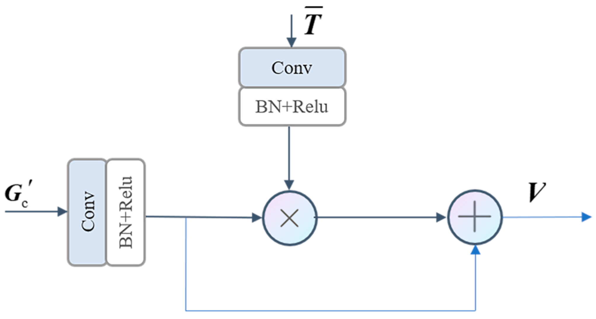
The schematic diagram of the proposed feature fusion module is illustrated in Figure 7, where G c R C × H × W and V R C × H × W represent the input features and output features in the feature fusion module, respectively. The RMT map T ¯ x = 1   -   T ~ ( x ) , with T ¯ R H × W , represents the reverse medium transmittance map in the range of [0, 1]. This map acts as a feature selector, assigning weights to different spatial locations of the features based on their respective importance. High-quality degraded pixels, represented by larger RMT values, are assigned higher weights. To extract RMT features and obtain rich local area features, a dilated convolution with a dilation rate of 2, a convolution kernel size of 3 × 3, and a convolution step of 1 are employed. Additionally, a convolution with a convolution kernel size of 3 × 3, a padding of 1, and a step size of 2 is used to extract RGB image features. The RMT features act as auxiliary information for feature selection of RGB image features, allowing the network to adaptively select regional features with severe image degradation.

2.5. Loss Function

The loss function of the proposed UW-AAE model in this study comprises two main components: the Color-AE module L f and the adversarial network module L GAN . L f is a linearly optimized combination of the reconstruction loss function L 1 and the perceptual loss function L VGG , utilized to train the Color-AE module. The final loss L f is expressed as follows:
L f = L 1 + λ L VGG
The hyperparameter λ is used as a trade-off factor to balance the weights of the loss functions L 1 and L VGG . In this study, λ is set to 0.05. L 1 represents the difference between the reconstructed result K ^ and the corresponding true data K , and can be expressed as follows:
L 1 = m = 1 H n = 1 W K ^ ( m , n ) K ( m , n ) 2
To enhance the visual quality of the image, the VGG19 pre-training model [27] is incorporated into the framework. The perceptual loss, denoted as L VGG , is computed based on the disparity between the reconstructed image response from the convolutional neural network and the feature mapping of the target image. Here, ϕ k represents the high-level feature extracted from the k th convolutional layer. The distance between the reconstructed result K ^ and the feature representation of the ground truth image K is defined as follows:
L V G G = m = 1 H n = 1 W ϕ k ( K ^ ) ( m , n ) ϕ k ( K ) ( m , n )
This formula delineates the establishment of a perceptual loss at each pixel position ( m , n ) through the computation of the absolute disparity between the feature representations of the reconstructed image and the truth image at feature layer k . This perceptual loss is computed as the disparity between the reconstructed image and the truth image. This metric of disparity serves to gauge the semblance between the reconstructed image and the truth image within the feature space. This methodology offers the advantage of proficiently steering the optimization of the reconstructed image, circumventing the necessity for real data, which can be arduous to acquire.
The generator G in the adversarial network serves as the encoder of Color-AE, generating negative samples denoted as z _ . In other words, z _ = En ( x ) . The discriminator receives both the positive samples z + from the encoder of the pre-trained CNN-AE and the negative samples z _ . The loss function of the discriminator in the adversarial network is given as follows:
L GAN = m i n G m a x D E z + ~ p z + l o g D z + + E x ~ P data l o g 1 D E n x
where p z + represents the hidden space distribution of the pre-trained model CNN-AE, and P data is the training data distribution. Through adversarial training, p z + is enforced to approach the hidden space of Color-AEE.

3. Experimentation and Analysis

3.1. Experimental Environment and Parameter Design

To validate the effectiveness of the algorithm, this experiment was implemented on the Pycharm simulation platform, and the network was trained using the PyTorch deep learning framework. The UW-AAE model was executed on a computer equipped with an Intel(R) Core(TM) i5-7300HQ CPU @ 2.50 GHz and a GTX 1080 Ti GPU. The network training process took approximately 42 h, while the testing time was approximately 6 min. Random rotation and horizontal flipping were employed for data augmentation during UW-AAE training. Additionally, all input images in the training set were resized to 256 × 256 pixels. The model parameter batch was set to 16, the learning rate to 0.0002, and the hidden vector dimension to 128. To determine an appropriate value for the number of epochs, Figure 8 illustrates the evolution of validation loss and training loss functions during the training process of the method proposed in this study. As the number of epochs increases, the loss function values exhibit a consistent decline. Around epoch 120, the loss value shows a tendency to stabilize, indicating the onset of convergence of the loss function. This observation suggests that our method demonstrates a favorable fitting performance. During adversarial training, the generator and discriminator are trained alternately. The discriminator is trained once, and the generator is updated twice in each iteration. Both the generator and discriminator use the Adam optimizer, with β 1 set to 0.5 and β 2 set to 0.999. The adversarial learning rate ( l r ) is set to 0.0002. To mitigate overfitting during the training process, a dropout technique is applied to the autoencoder (with a dropout ratio of 0.3).
The training set used in this experiment consists of 5200 real underwater images and their corresponding clear images, which were obtained from Underwater-ImageNet [28]. Due to the varying attenuation of different wavelengths of light in seawater, real underwater images often exhibit blue-green color tones. Similarly, the dataset provided by Underwater-ImageNet also exhibits these blue-green attenuation characteristics. The test set is divided into two subsets: test set A, containing 60 real underwater images without reference, and test set B, containing 45 underwater images with reference images for evaluation.

3.2. Subjective Evaluation

The enhanced results of the UW-AAE model that we proposed are compared with six existing traditional algorithms and deep learning-based underwater image enhancement methods, namely UDCP [10], HE [29], Fusion-based [27], ULAP [12], Ucolor [15], and FunieGAN [27], respectively. Representative images with greenish, bluish tints, as well as cloudy and dark lighting conditions are selected for analyzing the contrast and color restoration performances of each algorithm from a subjective visual perspective. Figure 9 and Figure 10 present a comparison of the aforementioned algorithms on the unreferenced underwater image test set A and the fully referenced underwater image test set B, respectively. While the UDCP algorithm exhibits a favorable performance in handling more turbid images, it tends to reduce the brightness of the image and is less effective in restoring images with greenish and bluish tones. The HE algorithm exhibits some ability to restore color in different types of images, but it tends to produce oversaturation. On the other hand, Ucolor enhances the contrast and brightness of the image but falls short in effectively removing turbidity. FunieGAN and ULAP do not perform well in recovering the original color of heavily bluish-greenish images, and in low-light situations, they introduce other colors. The Fusion-based method effectively recovers the color distortion of the image, but it may occasionally suffer from color deviation. In contrast, the algorithm we proposed in this study successfully enhances the image’s brightness and contrast while preserving the structural information and accurately recovering the color of degraded underwater images.

3.3. Analysis of Objective Indicators

3.3.1. Objective Metrics Analysis on Test Set A

To further validate the effectiveness of our proposed method, two non-reference image evaluation metrics, namely Natural Image Quality Evaluator [30] (NIQE) and Underwater Color Image Quality Evaluation [31] (UCIQE), were used to objectively analyze and compare the enhancement effects of the aforementioned seven algorithms on the images from test set A.
NIQE is a non-reference image quality evaluation metric based on Multivariate Gaussian (MVG) modeling. It involves obtaining a collection of features from the original image using a highly regular Natural Scene Statistic (NSS) model. These features are then fitted to an MVG model. In the underwater image evaluation process, the quality of the image being evaluated is expressed as the distance between the multivariate Gaussian fitting parameters of the NSS features extracted from the image and the parameters of the image model being evaluated. A lower value of NIQE indicates higher quality of the enhanced image. It is computed as follows:
D v 1 , v 2 , Σ 1 , Σ 2 = v 1 v 2 T Σ 1 + Σ 2 2 1 v 1 v 2
where v 1 , v 2 , Σ 1 , and Σ 2 represent the mean vector and covariance matrix of the natural MVG model and the distorted image MVG model, respectively.
The underwater color image quality evaluation metric UCIQE, used for images in the CIELab space, is a linear combination of underwater image color concentration, saturation, and contrast. It is designed to quantitatively assess the non-uniform color bias, blurriness, and low contrast of an image, and is defined as follows:
UCIQE = c 1 × σ c + c 2 × μ s + c 3 × c o n l
where σ c represents the standard deviation of chromaticity, c o n l denotes the contrast of luminance, and μ s is the average value of saturation. The parameters c 1 , c 2 , and c 3 are the weighting coefficients, which are set to 0.4860, 0.2576, and 0.2745, respectively. A higher value of UCIQE indicates that the image contains more details, and a more desirable enhancement effect has been achieved.
As observed in Table 1, our method demonstrates a substantial improvement in the reconstructed images, with an average reduction of 27.8% in the NIQE value compared to the unprocessed real underwater images. The average NIQE value is lower than that of the other six algorithms. Lower NIQE values correspond to higher image quality, which suggests that the reconstructed image quality is the most desirable among all the evaluated effects. As depicted in Table 2, our method shows a notable improvement in the processed images, with an average increase of more than 28.8% in the UCIQE value compared to the unprocessed real underwater images. This increase indicates a significant enhancement in color concentration, saturation, and contrast, suggesting that the images have been significantly improved in these aspects. However, it is worth noting that the average score is lower than that of some traditional algorithms, and the excessively high UCIQE scores may result from the image exhibiting phenomena of oversaturation and unnatural effects, such as those produced by the HE algorithm. In summary, our method demonstrates strong performance in visualization and achieves superior enhancement of underwater images.

3.3.2. Analysis of Objective Metrics on Test Set B

To quantitatively evaluate the performance of different algorithms on test set B, two full-reference evaluation metrics, namely Structural Similarity (SSIM) and Peak Signal-to-Noise Ratio (PSNR), are employed. SSIM assesses the similarity between the enhanced image and the reference image in terms of structure, contrast, and brightness. A higher SSIM score indicates that the enhanced result bears greater similarity to the true image as a whole. On the other hand, PSNR measures the level of distortion in the enhanced image with respect to the reference image. A higher PSNR score suggests that the enhanced image has undergone less distortion in comparison to the true value image. Table 3 and Table 4 present the scores of the different algorithms based on SSIM and PSNR metrics. When compared to both the input underwater image and the other six algorithms, our method has attained optimal scores. These results indicate that the enhanced image exhibits minimal distortion and preserves image content and structural information closely resembling the reference image.

3.4. Ablation Studies

To assess the effectiveness of the proposed UW-AAE network and its key module, the attention mechanism, ablation experiments were conducted. Figure 11 illustrates the comparison between the results obtained with the canny operator [32] processing the original image, without the inclusion of the attention module, and the results obtained using this paper’s algorithm after enhancement. It is evident that the regions with significant visual quality improvement are marked in red on the matrix.
As depicted in Figure 11, when compared with the original unprocessed image, the colors of the image have been noticeably corrected, leading to an improvement in overall image clarity. Additionally, the results obtained through the proposed method exhibit enhanced edge detection capabilities, indicating that the image retains more content information and possesses a superior ability to enhance image details.
SSIM and PSNR were selected as the objective evaluation indices for the ablation experiments, and the corresponding results are presented in Table 5. It is evident from the table that the algorithm proposed by us, equipped with the attention mechanism module, achieves the most favorable results among all the variations.

3.5. Running Time

We recorded the time consumed by various algorithms to process images of size 640 × 480 and listed the results in Table 6. It is observed that the HE algorithm exhibits the fastest processing speed, while our algorithm is not the fastest. This disparity can be attributed to the more complex structure of the proposed algorithm, which yields favorable results when confronted with diverse water quality scenarios.

4. Conclusions

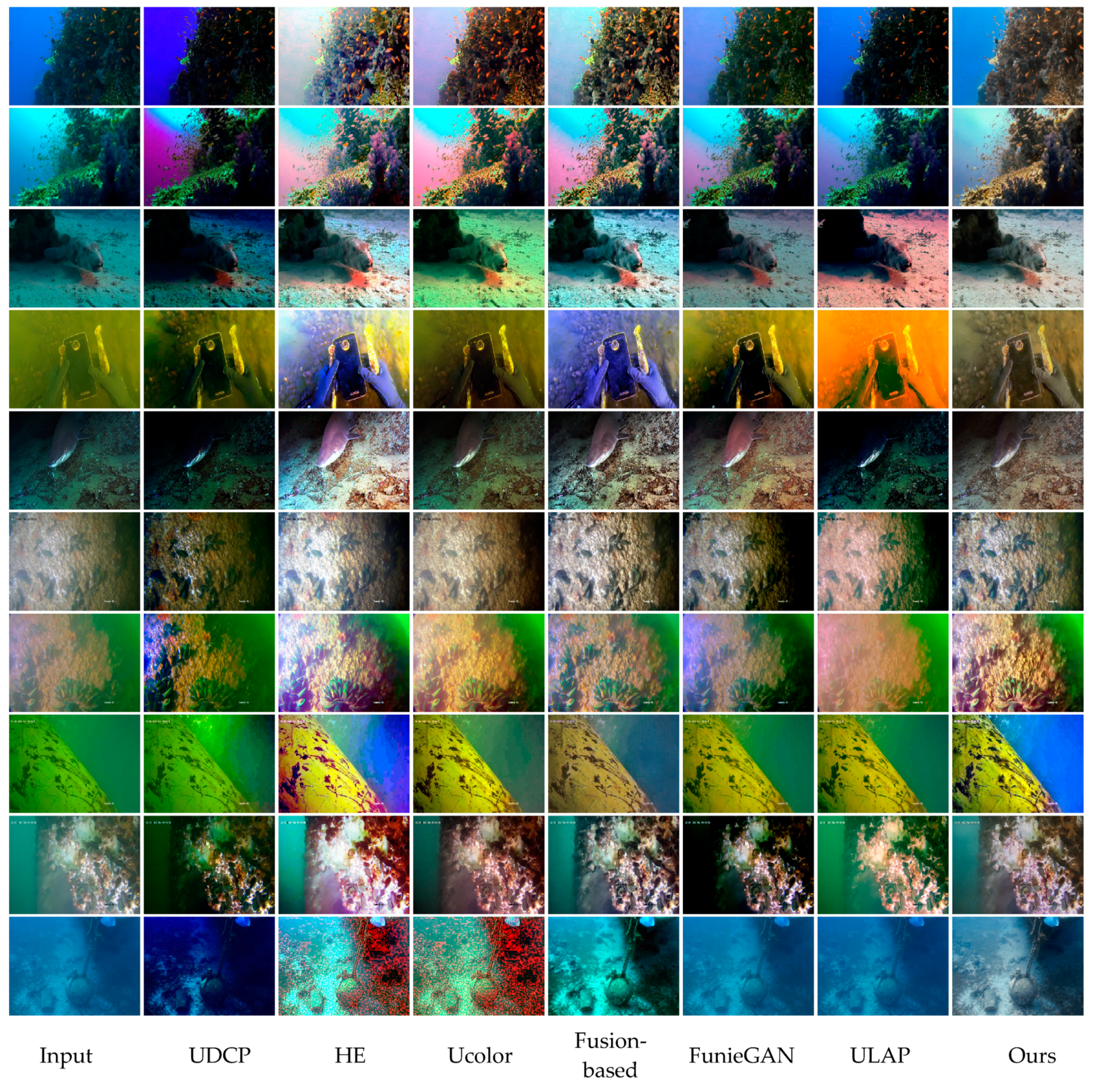
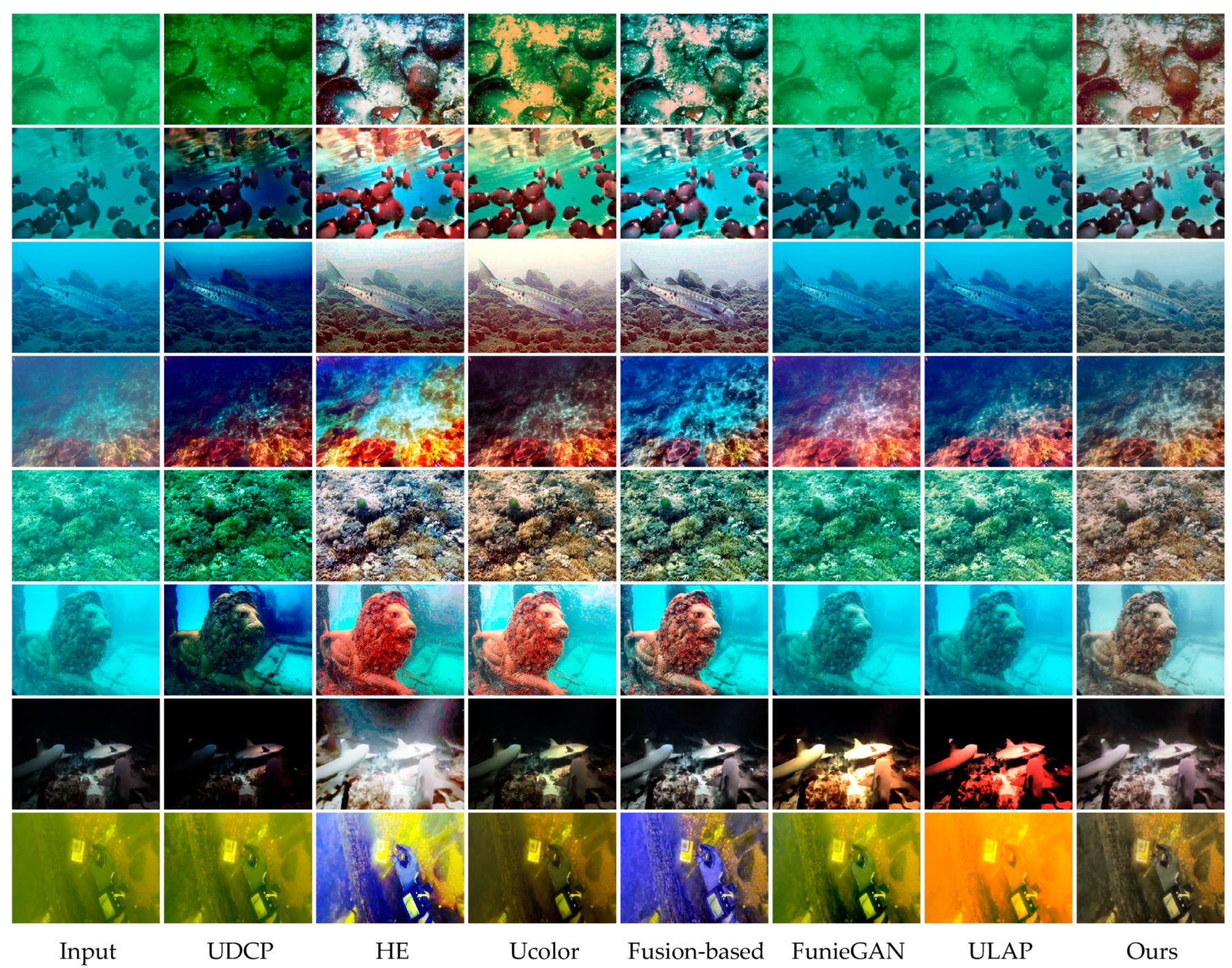
In this paper, to address the challenges of color deviation and low contrast in underwater images, we present an underwater image enhancement method based on the attention mechanism and adversarial autoencoder. By incorporating positive samples from the pre-trained model and negative samples generated by the encoder, the discriminator guides the autoencoder’s hidden space to approximate that of the pre-trained model. Furthermore, the encoder features, extracted using the attention mechanism, are fused with the features from the reverse medium transmittance map in the feature fusion module. This enhances the network’s ability to respond to regions with degraded image quality. The comparison experiments demonstrate that the reconstructed images outperform the existing six algorithms. When compared with the unprocessed real underwater images, the average Natural Image Quality Evaluator value is reduced by 27.8%, the average Underwater Color Image Quality Evaluation value is improved by 28.8%, and the average Structural Similarity and Peak Signal-to-Noise Ratio values are enhanced by 35.7% and 42.8%, respectively. The method exhibits excellent visual effects, effectively restoring the real scene of underwater images and enhancing the visibility of underwater target objects. It holds the potential to be utilized by underwater robots in future applications such as exploring marine resources and cleaning the bottoms of large ships.
Our proposed method is not without limitations. Primarily, our approach emphasizes underwater image color correction and contrast enhancement, but it may fall short in addressing the enhancement challenges posed by extremely turbid underwater images. To address this limitation, future research endeavors could focus on expanding the dataset to enhance the accuracy of transmission map estimation and bolster the model’s overall robustness. In the future, we will continue to explore the combination of traditional methods with deep learning-based approaches to develop more innovative interaction designs. Moreover, we aim to generalize our algorithms to various other domains.

Author Contributions

Conceptualization, G.L. and G.H.; methodology, G.L. and G.H.; software, G.H.; validation, G.L.; formal analysis, Z.J.; investigation, G.H. and C.L.; resources, Z.J. and G.L.; data curation, G.H.; writing—original draft preparation, G.H.; writing—review and editing, Z.J. and G.L.; visualization, G.H.; supervision, G.L.; project administration, G.L.; funding acquisition, Z.J. and G.L. All authors have read and agreed to the published version of the manuscript.

Funding

This research was funded by National Key Research and Development Program of China, grant number 2022YFD2401100 and Shanghai Municipal Science and Technology Commission Innovation Action Plan, grant number 20dz1206500.

Institutional Review Board Statement

Not applicable.

Informed Consent Statement

Not applicable.

Data Availability Statement

Our experiment was conducted on the Underwater-ImageNet Dataset [28].

Acknowledgments

I would like to express my heartfelt gratitude to the Shanghai Engineering Research Center of Hadal Science and Technology for their technical expertise and generous financial support. I am also deeply appreciative of the platform provided by China National Offshore Oil Corporation (CNOOC). Your contributions have been instrumental in the success of this endeavor. Thank you for your invaluable assistance and support.

Conflicts of Interest

The authors declare no conflict of interest.

References

  1. Chen, G.J.; Chen, W.; Wang, Z.M.; Guo, T.Z.; Xia, X.M.; Xu, L.J. Design and Dynamic Performance Research of Underwater Inspection Robots. Wirel. Commun. Mob. Comput. 2022, 2022, 3715514. [Google Scholar] [CrossRef]
  2. Nardelli, B.B.; Cavaliere, D.; Charles, E.; Ciani, D. Super-Resolving Ocean Dynamics from Space with Computer Vision Algorithms. Remote Sens. 2022, 14, 1159. [Google Scholar] [CrossRef]
  3. Gaudron, J.O.; Surre, F.; Sun, T.; Grattan, K.T.V. Long Period Grating-based optical fibre sensor for the underwater detection of acoustic waves. Sens. Actuator A-Phys. 2013, 201, 289–293. [Google Scholar] [CrossRef]
  4. Yan, Z.; Ma, J.; Tian, J.W.; Liu, H.; Yu, J.G.; Zhang, Y. A Gravity Gradient Differential Ratio Method for Underwater Object Detection. IEEE Geosci. Remote Sens. Lett. 2014, 11, 833–837. [Google Scholar] [CrossRef]
  5. Raveendran, S.; Patil, M.D.; Birajdar, G.K. Underwater image enhancement: A comprehensive review, recent trends, challenges and applications. Artif. Intell. Rev. 2021, 54, 5413–5467. [Google Scholar] [CrossRef]
  6. Zhuang, P.X.; Li, C.Y.; Wu, J.M. Bayesian retinex underwater image enhancement. Eng. Appl. Artif. Intell. 2021, 101, 104171. [Google Scholar] [CrossRef]
  7. Iqbal, K.; Odetayo, M.; James, A.; Salam, R.A.; Talib, A.Z.H. Enhancing the Low Quality Images Using Unsupervised Colour Correction Method. In Proceedings of the IEEE International Conference on Systems, Man and Cybernetics, Istanbul, Turkey, 10–13 October 2010. [Google Scholar]
  8. Zhou, J.C.; Zhang, D.H.; Zhang, W.S. Classical and state-of-the-art approaches for underwater image defogging: A comprehensive survey. Front. Inform. Technol. Electron. Eng. 2020, 21, 1745–1769. [Google Scholar] [CrossRef]
  9. He, K.M.; Sun, J.A.; Tang, X.O. Single Image Haze Removal Using Dark Channel Prior. In Proceedings of the IEEE-Computer-Society Conference on Computer Vision and Pattern Recognition Workshops, Miami Beach, FL, USA, 20–25 June 2009; pp. 2341–2353. [Google Scholar]
  10. Drews, P.; do Nascimento, E.; Moraes, F.; Botelho, S.; Campos, M. Transmission Estimation in Underwater Single Images. In Proceedings of the IEEE International Conference on Computer Vision (ICCV), Sydney, Australia, 1–8 December 2013; pp. 825–830. [Google Scholar]
  11. Peng, Y.T.; Cosman, P.C. Underwater Image Restoration Based on Image Blurriness and Light. IEEE Trans. Image Process. 2017, 26, 1579–1594. [Google Scholar] [CrossRef]
  12. Song, W.; Wang, Y.; Huang, D.M.; Tjondronegoro, D. A Rapid Scene Depth Estimation Model Based on Underwater Light Attenuation Prior for Underwater Image Restoration. In Proceedings of the 19th Pacific-Rim Conference on Multimedia (PCM), Hefei, China, 21–22 September 2018; pp. 678–688. [Google Scholar]
  13. Li, C.Y.; Anwar, S.; Porikli, F. Underwater scene prior inspired deep underwater image and video enhancement. Pattern Recognit. 2020, 98, 107038. [Google Scholar] [CrossRef]
  14. Wang, Y.D.; Guo, J.C.; Gao, H.; Yue, H.H. UIEC”2-Net: CNN-based underwater image enhancement using two color space. Signal Process.-Image Commun. 2021, 96, 116250. [Google Scholar] [CrossRef]
  15. Li, C.Y.; Anwar, S.; Hou, J.H.; Cong, R.M.; Guo, C.L.; Ren, W.Q. Underwater Image Enhancement via Medium Transmission-Guided Multi-Color Space Embedding. IEEE Trans. Image Process. 2021, 30, 4985–5000. [Google Scholar] [CrossRef]
  16. Li, J.; Skinner, K.A.; Eustice, R.M.; Johnson-Roberson, M. WaterGAN: Unsupervised Generative Network to Enable Real-Time Color Correction of Monocular Underwater Images. IEEE Robot. Autom. Lett. 2018, 3, 387–394. [Google Scholar] [CrossRef]
  17. Goodfellow, I.; Pouget-Abadie, J.; Mirza, M.; Xu, B.; Warde-Farley, D.; Ozair, S.; Courville, A.; Bengio, Y. Generative Adversarial Networks. Commun. ACM 2020, 63, 139–144. [Google Scholar] [CrossRef]
  18. Makhzani, A.; Shlens, J.; Jaitly, N.; Goodfellow, I.; Frey, B. Adversarial Autoencoders. arXiv 2016, arXiv:1511.05644. [Google Scholar]
  19. Hashisho, Y.; Albadawi, M.; Krause, T.; von Lukas, U.F. Underwater Color Restoration Using U-Net Denoising Autoencoder. In Proceedings of the 11th International Symposium on Image and Signal Processing and Analysis (ISPA), Dubrovnik, Croatia, 23–25 September 2019; pp. 117–122. [Google Scholar]
  20. Yan, K.; Liang, L.Y.; Zheng, Z.Q.; Wang, G.Q.; Yang, Y. Medium Transmission Map Matters for Learning to Restore Real-World Underwater Images. Appl. Sci. 2022, 12, 5420. [Google Scholar] [CrossRef]
  21. He, K.M.; Zhang, X.Y.; Ren, S.Q.; Sun, J. Deep Residual Learning for Image Recognition. In Proceedings of the 2016 IEEE Conference on Computer Vision and Pattern Recognition (CVPR), Seattle, WA, USA, 27–30 June 2016; pp. 770–778. [Google Scholar]
  22. Sun, W.Y.; Liu, B.D. ESinGAN: Enhanced Single-Image GAN Using Pixel Attention Mechanism for Image Super-Resolution. In Proceedings of the 15th IEEE International Conference on Signal Processing (ICSP), Beijing, China, 6–9 December 2020; pp. 181–186. [Google Scholar]
  23. Hu, J.; Shen, L.; Sun, G. Squeeze-and-Excitation Networks. In Proceedings of the 31st IEEE/CVF Conference on Computer Vision and Pattern Recognition (CVPR), Salt Lake City, UT, USA, 18–23 June 2018; pp. 7132–7141. [Google Scholar]
  24. Chen, E.R.; Ye, T.; Chen, Q.R.; Huang, B.; Hu, Y.D. Enhancement of Underwater Images with Retinex Transmission Map and Adaptive Color Correction. Appl. Sci. 2023, 13, 1973. [Google Scholar] [CrossRef]
  25. Jaffe, J.S. Computer modeling and the design of optimal underwater imaging systems. IEEE J. Ocean. Eng. 1990, 15, 101–111. [Google Scholar] [CrossRef]
  26. Peng, Y.T.; Cao, K.M.; Cosman, P.C. Generalization of the Dark Channel Prior for Single Image Restoration. IEEE Trans. Image Process. 2018, 27, 2856–2868. [Google Scholar] [CrossRef]
  27. Islam, M.J.; Xia, Y.Y.; Sattar, J. Fast Underwater Image Enhancement for Improved Visual Perception. IEEE Robot. Autom. Lett. 2020, 5, 3227–3234. [Google Scholar] [CrossRef]
  28. Fabbri, C.; Islam, M.J.; Sattar, J. Enhancing Underwater Imagery using Generative Adversarial Networks. In Proceedings of the IEEE International Conference on Robotics and Automation (ICRA), Brisbane, Australia, 21–25 May 2018; pp. 7159–7165. [Google Scholar]
  29. Muniyappan, S.; Allirani, A.; Saraswathi, S. A Novel Approach for Image Enhancement by Using Contrast Limited Adaptive Histogram Equalization Method. In Proceedings of the 4th International Conference on Computing, Communications and Networking Technologies (ICCCNT), Tiruchengode, India, 4–6 July 2013. [Google Scholar]
  30. Mittal, A.; Soundararajan, R.; Bovik, A.C. Making a “Completely Blind” Image Quality Analyzer. IEEE Signal Process. Lett. 2013, 20, 209–212. [Google Scholar] [CrossRef]
  31. Yang, M.; Sowmya, A. An Underwater Color Image Quality Evaluation Metric. IEEE Trans. Image Process. 2015, 24, 6062–6071. [Google Scholar] [CrossRef] [PubMed]
  32. Canny, J. A computational approach to edge detection. IEEE Trans. Pattern Anal. Mach. Intell. 1986, 8, 679–698. [Google Scholar] [CrossRef] [PubMed]
Figure 1. Comparison of visual effects and histogram results of R, G, and B channels before and after image processing using our proposed method. (a) The original image and histogram of its R, G, and B channels. (b) The reconstructed image and histogram of its R, G, and B channels.
Applsci 13 09956 g001
Figure 2. The structural diagram of the adversarial autoencoder model.
Applsci 13 09956 g002
Figure 3. The overall framework of the underwater image enhancement method, UW-AAE, which is based on the improvement of the AAE model.
Applsci 13 09956 g003
Figure 4. The structure of Color-AE for multi-color spatial encoding.
Applsci 13 09956 g004
Figure 5. The residual enhancement network.
Applsci 13 09956 g005
Figure 6. Feature attention module.
Applsci 13 09956 g006
Figure 7. Feature fusion module.
Applsci 13 09956 g007
Figure 8. The variation of the loss function during the training process.
Applsci 13 09956 g008
Figure 9. Visual comparison of different types of images (from test set A) enhanced by six state-of-the-art algorithms with our proposed approach.
Applsci 13 09956 g009
Figure 10. Visual comparison of different types of images (from test set B) enhanced by six state-of-the-art algorithms with our proposed approach.
Applsci 13 09956 g010
Figure 11. Results of the ablation study. (a) Original image, (b) de-attentioning mechanism, (c) our proposed methodology.
Applsci 13 09956 g011
Table 1. Comparison of the NIQE evaluation index results on test set A. Bold indicates the minimum value of NIQE for each group, and lower NIQE values indicate higher image quality.
ImageInputUDCPHEUcolorFusionFunieGANULAPOurs
image17.1425.9853.9774.7743.9005.7846.5323.229
image25.1385.1493.6504.1394.2564.8444.8243.383
image33.7163.3443.0113.4862.9813.6823.9373.403
image47.3605.1724.8646.2004.3345.3255.3054.122
image54.6405.2953.3554.5083.3813.9346.4423.266
image63.4363.5713.3773.5073.3293.5103.3873.249
image74.7044.1253.8994.0923.9694.3164.5904.105
Image83.5763.4112.9563.1172.8833.3933.2943.100
Image93.7703.8223.2903.5743.2784.0463.5203.471
Image104.6044.1388.2818.8753.4964.3094.5653.386
average 4.8094.4014.0664.6273.5814.3144.6403.471
Table 2. Comparison of UCIQE evaluation index results on test set A. Bold indicates the maximum value of each group of UCIQE, and higher values of UCIQE indicate higher image quality.
ImageInputUDCPHEUcolorFusionFunieGANULAPOurs
image10.4760.4690.4910.5170.4690.4920.5380.543
image20.5130.6330.5340.5500.5410.5830.5660.466
image30.3410.4490.4600.4490.4360.3700.5370.580
image40.3550.4960.5260.4480.5650.5550.4860.427
image50.3380.4290.4760.3780.4430.4350.4550.443
image60.3510.4500.4500.4060.4300.4600.4620.483
image70.3270.5490.4920.4350.4450.5380.3500.582
Image80.3840.4560.5790.4730.5690.4500.4910.484
Image90.3570.5210.5060.4470.4760.5030.4830.494
Image100.3760.5650.5580.5570.5240.3850.3710.422
average 0.3820.5020.5070.4660.4900.4770.4740.492
Table 3. Comparison of SSIM evaluation index results on test set B. Bold indicates the maximum value of each group of SSIM, where a higher SSIM value indicates that the image is more similar to the true reference image.
ImageInputUDCPHEUcolorFusionFunieGANULAPOurs
image10.3430.4050.9180.7340.8010.3840.4420.929
image20.6390.4450.8100.8390.9830.6420.7570.806
image30.7160.6020.8140.8380.7800.7780.6790.937
image40.7730.6510.6180.7410.7780.8240.7410.860
image50.7510.7090.8570.8590.8400.7910.7960.872
image60.6450.5890.7130.7480.7390.7120.7120.938
image70.1760.0450.3490.1840.2560.1530.0690.364
Image80.8110.7210.5990.7780.6480.6930.6890.883
average 0.6070.5210.7100.7150.7280.6220.6110.824
Table 4. Comparison of PSNR evaluation index results on test set B. The values in bold indicate the maximum PSNR score in each group. A higher PSNR score indicates less distortion in the enhanced image compared to the reference image.
ImageInputUDCPHEUcolorFusionFunieGANULAPOurs
image116.12713.93224.21023.78924.33016.76417.94124.979
image216.68810.04821.72323.54936.61216.08317.65326.808
image317.38111.49428.29521.17121.58218.50615.90729.935
image418.38316.13815.34521.06521.84324.19124.05127.226
image518.12519.82823.99923.33425.08026.78123.67228.045
image619.76811.89520.54620.12619.96520.79519.82827.230
image78.9587.80313.5349.39910.58610.6469.18411.648
Image827.83026.48414.87519.19223.60122.52814.69228.765
average 17.90814.70320.31620.20322.95019.53717.86625.580
Table 5. Objective evaluation index results of ablation study.
MethodologiesSSIMPENR
Original Image0.34316.127
De-attentioning Mechanisms0.91023.774
Ours0.92924.979
Table 6. Average processing time per image of algorithms.
Arithmetict/sArithmetict/s
UDCP6.756FunieGAN15.960
HE0.024ULAP0.823
Ucolor3.986Fusion0.371
Ours2.786
Disclaimer/Publisher’s Note: The statements, opinions and data contained in all publications are solely those of the individual author(s) and contributor(s) and not of MDPI and/or the editor(s). MDPI and/or the editor(s) disclaim responsibility for any injury to people or property resulting from any ideas, methods, instructions or products referred to in the content.

