Multilabel Genre Prediction Using Deep-Learning Frameworks

Abstract

In this study, transfer learning has been used to overcome multilabel classification tasks. As a case study, movie genre classification by using posters has been chosen. Six state-of-the-art pretrained models, VGG16, ResNet, DenseNet, Inception, MobileNet, and ConvNeXt, have been employed for this experiment. The movie posters have been obtained from Internet Movie Database (IMDB). The dataset has been divided using an iterative stratification technique. A sequence of dense layers has been added on top of each model and these models have been trained and fine-tuned. All the results of the models compared considered accuracy, loss, Hamming loss, F1-score, precision, and AUC metrics. When the metrics used were evaluated, the most successful result regarding accuracy has been obtained from the modified DenseNet architecture at 90%. Also, the ConvNeXt, which is the newest model among all, performed quite satisfactorily, reaching over 90% accuracy. This study uses an iterative stratification method to split an unbalanced dataset which provides more reliable results than the classical splitting method which is the common method in the literature. Also, the feature extraction capabilities of the six pretrained models have been compared. The outcome of this study shows promising results regarding multilabel classification. As for future work, it is planned to enhance this study by using natural language processing and ensemble methods.

1. Introduction

In the world of film, movie posters have long served as a visual gateway into the captivating stories that await within. With their striking imagery and carefully curated designs, movie posters not only entice audiences but also provide valuable insights into the genre and theme of a film. Analyzing movie posters and accurately predicting their genres can be a challenging task, but with the advent of advanced machine-learning techniques, the multilabel classification of movie posters based on genre has become a fascinating area of research.

Multilabel classification refers to the task of assigning multiple labels or tags to an input instance. In the context of movie posters, this involves identifying and assigning appropriate genre labels to posters based on their visual characteristics. Genres such as action, romance, comedy, horror, sci-fi, and many more encompass the vast landscape of film, each with its own unique visual cues and tropes. The ability to automatically classify movie posters into multiple genres not only facilitates efficient cataloging and organization but also opens up avenues for personalized recommendations, genre-based marketing strategies, and enhanced user experiences in the realm of film.

Multilabel classification has a wide variety of challenges including but not limited to label imbalance, dependency between labels, and choosing the appropriate evaluation metrics. In multilabel classification, a task often comes with an imbalanced dataset where some labels are more frequent than others. This issue can cause bias in the training process of the model which becomes prone to predicting dominant labels. Also, labels in multilabel classification problems can also carry different dependency levels. Some labels can be highly dependent, and others can be mutually exclusive. Furthermore, evaluating the performance of a multilabel classification task is not as straightforward as in a multiclass or binary class classification task. The accuracy cannot fully provide the big picture of the performance of the model. It needs to be used with Hamming loss, precision, recall, F1-score, etc.

The challenges inherent in the multilabel classification of movie posters are manifold. Movie posters exhibit intricate designs, incorporating various visual elements such as color schemes, typography, lighting, composition, and character depictions. Furthermore, posters can incorporate multiple genres, as films often blend different genres to create compelling narratives and attract diverse audiences. Accurately capturing these nuances and mapping them to appropriate genre labels requires sophisticated machine-learning models capable of discerning intricate patterns and representations from the visual data.

Computer science brings solutions to many problems in a broad range of areas including but not limited to medicine [1], education [2], military [3], and history [4]. An increasing number of studies have been conducted day by day and the image classification task is one of most popular topics in these computer vision studies [5].

Genre prediction is one of the most appealing tasks in classification problems. The genre gives a general idea about the movie as well as having an important effect on the movie selection. Proper classification of the genre is an important task in terms of the service provided to viewers such as recommendation systems.

The use of transfer-learning methods, which can be defined as using previously trained convolutional neural network (CNN) models to overcome similar tasks, has become very popular and yielded very successful results in computer vision-based applications such as image classification [6]. Machine-learning technologies, especially CNNs, can be applied in many areas because they can discover the complex structures of data by themselves [7]. CNN-based algorithms can automatically learn to extract the necessary features by using a multilayer network hierarchy and it can be adapted to solve different but similar problems [8].

Movie genre prediction studies are made by using visual, auditory, and textual features [9]. Classification of posters with visual features according to their genres by a machine-learning algorithm is one of these studies [10]. Posters are important because they create a first impression of the movie content and genre. In addition, posters are visual data suitable for computer vision applications.

The scope of this paper includes the multilabel genre classification of movie poster images. It employs the usage of six modern pretrained deep-learning models and various performance evaluation metrics.

This paper proposes multilabel classification models to achieve determining the genre of the movie based on the poster image. The novel part of this study is using a ConvNeXt model in the context of a multilabel classification problem and comparing the performance with former models. One of the most challenging parts of this study is that the number of movies in each genre are in different ranges. For example, while there are 552 films in the sport genre, there are 14,585 films in the drama film genre. Another problem is that a movie can have more than one genre. In order to overcome the mentioned problems, pretrained CNN models (VGG16, ResNet50, InceptionV3, DenseNet, MobileNet, and ConvNeXt) have been employed by using transfer-learning methods and the results are compared. When the results have been evaluated, according to the accuracy, loss, Hamming loss, F1-score, precision, and AUC (area under the receiver operating characteristic curve) metrics, it can be seen that the most successful model belonged to the pretrained DenseNet architecture with an accuracy rate of 90%. The ConvNeXt model also achieved the minimum loss score among the pretrained models.

The remainder of this paper is structured as follows. Section 2 includes the literature of the problem and summarization table. The proposed architectures for the multilabel classification problem are presented in Section 3. Section 4 illustrates the results of this experiment and unveils the evaluation details of the models. Lastly, Section 5 makes a conclusion.

2. Related Work

In the literature, the genre classification studies use different data types such as text, sound, images from a variety of sources like posters, fragments, and summaries. In this section, these studies will be summarized from a broad perspective.

Huang et al. [11] used movie trailers to determine movie genres. The support vector machine classifier was fed the visual and auditory features derived by the self-adaptive harmony search algorithm, which is a metaheuristic optimization algorithm. The genre of each film was determined using a majority voting system. The models were evaluated using the Apple Movie Trailers website and the IMDB dataset, which contains seven genres. The proposed model obtained a 91.9% accuracy rate.

Using visual and auditory features, Ekenel et al. [12] determined the content-based genre classification of TV programs and YouTube videos. A support vector machine (SVM) model was trained. On this model, the one-to-all method was used for the feature and genre variants. The final result was determined by combining the classifier’s output. The information about color and texture was represented by six low-level visual features that were also used to detect high-level features. The YouTube dataset was used to validate the model, which achieved an accuracy rate of 87.3%.

In their study, Fu et al. [13] used movie posters and summaries to autonomously detect film genres. The posters collected from popular foreign film sites and the relevant summaries from the Movie Database (TDMB) were used and four genres were determined. Features such as color, edge, texture, and face detection were removed from movie posters. The vector space model was utilized to extract text features from summaries. Using these features, two distinct support vector machines were trained to produce a poster classifier and a text classifier. On the outputs of these classifiers, the testing phase based on the ‘OR’ operation was performed as a fusion operator. The proposed model achieved an accuracy rate of 88.05%.

Simoes et al. [14] introduced a novel approach, CNN-MoTion, that utilized a convolutional neural network (CNN) model for the purpose of predicting movie genres from their respective trailers. A new dataset, denoted as LMTD (Labeled Movie Trailer Data), was generated, comprising over 3500 trailers that were categorized into four distinct genres, as per the study’s parameters. The model’s success rate, as determined by the accuracy metric, was 73.75%. The model under consideration exhibited a superior performance by approximately 5% in contrast to other well-known movie trailer classification techniques such as Gist, CENTRIST, and w-CENTRIST.

Chu et al. [15] introduced a deep neural network model which used visual appearance and object information for multilabel genre classification. Within the scope of the study, posters were taken using the IMDB dataset and 23 different genres were determined. AlexNet, a pretrained CNN model, was modified to extract visual features, and the YOLO method was used to detect objects on posters. It was determined that YOLO was effective in measuring the contribution of object detection to genre classification success. The proposed method achieved an L1 norm vector accuracy of 18.73%.

Sung et al. [16] proposed a deep-learning approach to predict movie genres from movie posters. To determine the optimal model for this classification problem, the transfer-learning technique was applied to contemporary pretrained models such as ResNet-50, VGG-16, and DenseNet-169. The final layers of the pretrained architectures were modified based on the nature of the problem. The Kaggle dataset was utilized and seven genres were defined to test the model. The DenseNet-169 model was determined to be the most successful based on its F1-score of 0.77 percent and ROC-AUC of 0.67 percent.

Arevalo et al. [17] presented a multimodal model, namely Gated Multimodal Unit (GMU), which utilizes gated neural networks to predict the genre of a movie based on its plot and poster. The GMU neural network architecture incorporates an internal unit that is intended to identify a transitional representation based on various data types. Furthermore, a dataset known as Multimodal-IMDB (MM-IMDB) was curated to cater to multimodel systems, encompassing a total of 23 distinct genres. The feature extraction and classification stages for text data involved the utilization of n-gram, word2vec, and RNN models. On the other hand, for image data, a pretrained VGG-Net, a redesigned 5-layer CNN network, and multilayer perceptron (MLP) were employed. The word2vec and MLP algorithms yielded the highest level of success in text classification, achieving an F-score of 0.59%. The results of the image classification indicated that the pretrained models outperformed the models developed from scratch, with an F-score of 0.43%. The multimodal GMU network demonstrated the highest level of performance, as evidenced by its F-score of 0.63%.

Hoang [18], in his study, performed genre classification by using movie plot summaries and machine-learning methods. The study utilized the bag of words and word2vec techniques to extract features, and subsequently employed the Naive Bayes, XGBoost, and Gated Recurrent Unit (GRU) classifiers for classification purposes. The models were tested using the IMDB dataset, which comprises 20 distinct genres. The findings of the experiments indicated that the GRU neural networks exhibited the highest level of success, as evidenced by their Jaccard index score of 50.0%, F-score of 0.56, and hit rate of 80.5%.

In their study, Ertugrul et al. [19] employed the bidirectional long short-term memory (Bi-LSTM) technique at the word-level to predict movie genres based on their summaries. The MoviLens dataset was utilized in the study, and four distinct genres were established for the purpose of evaluating the model. The findings demonstrated that the Bi-LSTM network outperformed both recurrent neural networks (RNNs) and logistic regression (LR) in terms of performance. The experimental findings indicated that the Bi-LSTM model exhibited the most favorable outcome, attaining a macro precision of 67.75%.

Ahmed et al. [20] introduced a multimodal approach for movie genre detection from movie trailers and sounds, as well as predicting interestingness by utilizing four different genres. The evaluation of multimodal content is conducted at an intermediate level of representation, whereby each episode is characterized by a distribution across various genres. The process of extracting features from videos and audio was carried out through the utilization of pretrained networks, namely ResNet-152 and Soundner, for the respective modalities. The audio and visual representations that ensued were employed in conjunction with another model to assess the level of interest. The Predicted Media Interest Estimation Task (PMIT) dataset was utilized to assess the efficacy of the proposed model. The hybrid model demonstrated a superior performance, exhibiting precision and recall metric values of 90% and 87%, respectively. The incorporation of a hybrid model for mid-range representations resulted in a 3% enhancement in the accuracy of genre prediction.

Battu et al. [21] proposed multiple methods based on deep learning for predicting film genre and success rate from plot summaries. A Multi-Language Movie Review (MLMRD) dataset was constructed, containing nine distinct genres, success ratings, and summaries of movies in multiple languages, ranging from Hindi to Japanese. For the study, CNN-based models with character embedding, LSTM-based models with word embedding, and hybrid models with word, character, and sentence embedding were constructed. Classification performances were compared among themselves and with SVM and random forest, two traditional methods. As a result of the study, it was determined that word embedding contributed more to classification performance than other embedding models. Deep models were discovered to be more effective than conventional ones. In Telugu, the proposed model obtained an accuracy of 91.2%.

Vielzeuf et al. [22] proposed a multimodal fusion approach that aimed to generate the best decisions by combining information from various data types. The main motivation of multimodal approaches is to combine extracting relevant information from different modalities and make better decisions than using just one. In this model, called CentralNet, feature extraction was made in different data types, these features were sent as the input to the fusion part, and classification was performed. On four distinct multimodal datasets, namely Multimodal MNIST, Audiovisual MNIST, Montalbano, and MM-IMDB, the proposed method was evaluated. Multimodal data, such as image–video, audio–video, and image–text, were evaluated and compared to other multimodal systems. In comparison to other models, image–text analysis yielded greater success. With an F-score of 0.63, image–text analysis was more successful than other models.

Barney et al. [23] proposed a study for detecting movie genres from movie posters using deep-learning models. The Full Movie Lens dataset was utilized and five genres were defined to test the model. For classification, K-nearest neighbors, ResNet-34, and their custom deep architecture were utilized. With an accuracy rate of 90.62%, the ResNet-34 network produced the most accurate results as determined by the study.

Lee et al. [24] proposed a deep architecture to predict the popularity of a movie from movie plot summaries and character description. In this study, BERT and ELMo, which are contextual embedding models, were used. The dataset was built by extracting movie synopses from IMDB and corresponding popularity ratings from Rotten Tomatoes. The experiments yielded a maximum accuracy of 73% in predicting popularity and a maximum success rate of 70% in predicting quality.

Wi et al. [10] carried out a multilabel genre classification study from movie posters using the Gram layer in convolutional neural networks. ResNet architecture was used as the reference model. Movies between 1913 and 2019 were selected from the IMDB database and 12 genres were determined. ResNet 18-, ResNet 34-, ResNet 50-, and ResNet 152 architectures were tested independently and on the database by incorporating the Gram layer. According to the findings of the study, the Gram layer increased the success by 1–2%. The proposed method achieved a sample-based accuracy of 0.46%.

Kundalia et al. [25] presented a deep model using transfer learning to predict the genre of movies from the poster image. A pretrained Inception-V3 model was used with transfer learning. The model was trained to classify 12 genres using images taken from the IMDB dataset. It was seen that the transfer-learning method was successful in high-level feature extraction and simplified the classification problem. The proposed model achieved an accuracy rate of 84.82%.

The studies described in this section are presented in Table 1 as a summary.

Table 1. Summarization of related works.

Authors	Main Focus	Dataset	Input	Method	Findings	Best Results
Huang et al. (2012) [11]	Genre classification	Apple Movie Trailers Website, IMDB 7 genres	Movie trailers	Self-adaptive harmony search algorithm, SVM, majority voting method	The performance of SVM model was satisfactory	Accuracy of 91.9%
Ekenel et al. (2013) [12]	Content-based genre classification	YouTube dataset 7 genres	TV programs YouTube videos	Audio, video, tag feature extraction, SVM, majority voting method	The proposed model demonstrated satisfactory results	Accuracy of 87.3%
Fu et al. (2015) [13]	Genre prediction	TDMB dataset, 4 genres	Movie posters and plot summaries	Vector space model for feature extraction, support vector machines for classification, ‘OR’ operation for fusion	The proposed model demonstrated satisfactory results	Accuracy of 88.05%
Simoes et al. (2017) [14]	Genre classification	LMTD dataset, 4 genres	Movie trailers	CNN-MoTion Network	CNN-MoTion Network produces approximately 7% better results than other techniques	Accuracy of 73.75%
Chu et al. (2017) [15]	Multilabel genre classification	IMDB dataset, 23 genres	Movie posters	AlexNet + YOLO object detection	The usage of YOLO has increased the classification performance	L1 norm vector accuracy of 18.73%
Sung et al. (2017) [16]	Genre prediction	Kaggle, 7 genres	Movie posters	Modified ResNet-50, Modified VGG-16, Modified DenseNet-169	Modified DenseNet-169 demonstrated the best results	F1-score of 0.77%, ROC-AUC of 0.67%
Arevalo et al. (2017) [17]	Genre prediction for multilabel classification of multimodal data	MM-IMDB dataset, 23 genres	Plot summaries and poster	Textual representation: N-gram, Word2vec, RNN, MLP. Visual representation: pretrained VGG-Net, redesigned 5-layer CNN, network + MLP (end to end). Hybrid representation: GMU network	The best performance obtained Word2vec +MLP for text data, VGG for image data, GMU network for hybrid data	F-score of 0.59%(text), F-score of 0.43% (im age), F-score of 0.63% (hybrid)
Hoang (2018) [18]	Genre classification by machine-learning methods	IMDB dataset, 20 genres	Plot summaries	Bag of word + Naive Bayes, Word2vec + XGBoost RNN, Gated Recurrent Unit (GRU) classifier	GRU classifier provided best results	Jaccard index of 50.0%, F-score of 0.56, hit rate of 80.5%
Ertugrul et al. (2018) [19]	Genre prediction with the sentence-level bidirectional long short-term memory method (Bi-LSTM)	MovieLens dataset, 4 genres	Plot summaries	TD-IDF + LR, RNN, Bi-LSTM	Bi-LSTM overperformed RNN and LR	Macro precision of 67.75%, macro recall 67.61%, macro F1 67.68%, micro F1 67.61%
Ahmed et al. (2018) [20]	Genre detection from movie trailers and sounds, and prediction of interestingness based upon genre	PMIT dataset, 4 genres	Movie trailers and sounds	Visual representation: ResNet + LSTM. Audio representation: SoundNet + SVM. Hybrid representation: ResNet-LSTM + SoundNet	The hybrid model of mid-range representations further improved the performance of genre prediction by 3%	Precision of 90%, recall of 87%
Battu et al. (2018) [21]	Prediction of genre and succes rate of movie	MLMRD dataset, 9 genres	Plot summaries	Character embedding + CNN-based model, word-embedding + LSTM-based model, hybrid model with character + word + sentence embedding	Word-embedding and deep models showed better performance than conventional models	Accuracy of 91.2%
Vielzeuf et al. (2018) [22]	A multimodal fusion approach for genre classification	Multimodal MNIST, audiovisual MNIST, Montalbano MM-IMDB	Movie posters and plot summaries	CentralNet Network	Image–text analysis generated better results than other models	F-score of 0.63%
Barney et al. (2019) [23]	Genre prediction	Full MovieLens dataset, 5 genres	Movie posters	K-nearest neighbors, ResNet-34, custom deep architecture	ResNet-34 model outperformed other models	Accuracy of 90.62%
Lee et al. (2020) [24]	Quality and popularity prediction	IMDB and Rotten Tomatoes dataset, 4 genres	Movie plot summaries and character description	BERT, ELMo	BERT embedding showed best results	Popularity accuracy of 73%, quality accuracy of 70%
Wi et al. (2020) [10]	Multilabel genre classification	IMDB database, 12 genres	Movie posters	ResNet 18 + Gram layer, ResNet 34 + Gram layer, ResNet 50 + Gram layer, ResNet 152 + Gram layer	The Gram layer increased the accuracy by 1–2%	Sample-based accuracy of 0.46%
Kundalia et al. (2020) [25]	Multilabel genre detection	IMDB dataset, 12 genres	Movie posters	Pretrained Inception-V3 model	The transfer-learning method was successful in high-level feature extraction and simplified the classification problem	Accuracy of 84.82%

3. Methodology

In this study, we designed a framework for a multilabel classification problem. We used movie posters to train robust pretrained models. Firstly, the poster images were downloaded and preprocessed. Then, the labels were arranged and cleaned. The dataset was divided into training and test sets using an iterative stratification technique. Then, six pretrained models including VGG16, ResNet50, InceptionV3, DenseNet, MobileNet, and ConvNeXt were employed. A series of fully connected layers were appended on top of each model. The pretrained models were trained using the dataset and tested with previously unseen data. The performance of the models was evaluated and compared using different evaluation metrics.

In this section, our approach to solving multilabel classification from movie posters is presented. Firstly, the preprocessing stage of the poster’s dataset is explained in Section 3.1. Then, the pretrained models used for genre prediction from movie posters are described in Section 3.2. Lastly, the evaluation metrics are explained in Section 3.3.

3.1. Data Preprocessing

The data obtained from the IMDB dataset [26] on the Kaggle platform were used [27]. In the beginning, the dataset included more than 35,000 movies but some of the movies had missing information such as the lack of a poster image or URL (Uniform Resource Locator). To overcome this situation, movies with absent information were deleted. Then, all the poster images were downloaded and movies with a corrupted poster image were also removed. The movie posters before 1970 have a relatively poor quality and basic structure which makes multilabel classification very difficult and challenging. Because of this fact, movie posters before 1970 were not used.

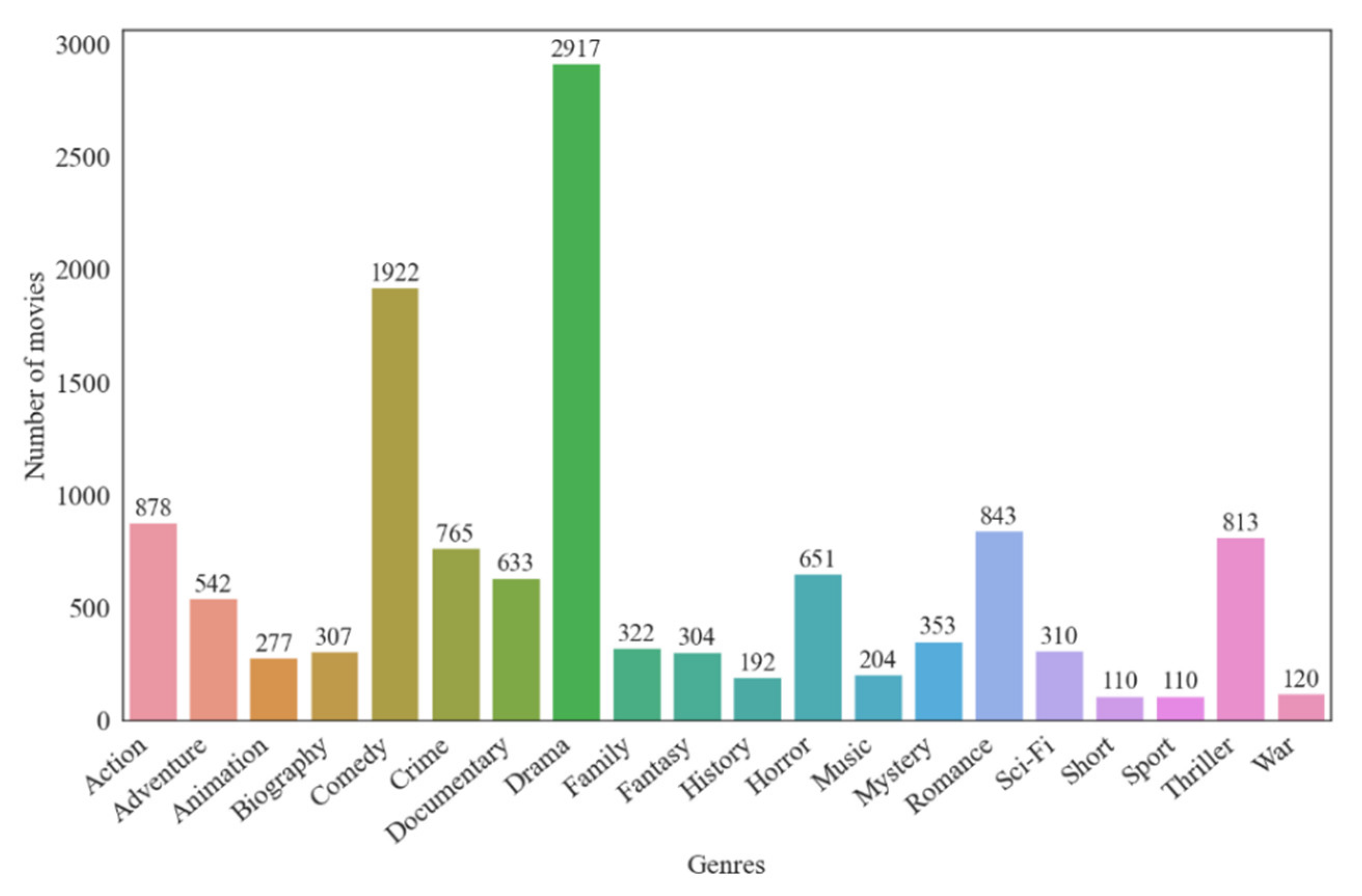
There were a total of 29,432 films in the dataset, comprising20 genres, each of which had more than 500 films from 1970 to 2018. The identified types are as follows: action, adventure, animation, biography, comedy, crime, drama, documentary, fantasy, family, history, horror, music, mystery, romance, sci-fi, short, sport, thriller, war. The distribution of the number of movies in each genre can be seen in Figure 1.

Figure 1. Distribution of the number of movies by genre.

As can be seen in Figure 1, the dataset is quite unbalanced regarding movie genres. It is well known that splitting imbalanced datasets as training and test sets is a challenging problem in multilabel classification tasks [28]. In general, random splitting techniques are used in a DL system. However, employing such a splitting technique causes underfitting in multilabel classification tasks. For this purpose, the method developed by Sechidis et al. [29] has been implemented and used to stratify our dataset. In this method, the initial unbalanced dataset was divided in k-fold. In each step, one fold is held for validation while other folds are used for training. The stratification step is repeated iteratively, until the criteria are met. At each iteration, the selected fold is also divided into sub-folds in which labels are distributed similar to the original dataset. These sub-folds are employed for training and validation at each iteration. After certain numbers of iterations, all sub-folds are combined to stratify the dataset.

The data were split as 80% and 20% as training and test, respectively. The stratification results can be seen in Figure 2 and Figure 3 which demonstrate the distribution of labels has been maintained.

Figure 2. Genre distribution of training set after iterative stratification.

Figure 3. Genre distribution of test set after iterative stratification.

To further explore the dataset, the number of genres for each poster/movie has been visualized in Figure 4. As can be seen in the figure, the majority of posters have multiple genres.

Figure 4. The distribution of movies which have multiple labels.

The iterative stratification method has also maintained the general distribution of the movies regarding the number of genres which can also be seen in Figure 4.

Genre values need to be converted to numeric values before multiclass classification. For this purpose, the genre variable was converted to a binary vector with dimension 20. Initially, all types are assigned 0. Whatever genre a movie belongs to is designated as 1. The process is called “multi-hot encoding”. As is known, the performance of deep-learning models is generally directly related to the number of data [30]. For this reason, random data augmentation was performed on the training data during the training of the models.

3.2. The Architecture of Pretrained Models

The use of a transfer-learning method has made a great contribution to developments in the field of deep learning. Transfer learning allows us to redesign models that were previously trained on very large datasets to solve our own problem. Training a model from scratch takes a lot of time and resources. Thanks to pretrained models, the training cost and time problems are overcome, and the problem is solved quickly and efficiently.

In the transfer-learning method, a pretrained model is used as a feature extractor. The top layers of the chosen pretrained model are removed to add new layers to adapt the model to the new task. According to this, the pretrained models mentioned above have been imported to the environment separately without the top layers. In order to provide a fair environment, identical dense layers have been appended to the top of the models.

Six of the modern pretrained models were selected for this task which were VGG16 [31], ResNet50 [32], InceptionV3 [33], DenseNet [34], MobileNet [35], and ConvNeXt [36]. The general structures of the used architectures are explained below.

VGG16 architecture, which was created with the principle of a small filter and deeper network, is a computer vision model that classifies 1000 different images in 1000 different categories in the field of image recognition and classification with 92.7% accuracy in the ImageNet Large-Scale Visual Recognition Challenge (ILSVRC) [37] held in 2014. The main motivation of the model is to examine the effect of increasing depth on classification accuracy. The successful results of the model prove that the motivation is correct. The architecture, which takes RGB images of 224 × 224 size as the input, consists of 16 convolutional layers, 3 fully connected layers, and the following softmax layer. Filters that are 3 × 3 filters with a stride of 2 are used in the convolutional layer. Filters that are 2 × 2 with a stride of 2 are used in the max pooling layers following some convolutional layers. The ReLU activation function is used after each convolutional and fully connected layer.

In order to solve more complex problems, the networks are made deeper. However, contrary to expectations, as the network depth increased, the training and test error rates also increased and the vanishing/gradient exploding problem occurred. The ResNet architecture, which proposes the residual block concept to overcome this problem, came first in the ILSVRC’15 competition held in 2015 with an error rate of 3.57%. Based on the VGG architecture, ResNet is eight times deeper than the VGG architecture but has lower complexity. The ResNet architecture consists of residual block stacks consisting of two convolutional layers with a 3x3 filter, batch normalization layer, and ReLU activation function. Residual block stacks facilitate the model to learn more complex and abstract features. The “skip connection” or “shortcut connection,” which lets the network skip one or more layers, is the main idea that these blocks explain. Thanks to this technique, the activations of one layer are linked to other layers by skipping some intermediates.

The InceptionV3 architecture is based on the main idea of wider networks rather than deepening networks for efficient feature extraction. It consists of repeating Inception modules with different dimensions. Each module consists of 1 × 1, 3 × 3, and 5 × 5 filtered convolutional layers. The primary concept involves the utilization of multiple filters with different sizes and the subsequent concatenation of their respective outputs. This facilitates the model in capturing features at varying spatial resolutions and acquiring diverse representations of the input. The InceptionV3 model employs global average pooling layers. This reduces overfitting and improves the generalizability of the model. The model integrates auxiliary classifiers at intermediate layers to mitigate the vanishing gradient problem during training. It employs factorization to reduce the computational cost by substituting large convolutions with a combination of smaller convolutions. Batch normalization is utilized by InceptionV3 to stabilize and expedite the training process. The model completed the ILSVRC’15 competition with a top five error rate of 3.58.

The DenseNet architecture, in which each layer in the network is connected with all other layers, is presented as a model that allows for the reuse of features, has fewer parameters, and is easy to train. For each layer in the network, the feature maps of the previous layers are used as the input and the combined feature maps are sent as the input to the next layer. Combining feature maps increases the diversity and efficiency of the inputs. The architecture generally consists of dense block, transition, and classification layers. In a dense block layer, a layer is directly connected to all subsequent layers. This is to improve the flow of information between layers. DenseNet employs bottleneck layers within dense blocks in order to reduce computational complexity. Typically, a bottleneck layer consists of a 1 × 1 convolution followed by a 3 × 3 convolution. Transition layer is the name given to the layers between two dense layers. This layer, which has a 1 × 1 convolutional layer and 2 × 2 avg pooling layer, changes the size of the feature map and reduces the spatial dimensions. The DenseNet architecture incorporates a hyperparameter referred to as the “growth rate,” which governs the quantity of additional feature maps generated by each layer. When the architecture was evaluated using four benchmark datasets, it was seen that it required a higher performance and fewer parameters than the previous architectures.

The MobileNet architecture is a model designed for mobile and embedded vision applications, which has proven successful in many applications in the field of computer vision. MobileNets take advantage of depthwise separable convolutions to build smaller and accelerate deep neural networks. A depthwise separable convolution consists of depthwise convolution and pointwise convolution. The depthwise convolution applies a single convolutional filter to each input channel individually. When compared to conventional convolutions, in which each input channel is combined with all of the filters, the computational cost of this method is greatly reduced. The pointwise convolution operation involves the application of a 1 × 1 convolution to the output obtained from the depthwise convolution. It allows the model to capture complex spatial patterns by mixing and combining the channels. The model consists of a total of 28 layers, including depthwise and pointwise. After each layer, batch normalization and ReLU layer were used. The network is completed with a fully connected and softmax layer.

The ConvNeXt model which is proposed by [36] exhibits enhanced accuracy, performance, and scalability compared to vision transformers, while retaining the design simplicity characteristics of convolutional neural networks. The effectiveness of conventional ConvNets is preserved by ConvNeXt, which also features a fully convolutional nature for both training and testing, making it very easy to put into practice. The group that created ConvNeXt progressively modernized the ResNet architecture in stages so that it can accommodate the building of a hierarchical vision transformer. Adjustments made with the aim of modernizing are grouped under the headings of macro design, ResNeXt, inverted bottleneck, large kernel size, and micro design. The details of the modernizing ResNet to ConvNeXt adjustments are as follows:

• The compute ratio of ConvNext is set to (3:3:9:3). The ConvNext architecture consists of four stages. Stage one, two, and four consist of three blocks and stage three consists of nine blocks.
• A 4 × 4 with a stride of four non-overlapping convolution “patchify stem” is used in the ConvNext architecture. Since the kernel size and stride size are the same, the patches do not overlap.
• The ConvNeXt architecture incorporates an inverted bottleneck block design, which shares similarities with existing models but introduces layer normalization and Gaussian Error Linear Units (GELU) activation as additional components.
• In ConvNeXt, a 7 × 7 with an increased kernel size depthwise convolutional layer is used in each block. Rearrange the order of the layers in the block such that the depthwise convolutional layer is positioned as the first layer.
• The number of activation functions and normalization layers are reduced in the ConvneXt architecture. The Rectified Linear Units (ReLU) activation function is replaced with the GELU activation function. The model uses a single GELU before a 1 × 1 convolutional layer in each block. Batch normalization (BN) has been replaced by layer normalization (LN).
• ConvNeXt uses separate downsampling layers between stages. These layers have layer normalization and a 2 × 2 convolutional layer with a stride of 2.

Several crucial components that contribute to the observed performance disparity are identified during the course of their investigation. The ConvNeXt architecture and its blocks can be seen in Figure 5 and Figure 6, respectively.

Figure 5. Architecture of the ConvNeXt model.

Figure 6. Design of the ConvNeXt block.

The general structure of a model used in the study is shown in Figure 7. The pretrained model is loaded into the system with weights but without the classification layers. This pretrained model will be used as the feature extractor. As mentioned before, all the models used here have previously produced very successful results in image classification and their feature extraction power has been proven. But the top layers of these models are suitable for the problem they were trained for before. For this reason, the top layers are not included. The output of the last layer before the fully connected layer is used as the input for our classifier. All the layers are frozen in order to prevent weight changes in the models with the new data. If the weights in these layers change, there is no difference compared to training the model from scratch. After this phase, fully connected layers suitable for our problem are appended.

Figure 7. General architecture of the models.

As mentioned above, six different pretrained models, which are described in general terms, VGG16, InceptionV3, Resnet50, MobileNet, DenseNet, and ConvNeXt, are used in this study. The input size of all the pretrained models was set up as 256 × 256. As can be seen in Figure 7, 1,024,512, 256,128, and 20-neuron fully connected layers are employed, respectively. All fully connected layers except the final layer include ReLU activation functions. On the other hand, the output layer has a Sigmoid activation function which is a necessity for multilabel classification problems. Also, batch normalization layers have been added between the fully connected layer to handle the overfitting problem.

3.3. The Evaluation Metrics

The final results and performance of the pretrained models are demonstrated using evaluation metrics, namely accuracy, loss, precision, F1-score, Hamming loss, and AUC. The accuracy, precision, and F-score are defined in Equations (1)–(3).

$$Accuracy=\frac{\mathrm{T}\mathrm{P}+\mathrm{T}\mathrm{N}}{\mathrm{T}\mathrm{P}+\mathrm{T}\mathrm{N}+\mathrm{F}\mathrm{P}+\mathrm{F}\mathrm{N}}$$

(1)

$$Precision=\frac{\mathrm{T}\mathrm{P}}{\mathrm{T}\mathrm{P}+\mathrm{F}\mathrm{P}}$$

(2)

$$F-score=\frac{2\times Precision\times Recall}{Precision+Recall}$$

(3)

Here, TP (true positive) is the number of instances correctly predicted as positive, TN (true negative) is the number of instances correctly predicted as negative, FP (false positive) is the number of instances incorrectly predicted as positive, and FN (false negative) is the number of instances incorrectly predicted as negative.

Accuracy (Equation (1)) can be defined as the proportion of correct classifications to the total number of predictions. Precision (Equation (2)) is the proportion of TP predictions to the total number of positive predictions. To calculate the F-score, recall must also be defined. Recall is the proportion of TP predictions to the positive instances on the dataset. The F-score (Equation (3)) is the harmonic mean of the precision and recall metrics.

For the loss metric, binary cross-entropy loss has been employed. This loss function is applicable for not only binary classification tasks but also multilabel classification tasks. It evaluates the dissimilarity between the predicted probabilities of positive labels and actual labels.

Hamming loss measures the percentage of labels that are incorrectly predicted over all samples in the dataset and it is defined as Equation (4). Hamming loss offers an evaluation of how well the model performs in correctly classifying each sample for all its relevant labels.

$$HammingLoss=\frac{Numberofincorrectlypredictedlabels}{Totalnumberoflabels}$$

(4)

The last metric is AUC which stands for area under the receiver operating characteristic curve (ROC). To define the AUC, the ROC curve must be explained. The ROC curve is the depiction of the performance of the model across different thresholds. The ROC curve plots a graphic with the TP rate against the FP rate with different values of thresholds. The AUC score is the area under this ROC curve and it demonstrates the distinguishing power of the model among classes. The AUC score can be between 0 and 1. An AUC score over 0.5 is interpreted as the model having performed better than random guessing. If the AUC score is close to 1, it can be interpreted as it categorizes almost perfectly.

4. Experimental Results and Discussion

All experiments were conducted on a desktop computer with the following specifications: Intel i7 7700K 4.20 Ghz CPU, Nvdia GeForce 1080 GPU, 16 GB RAM. This system has been developed using Python and its deep-learning frameworks Tensorflow and Keras. The pretrained models were obtained using the Keras library. As an optimization algorithm, Adam was used with a 0.001 learning rate. Binary cross-entropy loss was chosen as a loss function. The mini batch size and epoch number were determined as 32 and 10, respectively.

In the first stage of evaluation, all the layers of the pretrained models were frozen to avoid weight change. Only the new appended layers were unfrozen to ensure these fully connected layers were trained to solve the specific problem. A five-fold cross validation was used to choose the best hyperparameters. Each fold consisted of 10 epochs to train the model. The model with the best result was chosen for the second stage.

In the second stage of this study, the fine-tuning process, which included unfreezing all layers of the models and training them, was carried out. This unfreezing operation provided the opportunity to train the whole model from the top to bottom. The same dataset was used for the fine-tuning phase and the results were recorded.

In the final stage, the test images which were previously unseen by the model were used to evaluate the performance of the models. The accuracy metric alone is not sufficient for multilabel classification problems. Therefore, the F1-score, precision, recall, and AUC score were also used in addition to the accuracy. It is also worth mentioning that the 256 × 256 pixel image with the RGB channel was used as an input for each model.

In the remaining part of this section, the outcomes of this study are presented. To keep the figures simple, only the training results of the two best models (ConvNeXt and DenseNet) are demonstrated.

Figure 8 shows the accuracy score of the training process of the ConvNeXt and DenseNet models which includes the training and test accuracy scores over the epochs. In the training process base models, which include the pretrained feature extraction, parts of the models are frozen and only the dense layers on top are trained. As a result of this, the training and validation accuracy follow quite similar paths in the figure. As can be seen in the figure, the accuracy results reached over 90% in the training phase.

Figure 8. Training accuracy of ConvNeXt and DenseNet models over the epochs.

The training loss of the two aforementioned models can be seen in Figure 9. For the reasons explained above, the loss values also proceed similarly for the two models, reaching below 27%.

Figure 9. Training loss of ConvNeXt and DenseNet models over the epochs.

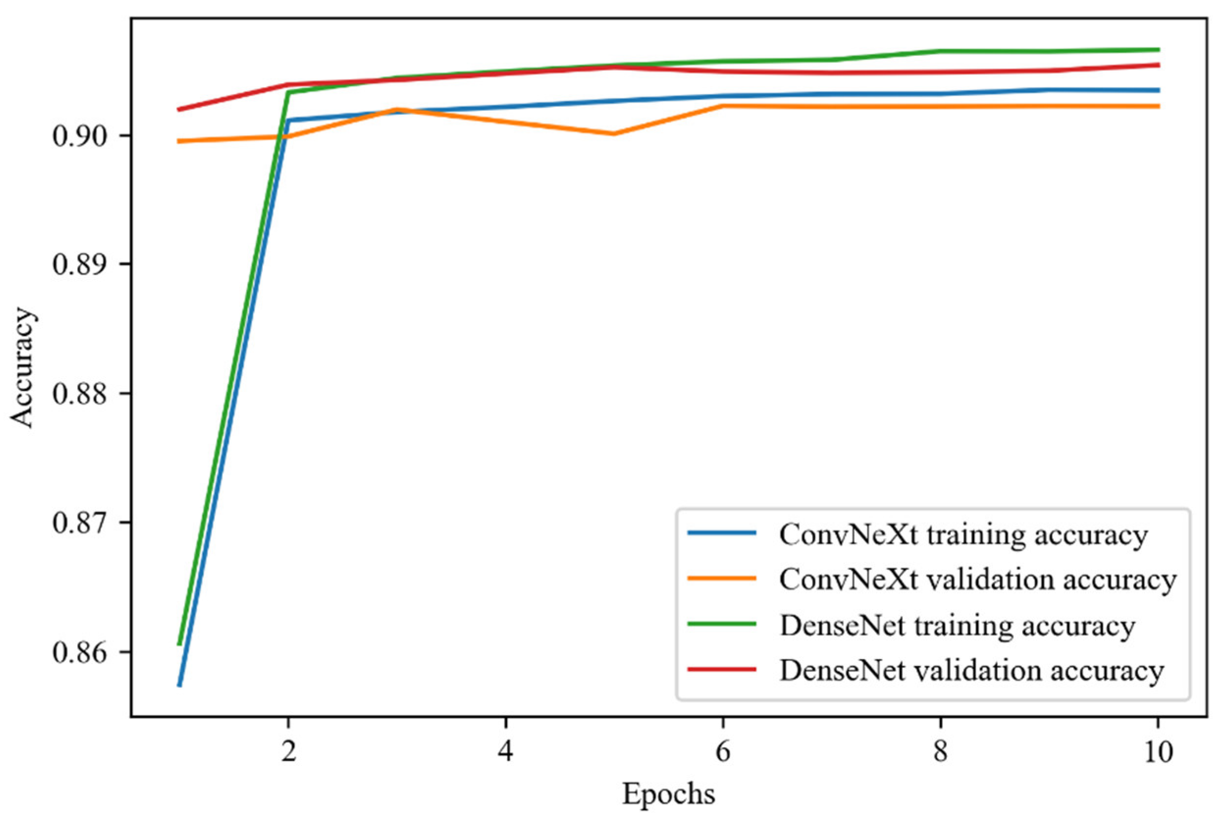
In Figure 10, the accuracy scores through each epoch of the fine-tuning phase for both pretrained models can be seen. The accuracy of both models reached above 90% accuracy for the fine-tuning phase. As the epochs passed, the training accuracy of DenseNet increased but the validation accuracy decreased which can be a sign of overfitting. On the other hand, ConvNeXt demonstrated a different performance. Not only the training but also the validation accuracy increased in each epoch which can be the sign that the model fits well for the problem.

Figure 10. Fine-tuning accuracy of ConvNeXt and DenseNet models over the epochs.

For the fine-tuning phase, the loss graph over epochs, which can be seen in Figure 11, also supported the results of the accuracy metrics. While both loss scores of ConvNeXt decreased, the validation loss score of DenseNet increased.

Figure 11. Fine-tuning loss of ConvNeXt and DenseNet models over the epochs.

In the final stage of this experiment, the test of the models with the previously unseen test images was performed. The results of the test phase can be seen in Table 2. Although the accuracy outcome is quite similar on each model, DenseNet has yielded the best result. The performance of ConvNeXt, which is the novel model for this problem, is excellent overall. The accuracy of the ConvNeXt model is 90.45% which is the second-best performance after DenseNet. InceptionV3 is another model that reached over 90% accuracy. The weakest performance among the models is demonstrated by MobileNet and ResNet, yet the score is above 89%.

Table 2. Results of evaluation regarding metrics on pretrained models.

Models	Accuracy	Loss	Precision	Hamming Loss	F1-Score	AUC
VGG16	0.9021	0.267	0.3365	0.0976	0.4042	0.748
MobileNet	0.8963	0.6706	0.3166	0.1023	0.3822	0.7345
InceptionV3	0.9008	0.2912	0.3244	0.0989	0.3932	0.7445
DenseNet	0.9058	0.2615	0.3585	0.0936	0.4302	0.7671
ResNet	0.8999	0.2744	0.3026	0.1023	0.3688	0.728
ConvNeXt	0.9045	0.2598	0.3310	0.0971	0.4028	0.7538

The pretrained models produced a different range of loss results in this study. The ConvNeXt model is the overachieving one among the pretrained models with a 25.98% score. Also, the loss score of DenseNet is close to the ConvNeXt model. VGG16 produced a less than 27% loss score. While InceptionV3 displayed a 29.12% loss score, the most dramatic score in the table was generated by MobileNet with 67.06%. The reason for this poor loss result for MobileNet arises from the fact that the input shape of 256 × 256 is not suitable for it.

Regarding precision, the models generated scores about between 30% and 36%. DenseNet, again, generated the best results with 35.85%. VGG16 was the second-best model regarding precision. The ConvNeXt model generated a 33.1% precision score which is slightly less than the score of VGG16.

The performance of DenseNet is again the best one regarding the Hamming loss with 9.89%. ConvNeXt demonstrated the third-best result after the VGG16 model. InceptionV3 is one of the models that produced less than a 10% Hamming loss. MobileNet and ResNet displayed similar results for this metric.

Table 2 also provides the F1-scores in which DenseNet demonstrated the best result with a score over 43% which is the best score by far. ConvNeXt and VGG16 reached a score over 40%. The weakest performance was produced by ResNet.

The last metric on the table is the AUC which also supports the dominance of DenseNet. ConvNeXt is the second model which reached an AUC score above 75%. ResNet demonstrated the weakest performance regarding this metric.

The confusion matrix of the novel model for this problem, ConvNeXt, can be seen in Figure 12. The multilabel nature of the problem makes it difficult to show in a conventional confusion matrix. Yet, it can be demonstrated in the way of the corresponding figure. The number indicated as 0 indicates all labels except the label present in that sub-figure. The numbers up to 19 represent the label present in the sub-figure. In the figure below, the drama and comedy labels draw attention. A total of 1426 comedy-labeled and 2537 drama-labeled movies were correctly classified. On the other hand, history, sport, music, and war-labeled movies were not predicted well which is caused by the few numbers of movies in the aforenamed genres.

Figure 12. Confusion matrix of ConvNeXt model.

The comparison of the genre prediction of ConvNeXt, with the actual genre of the same movie on IMDB, is shown in Figure 13 below. As can be seen in the figure, three posters from movies that aired in 2022 have been used for the test and the model demonstrates satisfactory results. The Top Gun Maverick movie has two labels, namely action and drama which are in the top three predictions of the model. The Batman movie, on the other hand, has three labels. The ConvNeXt model correctly predicted the action label with 89%. However, the second predicted label does not exist in the labels for the movie. Drama is predicted as the fourth possible label. The last movie in the figure is Senior Year which has comedy and drama labels which are correctly predicted by the model.

Figure 13. Comparison of prediction of ConvNeXt and ground truth IMDB genres.

5. Conclusions

In recent years, advancements in deep learning, computer vision, and natural language processing have revolutionized the field of the multilabel classification of movie posters. Researchers and data scientists have explored various approaches, including convolutional neural networks (CNNs), transfer learning, ensemble methods, and hybrid models that combine image analysis with textual information extracted from the posters’ accompanying metadata. These techniques leverage large-scale labeled datasets, encompassing vast collections of movie posters and their corresponding genre labels, to train models that generalize well and exhibit a high predictive accuracy.

The potential applications of the multilabel classification of movie posters extend beyond the realms of film production and distribution. Streaming platforms can leverage these models to enhance their recommendation systems, suggesting movies to users based on their preferred genres. Movie enthusiasts can explore diverse genres and discover hidden gems that align with their cinematic preferences. Filmmakers and marketers can gain valuable insights into genre trends, enabling them to tailor promotional campaigns and target specific audience segments effectively.

In conclusion, the multilabel classification of movie posters based on genre is an exciting research area that combines the realms of computer vision, machine learning, and film aesthetics. It enables us to unlock the visual cues embedded within movie posters and automatically assign genre labels, providing a deeper understanding of films and empowering various stakeholders in the film industry. With the continued advancements in machine learning and the availability of comprehensive movie poster datasets, we can expect further breakthroughs in this field, ultimately enhancing our movie-watching experiences and broadening our cinematic horizons.

In this study, our aim was to classify the movie posters based on genres which is a challenging problem considering most of the movies have two or three genres. Also, the imbalanced genre distribution of the dataset makes the problem more and more difficult to overcome. For this purpose, we used binary cross-entropy loss which alleviated the challenging effect of the imbalanced dataset. In the training section, we used five-fold cross-validation to find the best hyperparameters. We also employed a novel pretrained model, ConvNeXt, for this problem and compared the results with the former pretrained models. The evaluation stage yielded promising results and the performance of the ConvNeXt model is satisfactory regarding the metrics. This study demonstrated the power of the novel pretrained model on the multilabel classification problem.

As for future work, the dataset will be expanded with modern movie posters and we believe that ConvNeXt will provide a better performance. Also, the domain of the study will be broadened using the plot summaries and state-of-the-art natural language-processing techniques. The results of both techniques will be evaluated, and the final prediction will be decided. With this addition, we believe the results can be improved and used for other multilabel classification problems.