Deep Learning Models for Quantitative Precipitation Estimation Based on Weather-Radar and Rain-Gauge Datasets

Abstract

Quantitative precipitation estimation (QPE) is a fundamental task of hydrometeorological applications, ranging from flash-flood detection to water-resource management. While weather radars offer superior spatial coverage compared with rain gauges, traditional estimation based on the empirical $Z-R$ (reflectivity factor vs. rainfall rate) relationship fails to capture spatial variability and tends to underestimate extreme rainfall. The idea pursued here is to learn the radar-to-rainfall mapping by means of a convolutional neural network (CNN) trained on co-located radar and rain-gauge data; thus, once trained, the network can convert radar reflectivity measures into rainfall values, even where gauges are unavailable. Although machine learning techniques are promising for this task, they typically demand large training sets. To operate in a limited-data regime, we introduce a U-Net architecture that separates the analysis of space from that of time: each block first looks at the structure of the reflectivity field and then at how it changes over consecutive radar scans, extracting spatiotemporal features from volumetric data with fewer parameters than a full three-dimensional filter. The model is evaluated on a severe convective event that affected Tuscany, Italy, on 2 November 2023, benchmarking its performance against the classical Joss–Waldvogel $Z-R$ relationship (suitable for convective events), a data-driven log-regression of weather-radar and rain-gauge data, and a baseline CNN architecture. The main advantages are negative bias—i.e., underestimation of rainfall—more than halved and correlation with rain-gauge measures more than doubled, under the same operational conditions. What is noteworthy is the capability of learning the model from radar and rainfall data taken in different times and places, as well as the possibility of converting a reflectivity map into a rainfall map without the need for simultaneous rain-gauge measures. This is an asset of fixed parametric methods; however, they are far less accurate.

1. Introduction

Reliable quantitative precipitation estimation (QPE) plays a central role in modern hydrometeorology because many operational activities depend on timely and spatially distributed rainfall information. Accurate precipitation fields are essential for flash-flood warning systems, river-flow forecasting, hydraulic risk assessment, water-resource management, agricultural planning, climate monitoring, and several industrial applications [1]. The increasing frequency of short-duration, high-intensity precipitation events has further emphasized the need for estimation techniques capable of providing both high spatial resolution and high quantitative accuracy.

Operational QPE mainly relies on two complementary observation systems: rain gauges and weather radars. Rain gauges provide direct measurements of precipitation and constitute the reference source for rainfall observations. Their main limitation is the sparse spatial sampling imposed by practical and economic constraints. Even relatively dense monitoring networks may fail to describe the highly localized structure of convective precipitation, while measurement uncertainties caused by wind effects, shielding, instrument malfunction, or missing observations further complicate the reconstruction of continuous rainfall fields [1,2,3]. Consequently, rainfall maps derived exclusively from rain-gauge observations require spatial interpolation techniques, ranging from deterministic methods such as inverse-distance weighting to geostatistical approaches including kriging [4,5,6,7]. Although these techniques are effective under smoothly varying precipitation conditions, their performance rapidly deteriorates when intense rainfall exhibits strong spatial gradients.

Weather radars address this limitation by continuously monitoring precipitation over wide areas with kilometer-scale spatial resolution and revisit times of only a few minutes [8]. Their capability of capturing the spatial organization and temporal evolution of precipitation makes them indispensable for real-time monitoring of severe weather. Radar observations, however, do not directly measure rainfall intensity. Instead, they estimate the electromagnetic backscattering produced by hydrometeors, from which rainfall must be inferred through physical or empirical models. The resulting estimates are affected by several uncertainty sources, including attenuation, beam blockage, ground clutter, calibration inaccuracies, and errors associated with Doppler processing [9,10,11]. Consequently, despite their excellent spatial coverage, radar-derived rainfall products often exhibit systematic and local biases.

The conversion from radar reflectivity to rainfall rate is traditionally based on empirical reflectivity–rainfall relationships of the form

$$Z=a{R}^b,$$

(1)

where Z denotes the radar reflectivity factor and R the rainfall rate [12]. The coefficients a and b depend on the drop-size distribution (DSD), whose characteristics vary with precipitation type, geographical location, and atmospheric conditions [9,13,14]. Since these coefficients are rarely constant during real precipitation events, the adoption of fixed parameterizations frequently introduces significant estimation errors [15,16]. Although numerous $Z-R$ relationships have been proposed for different climates and radar systems [17,18,19,20], no universal parameterization is capable of accurately describing the large variability encountered in operational scenarios.

The introduction of dual-polarization weather radars has significantly improved radar-based precipitation retrieval. Polarimetric variables, including differential reflectivity, differential phase, and specific attenuation, provide additional information on hydrometeor characteristics and permit a more accurate characterization of precipitation microphysics [21,22,23]. These measurements enable adaptive rainfall algorithms that partially compensate for attenuation and improve the estimation of rainfall intensity [24,25,26]. Nevertheless, even advanced polarimetric techniques remain indirect measurement methods and cannot completely eliminate the uncertainties associated with observing precipitation at considerable distances and elevations above the ground [27].

These limitations have motivated the development of approaches that exploit the complementary characteristics of radar observations and rain-gauge measurements. Rather than considering the two sensors independently, recent research has increasingly focused on combining their information to improve the spatial representation of rainfall while preserving quantitative accuracy. Existing fusion strategies can be broadly classified into three families according to the role assigned to each observation system during the estimation process [27].

Existing fusion techniques differ in the ways in which radar observations and rain-gauge measurements are combined. Geostatistical approaches use rain gauges as the primary source of quantitative information while exploiting radar observations as auxiliary variables to improve spatial interpolation. Representative examples include kriging with external drift (KED) and conditional merging (CM), which have consistently demonstrated superior performance over conventional interpolation techniques under a wide range of precipitation conditions [5,27,28,29]. A second class of methods attempts to compensate for radar biases by estimating multiplicative or additive correction factors from rain-gauge observations. Mean Field Bias (MFB), Brandes Spatial Adjustment (BSA), and more recent adaptive formulations based on space–time calibration of the $Z-R$ relationship belong to this category [12,30,31,32,33]. Finally, probabilistic integration techniques, including co-kriging and Bayesian merging, estimate rainfall by explicitly combining the uncertainties associated with each observation system [27,34,35]. Although these methods generally improve the quality of radar-only estimates, they still rely on predefined statistical assumptions and require the availability of rain-gauge observations during the estimation stage.

The growing availability of large radar archives and the remarkable progress achieved in machine learning have recently stimulated the development of data-driven approaches for precipitation estimation. Instead of explicitly modeling the physical relationship between radar measurements and rainfall, these methods learn it directly from observations. Deep neural networks have demonstrated excellent performance in numerous Earth-observation applications thanks to their capability of extracting complex spatial and temporal patterns from large datasets [36,37]. Their application to precipitation estimation has therefore received increasing attention during the last decade [38,39].

Several studies have demonstrated the potential of deep learning for QPE. Chen et al. [40] proposed a two-stage neural architecture that exploits a ground-based radar to bridge the relationship between spaceborne radar observations and rain-gauge measurements. Moraux et al. [41] developed a deep learning framework combining satellite observations and rain gauges for rainfall retrieval. More recently, convolutional neural networks and related machine learning models have been investigated using weather-radar observations, showing encouraging improvements over conventional empirical approaches [42,43,44]. Despite these promising results, many existing models require extensive training datasets collected over several years and often exhibit limited generalization when applied to geographical regions that are poorly represented during training. Moreover, the tendency of standard loss functions to favor the most frequent rainfall intensities frequently leads to an underestimation of localized extreme precipitation—precisely the situations of greatest operational interest.

The present work addresses these limitations by investigating a deep learning framework specifically designed for situations where only limited training data are available. The proposed architecture is based on a U-Net backbone enriched with $(2+1)$D convolutional blocks, which separately model the spatial and temporal dimensions of the radar sequence in order to improve the extraction of spatiotemporal precipitation features. In addition, we investigate target-weighted loss functions that assign greater importance to high rainfall rates, thereby mitigating the systematic underestimation typically observed for severe precipitation events.

The proposed methodology is evaluated using weather-radar observations and rain-gauge measurements collected during the severe convective event that affected Tuscany (Italy) on 2 November 2023, considering radar sequences acquired between 30 October and 4 November 2023. The developed model is compared with a baseline convolutional neural network, four conventional fixed $Z-R$ relationships, and an event-specific data-driven $Z-R$ calibration. To assess the ability of the network to generalize beyond the instrumented areas used for training, the experimental validation adopts a province-level spatial partition combined with an anti-leakage buffer that prevents information sharing between training and testing regions.

The remainder of this paper is organized as follows: Section 2 describes the meteorological event, the radar and rain-gauge datasets, and the proposed neural architectures. Section 3 presents the experimental results and compares the proposed approach with both empirical and data-driven benchmark methods. Section 4 discusses the implications of the obtained results, highlighting the advantages and limitations of learning-based QPE under limited-data conditions. Finally, Section 5 summarizes the main findings and outlines possible directions for future developments.

2. Materials and Methods

2.1. Study Area and Data Sets

2.1.1. Meteorological Event Description

Technical details concerning the meteorological case study analyzed in this paper can be found in the official report provided by the LaMMA Consortium (Environmental Modeling and Monitoring Laboratory for Sustainable Development) [45].

During the afternoon of 2 November 2023, the passage of a quasi-stationary instability line ahead of an advancing cold front triggered widespread convective activity across Tuscany. The development of these thunderstorms was significantly amplified by a highly unstable atmospheric environment, characterized by an elevated convective potential energy capable of supporting strong, sustained updrafts, together with a high moisture content in the lower troposphere, which ultimately led to extreme localized precipitation.

Specifically, starting at 15:30 UTC, a marked low-level convergence zone was established between strong south winds and incoming north flow. This mechanical forcing, combined with the advection of cooler air aloft and favorable thermodynamic conditions in the boundary layer, favored the formation of a severe convective line. The phenomenon exhibited a nearly stationary behavior until approximately 20:30 UTC, geographically stretching from the coastal and central provinces of Livorno and Pisa, towards Pistoia, Prato, and Florence.

The spatial geo-localization, exceptional intensity, and persistent stationary nature of this storm system featured highly nonlinear dynamics, presenting severe challenges for operational weather forecasting. As a consequence of the heavy rainfall, several rivers and torrents overflowed, resulting in widespread environmental damage and severe impacts on local communities.

2.1.2. Weather-Radar Dataset

The radar observations analyzed in this study were acquired by the Italian national weather-radar network, operated by the Italian National Civil Protection Department (DPCN). The network comprises 26 radar systems, including 22 C-band and 4 X-band radars, the majority of which are dual-polarized, providing coverage of the entire Italian territory. The Tuscany region is covered by five C-band dual-polarization weather radars located in Tuscany and the neighboring regions:

• Monte Croce, Tuscany, province of Lucca, at 1307 m a.s.l.;
• Monte Settepani, Liguria, province of Savona, at 1390 m a.s.l.;
• Gattatico, Emilia Romagna, province of Reggio Emilia, at 34 m a.s.l.;
• San Pietro Capofiume, Emilia Romagna, province of Bologna, at 10 m a.s.l.;
• Monte Serano, Umbria, province of Perugia, at 1428 m a.s.l.

The raw data from all systems undergo synchronous scans every 5^′ and are processed by the DPCN, which applies several corrections for ground clutter, partial beam blockage, and attenuation, before generating national-scale mosaicked products. Some artifacts may persist, such as residual beam blockage effects or issues at the extreme edge of the coverage zones, which act as operational infrastructure factors that models must learn to handle.

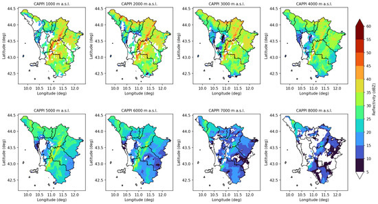
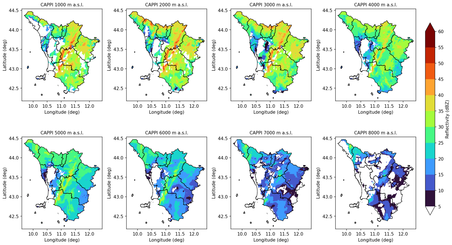
The observation period encompasses a multi-day interval (30 October 2023 through 4 November 2023), comprehensively framing the extreme rainfall event of 2 November. For this study, we selected the reflectivity products of the constant altitude plan position indicator (CAPPI). To fully capture the vertical structure and evolution of the precipitation, eight different CAPPI slices were extracted, spanning 1000 m to 8000 m altitude a.s.l. (above sea level). The data exhibit a horizontal spatial resolution of $1\times 1$ km² and were aggregated to a temporal repetition of 10^′. The volumetric radar input, from which DL estimators start, is illustrated in Figure 1, which shows the eight CAPPI reflectivity levels (1000 to 8000 m a.s.l.) at the peak of the event.

Figure 1. The eight CAPPI reflectivity levels (1000–8000 m a.s.l., in dBZ) from the radar volume acquired on 2 November 2023 at 21:00 UTC, with the Tuscany regional boundary and provincial borders overlaid. These fields constitute the volumetric input from which the rainfall maps of Figure 6 are produced by the two DL-based methods. Reflectivity values below 5 dBZ within the regional boundary are shown in white.

The vertical structure—intense reflectivity at low levels that decays with height—is available to deep models through the full cube, whereas the $Z-R$ parametric relationships use only a single reference level at 2000 m a.s.l. The first slice (0 to 1000 m) was discarded because the five weather radars that cover Tuscany are placed at a height greater than 1000 m or must image beyond mountains as high as 2000 m.

2.1.3. Rain-Gauge Dataset

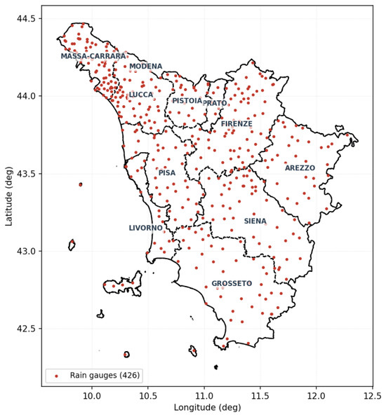
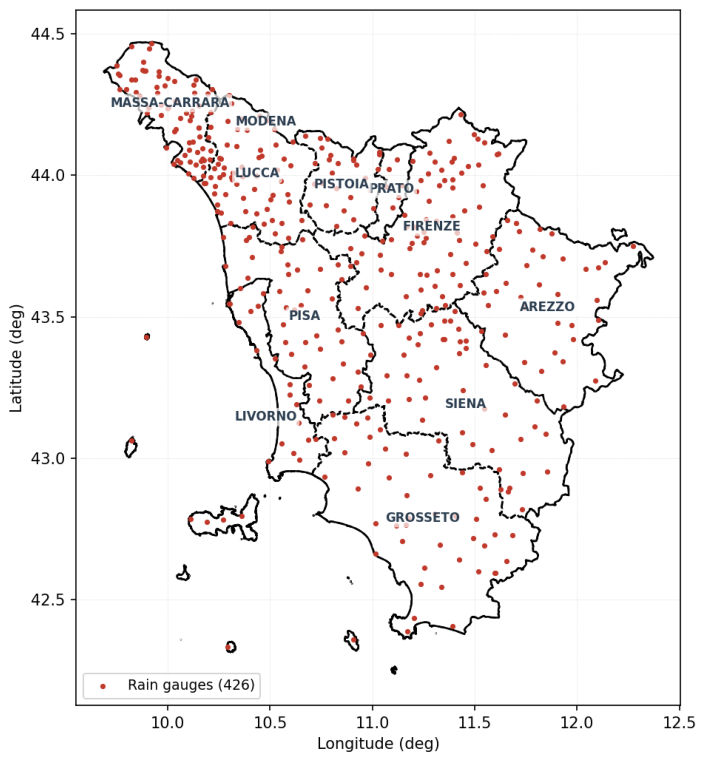
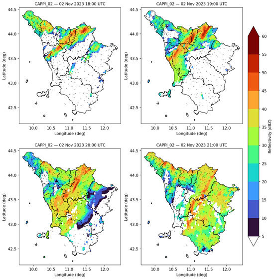
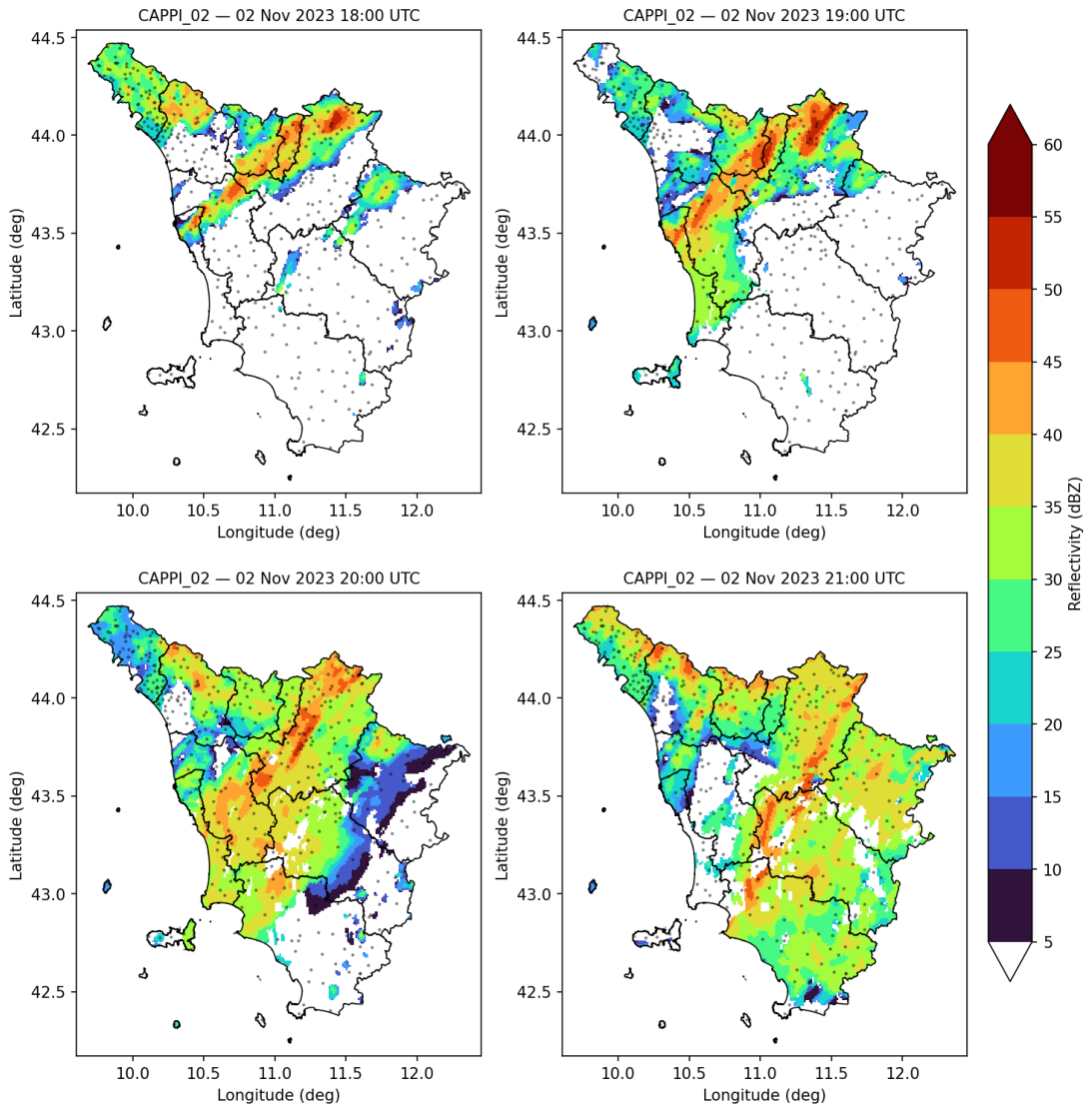
The ground-reference rainfall data was obtained from the regional rain-gauge network of Tuscany, operated by the LaMMA Consortium. The network comprises 426 tipping-bucket stations uniformly distributed across the regional territory of approximately 22,987 km², resulting in an average density of one gauge every 54 km². The spatial configuration and distribution of the active stations in the regional territory are shown in Figure 2. Four examples of the 2000 m a.s.l. CAPPI layers following the peak of the convective event, with the gauge network overlaid, are provided in Figure 3.

Figure 2. Spatial distribution of the regional rain-gauge network across Tuscany. Red dots indicate the locations of the tipping-bucket stations within the regional administrative boundary, providing the ground-reference data for the study area. Provincial boundaries and names are also shown, as they are referred to throughout the paper, particularly in the description of the dataset partitioning (Section 2.2.3).

Figure 3. CAPPI radar reflectivity product at a constant height of 2000 m a.s.l. captured at different timestamps on 2 November 2023: 18:00 UTC, 19:00 UTC, 20:00 UTC, and 21:00 UTC. The layout of Tuscany and provinces therein, with positions of rain gauges, is overlaid.

2.2. Setup

This subsection outlines the experimental configuration established to train and evaluate the proposed models. We first describe the preprocessing and temporal resampling of the ground-truth rain gauge records, followed by the integration protocol used to assemble the multi-dimensional spatiotemporal data cubes from radar and gauge data. Finally, we detail the spatial partitioning strategy implemented to ensure a robust evaluation across independent geographical domains.

2.2.1. Rain-Gauge Dataset Preprocessing

To temporally align gauge records with radar acquisitions, native 15 min precipitation accumulations were resampled at 10^′ intervals through a mass-conserving mathematical procedure. Any measure affected by instrumental errors or missing values was systematically discarded.

2.2.2. Data Integration and Spatiotemporal Cube Generation

To build the final test dataset, radar and rain-gauge data were spatially and temporally matched. For each active rain gauge, a $21\times 21$ pixel window (corresponding to an area of $21\times 21$ km²) centered on the geographical coordinates of the gauge was extracted from each of the eight CAPPI layers, resulting in an $8\times 21\times 21$ volumetric data cube.

To account for the short-term temporal evolution of the precipitating systems, six consecutive 10 min frames covering exactly a one-hour interval prior to the observation were stacked together. This procedure produced a comprehensive spatiotemporal hypercube $8\times 6\times 21\times 21$, which was then coupled with the cumulative hourly rainfall measured by the target gauge.

To focus the learning process on meaningful precipitation events, samples corresponding to null or negligible rainfall were filtered out. A spatiotemporal cube was retained only if the target hourly cumulative rainfall exceeded 0.5 mm and at least one radar pixel, across all spatial dimensions and elevation layers, registered a reflectivity greater than 10 dBZ.

Following these criteria, 411 rain gauges contributed at least one valid sample, resulting in a final dataset of 10,790 valid spatiotemporal cubes. The extreme nature of the event is confirmed by the target hourly rainfall distribution, which reaches peaks up to approximately 87 mm, while the rain gauges span a wide topographical range of elevations from sea level up to 1700 m a.s.l.

2.2.3. Dataset Partitioning

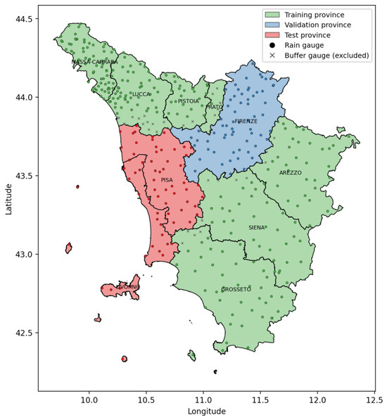
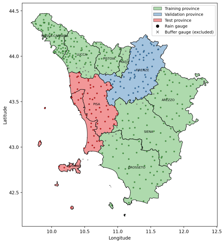
A purely random partition of the samples would be inappropriate for this task: since the data are point-based and spatially auto-correlated, a model could attain a high score simply by interpolating between gauges that are close to others seen during training, thereby overestimating its true skill on ungauged areas. To evaluate genuine spatial generalization, we therefore adopt a spatially blocked partition at the province level: entire provinces are held out, so that every test gauge lies in a region never observed during training (see Figure 4). The provinces of Pisa and Livorno, which were hit hardest by the convective line (Section 2.1), constitute the test set (67 gauges, 978 radar samples); the province of Florence is used for validation (62 gauges, 1288 samples); and the remaining provinces form the training set (282 gauges, 8524 samples). Gauges are assigned to provinces by a point-in-polygon intersection with the administrative boundaries. Province blocking removes interpolation across most of the domain, but test gauges lying close to a province border may still have training gauges within their $21\times 21$ km² input window, which would reintroduce a residual, “soft” form of leakage. To eliminate this, we enforce an anti-leakage spatial buffer: every training gauge located within 10.5 km, half the size of the largest input window—i.e., the patch radius—of a validation or test gauge, is discarded. Distances are computed as haversine distances between gauge coordinates. The buffer is applied on the training side, so that the held-out sets remain intact: it discards 34 training gauges (740 samples, ≈9% of the training data, thereby reducing it from 8524 to 7784 samples), while the test set and the validation set are unchanged. Because the same buffer is used for every input-window size, the test set is identical throughout the experiment; by construction, no training gauge ever falls inside the footprint of a test gauge. This makes the evaluation in Section 3.2 robust to interpolation leakage, at the cost of a more demanding test set (the heavy-rain coastal provinces), which explains the larger absolute errors compared to a random partition.

Figure 4. Province-level spatially blocked partition of the Tuscany rain-gauge network. Entire provinces are held out: Pisa and Livorno form the test set (red), Florence is used for validation (blue), and the remaining provinces constitute the training set (green). Colored dots indicate the rain gauges retained in each split; gray crosses are the training gauges discarded by applying a 10.5 km anti-leakage buffer around validation and test gauges.

2.3. Deep Learning Models

To investigate possible advantages of the nonparametric DL approach, we implemented two distinct architectures and compared them on the test dataset.

2.3.1. Network Models

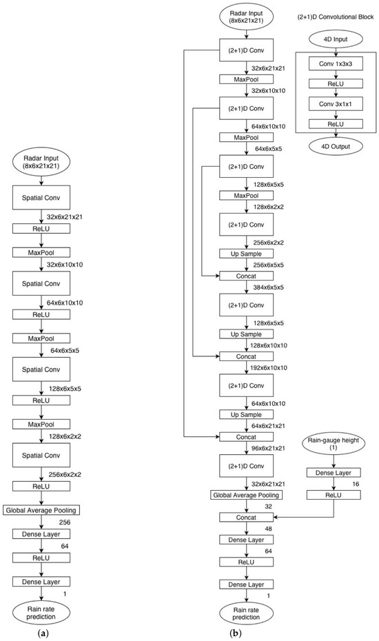
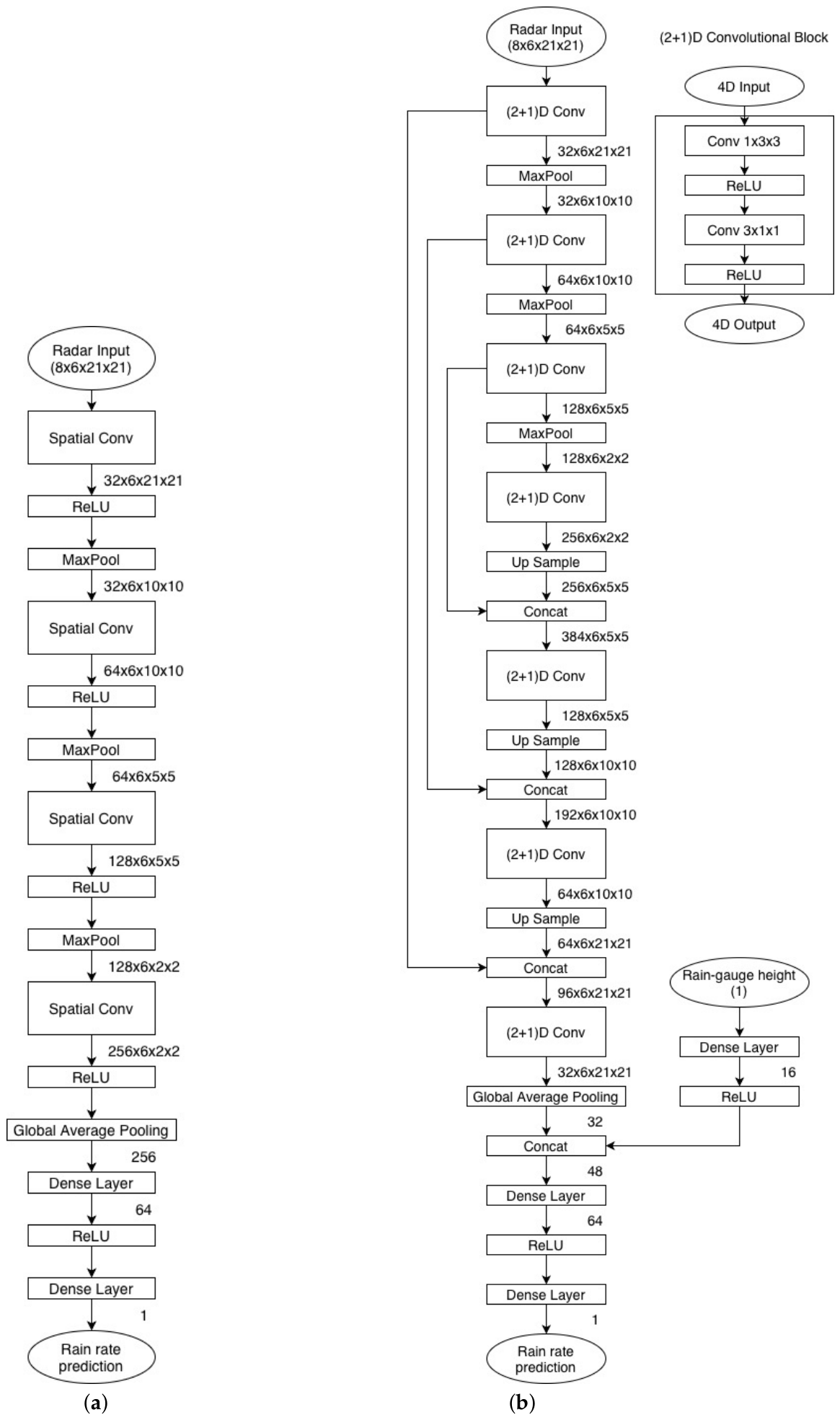
The first architecture serves as a baseline CNN and consists of four sequential feature extraction blocks. The network is shown in Figure 5a. It employs convolutional kernels of size (1,3,3), progressively increasing the number of feature channels while reducing the spatial resolution through max pooling [46]. At the end of the network, a global average-pooling layer generates a 256-element feature vector, which is projected to a 64-element representation vector and finally mapped to the output through two fully connected layers.

Figure 5. Flowcharts of learning models: (a) baseline spatial CNN; (b) proposed $(2+1)D$ U-Net model integrating radar sequences with rain-gauge elevation data.

The second architecture adopts a U-Net core, enhanced through $(2+1)D$ convolutional blocks. The U-Net architecture was selected for its proven ability to handle limited datasets effectively [47]. Furthermore, $(2+1)D$ convolutional blocks were adopted because they have been demonstrated to provide superior results compared to standard 3D convolutions when processing data characterized by temporal evolution [48]. The model is depicted in Figure 5b. The $(2+1)D$ block explicitly decomposes the 3D convolution into separate spatial (1, 3, 3) and temporal (3, 1, 1) convolutions to better capture complex spatiotemporal dependencies. The U-Net encoder is made up of four layers. As in the baseline CNN, the number of channels grows and the spatial resolution decreases when we go deeper into the encoder structure. The decoder uses classical U-Net skip connections and upscales the encoder output. A global-average-pooling layer flattens the output of the U-Net into a 32-unit layer, to which the altitude a.s.l. of the rain gauge is added as extra information. The two final layers reduce the output of the network to a scalar.

2.3.2. Loss Functions

Both architectures were trained using either mean absolute error (MAE) or mean squared error (MSE) as loss functions, which are commonly employed for regression tasks in deep learning. They are defined as

$$\begin{array}{cc}\hfill \mathrm{MSE}& ={\displaystyle \frac{1}{N}}{\displaystyle \sum _{i=1}^N}{({\widehat{y}}_i-y_i)}^2\hfill \\ \hfill \mathrm{MAE}& ={\displaystyle \frac{1}{N}}{\displaystyle \sum _{i=1}^N}|{\widehat{y}}_i-y_i|\hfill \end{array}$$

(2)

where N denotes the number of samples, $y_i$ represents the observed value (ground truth), and ${\widehat{y}}_i$ is the predicted value. Usually, $\mathrm{RMSE}\triangleq \sqrt{\mathrm{MSE}}$ is used for comparisons, having a homogeneous scale with MAE.

To correct the systematic underestimation of intense rainfall, we also trained the two networks with target-weighted variants of the losses (wMSE, wMAE), in which each sample is weighted by a function of its target value:

$$\begin{array}{cc}\hfill \mathrm{wMSE}=& {\displaystyle \frac{1}{{\sum }_i{w}_i}}{\displaystyle \sum _{i=1}^N}{w}_i{({\widehat{y}}_i-y_i)}^2\hfill \\ \hfill \mathrm{wMAE}=& {\displaystyle \frac{1}{{\sum }_i{w}_i}}{\displaystyle \sum _{i=1}^N}{w}_i|{\widehat{y}}_i-y_i|\hfill \end{array}$$

(3)

with $w_i=1+\lambda y_i$ and $\lambda =1$. The weights are normalized so that their mean is one; thus, the loss scale is kept comparable to the unweighted version and reduces to plain RMSE/MAE for $\lambda =0$. Heavier-rain samples thus contribute more to the loss.

3. Results

3.1. Benchmarking

As parametric estimators for reference, we used four classical reflectivity–rainfall relations of Equation (1), which differ only in the choice of coefficients a and b:

1.

Marshall–Palmer [17], widespread for stratiform precipitation: $a=200$, $b=1.6$;

2.

Joss–Waldvogel [18], suitable for convective events: $a=300$, $b=1.5$;

3.

Multi-Radar Multi-Sensor (MRMS) [19], for convective regimes: $a=300$, $b=1.4$;

4.

Rome C-band [20], specific to C-band radars: $a=519$, $b=1.64$.

To quantify how much can be gained by tuning the power law to the event itself, rather than adopting coefficients from the literature, we included a data-driven parametric method, in which the coefficients a and b of Equation (1) are not prefixed but are estimated from the training rain gauges by a logarithmic regression between reflectivity, averaged over a one-hour period and a 3×3 window of radar cells, and the corresponding measured hourly rainfall:

$$log\left(R\right)=1/b·[log\left(\overline{Z}\right)-log\left(a\right)]=1/b·log\left(\overline{Z}\right)-{\displaystyle \frac{log\left(a\right)}{b}}$$

(4)

in which $\overline{Z}$ is the $3\times 3$ spatial average of Z averaged over an hour (six 10’ time slots). The constants $\widehat{a}$ and $\widehat{b}$ are found from the least-squares (LS) solution of Equation (4), where $1/\widehat{b}$ and $log\left(\widehat{a}\right)/\widehat{b}$ are the slope and the intercept of the regression line in the log-scatterplot. Equation (4) is fed by the values of $\overline{Z}$ and R to estimate $\widehat{a}$ and $\widehat{b}$. To ensure the correctness and stability of the LS solution, rainfall values below a prefixed threshold (1 mm/h) are discarded from the parametric estimation procedure. The estimated rainfall will be

$$\widehat{R}={(\overline{Z}/\widehat{a})}^{1/\widehat{b}}.$$

(5)

Equation (5) also applies to models that use coefficients a and b taken from the literature.

In addition to the (R)MSE and MAE metrics defined in Equation (2), other quality scores were used for the evaluations of the rainfall maps, namely, sample bias (B) and sample correlation coefficient (r):

$$\begin{array}{cc}\hfill B& ={\displaystyle \frac{1}{N}}{\displaystyle \sum _{i=1}^N}({\widehat{y}}_i-y_i)\hfill \\ \hfill r& ={\displaystyle \frac{{\sum }_{i=1}^N(y_i-\overline{y})({\widehat{y}}_i-\overline{\widehat{y}})}{\sqrt{{\sum }_{i=1}^N{(y_i-\overline{y})}^2}\sqrt{{\sum }_{i=1}^N{({\widehat{y}}_i-\overline{\widehat{y}})}^2}}}\hfill \end{array}$$

(6)

in which ^¯ denotes the sample mean (average) of the observed values.

3.2. Simulations

Table 1 summarizes the parametric scores at the selected peak of the event of 2 November 2023 (19:00 UTC), evaluated on the gauges of Pistoia, the province where the hourly log-regression reached its highest skill among the province-by-province fits carried out during the peak hours of the event. The data-driven relationship provided by the log-scatterplot is the strongest estimator and attains the lowest MAE and RMSE and the highest correlation ($r=0.727$), ahead of the four literature models, which all underestimate the accumulated rainfall, with biases from $-4$ to roughly $-9$ mm.

Table 1. Performance of the parametric $Z-R$ relations on the peak hour (19:00 UTC) of 2 November 2023, evaluated on the rain gauges of the dataset of Pistoia. Log-regression calculated on Pistoia yields $\widehat{a}=209.84$ and $\widehat{b}=1.447$. Best values per column in bold.

Method	MAE (mm)	RMSE (mm)	B (mm)	r
Log-regression	5.02	9.73	−2.40	0.727
Marshall–Palmer	5.67	11.06	−4.48	0.725
Joss–Waldvogel	6.15	11.55	−5.41	0.726
MRMS	5.40	10.48	−4.05	0.727
Rome (C-band)	8.62	14.33	−8.55	0.725

However, this favorable situation does not survive if the dynamic peak of the event is followed (see Figure 3). All methods, including those based on DL, were evaluated in the test set (provinces of Pisa and Livorno) that was held out from training. The fixed parametric $Z-R$ relations were applied to the same test samples of the provinces Pisa and Livorno. Table 2 reports scores averaged in the four slots, from 18:00 UTC to 21:00 UTC. The fixed $Z-R$ relationships are weak, with a correlation of only $r\approx 0.21$ and a marked negative bias: a simple power law cannot reproduce the accumulated rainfall. Calibrating the relationship on the data does not help: the data-driven log-regression reaches $r=0.207$, no better than the fixed relations (r = 0.207–0.208), confirming that the weakness is intrinsic to the point-scale $Z-R$ mapping and not a matter of coefficient choice. The contrast with Table 1 is telling: the same calibrated relation that held on Pistoia ($r=0.727$) collapses once moved to the neighboring provinces.

Table 2. Parametric vs. nonparametric estimators evaluated on the same test set (gauges of Pisa and Livorno provinces). Log-regression calculated on the Pistoia dataset at 19:00 UTC, same as for Table 1.

Method	MAE (mm)	RMSE (mm)	B (mm)	r
Marshall–Palmer	10.104	16.114	−9.292	0.208
Joss–Waldvogel	10.252	16.270	−9.591	0.208
MRMS	10.266	16.184	−9.337	0.207
Rome (C-band)	10.545	16.693	−10.303	0.208
Log-regression	10.172	16.028	−8.905	0.207

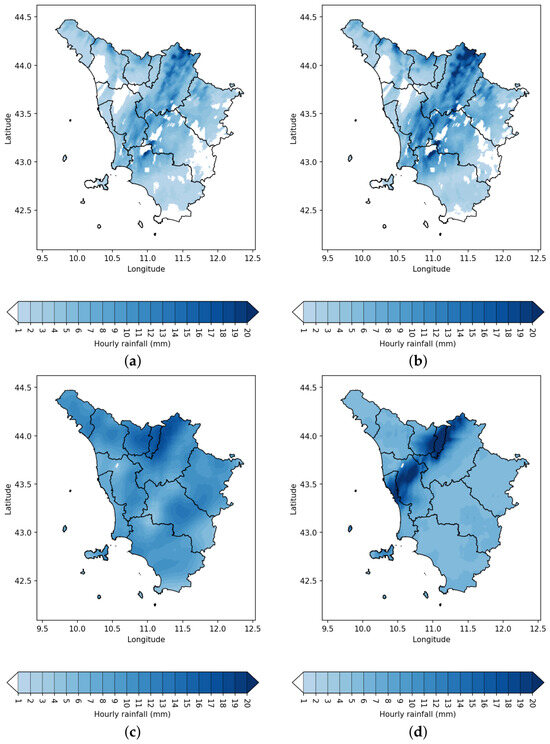
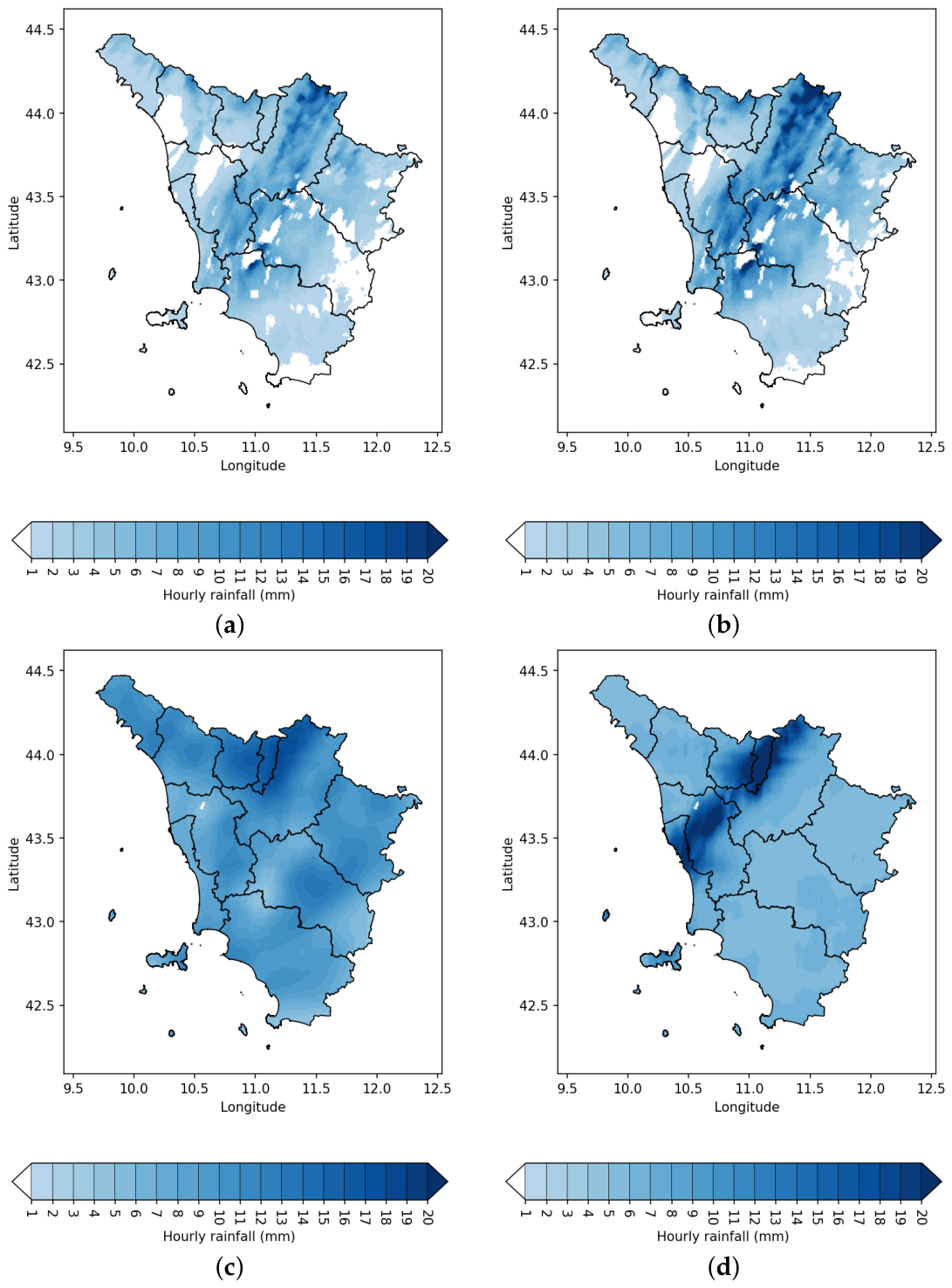
Figure 6 shows a qualitative example of the hourly rainfall maps produced from this volume, at the peak of the event, by the three estimation paradigms: a fixed $Z-R$ relation (Joss–Waldvogel), a data-driven $Z-R$ relation calibrated on the event (log-regression) and the deep models (the best baseline CNN and the reference U-Net). The two $Z-R$ models map the reflectivity core into rainfall through a pointwise power law, differing only in how strongly they scale it: The log-regression, fitted to compress reflectivity, yields a smoother dynamic range but still reproduces the field pixel by pixel. The deep models instead reorganize the field using the surrounding spatial context—U-Net produces a spatially more coherent estimate of the precipitation pattern than the baseline CNN.

Figure 6. Examples of hourly rainfall maps obtained from the radar volume of Figure 1 on 2 November 2023 at 21:00 UTC, comparing the following: (a) Joss–Waldvogel parametric $Z-R$ relationship; (b) adaptive $Z-R$ relationship calculated by means of log-regression on the rain gauges of the Pistoia province; (c) baseline CNN with wMSE optimization; (d) proposed U-Net with wMAE optimization. Parametric models use only 2000 m CAPPI layers, as shown in Figure 3, with hourly time slots and rainfalls. Nonparametric models use the eight CAPPI slices shown in Figure 1, with six time slots of 10^′ each and rain-gauge data resampled at 10^′.

It is noticeable that the four rainfall maps are quite different from each other. The two produced by the parametric methods are quite similar, whereas the two produced by the neural methods are substantially different from the first two, and also from each other. To get an idea of the reliability of the obtained values, quality measurements were performed between the maps and the rainfall data. In one case, these were extended to the entire region, and in another only to the provinces that were not used for training either by the log-regression or the networks, namely, the provinces of Pisa and Livorno. The results are shown in Table 3, where the two panels exhibit complementary behavior. The error statistics deteriorate for all methods over Pisa and Livorno, the provinces that experienced the heaviest rainfall. For a given relative discrepancy, larger rainfall amounts inevitably produce larger absolute errors; moreover, because all estimators tend to underestimate the most intense precipitation, the negative bias also increases. Correlation, however, reveals a different picture. Over the entire study region, the observations span a broad range of rainfall accumulations, and any monotonic function of reflectivity captures part of this large-scale variability, thereby sustaining the moderate correlations achieved by the parametric relations ($r\approx 0.24$). Restricting the evaluation to the two adjacent coastal provinces substantially reduces this dynamic range, leaving only the fine-scale variability within the convective system. Under these conditions, a pointwise power-law relationship between reflectivity and rainfall carries little predictive information, and both parametric estimators drop to $r=-0.054$, effectively indicating no correlation. By contrast, the deep learning models exploit the spatial context, the vertical structure of the reflectivity field, and its short-term temporal evolution rather than relying on a single radar pixel, allowing them to maintain a substantially higher correlation ($r=0.634$).

Table 3. Rainfall estimation performance of the maps in Figure 6 (2 November 2023, 21:00 UTC), computed on all gauges in Tuscany and on gauges of Pisa and Livorno provinces only. Best value per column in bold.

All Gauges	MAE (mm)	RMSE (mm)	B (mm)	r
Joss–Waldvogel	8.63	13.30	−7.63	0.239
Log-regression (Pistoia)	8.12	12.65	−5.88	0.241
Baseline wMSE	8.17	11.02	−1.17	0.197
U-Net wMAE	6.46	9.36	−2.51	0.609
Pisa and Livorno Gauges	MAE (mm)	RMSE (mm)	B (mm)	r
Joss–Waldvogel	12.94	18.59	−12.84	−0.054
Log-regression (Pistoia)	12.12	17.94	−11.52	−0.054
Baseline wMSE	9.21	14.85	−7.74	0.287
U-Net wMAE	8.06	11.70	−5.04	0.634

Parametric methods produce estimates that are practically uncorrelated with the measures taken at different locations. The networks, and in particular the proposed U-Net, provide good spatial prediction of values independent of the training measurements. It should be noted that bias is not a qualifying parameter because, being a systematic error, it can be corrected [32]. The important scores are the correlation and the MAE or RMSE. The latter are lower when evaluated across the entire region, but still competitive even across independent provinces. The correlation r takes into account the shape of the rainfall map and is the strength of proposed methods. By chance, it turns out to be higher when calculated across independent provinces than across the entire region. This fact indicates the good spatial predictive capacity of the proposed U-Net method.

4. Discussion

The results obtained on a unique severe convective rain event in Tuscany, Italy, indicate that CNNs, and particularly the proposed $(2+1)D$ U-Net, are a viable alternative to purely parametric $Z-R$ methods. Two findings deserve emphasis because they were obtained under a deliberately conservative evaluation protocol.

First, the evaluation was spatially blocked at the province level and protected by a 10.5 km anti-leakage buffer, so that no training gauge ever fell inside the input window of a test gauge. This is a much harder test than a random partition: the absolute errors are correspondingly larger, and the correlations lower, than those one would obtain by interpolating between neighboring gauges. It is precisely under these conditions that the value of the learning approach becomes clear. The fixed $Z-R$ relations, and even a data-driven $Z-R$ relation calibrated on the event by a logarithmic regression, remain weak ($r\approx 0.21$): hence, the weakness is intrinsic to the point-scale reflectivity–rainfall mapping and cannot be removed by a better choice of coefficients. The U-Net, in contrast, generalizes to unseen regions during training, which is the operationally relevant scenario, producing rainfall maps even in the absence of rain-gauge data, just by leveraging radar coverage.

The persistent underestimation of the heaviest hours, common to all estimators, is mitigated by weighting the loss with the target value. The weighted variants reduce the negative bias at every rainfall intensity; the U-Net trained with the weighted MAE offers the best compromise among correlation, squared error, and calibration, and it was adopted as the reference model.

The main limitations remain the amount of data and computation that CNNs require and the fact that the present evidence comes from a single event—that is, a very scarce dataset to train the model. Extending the analysis to multiple events and larger domains and assessing the transfer of a trained network to geographical regions uncovered by gauges are the natural next steps.

5. Conclusions

In this study, we propose a deep learning approach for quantitative precipitation estimation from weather-radar and rain-gauge data. The architecture features a U-Net backbone designed to cope with data scarcity, integrated with $(2+1)D$ convolutional blocks that capture the spatial and temporal evolution of volumetric radar acquisitions.

The proposed DL model was benchmarked with a baseline CNN, four fixed parametric $Z-R$ relations, and a data-driven $Z-R$ relation achieved by log-regression. Weather-radar and rain-gauge observations were collected during the severe convective event that struck Tuscany, Italy, on 2 November 2023. The complete training and evaluation pipeline runs in less than 20^′ per configuration on an Apple MacBook Pro (M3 Max). The proposed U-Net architecture achieved the best correlation, with the lowest RMSE and MAE, of all of the methods compared. The bias values were more than halved with respect to parametric methods operating in the same configuration, while correlation values more than doubled.

Target-weighted losses further reduce the underestimation of intense rainfall. Given its scalability, the model can easily be adapted to larger and more diverse datasets. Future developments will extend it to multiple events and assess its robustness and transfer to regions not covered by rain gauges.

A final issue concerns investigating possible benefits stemming from the introduction of non-separable multiscale analysis [49] in the DL process. The use of a preprocessing stage of the reflectivity maps, such as those used for synthetic-aperture radar (SAR) data [50], is worth attention. Without the $3\times 3$ average, the performance of all tasks is significantly poorer.

The ability to estimate rainfall from radar coverage alone, once the model has been trained, is directly relevant to the applications mentioned in Section 1. Hydrological and hydraulic models are driven by a distributed precipitation field, and their weakest link is usually the headwater portion of the catchment: mountainous and sparsely instrumented, yet hydrologically dominant, since the rainfall falling there governs the discharge downstream within a few hours. Gauge-based interpolation and gauge-adjustment techniques are least reliable precisely there, whereas radar coverage is generally available. A trained model can therefore supply the rainfall forcing over ungauged headwaters, at the update rate of the radar scan, for flash-flood detection, river-flood modeling, and water-balance computation. Two caveats apply: the estimates are hourly accumulations, whereas flash-flood applications typically call for a sub-hourly update; and all estimators, including the proposed one, still underestimate the most intense hours, even though the target-weighted losses mitigate this behavior and a systematic bias can be corrected a posteriori [32].

References

- Michaelides, S.; Levizzani, V.; Anagnostou, E.; Bauer, P.; Kasparis, T.; Lane, J. Precipitation: Measurement, remote sensing, climatology and modeling. Atmos. Res. 2009, 94, 512–533. [Google Scholar] [CrossRef]
- McKee, J.L.; Binns, A.D. A review of gauge–radar merging methods for quantitative precipitation estimation in hydrology. Can. Water Resour. J./Rev. Can. Des Ressour. Hydr. 2016, 41, 186–203. [Google Scholar] [CrossRef]
- Lanza, L.G.; Vuerich, E. The WMO field intercomparison of rain intensity gauges. Atmos. Res. 2009, 94, 534–543. [Google Scholar] [CrossRef]
- Ahrens, B. Distance in spatial interpolation of daily rain gauge data. Hydrol. Earth Syst. Sci. 2006, 10, 197–208. [Google Scholar] [CrossRef]
- Wackernagel, H. Multivariate Geostatistics: An Introduction with Applications, 3rd ed.; Springer: Heidelberg, Germany, 2003. [Google Scholar]
- Piazza, A.D.; Conti, F.L.; Noto, L.V.; Viola, F.; Loggia, G.L. Comparative analysis of different techniques for spatial interpolation of rainfall data to create a serially complete monthly time series of precipitation for Sicily, Italy. Int. J. Appl. Earth Obs. Geoinf. 2011, 13, 396–408. [Google Scholar] [CrossRef]
- Mair, A.; Fares, A. Comparison of rainfall interpolation methods in a mountainous region of a tropical island. J. Hydrol. Eng. 2011, 16, 371–383. [Google Scholar] [CrossRef]
- Doviak, R.J.; Zrnić, D.S. Doppler Radar and Weather Observations, 2nd ed.; Academic Press: San Diego, CA, USA, 1993. [Google Scholar]
- Villarini, G.; Krajewsky, W.F. Review of the different sources of uncertainty in single polarization radar-based estimates of rainfall. Surv. Geophys. 2010, 31, 107–129. [Google Scholar] [CrossRef]
- McRoberts, D.B.; Nielsen-Gammon, J.W. Detecting beam blockage in radar-based precipitation estimates. J. Atmos. Ocean. Tech. 2017, 34, 1407–1422. [Google Scholar] [CrossRef]
- Hubbert, J.C.; Meymaris, G.; Romatschke, U.; Ellis, S.; Dixon, M. A new paradigm for automated ground clutter removal: Global regression filtering. J. Atmos. Ocean. Technol. 2025, 42, 589–620. [Google Scholar] [CrossRef]
- Wilson, J.W.; Brandes, E.A. Radar measurement of rainfall—A summary. Bull. Am. Meteorol. Soc. 1979, 60, 1048–1060. [Google Scholar] [CrossRef]
- Chapon, B.; Delrieu, G.; Gosset, M.; Boudevillain, B. Variability of rain drop size distribution and its effect on the Z–R relationship: A case study for intense Mediterranean rainfall. Atmos. Res. 2008, 87, 52–65. [Google Scholar] [CrossRef]
- Smith, J.A.; Hui, E.; Steiner, M.; Baeck, M.L.; Krajewski, W.F.; Ntelekos, A.A. Variability of rainfall rate and raindrop size distributions in heavy rain. Water Resour. Res. 2009, 45, 1–12. [Google Scholar] [CrossRef]
- Atlas, D.; Ulbrich, C.W.; Meneghini, R. The multiparameter remote measurement of rainfall. Radio Sci. 1984, 19, 3–22. [Google Scholar] [CrossRef]
- Lee, G.W.; Zawadzki, I. Variability of drop size distributions: Time-scale dependence of the variability and its effects on rain estimation. J. Appl. Meteorol. 2005, 44, 241–255. [Google Scholar] [CrossRef]
- Marshall, J.; Hitschfeld, W.; Gunn, K. Advances in radar weather. Adv. Geophys. 1955, 2, 1–56. [Google Scholar] [CrossRef]
- Joss, J.; Waldvogel, A. A method to improve the accuracy of radar-measured amounts of precipitation. In Proceedings of the 14th Conference on Radar Meteorology, Tucson, AZ, USA, 17–20 November 1970; pp. 237–238. [Google Scholar]
- Zhang, J.; Howard, K.; Langston, C.; Kaney, B.; Qi, Y.; Tang, L.; Grams, H.; Wang, Y.; Cockcks, S.; Martinaitis, S.; et al. Multi-Radar Multi-Sensor (MRMS) quantitative precipitation estimation: Initial operating capabilities. Bull. Am. Meteorol. Soc. 2016, 97, 621–638. [Google Scholar] [CrossRef]
- Adirosi, E.; Roberto, N.; Montopoli, M.; Gorgucci, E.; Baldini, L. Influence of disdrometer type on weather radar algorithms from measured DSD: Application to Italian climatology. Atmosphere 2018, 9, 360. [Google Scholar] [CrossRef]
- Zhang, J.; Tang, L.; Cocks, S.; Zhang, P.; Ryzhkov, A.; Howard, K.; Langston, C.; Kaney, B. A dual-polarization radar synthetic QPE for operations. J. Hydrometeorol. 2020, 21, 2507–2521. [Google Scholar] [CrossRef]
- Bringi, V.N.; Chandrasekar, V. Polarimetric Doppler Weather Radar: Principles and Applications; Cambridge University Press: Cambridge, UK, 2001. [Google Scholar] [CrossRef]
- Zrnic, D.S.; Ryzhkov, A.V. Polarimetry for weather surveillance radars. Bull. Am. Meteorol. Soc. 1999, 80, 389–406. [Google Scholar] [CrossRef]
- Ryzhkov, A.; Zhang, P.; Bukovčić, P.; Zhang, J.; Cocks, S. Polarimetric radar quantitative precipitation estimation. Remote Sens. 2022, 14, 1695. [Google Scholar] [CrossRef]
- Vulpiani, G.; Montopoli, M.; Delli Passeri, L.; Gioia, A.G.; Giordano, P.; Marzano, F.S. On the use of dual-polarized C-band radar for operational rainfall retrieval in mountainous areas. J. Appl. Meteorol. Climatol. 2012, 51, 405–425. [Google Scholar] [CrossRef]
- Gu, J.Y.; Ryzhkov, A.; Zhang, P.; Neilley, P.; Knight, M.; Wolf, B.; Lee, D.I. Polarimetric attenuation correction in heavy rain at C band. J. Appl. Meteorol. Climatol. 2011, 50, 39–58. [Google Scholar] [CrossRef]
- Ochoa-Rodríguez, S.; Wang, L.P.; Willems, P.; Onof, C. A review of radar-rain gauge data merging methods and their potential for urban hydrological applications. Water Resour. Res. 2019, 55, 6356–6391. [Google Scholar] [CrossRef]
- Sinclair, S.; Pegram, G. Combining radar and rain gauge rainfall estimates using conditional merging. Atmos. Sci. Lett. 2005, 6, 19–22. [Google Scholar] [CrossRef]
- Le, X.H.; Koyama, N.; Kikuchi, K.; Yamanouchi, Y.; Fukaya, A.; Yamada, T. Evaluating geostatistical and statistical merging methods for radar–gauge rainfall integration: A multi-method comparative study. Remote Sens. 2025, 17, 2622. [Google Scholar] [CrossRef]
- Brandes, E.A. Optimizing rainfall estimates with the aid of radar. J. Appl. Meteorol. Climatol. 1975, 14, 1339–1345. [Google Scholar] [CrossRef] [PubMed]
- Cuccoli, F.; Facheris, L.; Antonini, A.; Melani, S.; Baldini, L. Weather radar and rain-gauge data fusion for quantitative precipitation estimation: Two case studies. IEEE Trans. Geosci. Remote Sens. 2020, 58, 6639–6649. [Google Scholar] [CrossRef]
- Biondi, A.; Facheris, L.; Argenti, F.; Cuccoli, F. Comparison of different quantitative precipitation estimation methods based on a severe rainfall event in Tuscany, Italy, November 2023. Remote Sens. 2024, 16, 3985. [Google Scholar] [CrossRef]
- Biondi, A.; Facheris, L.; Argenti, F.; Cuccoli, F.; Antonini, A.; Melani, S. Assessing quantitative precipitation estimation methods based on the fusion of weather radar and rain-gauge data. IEEE Geosci. Remote Sens. Lett. 2024, 21, 3508005. [Google Scholar] [CrossRef]
- Krajewski, W.F. Cokriging radar-rainfall and rain gauge data. J. Geophys. Res. 1987, 92, 9571–9580. [Google Scholar] [CrossRef]
- Todini, E. A Bayesian technique for conditioning radar precipitation estimates to rain-gauge measurements. Hydrol. Earth Syst. Sci. 2001, 5, 187–199. [Google Scholar] [CrossRef]
- Hinton, G.E.; Salakhutdinov, R.R. Reducing the dimensionality of data with neural networks. Science 2006, 313, 504–507. [Google Scholar] [CrossRef] [PubMed]
- Lecun, Y.; Bengio, Y.; Hinton, G. Deep learning. Nature 2015, 521, 436–444. [Google Scholar] [CrossRef] [PubMed]
- Chen, H.; Chandrasekar, V.; Cifelli, R.; Xie, P. A machine learning system for precipitation estimation using satellite and ground radar network observations. IEEE Trans. Geosci. Remote Sens. 2020, 58, 982–994. [Google Scholar] [CrossRef]
- Han, L.; Zhao, Y.; Chen, H.; Chandrasekar, V. Advancing radar nowcasting through deep transfer learning. IEEE Trans. Geosci. Remote Sens. 2022, 60, 4100609. [Google Scholar] [CrossRef]
- Chen, H.; Chandrasekar, V.; Tan, H.; Cifelli, R. Rainfall estimation from ground radar and TRMM precipitation radar using hybrid deep neural networks. Geophys. Res. Lett. 2019, 46, 10669–10678. [Google Scholar] [CrossRef]
- Moraux, A.; Dewitte, S.; Cornelis, B.; Munteanu, A. Deep learning for precipitation estimation from satellite and rain gauges measurements. Remote Sens. 2019, 11, 2463. [Google Scholar] [CrossRef]
- Osman, N.S.; Tahir, W. Machine learning-based model for enhanced quantitative precipitation estimates (QPE) from radar images extracted features. In Proceedings of the 2023 IEEE 8th International Conference on Recent Advances and Innovations in Engineering (ICRAIE), Kuala Lumpur, Malaysia, 2–3 December 2023; pp. 1–5. [Google Scholar] [CrossRef]
- Li, W.; Chen, H.; Han, L. Polarimetric radar quantitative precipitation estimation using deep convolutional neural networks. IEEE Trans. Geosci. Remote Sens. 2023, 61, 4102911. [Google Scholar] [CrossRef]
- Huangfu, J.; Hu, Z.; Zheng, J.; Wang, L.; Zhu, Y. Study on quantitative precipitation estimation by polarimetric radar using deep learning. Adv. Atmos. Sci. 2024, 41, 1147–1160. [Google Scholar] [CrossRef]
- Report Meteorologico: Evento 2 Novembre 2023. Technical Report (In Italian), Consorzio LaMMA (Environmental Modeling and Monitoring Laboratory for Sustainable Development). 2023. Available online: https://www.lamma.toscana.it/clima/report/eventi/evento_02112023.pdf (accessed on 10 June 2026).
- Aiazzi, B.; Alparone, L.; Baronti, S.; Pippi, I.; Selva, M. Generalised Laplacian pyramid-based fusion of MS+P image data with spectral distortion minimisation. In 2002 International Symposium of ISPRS Commission III on Photogrammetric Computer Vision, PCV 2002; ISPRS: Hannover, Germany, 2002; Volume 34, ISPRS Archives; pp. 3–6. [Google Scholar]
- Ronneberger, O.; Fischer, P.; Brox, T. U-net: Convolutional networks for biomedical image segmentation. In International Conference on Medical Image Computing and Computer-Assisted Intervention; Lecture Notes in Computer Science; Springer: Berlin/Heidelberg, Germany, 2015; pp. 234–241. [Google Scholar] [CrossRef]
- Tran, D.; Wang, H.; Torresani, L.; Ray, J.; Lecun, Y.; Paluri, M. A closer look at spatiotemporal convolutions for action recognition. In Proceedings of the IEEE Computer Society Conference on Computer Vision and Pattern Recognition, Salt Lake City, UT, USA, 18–23 June 2018; pp. 6450–6459. [Google Scholar] [CrossRef]
- Garzelli, A.; Nencini, F.; Alparone, L.; Baronti, S. Multiresolution fusion of multispectral and panchromatic images through the curvelet transform. In Proceedings of the 2005 IEEE International Geoscience and Remote Sensing Symposium, Seoul, Republic of Korea, 25–29 July 2005; pp. 2838–2841. [Google Scholar] [CrossRef]
- Lapini, A.; Bianchi, T.; Argenti, F.; Alparone, L. Blind speckle decorrelation for SAR image despeckling. IEEE Trans. Geosci. Remote Sens. 2014, 52, 1044–1058. [Google Scholar] [CrossRef]
Disclaimer/Publisher’s Note: The statements, opinions and data contained in all publications are solely those of the individual author(s) and contributor(s) and not of MDPI and/or the editor(s). MDPI and/or the editor(s) disclaim responsibility for any injury to people or property resulting from any ideas, methods, instructions or products referred to in the content. |
© 2026 by the authors. Licensee MDPI, Basel, Switzerland. This article is an open access article distributed under the terms and conditions of the Creative Commons Attribution (CC BY) license.