Abstract
Rare species at the edge of their range often persist after range contractions, yet basic information is typically lacking. We created species distribution models (SDMs) to guide field surveys for a disjunct population of Sessileflower Indian parsley (Cymopterus sessiliflorus; Apiaceae). We used historical observations to produce an initial model that guided field surveys in 2023. We refined the model using new observations from these surveys and the best predictors were shrubs, rock outcrops, mean monthly precipitation of the warmest quarter and rock type (area under the curve = 0.97). Suitable habitat (moderate-high and high classes) was predicted in <2% of Wyoming. We discovered 11 new populations over 2 summers. We collected 17 bee genera (n = 272 individuals) during C. sessiliflorus flowering suggesting diverse potential pollinators may transport pollen. Our model highlighted other areas predicted suitable and surveys in these areas may reveal new populations of this rare plant. The SDMs demonstrated how sparse historical data on rare species can be used to direct surveys in an efficient and effective manner. The information we gathered provided basic data for a rare plant at the periphery of its range where the most robust populations may occur making them critical for conservation efforts.
1. Introduction
An increasing number of studies demonstrate that whole plant communities are needed to function properly [1,2,3], yet information on rare plants are typically lacking. Data on rare plants are especially scarce, but studies are beginning to reveal that rare species often have critical roles in ecosystems and the functions they perform far outweigh their density [4,5,6]. Rare species are those that occur at low frequency or density on the landscape [7]. Such species have an increased risk of extinction due to their small ranges or sparse occurrences [4]. Basic information, critical to informing management decisions, is lacking for many rare species such as information about their phenology, life cycle, habitat associations and distribution. Rare species are typically of management concern because these species have a higher likelihood of being protected by state or federal agencies. Ensuring the persistence of populations requires an understanding of basic information which begins with their distribution on the landscape.
Studying a species at the edge of their range is critical, because these are the populations that persist after range contractions. Channell and Lomolino [8] measured how the geographic range of 245 species contracted and found that species did not persist at the heart of their ranges as was hypothesized, but instead remained at the peripheries of their distributions. The authors hypothesized that individuals at the edge of their range had higher genetic diversity due to local adaptation and, thus, were more capable of surviving adverse conditions. Disjunct populations of plants may live in different habitats and be pollinated by other species compared to individuals in the heart of their range. Therefore, populations at the edges of their range are excellent candidates for conservation and may be vital for species preservation because they are more likely to persist after a range contraction. The effects of range contraction depend on the dispersal of the species and the rate at which change occurs [9]. Range contractions usually occur due to stressors on populations such as changing land use, altered precipitation and thermal regimes, invasive species or diseases, phenological mismatch with pollinators, the decline of pollinators and others [10,11,12], as well as how species evolutionarily respond to these stressors [13]. Assessing threats and basic habitat needs of species is critical for both the species’ persistence and to inform our management to prevent range contractions and increased vulnerability.
Species distribution models (SDMs) are a useful tool to guide surveys that predict suitable habitat of a species and better define its distribution. These models predict the suitable habitat for a species using environmental (e.g., temperature, precipitation, etc.) and landscape (e.g., shrub cover, rock type, etc.) variables based on species presence data. SDMs have demonstrated accurate predictions when very few [14,15] to many observations are available, thus, this technique is applicable for a broad array of plants and animals, and is a commonly used method in the literature [16,17,18]. Species distribution models result in color-coded maps that show the probability of suitable habitat, making the assessment of areas that a species are most likely to inhabit more efficient. Species distribution models are especially useful when human resources, historical observations or funds to survey for rare species are limited.
The plant, Cymopterus sessiliflorus (Sessileflower Indian Parsley), is known from six locations in Wyoming, USA and we used species distribution models to guide surveys for new populations. Cymopterus sessiliflorus is a species of concern throughout its range in the Four Corners region of the southwestern USA (i.e., Colorado, Utah, New Mexico and Arizona) due to rarity, and a disjunct population occurs in central Wyoming. Few observations of C. sessiliflorus were known in Wyoming (13 specimens at six locations since 1983) resulting in little information to base management decisions upon [19]. The large spatial gap between known occurrences in the Four Corners region and central Wyoming highlights a lack of knowledge about the plant’s distribution. We hypothesized that (1) climate variables, particularly precipitation, would explain the most variance in the distribution of C. sessiliflorus given the species association with specific moisture regimes, (2) topographic and substrate features (e.g., proximity to rock outcrops) would improve model predictions beyond climate variables alone, and (3) field surveys would confirm the presence of C. sessiliflorus primarily in areas of moderate to high predicted habitat suitability. We used SDMs to guide walking surveys to search for new populations in Wyoming. Our surveys provide basic information about a rare species which expands knowledge about a critically imperiled species.
2. Materials and Methods
2.1. Study Species and Area
Cymopterus sessiliflorus (syn. Aletes sessiliflorus; Figure 1a) is a perennial forb with a branched woody base in the family Apiaceae and the subfamily Apioideae, which is endemic to western North America [20]. The first known collection of the plant was by H. Dwight, D. Ripley and Rupert C. Barneby in 1948 in New Mexico. William Theobald and Charles Tseng described this collection as the type for Aletes sessiliflorus [21]. In 2006, Ronald Hartman revised the genus to Cymopterus, based on characteristics of the fruit and leaves [22]. Cymopterus sessiliflorus was collected for the first time in Wyoming in 1983 by Erwin F. Evert and the plant has only been found in Fremont County since that time. Cymopterus sessiliflorus is found in three counties in southern Colorado (Montezuma, La Plata and Archuleta; [23]), three counties in southeastern Utah (San Juan, Garfield and Grand; [24]), four counties in New Mexico (McKinley, Rio Arriba, Sandoval and San Juan; [25]), and two counties in northeastern Arizona (Apache and Navajo; [24]).
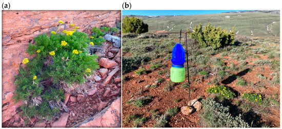
Figure 1.
(a) Cymopterus sessiflorus growing in central Wyoming in sandstone crevices. (b) Blue vane trap deployed near flowering C. sessiflorus plants to assess potential pollinators.
Cymopterus sessiliflorus typically grows in rocky outcroppings and crevices in pinyon-juniper woodland ranging from 1372 [26] to 2987 m elevation in the Four Corners region [27]. In Wyoming, the plant grows in the southeastern foothills of the Wind River Range which is composed of rock outcrops of Nugget Sandstone. This area of Wyoming receives an average of 33 cm of precipitation annually [28].
2.2. Species Distribution Modeling
We created maps predicting a suitable habitat for C. sessiflorus across Wyoming to direct surveys to find new populations. We made an initial map using maximum entropy models (Maxent; [29] with known presence points in Wyoming [30] to guide surveys during the first year of the project in 2023. We created a revised model by adding presence points discovered in 2023 to the pervious information. The revised map was used to guide surveys in 2024.
We considered 34 bioclimatic and landscape variables that were chosen a priori based on knowledge of the species and area [31,32,33,34] (Table 1). We summarized data from weather stations [35,36], vegetation variables derived from LANDFIRE [37], and other habitat and topographic variables (e.g., CTI, distance to rock outcrop) as potential predictors for explaining the occurrence of the species. Predictor values were extracted for presence (n = 6) and background (n = 10,000) locations in Program R (v4.3.2; University of Auckland, New Zealand) using the raster package [38,39]. Only one variable was retained when two or more variables were correlated (r ≥ 0.70). Variables were retained and identified as top predictors by maintaining higher area under the curve (AUC) values, differentiating between predicted probability of presence versus absence by assessing response curves, the percent contribution and permutation importance to the model, and variable importance results from a jackknife test. In cases where metrics for a predictor were conflicting (e.g., flat response curve but high percent contribution score), we assessed whether the SDM map appeared more refined (smaller area of the state highlighted as suitable habitat) and better aligned with the known biology of the plant (removing high elevation areas for a plant found in low elevations) to decide whether to keep the predictor as part of the final model. We used K-fold cross validation for all models, where k was equal to the total number of presence points. We tested all feature classes and we used regularization multiplier values of 1–3.

Table 1.
The variables used to predict suitable habitat in the initial and revised species distribution model for C. sessiliflorus, with their individual percent contribution and permutation importance.
We used historical locations from 1994, 2014 and 2019 where C. sessiliflorus was observed, and we generated random background points across Wyoming to guide 2023 surveys [40]. We modeled habitat suitability across the state because we wanted to minimize bias due to our small sample size and clustered points. Additionally, one of our goals is to provide information to look for this plant in other areas of Wyoming. Predictor variables (n = 32) were rasters with a resolution of 30 m2 with 1950–2000 BioClim variables from WorldClim [35] and LANDFIRE derived vegetation variables from ~2008. We added 13 additional presence points discovered from field surveys in 2023 to refine the model to guide surveys in 2024 (n = 19 total locations). Additionally, all BioClim variables were updated to the most recent data (2023) available from CHELSA [36] at ~1 km resolution (671 m × 924 m) which is a more appropriate resolution to use for modeling climatic data than downscaling to a finer resolution [41,42]. We resampled the resolution of all other variables to match that of BioClim’s to maintain the same resolution of all our data. While using fine scale predictors (<1 km) would be ideal for this plant to better capture microhabitat characteristics, all spatial data used for producing a SDM map must be at the same resolution and downscaling relevant climate data would result in providing inaccurate data to the model. Additionally, we added geologic rock type from USGS mineral resources as a potential predictor variable (n = 33) in the revised model based on field observations. Predicted suitable habitat (0–100%) was divided into quartiles (i.e., low, low-moderate, moderate-high, high) to predicted suitability.
2.3. Model Validation in the Field
We used the SDMs to guide field surveys to search for new populations of C. sessiliflorus. Surveys of C. sessiliflorus in central Wyoming were conducted between 16 May and 17 June 2023 and 22 May and 26 June 2024 when the species was flowering and fruiting by systematically searching for C. sessiliflorus by walking through areas. Survey routes were designed to assess areas with low to high predicted habitat suitability that were on accessible public land. We exhaustively searched each site by zigzagging throughout the area except in areas where the terrain was unsafe (e.g., steep slope). We recorded the number of C. sessiliflorus plants and we recorded their population boundaries in the field when new populations of C. sessiliflorus were discovered. Information on habitat, phenology, and plant associates were documented. We surveyed on public land in central Wyoming near Lander. Sixty points were selected for surveying and model-testing in 2023 using the initial model based on historical observations of C. sessiliflorus. The points selected for potential surveying in 2023 were equally divided among quartiles of predicted suitability with 15 surveys occurring within each quartile. Of the 60 potential survey locations, 33 were selected based on accessibility and time constraints, maintaining representation across the suitability categories. Survey locations in 2024 were selected using the revised SDM. Survey locations were selected based on accessibility, predicted habitat suitability, uniqueness from locations selected the previous year, and those areas not assessed in 2023.
2.4. Pollinating Insects
We collected pollinators to estimate which insects could visit this rare plant. We deployed 11 dry vane traps >50 m apart across three sites with flowering C. sessiliflorus populations for 24–48 h between 15 May and 1 June 2023 (Figure 1b; total deployment time of 515 h). We deployed a total of 12 vane traps across four sites with flowering plants for <70 h between 18 and 28 June in 2024 (818 h of deployment). We sampled later in 2024 to avoid catching bumble bee queens and to sample at a different time than in 2023 to collect a wider variety of bees. Traps were deployed for a variable amount of time due to weather and our ability to access the sites. We recorded the location, dates and times we deployed and retrieved traps, and the wind speed over the period. Upon collecting, insects were placed into a cooler and transferred to a freezer when we returned from the field. We sorted samples, identified each insect to order, and we pinned all the bees. We identified most bees to genus and we identified other bee taxa to species (e.g., Agapostemon, Bombus, Halictus) or subgenus (i.e., Lasioglossum) when keys were available [43,44].
3. Results
3.1. Habitat Suitability Based on Species Distribution Model
The initial map (Figure 2A) highlighted several areas that had a higher probability of suitable habitat for C. sessiliflorus. The top predictors for the initial C. sessiliflorus species distribution model were BioClim 18 (mean monthly precipitation of the warmest quarter), shrub index, and pinyon-juniper index with a linear feature class and a regularization multiplier of 2 (AUC = 0.996 ± 0.006; Supplementary Table S1). Of these variables, BioClim 18 provided the most informative data for the model because of this variable’s ability to differentiate between 0 and 100% probability of suitable habitat (Figure S1), the percent contribution to the model and its permutation importance (Table 1). Shrub index was moderately explanatory (Figure S2) followed by pinyon-juniper index (Supplementary Figure S3; Table 1). According to this model, 95% of the area in Wyoming (240,000 km2) was predicted to have a low probability of habitat suitability. Conversely, 8200 km2 (3%) was predicted to have low–moderate habitat suitability, 2600 km2 (1%) were predicted to have moderate to high habitat suitability and 2700 km2 (1%) was predicted to have high habitat suitability.
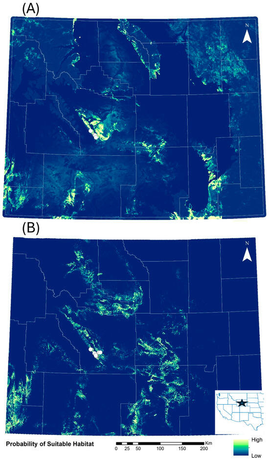
Figure 2.
(A) Predictive habitat suitability for Cymopterus sessiliforus across Wyoming, USA in the initial model that only used historical observations (n = 6, white circles). (B) Predictive habitat suitability in the revised model that used historical observations and those discovered in field surveys in 2023 (n = 19, white circles). Areas highlighted in yellow and light green have the highest predicted habitat suitability and areas in dark green or blue have the lowest. White lines show county boundaries within the state. The inset map shows the location of Wyoming in the western USA denoted by a star.
The revised model that included new populations discovered in 2023 highlighted a smaller area of the state as highly suitable habitat for C. sessiliflorus (Figure 2B). The top predictors for the revised model were shrub index, distance to the nearest rock outcrop, BioClim 18, rock type with linear and quadratic feature classes, and a regularization multiplier of 1 (AUC = 0.972 ± 0.028). Suitable habitat was most affected by the shrub index, followed by distance to rock outcrop, BioClim 18, and rock type in order of decreasing importance (Supplementary Figures S4–S7; Table 1 and Supplementary Table S2). This revised model more accurately reflected the range of elevations the plant has been found at previously compared to the initial model. Cymopterus sessiliflorus was found within BioClim 18 values of 67–108 mm, with a shrub index between 0.19 and 0.32, and <251 m from the nearest rocky outcrop. This plant was found in the sandstone (n = 12), mudstone (n = 5), fine-grained mixed clastic (n = 1), and alluvium (n = 1) rock types. The revised model predicted that 242,000 km2 of Wyoming (96%) was predicted as low habitat suitability, 5650 km2 (2%) was predicted as low–moderate habitat suitability, 3100 km2 (1%) was predicted to have moderate–high habitat suitability and 2500 km2 (<1%) of the state was predicted to have high habitat suitability for this plant.
3.2. Observations from Field Surveys
We conducted 33 surveys in 2023 (4 in low, 5 in low–moderate, 7 in moderate–high and 15 in high predicted habitat suitability areas) and 17 surveys in 2024 (1 in low, 5 in low–moderate, 6 in moderate–high, and 5 high habitat suitability; Supplementary Figure S8). We collected four specimens during the 2023 surveys which were submitted to the Rocky Mountain Herbarium, University of Wyoming. We walked an average of 4.2 km (range = 0.94–9.05 km) and 96 min (18 min–5.5 h) per survey during which we search systematically for C. sessiliflorus plants. Survey distance and time varied depending on the site of the predicted area and difficulty of the terrain. Cymopterus sessiliflorus was found during ten surveys in 2023 and one survey in 2024. Places where C. sessiliflorus were growing were within areas predicted as moderately high or highly suitable habitat according to the revised model.
Within each area where we discovered C. sessiiflorus, we found the species at multiple locations. We recorded 235 locations of C. sessiliflorus in 2023 (Figure 3). Of these, we mapped 194 locations across ~6 km2 of the Red Canyon with >2370 plants, 23 locations with >399 plants across ~60 km2 in the southeast part of Johnny Behind the Rocks and 18 locations with >370 plants near the intersection of Twin Creek Rd and US 287. We documented 25 locations across a ~20 km2 area with 2 to 35 plants per area in 2024 (241 plants total; Figure 3). The exact number of plants was not possible to count due to the large area, steep terrain and their growth form which made separating individuals difficult. Areas with C. sessiliflorus were usually in sagebrush steppe, grassland with junipers and other Apiaceae species. Chrysothamnus (rabbitbrush), Euphorbia (leafy spurge), Machaeranthera (tansyaster), Castilleja linariifolia (Wyoming Indian paintbrush), Sedum (stonecrop), Antennaria (pussytoes), Penstemon (beardtongue), and other asters were also commonly found among C. sessiliflorus in these locations.
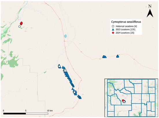
Figure 3.
Mapped locations of Cymopterus sessiliflorus in Fremont County, Wyoming. Historical observations are shown as white circles, 2023 observations are shown as blue triangles and 2024 observations are shown as red diamonds. The inset map shows the counties in Wyoming with the plant locations marked.
3.3. Potential Pollinators
We collected arthropods (n = 485) from 7 orders including five families and 17 genera of bees (Supplementary Table S3), which were active when C. sessiliflorus were flowering and thus potential pollinators. Most insects collected were bees (n = 272; 52%). Coleoptera (n = 167; 32%), other Hymenoptera (n = 28; 5%), Lepidoptera (n = 18; 3%), Hemiptera (n = 14; 2%), Diptera (n = 11; 2%), Orthoptera (n = 2; 0.3%), and Aranea (n = 1; 0.1%) were collected at lower abundances. Agapostemon was the most abundant genera collected in 2023 and Bombus was the most abundant genus collected in 2024 (Figure 4A). Andrena and Habropoda were only collected in 2023, and Anthidium, Ashmeadiella, Ceratina, Colletes, Diadasia and Melissodes were only collected in 2024 (Supplementary Table S4). Seven species of Bombus were caught over both seasons (Figure 4B). Bombus huntii was most abundant in 2023 and B. nevadensis was the most abundant in 2024. The wind speed ranged from 0 to 2.8 m/s during trap deployment.
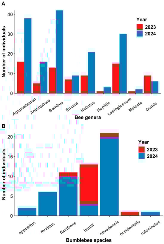
Figure 4.
(A) The number of bees in each genus collected between years in traps placed near flowering Cymopterus sessiliflorus plants. (B) The number of each bumblebee (Bombus) species caught in traps. Bumblebees were more abundant in 2024 compared to 2023, and Bombus nevadensis, B. huntii and B. flavifrons were the most common.
4. Discussion
The species distribution models we created guided field surveys enabling us to discover 11 new populations of C. sessiliflorus in central Wyoming. Modeling habitat suitability is a valuable method to direct field surveys as was demonstrated by most new populations occurring in moderately high and highly predicted suitable habitat [45]. Maxent models perform well even when few confirmed presence points are known as is common for rare species [46,47]. Species distribution models were used to direct surveys for a rare beetle, Hygrotus diversipes, and helped discover new sites [48]. Maxent was also one of the best performing models that guided surveys for rare plants in California, which lead to the discovery of new species occurrences [49]. We suggest using SDMs to focus field surveys because models can direct efforts across a large landscape which saves funds and precious field time. Refining our model with new information was critical, likely due to the increased sample size (from 6 to 19 presence points), the addition of rock type as a predictor, and the updated climate data, all of which improved predictions.
Validating our model by surveying in each class of habitat suitability was critical to produce a higher quality final product that more accurately predicted suitability. Dividing modeled habitat suitability into categories and surveying within each class was critical to refine the model and ensure our sampling scheme was balanced. Surveying all classes was critical to validate the model. We validated the model in central Wyoming; however, the model predicted suitable habitat for C. sessiliflorus in other parts of the state and we recommend surveying there. Surveys in these areas could reveal that C. sessiliflorus is more widely distributed; however, SDMs commonly overpredict suitable habitat, as models identify areas with appropriate environmental conditions but cannot account for dispersal limitation, biotic interactions, or historical factors that may predict species occurrence. Therefore, while our model prediction suggests additional areas warrant surveying, we do not interpret all predicted suitable habitat as part of the species range [50,51]. Distance to rock outcrop and rock type were top predictors for the final C. sessiliflorus model and should be considered if more surveys are undertaken because of the tight correlation between them and the occurrence of the plant. Knowing the abundance and distribution of rare species is critical to manage rare plants, and knowing the distribution of a rare species is the first step in acquiring basic information about the species. The combination of on-the-ground surveys with informed SDMs provided data that future work can springboard from [52,53]. The combination of SDM predictions with ground-truthing surveys provides immediate conservation value through discovering new populations and longer-term value through improved understanding of habitat requirements.
The decline of species is of upmost concern as some plants and animals are declining, which has the potential to alter ecosystem processes [5,6]. Most species who underwent range contractions tended to persist in peripheral populations, making information critical. In our study, future range shifts or contractions may center around the Wyoming populations of C. sessiliflorus, because they are on the “cool edge” (i.e., the poleward side) of the species’ known range [54], making them particularly important to conserve [55]. Cymopterus sessiliflorus may have different relationships with the surrounding plant community compared to the Four Corners populations due to the large distance between them and different habitats. The pattern in which range contractions occur likely vary depending on the environmental changes and species-specific characteristics making each species response unique. Plants are of particular concern because of expectations that many species will “lag” behind rapid changes in abiotic conditions [56]. Furthermore, species are not only limited by the amount of suitable habitat available, but whether they can successfully access and colonize that habitat [57].
Our surveys revealed a diversity of bees that could potentially pollinate C. sessiliflorus and provides baseline data for future comparisons. Wyoming is home to a rich community of pollinators as the state has western and eastern distributed species, and also been found in nearby collections [58]. In fact, Wyoming has the highest species richness of bumble bees in the US [59] at 26 species [60]. Pollinator traps were deployed later in the season in 2024 than in 2023, which may have contributed to differences in the taxa collected. These differences also demonstrated how the insects that pollinate C. sessiliflorus can change depending on phenology among years and locations. In the future, earlier trapping, target netting and video recording of insects on C. sessiliflorus, as well as analysis of pollen samples collected from specimens, would provide more detailed information on which species are transporting the pollen of this plant. Cymopterus species are capable of self-pollination, but the degree to which C. sessiliflorus does so is unknown. Seed-set experiments that identify pollen limitation can offer insights into the management needs of this species at the periphery of their range. Bombus occidentalis was observed near C. sessiliflorus, which is a bumble bee that has suffered drastic declines in their abundance [61]. The association between a rare plant and a declining bumble bee provides a possible glimpse into future monitoring and management, despite only a single observation.
Flowering plants and pollinators are critically linked by pollinators distributing pollen among individual plants and flowers providing food for pollinators. We collected information on pollinators to provide baseline information on the bees that were active during the flowering period and who could potentially transport pollen. We did not assess which species pollinated C. sessiliforus due to limited funds; however, such information could be measured in the future using the specimens deposited at the Center for Invertebrate Studies, University of Wyoming. Information about the insects that pollinate rare plants contributes information about the challenges a species faces. For example, rare plants pollinated by common, generalist pollinators tend to have more stable populations than rare plants pollinated by rare or specialist species [55]. The pollination networks describing the interactions of C. sessiliflorus with insects likely differ between the Four Corners region and the disjunct populations in Wyoming predicting that region-specific information is critical. Therefore, understanding the unique ecology of rare plants at the edge of their range is crucial to conserving and managing populations and communities, and protecting genetic diversity under future climate scenarios [8,55,62].
5. Conclusions
Species ranges can shift or contract due to anthropogenic and climactic stressors leading to novel management problems. We lack baseline data describing the distribution and habitat requirements for many species, with especially rare ones exacerbating the dilemma. Having basic information provides insight into how species are affected by changing temperature and precipitation regimes among other challenges. Basic baseline data allows us to compare the distribution and habitat requirements of a species over time; however, the lack of data limits the potential for management actions. Species distribution models are one tool that allows us to bolster information about rare species even when few observations are available. Our study demonstrated how limited information can be used to increase knowledge about a rare plant, including distribution, habitat requirements and phenology. Species distribution models have also been used to assess changes in predicted suitable habitat between the periods by creating separate SDMs using historical and current observations [63]. We demonstrated how SDMs can be leveraged to efficiently generate new information with limited funds or data, and our methods can be used for plant or animal species. Species distribution models can provide a springboard for future investigations into the habitat needs of rare species such as C. sessiliflorus, their dispersal abilities, and how they interact with the surrounding community.
Supplementary Materials
The following supporting information can be downloaded at: https://www.mdpi.com/article/10.3390/environments13010032/s1, Figure S1: The response curve of BioClim 18 in the final model for C. sessiliflorus historic locations (n = 6). The cloglog transformation of probability of presence (0–1.0) is on the y-axis with BioClim 18 values (mm of mean monthly precipitation of the warmest quarter) on the x-axis. The red line represents the mean response of BioClim 18 across six replicate Maxent runs, with the ± 1 standard deviation in blue; Figure S2: The response curve of Shrub Index in the final model for C. sessiliflorus historic locations (n = 6). The cloglog transformation of probability of presence (0–1.0) is on the y-axis with Shrub Index values on the x-axis. The red line represents the mean response of Shrub Index across six replicate Maxent runs, with the ± 1 standard deviation in blue; Figure S3: The response curve of Pinyon-Juniper Index in the final model for C. sessiliflorus historic locations (n = 6). The cloglog transformation of probability of presence (0.4–1.0) is on the y-axis with Pinyon-Juniper Index values on the x-axis. The red line represents the mean response of Pinyon-Juniper Index across six replicate Maxent runs, with the ± 1 standard deviation in blue; Figure S4: The response curve of Shrub Index in the final model for C. sessiliflorus historic and 2023 locations (n = 19). The cloglog transformation of probability of presence (0–1.0) is on the y-axis with Shrub Index values on the x-axis. The red line represents the mean response of Shrub Index across 19 replicate Maxent runs, with the ± 1 standard deviation in blue; Figure S5: The response curve of Distance to the nearest rock outcrop in the final model for C. sessiliflorus historic and 2023 locations (n = 19). The cloglog transformation of probability of presence (0-0.9) is on the y-axis with Distances to the nearest rock outcrop on the x-axis. The red line represents the mean response of Distance to the nearest rock outcrop across 19 replicate Maxent runs, with the ± 1 standard deviation in blue; Figure S6: The response curve of BioClim 18 in the final model for C. sessiliflorus historic and 2023 locations (n = 19). The cloglog transformation of probability of presence (0–0.9) is on the y-axis with BioClim 18 values (mm of mean monthly precipitation of the warmest quarter) on the x-axis. The red line represents the mean response of BioClim 18 across 19 replicate Maxent runs, with the ± 1 standard deviation in blue; Figure S7: The response curve of Geology rock type in the final model for C. sessiliflorus historic and 2023 locations (n = 19). The cloglog transformation of probability of presence (0.6–0.9) is on the y-axis with Geology Rocktype categories on the x-axis. The red line represents the mean response of Geology Rocktype across 19 replicate Maxent runs, with the ± 1 standard deviation in blue; Figure S8: The tracks recorded for all Cymopterus sessiliflorus surveys conducted in 2023 (blue) and 2024 (red). The inset map shows the counties of Wyoming with the tracks represented in southern Fremont County; Table S1: All predictors considered for inclusion in Maxent models for making species distribution maps of C. sessiliflorus, with a definition of each variable and where the data was acquired or what data was used to derive the variable. Top variables included in either final model are shaded in light gray; Table S2: All categories of geology rock types in Wyoming as classified by USGS Mineral Resources, with each category’s assigned numeric code used for modeling; Table S3: Bees identified from locations where C. sessiliflorus were blooming, the number of individuals caught, and the percentage of total bees they represent. Table S4: The number of genera caught in pollinator traps in 2023 and 2024. Shaded rows indicate that that genus was only caught during one year.
Author Contributions
Conceptualization, J.H. and L.M.T.; methodology, J.H. and L.M.T.; validation, K.A.C.; formal analysis, M.L.W., B.P.T. and K.A.C.; investigation, J.H., B.P.T. and M.L.W.; resources, L.M.T.; writing—original draft preparation, M.L.W., J.H. and L.M.T.; writing—review and editing, M.L.W., K.A.C., J.H. and L.M.T.; visualization, M.L.W. and K.A.C.; supervision, L.M.T.; project administration, L.M.T. funding acquisition, J.H. and L.M.T. All authors have read and agreed to the published version of the manuscript.
Funding
This research was funded by the US Bureau of Land Management, Lander Field Office (L22AC00232).
Data Availability Statement
Data is available from the Wyoming Natural Diversity Database at https://www.uwyo.edu/wyndd/index.html (accessed on 1 October 2025).
Acknowledgments
Emma Freeland provided logistical help that was critical for conducting surveys. Rachel Russel and Teresa Tibbets helped collect vane traps.
Conflicts of Interest
The authors declare no conflicts of interest.
References
- Gibson, R.H.; Nelson, I.L.; Hopkins, G.W.; Hamlett, B.J.; Memmott, J. Pollinator webs, plant communities and the conservation of rare plants: Arable weeds as a case study. J. Appl. Ecol. 2006, 43, 246–257. [Google Scholar] [CrossRef]
- Carvalheiro, L.; Barbosa, E.; Memmott, J. Pollinator networks, alien species and the conservation of rare plants: Trinia glauca as a case study. J. Appl. Ecol. 2008, 45, 1419–1427. [Google Scholar] [CrossRef]
- Wei, N.; Kaczorowski, R.L.; Arceo-Gómez, G.; O’Neill, E.M.; Hayes, R.A.; Ashman, T.L. Pollinators contribute to the maintenance of flowering plant diversity. Nature 2021, 597, 688–692. [Google Scholar] [CrossRef]
- Flather, C.; Sieg, C. Species Rarity: Definition, Causes, and Classification; Island Press: Washington, DC, USA, 2007; pp. 40–66. [Google Scholar]
- Dee, L.E.; Cowles, J.; Isbell, F.; Pau, S.; Gaines, S.D.; Reich, P.B. When Do Ecosystem Services Depend on Rare Species? Trends Ecol. Evol. 2019, 34, 746–758. [Google Scholar] [CrossRef]
- Jain, M.; Flynn, D.F.B.; Prager, C.M.; Hart, G.M.; DeVan, C.M.; Ahrestani, F.S.; Palmer, M.I.; Bunker, D.E.; Knops, J.M.H.; Jouseau, C.F.; et al. The importance of rare species: A trait-based assessment of rare species contributions to functional diversity and possible ecosystem function in tall-grass prairies. Ecol. Evol. 2014, 4, 104–112. [Google Scholar] [CrossRef]
- Lyons, K.; Brigham, C.; Traut, B.; Schwartz, M. Rare Species and Ecosystem Functioning. Conserv. Biol. 2005, 19, 1019–1024. [Google Scholar] [CrossRef]
- Channell, R.; Lomolino, M.V. Trajectories to extinction: Spatial dynamics of the contraction of geographical ranges. J. Biogeogr. 2000, 27, 169–179. [Google Scholar] [CrossRef]
- Arenas, M.; Ray, N.; Currat, M.; Excoffier, L. Consequences of range contractions and range shifts on molecular diversity. Mol. Biol. Evol. 2012, 29, 207–218. [Google Scholar] [CrossRef]
- Rogan, J.E.; Parker, M.R.; Hancock, Z.B.; Earl, A.D.; Buchholtz, E.K.; Chyn, K.; Martina, J.; Fitzgerald, L.A. Genetic and demographic consequences of range contraction patterns during biological annihilation. Sci. Rep. 2023, 13, 1691. [Google Scholar] [CrossRef] [PubMed]
- Parmesan, C.; Gaines, S.; Gonzalez, L.; Kaufman, D.M.; Kingsolver, J.; Townsend Peterson, A.; Sagarin, R. Empirical perspectives on species borders: From traditional biogeography to global change. Oikos 2005, 108, 58–75. [Google Scholar] [CrossRef]
- Faurby, S.; Araújo, M.B. Anthropogenic range contractions bias species climate change forecasts. Nat. Clim. Change 2018, 8, 252–256. [Google Scholar] [CrossRef]
- Diamond, S.E. Contemporary climate-driven range shifts: Putting evolution back on the table. Funct. Ecol. 2018, 32, 1652–1665. [Google Scholar] [CrossRef]
- Pearson, R.G. Species’ Distribution Modeling for Conservation Educators and Practitioners; Center for Biodiversity and Conservation, American Museum of Natural History: New York, NY, USA, 2010. [Google Scholar]
- Proosdij, A.S.J.; Sosef, M.; Wieringa, J.; Raes, N. Minimum required number of specimen records to develop accurate species distribution models. Ecography 2016, 39, 542–552. [Google Scholar] [CrossRef]
- McCune, J. Species distribution models predict rare species occurrences despite significant effects of landscape context. J. Appl. Ecol. 2016, 53, 1871–1879. [Google Scholar] [CrossRef]
- Rhoden, C.M.; Peterman, W.E.; Taylor, C.A. Maxent-directed field surveys identify new populations of narrowly endemic habitat specialists. PeerJ 2017, 5, e3632. [Google Scholar] [CrossRef]
- Ahmadi, K.; Mahmoodi, S.; Pal, S.C.; Saha, A.; Chowdhuri, I.; Nguyen, T.T.; Jarvie, S.; Szostak, M.; Socha, J.; Thai, V.N. Improving species distribution models for dominant trees in climate data-poor forests using high-resolution remote sensing. Ecol. Model. 2023, 475, 110190. [Google Scholar] [CrossRef]
- Rocky MountainHerbarium. Occurance dataset. Available online: https://www.rockymountainherbarium.org/ (accessed on 15 February 2023).
- Downie, S.R.; Hartman, R.L.; Sun, F.-J.; Katz-Downie, D.S. Polyphyly of the spring-parsleys (Cymopterus): Molecular and morphological evidence suggests complex relationships among the perennial endemic genera of western North American Apiaceae. Can. J. Bot. 2002, 80, 1295–1324. [Google Scholar] [CrossRef]
- Theobald, W.L.; Tseng, C.C.; Mathias, M.E. A Revision of Aletes and Neoparrya (Umbelliferae). Brittonia 1963, 16, 296–315. [Google Scholar] [CrossRef]
- Hartman, R.L. New combinations in the genus Cymopterus (Apiaceae) of the southwestern United States. SIDA Contrib. Bot. 2006, 22, 955–957. [Google Scholar]
- Fertig, W. Flora of Colorado. 2015. Jennifer Ackerfield. Syst. Bot. 2016, 40, 1159–1160. [Google Scholar] [CrossRef]
- Intermountain Region Herbaria Network. Available online: https://intermountainbiota.org/portal (accessed on 6 June 2023).
- Allred, K.W.; Ivey, R.D.; Jercinovic, E.M. Flora Neomexicana; Kelly, W.A., Ed.; BRIT Press: Fort Worth, TX, USA, 2008. [Google Scholar]
- California Botanic Garden Herbarium. Occurrence Dataset. Available online: https://www.calbg.org/collections/herbarium (accessed on 6 June 2023).
- San Juan College Herbarium. Occurrence Dataset. Available online: https://portal.idigbio.org/portal/recordsets/8ec76c75-a673-4682-bfde-00a18bc12794 (accessed on 6 June 2023).
- Western Regional Climate Center. 2025. Available online: https://wrcc.dri.edu/ (accessed on 15 December 2023).
- Steven, J.; Phillips, M.D.; Schapire, R.E. Maxent Software for Modeling Species Niches and Distributions (Version 3.4.1). Available online: http://biodiversityinformatics.amnh.org/open_source/maxent/ (accessed on 15 March 2023).
- Phillips, S.J.; Anderson, R.P.; Schapire, R.E. Maximum entropy modeling of species geographic distributions. Ecol. Model. 2006, 190, 231–259. [Google Scholar] [CrossRef]
- Davidson, A.; Aycrigg, J.; Grossmann, E.; Kagan, J.; Lennartz, S.; McDonough, S.; Miewald, T.; Ohmann, J.; Radel, A.; Sajwaj, T. Digital Land Cover Map for the Northwestern United States: Northwest Gap Analysis Project; USGS GAP Analysis Program: Moscow, ID, USA, 2009.
- Gesch, D.; Oimoen, M.; Greenlee, S.; Nelson, C.; Steuck, M.; Tyler, D. The national elevation dataset. Photogramm. Eng. Remote Sens. 2002, 68, 5–32. [Google Scholar]
- Jenness, J. Topographic Position Index (tpi_jen. avx_extension for Arcview 3. x, v. 1.3 a, Jenness Enterprises [EB/OL]. 2006. Available online: http://www.jennessent.com/arcview/tpi.htm (accessed on 10 March 2023).
- Stillman, S.T. A comparison of Three Automated Precipitation Simulation Models: ANUSPLIN, MTCLIM-3D, and PRISM. Master’s Thesis, Montana State University, Bozeman, MT, USA, 1996. [Google Scholar]
- Hijmans, R.J.; Cameron, S.E.; Parra, J.L.; Jones, P.G.; Jarvis, A. Very high resolution interpolated climate surfaces for global land areas. Int. J. Climatol. A J. R. Meteorol. Soc. 2005, 25, 1965–1978. [Google Scholar] [CrossRef]
- Karger, D.N.; Conrad, O.; Böhner, J.; Kawohl, T.; Kreft, H.; Soria-Auza, R.W.; Zimmermann, N.E.; Linder, H.P.; Kessler, M. Climatologies at high resolution for the earth’s land surface areas. Sci. Data 2017, 4, 170122. [Google Scholar] [CrossRef]
- LANDFIRE. Existing Vegetation Type Layer, LANDFIRE 1.1.0. Available online: https://www.landfire.gov/viewer/ (accessed on 9 February 2024).
- Hijmans, R.J. Raster: Geographic Data Analysis and Modeling. 2023. Available online: https://cran.r-project.org/web/packages/raster/index.html (accessed on 1 October 2025).
- R Core Team. R: A Language and Environment for Statistical Computing, 4.2.2; R Foundation for Statistical Computing: Vienna, Austria, 2022. [Google Scholar]
- Barbet-Massin, M.; Jiguet, F.; Albert, C.H.; Thuiller, W. Selecting pseudo-absences for species distribution models: How, where and how many? Methods Ecol. Evol. 2012, 3, 327–338. [Google Scholar] [CrossRef]
- Lanzante, J.R.; Dixon, K.W.; Nath, M.J.; Whitlock, C.E.; Adams-Smith, D. Some pitfalls in statistical downscaling of future climate. Bull. Am. Meteorol. Soc. 2018, 99, 791–803. [Google Scholar] [CrossRef]
- Pourmokhtarian, A.; Driscoll, C.T.; Campbell, J.L.; Hayhoe, K.; Stoner, A.M. The effects of climate downscaling technique and observational data set on modeled ecological responses. Ecol. Appl. 2016, 26, 1321–1337. [Google Scholar] [CrossRef]
- Tronstad, L.; Dillon, M. Field Guide to Wyoming’s Native Bees; Biodiversity Institute, University of Wyoming: Laramie, WY, USA, 2019. [Google Scholar]
- Williams, P.H.; Thorp, R.W.; Richardson, L.L.; Colla, S.R. Bumble bees of north America. In Bumble Bees of North America; Princeton University Press: Princeton, NJ, USA, 2014. [Google Scholar]
- Miller, J. Species distribution modeling. Geogr. Compass 2010, 4, 490–509. [Google Scholar] [CrossRef]
- Elith, J.; Graham, C.H.; Anderson, R.P.; Dudík, M.; Ferrier, S.; Guisan, A.; Hijmans, R.J.; Huettmann, F.; Leathwick, J.R.; Lehmann, A. Novel methods improve prediction of species’ distributions from occurrence data. Ecography 2006, 29, 129–151. [Google Scholar] [CrossRef]
- Abdelaal, M.; Fois, M.; Fenu, G.; Bacchetta, G. Using MaxEnt modeling to predict the potential distribution of the endemic plant Rosa arabica Crép. in Egypt. Ecol. Inform. 2019, 50, 68–75. [Google Scholar] [CrossRef]
- Tronstad, L.M.; Brown, K.M.; Andersen, M.D. Using species distribution models to guide field surveys for an apparently rare aquatic beetle. J. Fish Wildl. Manag. 2018, 9, 330–339. [Google Scholar] [CrossRef]
- Williams, J.N.; Seo, C.; Thorne, J.; Nelson, J.K.; Erwin, S.; O’Brien, J.M.; Schwartz, M.W. Using species distribution models to predict new occurrences for rare plants. Divers. Distrib. 2009, 15, 565–576. [Google Scholar] [CrossRef]
- Marcer, A. A Contribution to the Use, Modelling and Organization of Data in Biodiversity Conservation; Universitat Autònoma de Barcelona: Barcelona, Spain, 2013. [Google Scholar]
- Amirkhiz, R.G.; Frey, J.K.; Cain, J.W., III; Breck, S.W.; Bergman, D.L. Predicting spatial factors associated with cattle depredations by the Mexican wolf (Canis lupus baileyi) with recommendations for depredation risk modeling. Biol. Conserv. 2018, 224, 327–335. [Google Scholar] [CrossRef]
- Rodríguez, J.P.; Brotons, L.; Bustamante, J.; Seoane, J. The application of predictive modelling of species distribution to biodiversity conservation. Divers. Distrib. 2007, 13, 243–251. [Google Scholar] [CrossRef]
- Crawford, P.H.; Hoagland, B.W. Using species distribution models to guide conservation at the state level: The endangered American burying beetle (Nicrophorus americanus) in Oklahoma. J. Insect Conserv. 2010, 14, 511–521. [Google Scholar] [CrossRef]
- Chen, I.-C.; Hill, J.K.; Ohlemüller, R.; Roy, D.B.; Thomas, C.D. Rapid Range Shifts of Species Associated with High Levels of Climate Warming. Science 2011, 333, 1024–1026. [Google Scholar] [CrossRef] [PubMed]
- Rehm, E.; Olivas, P.; Stroud, J.; Feeley, K. Losing your edge: Climate change and the conservation value of range-edge populations. Ecol. Evol. 2015, 5, 4315–4326. [Google Scholar] [CrossRef]
- McNichol, B.H.; Russo, S.E. Plant Species’ Capacity for Range Shifts at the Habitat and Geographic Scales: A Trade-Off-Based Framework. Plants 2023, 12, 1248. [Google Scholar] [CrossRef]
- Brodie, J.F.; Freeman, B.G.; Mannion, P.D.; Hargreaves, A.L. Shifting, expanding, or contracting? Range movement consequences for biodiversity. Trends Ecol. Evol. 2025, 40, 439–448. [Google Scholar] [CrossRef]
- Handley, J.C.; Tronstad, L.M. Pollinators limit seed production in an early blooming rare plant: Evidence of a mismatch between plant phenology and pollinator emergence. Nord. J. Bot. 2023, 2023, e03877. [Google Scholar] [CrossRef]
- Wilson, J.; Isaacs, R. Weather During Bloom Affects Pollination and Yield of Highbush Blueberry. J. Econ. Entomol. 2010, 103, 557–562. [Google Scholar] [CrossRef]
- Tronstad, L.M.; Tronstad, B.P. Aquatic snails of the Bear and Powder River asins, and the Snowy Mountains of Wyoming. Report prepared by the Wyoming Natural Diversity Database for the Wyoming Fish and Wildlife Department. 2022; Available online: https://www.uwyo.edu/wyndd/_files/docs/reports/WYNDDReports/22tro03.pdf (accessed on 1 October 2025).
- Graves, T.A.; Janousek, W.M.; Gaulke, S.M.; Nicholas, A.C.; Keinath, D.A.; Bell, C.M.; Cannings, S.; Hatfield, R.G.; Heron, J.M.; Koch, J.B. Western bumble bee: Declines in the continental United States and range-wide information gaps. Ecosphere 2020, 11, e03141. [Google Scholar] [CrossRef]
- Tronstad, L.; Vaudo, A.; Crawford, M.; Handley, J. Rare endemic plants have differing roles in pollination networks: Examples from understudied sagebrush steppe ecosystems. Authorea 2025. [Google Scholar] [CrossRef]
- Tronstad, L.M.; Bell, C.; Cook, K.; Dillon, M.E. Using species distribution models to assess the status of the declining Western Bumble Bee (Hymenoptera: Apidae: Bombus occidentalis) in Wyoming, USA. Envioronments 2025, 12, 2. [Google Scholar] [CrossRef]


Disclaimer/Publisher’s Note: The statements, opinions and data contained in all publications are solely those of the individual author(s) and contributor(s) and not of MDPI and/or the editor(s). MDPI and/or the editor(s) disclaim responsibility for any injury to people or property resulting from any ideas, methods, instructions or products referred to in the content. |
© 2026 by the authors. Licensee MDPI, Basel, Switzerland. This article is an open access article distributed under the terms and conditions of the Creative Commons Attribution (CC BY) license.