Sex-Specific Explainable Machine Learning Models of Diabetic-Range 120-Minute OGTT Glucose Using Non-Invasive Variables

Abstract

Background/Objectives: This study evaluated whether sex-specific machine learning models using non-invasive variables could identify individuals with glucose concentrations of ≥200 mg/dL at 120 min during an oral glucose tolerance test (OGTT) and examined the characteristics contributing to model predictions. Methods: Baseline data from 8555 participants (4055 men and 4500 women) in the Korean Genome and Epidemiology Study (KoGES) Ansan and Ansung cohort were analyzed separately by sex. Five classification models were developed using 20 non-invasive variables, with class weighting where supported and F2-based hyperparameter and threshold optimization. Performance was evaluated on held-out test sets, and SHapley Additive exPlanations (SHAP) were used for model interpretation. Results: The area under the receiver operating characteristic curve (AUROC) ranged from 0.579 to 0.665 in men and from 0.656 to 0.735 in women. The highest F2 scores were 0.276 (logistic regression) in men and 0.300 (random forest) in women. Body fat mass in men and age in women ranked among the top three variables in four of the five models, and blood pressure was frequently important in both sexes. Conclusions: The models showed modest predictive performance, with low precision limiting their use for OGTT selection. Model explanations identified non-invasive characteristics contributing to positive predictions that may inform clinical risk-factor review alongside glucose testing. Whether these explanations improve clinical decisions or patient outcomes remains to be established.

1. Introduction

Diabetes is a leading chronic metabolic disease with a rapidly increasing global burden. According to the Global Burden of Disease Study 2021, approximately 529 million people worldwide had diabetes in 2021, and this number is projected to reach approximately 1.31 billion by 2050 if current trends continue [1]. Diabetes is associated with various complications, including cardiovascular disease, chronic kidney disease, retinopathy, and neuropathy, resulting in a substantial long-term disease burden. However, because early-stage diabetes is often asymptomatic, it is important to detect hyperglycemia early and to identify individuals who require lifestyle modification or further clinical evaluation [2].

Currently, fasting plasma glucose (FPG), glycated hemoglobin (HbA1c), and the 2 h plasma glucose level during a 75 g oral glucose tolerance test (OGTT) are used to screen for and diagnose diabetes in nonpregnant adults. The American Diabetes Association (ADA) defines diabetes as an FPG level of ≥126 mg/dL, an HbA1c level of ≥6.5%, or a 2 h plasma glucose level of ≥200 mg/dL during a 75 g OGTT [2]. Because FPG, HbA1c, and 2 h glucose levels reflect glucose metabolism from different temporal and physiological perspectives, they may yield discordant diagnostic results even within the same individual or population. In particular, the 2 h (120 min) OGTT glucose level is essential for identifying impaired glucose tolerance (IGT) and post-load hyperglycemia, which may be missed by FPG or HbA1c alone [2].

In cell-culture studies, “normal” and “high” glucose conditions are defined within the experimental context. For example, a study of primary human macrophages used approximately 17.5 mM glucose as the reference condition and 42.5 mM as the high-glucose condition [3]. These experimental concentrations should be distinguished from plasma glucose thresholds used for clinical diagnosis.

Post-load hyperglycemia identified by the OGTT may have clinical significance beyond its role as a diagnostic criterion. The DECODE study, a collaborative analysis of 13 European prospective cohorts, found that 120 min glucose levels provided additional prognostic information on mortality beyond fasting glucose categories and suggested that fasting glucose alone may not sufficiently identify individuals at high risk of hyperglycemia-related mortality [4]. In addition, the effectiveness of lifestyle and pharmacological interventions for diabetes prevention has been demonstrated primarily in populations with IGT identified by the OGTT [2]. These findings suggest that the OGTT is useful for detecting early abnormalities in glucose metabolism that are difficult to identify using fasting glucose alone, and for identifying individuals who may benefit from preventive interventions or further follow-up.

Nevertheless, the OGTT is difficult to implement widely in routine health screening or primary care. The test requires overnight fasting, ingestion of a glucose solution, a 2 h wait, and at least two blood draws. The time required, patient discomfort, staffing and space constraints, and limited reproducibility further restrict its routine use [2,5]. In contrast, FPG and HbA1c are simpler to measure and are therefore more widely used in practice. As a result, individuals with normal fasting results but impaired glucose tolerance after a glucose load may remain undetected unless an OGTT is performed. Readily available information could therefore help identify individuals whose 120 min glucose levels are more likely to fall within the diagnostic range for diabetes and who may warrant OGTT evaluation.

Demographic characteristics, anthropometric measurements, blood pressure, family history, and lifestyle factors, including physical activity, collected in population cohorts contain diverse information related to abnormal glucose metabolism. Although these variables individually provide limited predictive information, machine learning can complement conventional screening approaches based on single risk factors by learning complex relationships among multiple variables. Babbar et al. demonstrated that glucose tolerance status defined by the OGTT could be predicted using demographic, anthropometric, and fasting laboratory variables [6]. More recently, Wang et al. applied machine learning to fasting clinical and laboratory variables to identify isolated IGT in elderly Han Chinese men [7]. These studies demonstrate the potential of machine learning to pre-screen individuals who require an OGTT.

However, existing studies have several limitations. First, some models rely on blood-based laboratory measurements, which may limit their accessibility for preliminary screening before an OGTT [6,7]. Second, pooled-sex or single-sex analyses provide limited insight into sex-specific predictive patterns [7], despite recognized differences in metabolic regulation and diabetes susceptibility between men and women [8,9]. Third, limited model transparency can hinder clinical appraisal, highlighting the importance of interpretability alongside predictive performance and validation in healthcare prediction models [10].

Accordingly, this study aimed to develop and evaluate sex-specific machine learning models using non-invasive variables obtainable without blood testing to identify individuals with 120 min OGTT glucose concentrations of ≥200 mg/dL in a Korean community-based cohort. We further applied SHapley Additive exPlanations (SHAP) to examine the characteristics contributing to model predictions and compared these characteristics among true-positive, false-positive, and true-negative participants. In addition to evaluating prediction performance, we sought to characterize the non-invasive profiles underlying positive predictions, including those in participants whose glucose concentrations were below the study threshold. This approach was intended to explore how model explanations might complement glucose assessment and clinical risk-factor review, without replacing the OGTT or establishing a diagnosis.

2. Materials and Methods

2.1. Study Design and Data Source

This study used baseline data collected in 2001–2002 from the Ansan and Ansung community-based cohort of the Korean Genome and Epidemiology Study (KoGES). The cohort enrolled 10,030 adults aged 40–69 years residing in Ansan and Ansung, Republic of Korea. Details of participant recruitment and data collection have been described previously [11].

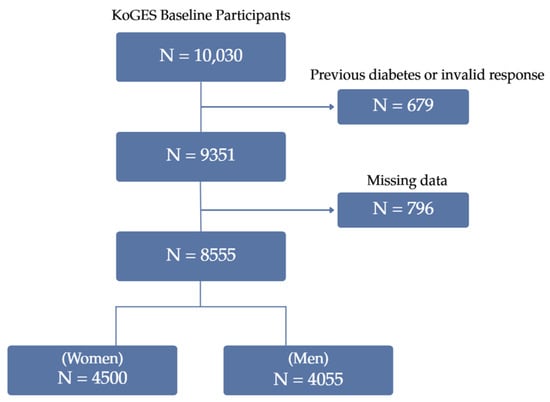
Of the 10,030 participants, 679 with a previous diagnosis of diabetes or an invalid response regarding diabetes history were excluded, followed by 80 participants with missing 120 min OGTT glucose values. Complete-case selection was then applied across all variables assessed during preprocessing, excluding 716 participants. Of these, 697 had missing values in one or more of the final model variables, and 19 had complete data for all final model variables but were missing light-intensity physical activity, a variable assessed during preprocessing and subsequently not retained. The complete-case criterion was applied once, before the final variable set was fixed, so that a single analytic sample was used throughout model development, evaluation, and interpretation; retaining these 19 participants would have increased the analytic sample by 0.2% (19 of 8574). The final analytic sample comprised 8555 participants (4055 men and 4500 women) (Figure 1). Variable-specific missingness is summarized in Table S3. Characteristics of included and excluded participants were compared using available observations and absolute standardized mean differences and are presented in Table S4. Data preprocessing, model development, performance evaluation, and model interpretation were conducted separately for men and women.

Figure 1. Flowchart of participant selection for the present study.

The outcome was defined by the plasma glucose concentration measured 120 min after the oral glucose load. Participants with a 120 min glucose concentration of ≥200 mg/dL were classified as the positive class, and those with a concentration of <200 mg/dL as the negative class. In the final sample, 253 of 4055 men (6.24%) and 225 of 4500 women (5.00%) were in the ≥200 mg/dL group.

This binary outcome was selected to identify participants whose 120 min glucose concentration fell within the diabetic diagnostic range. A positive model prediction therefore indicated classification into the ≥200 mg/dL group rather than a confirmed clinical diagnosis of diabetes. The <200 mg/dL comparison group included participants with both normal glucose tolerance and impaired glucose tolerance and should not be interpreted as a metabolically normal group. Participants were not excluded on the basis of fasting plasma glucose, because the objective was to identify individuals whose 120 min glucose concentration fell within the diabetic diagnostic range irrespective of fasting status. The ≥200 mg/dL group therefore included both individuals with isolated post-load hyperglycemia and individuals who would also meet fasting diagnostic criteria.

2.2. Variable Selection, Data Splitting, and Scaling

We selected 20 non-invasive predictors from the KoGES baseline dataset based on their clinical relevance and availability. They covered sociodemographic characteristics, lifestyle and physical activity, medical and family history, and anthropometric and body composition measurements.

The sociodemographic variables were age, marital status, occupation, educational level, and monthly household income. Age was recorded in completed years. Marital status was categorized as never married, married, widowed, separated, divorced, or other. Occupation was categorized as homemaker, office worker, agricultural worker, self-employed worker, sales worker, factory or production worker, professional worker, or other. Educational level was classified as elementary school or lower, middle school, high school, junior college, university, or graduate school or higher. Monthly household income was divided into eight categories: <0.5, 0.5–<1.0, 1.0–<1.5, 1.5–<2.0, 2.0–<3.0, 3.0–<4.0, 4.0–<6.0, and ≥6.0 million Korean won.

Alcohol consumption was recorded as never, former, or current drinking, and smoking status as never, former, occasional, or current regular smoking. Participants also reported the daily time spent lying down while awake, sitting, and engaging in moderate- and vigorous-intensity physical activity. Sitting included activities such as office work, driving, writing, and cooking. Moderate-intensity activities included brisk walking, mowing, swimming, and tennis. Vigorous-intensity activities included running, hiking, competitive sports, and physically demanding agricultural or forestry work. The same nine response categories were used for each activity measure: none, <30 min/day, 30–<60 min/day, 60–<90 min/day, 90 min–<2 h/day, 2–<3 h/day, 3–<4 h/day, 4–<5 h/day, and ≥5 h/day. These ordered categories were retained in the analysis.

Participants reported whether they had ever been diagnosed with hypertension or hyperlipidemia by a physician. Both variables were recorded as no or yes. For family history of diabetes, participants could report up to four affected relatives and their relationship to the participant. Family history was coded as present when at least one valid family-relationship response was recorded.

Waist and hip circumferences were based on the first recorded measurements and expressed in centimeters. Muscle mass and body fat mass were measured in kilograms using the InBody 3.0 body composition analyzer, and body mass index was calculated as weight in kilograms divided by height in meters squared. Seated systolic and diastolic blood pressure was measured in both arms, and mid-blood pressure was calculated by averaging the first systolic and diastolic measurements from the left and right arms. The same set of 20 variables was used for the male and female models.

Data were divided separately for men and women into training and test sets at an 80:20 ratio, with stratification by the binary outcome. The male training and test sets contained 3244 and 811 participants, including 202 and 51 participants with 2 h OGTT glucose levels ≥200 mg/dL, respectively. The corresponding female sets contained 3600 and 900 participants, of whom 180 and 45 had glucose levels ≥200 mg/dL.

The 20 predictor variables comprised continuous, ordinal, binary, and nominal categorical variables. Nominal categorical variables, including marital status, occupation, alcohol consumption, and smoking status, were represented using one-hot encoding. One category per nominal variable was used as the reference category. After one-hot encoding, the 20 original predictors corresponded to 33 columns in the model design matrix for each of the five algorithms in both the final male and female models. These comprised 17 indicator columns for the four nominal variables, seven standardized continuous variables, six standardized ordinal variables, and three binary variables. Variables with an inherent order, including education level, household income, and physical-activity duration categories, were retained as ordinal variables. Binary variables were coded as 0 or 1.

All preprocessing was fitted using the training data only. Continuous and ordinal variables were standardized using z-scores [12], whereas nominal categorical variables were one-hot encoded. The fitted preprocessing procedures were then applied to the test data. During cross-validation, preprocessing was refitted independently within each training fold to prevent information leakage.

2.3. Model Development and Optimization

Five classification algorithms with different modeling assumptions were used: logistic regression, Gaussian naive Bayes, random forest, XGBoost, and LightGBM. Logistic regression served as a conventional linear model and Gaussian naive Bayes as a probabilistic classifier. Random forest was included as a bagging-based ensemble, and XGBoost and LightGBM as gradient-boosting algorithms capable of modeling nonlinear relationships and interactions among variables [13,14,15]. All models were developed separately for men and women using the same set of variables.

In addition to the sex-specific models, pooled models were developed using the combined male and female development samples, with sex included as an additional predictor. A single selected threshold for each pooled model was subsequently applied to both male and female test participants.

Because the ≥200 mg/dL group constituted a small proportion of the study population, class weighting was applied to models supporting cost-sensitive learning [16]. Class weighting was chosen to address imbalance without generating synthetic training observations, consistent with the study’s focus on both prediction and interpretation of observed non-invasive profiles. SMOTE and SMOTE-Tomek were not used in the reported analyses. For logistic regression and random forest, class weights were set inversely proportional to class frequencies in the training data. For XGBoost and LightGBM, the ratio of negative to positive cases in the training data was used as the positive-class weight. Gaussian naive Bayes was trained without class weighting because its scikit-learn implementation does not provide a built-in class-weight option. Class weights were calculated from the training data only, and the test sets retained their original class distributions.

Hyperparameters were optimized for each algorithm in the sex-specific and pooled models using 100 Optuna trials [17], with mean F2 at a fixed threshold of 0.50 across five stratified validation folds as the objective. F2 emphasizes recall over precision, consistent with the aim of reducing false-negative predictions in the ≥200 mg/dL group. For the selected hyperparameters, out-of-fold probabilities were generated using the same fold assignments, and the threshold maximizing F2 was selected from 0.01 to 0.99 in increments of 0.01, with ties resolved in favor of the lowest threshold. These out-of-fold F2 values were treated as optimization statistics rather than independent performance estimates. Each model was then refitted on the full development sample, with its selected threshold fixed before test-set evaluation. Hyperparameter search spaces are presented in Table 1, and the selected hyperparameter settings for the final models are reported in Table S5.

Table 1. Hyperparameter search spaces used for model optimization.

Model	Hyperparameter	Search Space
Logistic regression	Regularization strength (C)	0.0001–10, log scale
	Solver	liblinear, lbfgs
	Penalty	L1 or L2 for liblinear; L2 for lbfgs
Gaussian naive Bayes	Variance smoothing	10−10–1, log scale
Random forest	Number of trees	100–500
	Maximum tree depth	3–10
	Minimum samples for node splitting	5–20
	Minimum samples per terminal node	2–10
XGBoost	Number of boosting iterations	100–500
	Maximum tree depth	2–6
	Learning rate	0.01–0.30
	Row subsampling ratio	0.60–1.00
	Feature subsampling ratio	0.60–1.00
	Minimum loss reduction (gamma)	0–5
LightGBM	Number of boosting iterations	100–500
	Maximum tree depth	2–7
	Number of leaves	8–32
	Learning rate	0.01–0.30
	Row subsampling ratio	0.60–1.00
	Feature subsampling ratio	0.60–1.00
	L1 regularization (reg_alpha)	0–5
	L2 regularization (reg_lambda)	0–5

2.4. Model Evaluation and Interpretation

Model performance was evaluated separately for men and women on the independent test sets. Discrimination was assessed using the area under the receiver operating characteristic curve (AUROC), and precision, recall, and F2 score were calculated at the model-specific thresholds selected from the out-of-fold training predictions. The F2 score was calculated as 5 × precision × recall/(4 × precision + recall). Given the low prevalence of the positive class, recall and F2 score were emphasized [18]. Additionally, for the sex-specific models, the area under the precision–recall curve (AUPRC) was calculated from predicted probabilities using trapezoidal integration, and specificity, negative predictive value (NPV), and confusion matrices were evaluated at the fixed development-selected thresholds.

For these measures, 95% confidence intervals were obtained from the 2.5th and 97.5th percentiles of 2000 nonparametric participant-level bootstrap samples, with the models and thresholds held fixed during resampling, so that the intervals quantify test-sample uncertainty conditional on the fitted models and selected thresholds. Sex-specific and pooled models were evaluated using the same held-out participants within each sex.

Robustness of the sex-specific models to data partitioning was assessed using five-fold stratified nested cross-validation repeated three times within the development sample. Within each outer training set, preprocessing, class-weight calculation where applicable, and the hyperparameter and threshold selection procedures described in Section 2.3 were repeated before model refitting. Outer validation observations were excluded from all fitting and selection steps, and the held-out test sets were not used in this analysis. Outer-fold mean performance and variation in repeat-specific means were summarized descriptively, without treating correlated fold estimates as independent observations.

To contextualize the screening implications of the reported performance, we considered a hypothetical strategy in which only participants with positive model predictions underwent OGTT. The proportion selected for OGTT was defined as (TP + FP)/N, the number of OGTTs per detected positive case as (TP + FP)/TP, and the proportion of positive cases missed as FN/(TP + FN). These quantities describe test allocation and case detection within the study sample, assuming that all selected participants complete OGTT. Testing all participants was used as a reference strategy rather than as a representation of routine clinical practice.

Model predictions were interpreted using SHAP [19]. Based on cooperative game theory, SHAP quantifies the contribution of each variable to an individual prediction relative to the model’s expected output. Positive SHAP values indicate contributions toward the ≥200 mg/dL group, negative values indicate contributions away from it, and the absolute magnitude reflects the strength of the contribution.

SHAP explainers were selected according to model structure: LinearExplainer for logistic regression, TreeExplainer for random forest, XGBoost, and LightGBM [20], and the model-agnostic KernelExplainer for Gaussian naive Bayes. A background sample of 150 participants was randomly selected without replacement from the development data and transformed using the fitted preprocessing pipeline. For Gaussian naive Bayes, KernelExplainer used 200 coalition samples per test observation. SHAP values were expressed on the log-odds scale for logistic regression, XGBoost, and LightGBM, and on the model-predicted probability scale for random forest and Gaussian naive Bayes.

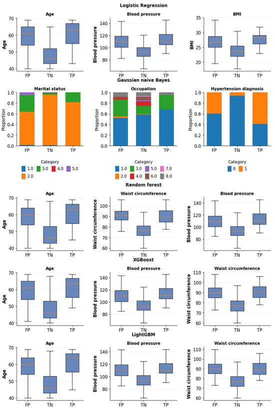
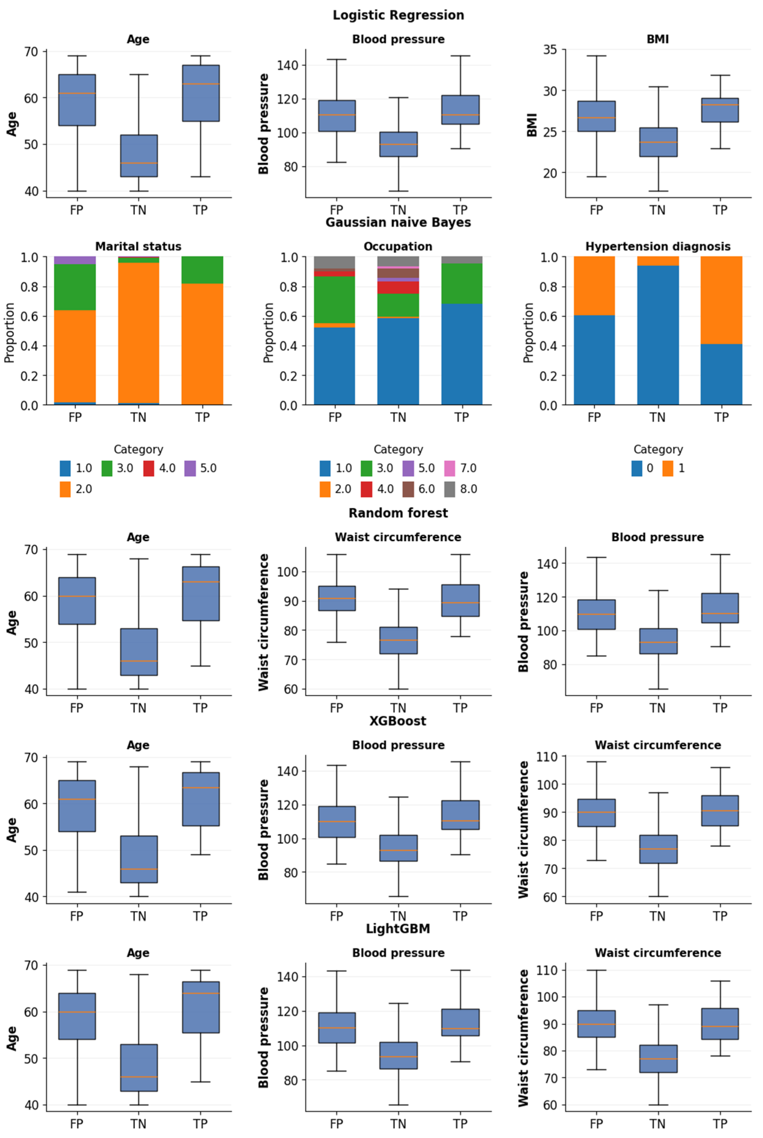
SHAP values were calculated for the independent test sets. Global variable importance was quantified as the mean absolute SHAP value, and the three highest-ranked variables were identified within each fitted model. Because the explained output scales differed across algorithms, absolute SHAP magnitudes were not compared quantitatively across models. SHAP dependence plots were used to examine the direction and pattern of their contributions separately for men and women. SHAP values were interpreted as explanations of model behavior rather than as evidence of causality. To descriptively characterize false-positive (FP) predictions, the distributions of the three highest-ranked variables were compared among FP, true-negative (TN), and true-positive (TP) participants in the test sets, as classified at the model-specific thresholds. These comparisons were presented graphically without inferential statistical testing.

The stability of SHAP-based predictor rankings was assessed using 1000 participant-level bootstrap resamples of each sex-specific held-out test set. For each resample, mean absolute SHAP values were recalculated from the saved participant-level SHAP values, and predictors were reranked within each model. Stability was summarized by the median and interquartile range of ranks and the proportion of resamples in which each originally top-three predictor remained among the top three. The fitted models and SHAP background samples were held fixed; this analysis therefore assessed ranking variability arising from the composition of the evaluation sample rather than from model refitting.

Among test participants with 120 min OGTT glucose concentrations <200 mg/dL, the proportions with concentrations of 140–199 mg/dL were compared between FP and TN groups. Between-group differences were expressed in percentage points, with 95% confidence intervals calculated using the Newcombe method based on Wilson score intervals. Analyses were performed using Python 3.13.16 (Python Software Foundation, Beaverton, OR, USA) with the following open-source packages: NumPy 2.1.3, pandas 2.2.3, SciPy 1.16.3, scikit-learn 1.6.1, Optuna 5.0.0, XGBoost 3.4.1, LightGBM 4.6.0, and SHAP 0.52.0.

A fixed random seed of 42 was used for the stratified train–test split, shuffled inner cross-validation folds, the Optuna tree-structured Parzen estimator sampler, and model random-state parameters where applicable. Bootstrap resampling and SHAP background sampling used NumPy random generators initialized with the same seed. The three repetitions of outer cross-validation used seeds of 1042, 1043, and 1044, respectively. For Kernel SHAP computations, NumPy seeds were set to 42 plus the zero-based starting observation index of each 50-observation processing chunk.

3. Results

3.1. Baseline Characteristics

The baseline characteristics of the 4055 men and 4500 women are compared in Table S1. Men and women differed in most sociodemographic, lifestyle, and anthropometric characteristics. Compared with men, women were slightly older and had higher mean body fat mass and body mass index, as well as higher prevalences of hypertension and a family history of diabetes. Men had greater mean waist circumference, muscle mass, and blood pressure and were more frequently current drinkers and current regular smokers. Hip circumference did not differ significantly between men and women (p = 0.208).

Baseline characteristics according to 120 min OGTT glucose status are presented separately for men and women in Table 2. In both sexes, participants with glucose levels of ≥200 mg/dL were older and had greater waist circumference, body fat mass, body mass index, and blood pressure and a higher prevalence of a family history of diabetes than those with glucose levels of <200 mg/dL. Among men, the distribution of recumbent time also differed between the glucose groups. Among women, differences were additionally observed in marital status, occupation, educational level, household income, alcohol consumption, moderate physical activity, hypertension, hyperlipidemia, and hip circumference. Muscle mass did not differ significantly according to OGTT glucose status in either men or women.

Table 2. Baseline characteristics according to 120 min OGTT glucose level, stratified by sex.

Characteristic	Men			Women
	<200 mg/dL (n = 3802)	≥200 mg/dL (n = 253)	p-Value	<200 mg/dL (n = 4275)	≥200 mg/dL (n = 225)	p-Value
Age, yr	51.1 (8.7)	52.8 (8.7)	0.004	52.0 (8.9)	57.5 (8.5)	<0.001
Marital status			0.734			<0.001
Living with spouse	3653 (96.1%)	242 (95.7%)		3644 (85.2%)	173 (76.9%)
Living alone	149 (3.9%)	11 (4.3%)		631 (14.8%)	52 (23.1%)
Occupation			0.212			0.028
Office worker	1464 (38.5%)	94 (37.2%)		524 (12.3%)	16 (7.1%)
Manual worker	1480 (38.9%)	90 (35.6%)		1099 (25.7%)	70 (31.1%)
Unemployed/Homemaker	858 (22.6%)	69 (27.3%)		2652 (62.0%)	139 (61.8%)
Educational level			0.835			<0.001
Middle school or lower	1590 (41.8%)	107 (42.3%)		2841 (66.5%)	176 (78.2%)
High school	1386 (36.5%)	95 (37.5%)		1152 (26.9%)	43 (19.1%)
College or higher	826 (21.7%)	51 (20.2%)		282 (6.6%)	6 (2.7%)
Household income (KRW million/month)			0.167			0.043
<2.0	2193 (57.7%)	140 (55.3%)		2930 (68.5%)	172 (76.4%)
2.0–<4.0	1251 (32.9%)	80 (31.6%)		1087 (25.4%)	42 (18.7%)
≥4.0	358 (9.4%)	33 (13.0%)		258 (6.0%)	11 (4.9%)
Alcohol consumption			0.064			0.022
Non-drinker	702 (18.5%)	32 (12.6%)		2991 (70.0%)	173 (76.9%)
Former drinker	372 (9.8%)	28 (11.1%)		122 (2.9%)	9 (4.0%)
Current drinker	2728 (71.8%)	193 (76.3%)		1162 (27.2%)	43 (19.1%)
Smoking status			0.319			0.408
Never smoker	734 (19.3%)	40 (15.8%)		4049 (94.7%)	217 (96.4%)
Former smoker	1190 (31.3%)	78 (30.8%)		58 (1.4%)	1 (0.4%)
Current smoker	1878 (49.4%)	135 (53.4%)		168 (3.9%)	7 (3.1%)
Recumbent time			0.006			0.235
None	1147 (30.2%)	56 (22.1%)		1376 (32.2%)	63 (28.0%)
<1 h/day	1223 (32.2%)	87 (34.4%)		1459 (34.1%)	75 (33.3%)
1–<2 h/day	759 (20.0%)	47 (18.6%)		753 (17.6%)	40 (17.8%)
≥2 h/day	673 (17.7%)	63 (24.9%)		687 (16.1%)	47 (20.9%)
Sitting time			0.100			0.079
None	224 (5.9%)	19 (7.5%)		217 (5.1%)	13 (5.8%)
<1 h/day	523 (13.8%)	29 (11.5%)		766 (17.9%)	49 (21.8%)
1–<2 h/day	613 (16.1%)	29 (11.5%)		938 (21.9%)	34 (15.1%)
≥2 h/day	2442 (64.2%)	176 (69.6%)		2354 (55.1%)	129 (57.3%)
Moderate physical activity			0.072			0.003
None	1826 (48.0%)	131 (51.8%)		2186 (51.1%)	126 (56.0%)
<1 h/day	940 (24.7%)	72 (28.5%)		1126 (26.3%)	68 (30.2%)
1–<2 h/day	507 (13.3%)	25 (9.9%)		538 (12.6%)	10 (4.4%)
≥2 h/day	529 (13.9%)	25 (9.9%)		425 (9.9%)	21 (9.3%)
Vigorous physical activity			0.239			0.501
None	2121 (55.8%)	156 (61.7%)		2710 (63.4%)	149 (66.2%)
<1 h/day	398 (10.5%)	26 (10.3%)		365 (8.5%)	14 (6.2%)
1–<2 h/day	224 (5.9%)	10 (4.0%)		183 (4.3%)	7 (3.1%)
≥2 h/day	1059 (27.9%)	61 (24.1%)		1017 (23.8%)	55 (24.4%)
Hypertension, n (%)	451 (11.9%)	40 (15.8%)	0.062	615 (14.4%)	77 (34.2%)	<0.001
Hyperlipidemia, n (%)	120 (3.2%)	9 (3.6%)	0.725	71 (1.7%)	9 (4.0%)	0.017
WC, cm	83.3 (7.6)	86.1 (8.1)	<0.001	81.0 (9.6)	86.1 (9.1)	<0.001
HC, cm	93.4 (5.7)	94.3 (6.9)	0.052	93.6 (6.1)	94.8 (6.4)	0.004
Muscle mass, kg	50.0 (6.1)	49.6 (6.7)	0.436	37.7 (4.3)	37.7 (4.7)	0.891
Body fat mass, kg	14.6 (4.9)	17.0 (5.7)	<0.001	18.7 (5.3)	21.3 (5.8)	<0.001
BMI, kg/m2	24.1 (2.9)	25.1 (3.5)	<0.001	24.8 (3.2)	26.3 (3.5)	<0.001
Blood pressure	101.5 (13.3)	106.2 (13.3)	<0.001	99.1 (14.9)	107.8 (14.7)	<0.001
Family history of diabetes, n (%)	353 (9.3%)	43 (17.0%)	<0.001	494 (11.6%)	38 (16.9%)	0.016

Values are presented as mean (SD) for continuous variables and n (%) for categorical variables. p-values were calculated using Welch’s t-test for continuous variables and the chi-square test for categorical variables, as appropriate. Percentages were calculated using non-missing observations within each sex. Selected categorical variables were regrouped solely for descriptive presentation in this table and were not used for model development. Model development used the original category coding described in Section 2.2. Abbreviations: BMI, body mass index; HC, hip circumference; WC, waist circumference.

3.2. Threshold Optimization

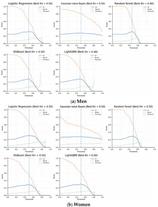
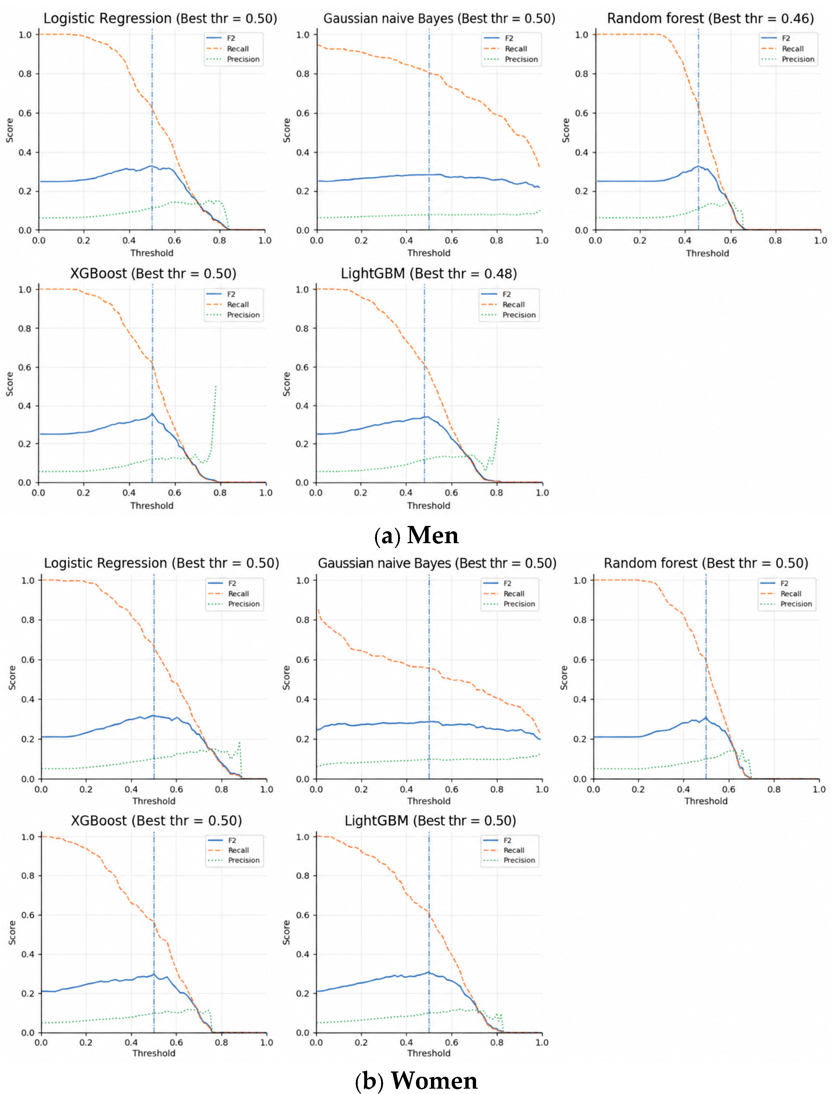
Model-specific probability thresholds were selected by maximizing the F2 score using out-of-fold predictions in the training data (Figure 2). In men, the selected thresholds were 0.50 for logistic regression, 0.50 for Gaussian naive Bayes, 0.46 for random forest, 0.50 for XGBoost, and 0.48 for LightGBM. In women, the selected threshold was 0.50 for all five models.

Figure 2. Out-of-fold threshold tuning curves for the five classification models in (a) men and (b) women. Vertical dash-dotted lines indicate the thresholds that maximized the F2 score in the training data.

3.3. Model Performance on the Held-Out Test Sets

The performance of the sex-specific models, with 95% confidence intervals, is presented in Table 3. In men, AUROC ranged from 0.579 to 0.665. Logistic regression had the highest observed AUROC (0.665; 95% CI, 0.599–0.730), precision (0.095), and F2 score (0.276; 95% CI, 0.193–0.353), whereas Gaussian naive Bayes had the highest recall (0.569). In women, AUROC ranged from 0.656 to 0.735. LightGBM had the highest observed AUROC (0.735; 95% CI, 0.658–0.806), random forest had the highest precision (0.098) and F2 score (0.300; 95% CI, 0.208–0.382), and logistic regression had the highest recall (0.644).

Table 3. Performance of the sex-specific models in the held-out test sets.

Sex	Model	AUROC	Precision	Recall	F2 Score
Men	Logistic Regression	0.665 (0.599–0.730)	0.095 (0.062–0.130)	0.529 (0.395–0.667)	0.276 (0.193–0.353)
Men	Gaussian naive Bayes	0.579 (0.496–0.659)	0.067 (0.045–0.091)	0.569 (0.429–0.704)	0.228 (0.160–0.292)
Men	Random forest	0.618 (0.544–0.686)	0.078 (0.048–0.108)	0.471 (0.339–0.610)	0.234 (0.158–0.308)
Men	XGBoost	0.634 (0.562–0.705)	0.091 (0.058–0.127)	0.471 (0.333–0.609)	0.257 (0.172–0.333)
Men	LightGBM	0.625 (0.556–0.694)	0.068 (0.040–0.099)	0.373 (0.250–0.510)	0.196 (0.123–0.271)
Women	Logistic Regression	0.725 (0.642–0.799)	0.091 (0.060–0.125)	0.644 (0.500–0.784)	0.292 (0.204–0.369)
Women	Gaussian naive Bayes	0.656 (0.577–0.729)	0.083 (0.051–0.117)	0.489 (0.333–0.640)	0.247 (0.160–0.326)
Women	Random forest	0.704 (0.623–0.778)	0.098 (0.062–0.134)	0.622 (0.469–0.762)	0.300 (0.208–0.382)
Women	XGBoost	0.720 (0.642–0.790)	0.092 (0.058–0.127)	0.578 (0.421–0.721)	0.281 (0.190–0.360)
Women	LightGBM	0.735 (0.658–0.806)	0.096 (0.062–0.133)	0.600 (0.443–0.743)	0.293 (0.203–0.375)

Values are point estimates with 95% percentile confidence intervals from 2000 participant-level bootstrap samples. Models and development-selected thresholds were held fixed during resampling.

In 5-fold stratified nested cross-validation repeated 3 times within the development sample, mean outer-fold AUROC ranged from 0.641 to 0.692 and mean F2 from 0.282 to 0.326 across the five male-specific models. The corresponding ranges for the five female-specific models were 0.688 to 0.726 and 0.277 to 0.301, respectively. The largest within-model range of repeat-specific mean AUROC was 0.024 in men and 0.025 in women; the corresponding values for F2 were 0.040 and 0.018, respectively.

The pooled models were evaluated separately in the same male and female held-out test sets (Table 4). In men, AUROC ranged from 0.507 to 0.629. Logistic regression had the highest observed AUROC (0.629; 95% CI, 0.560–0.699), precision (0.089), and F2 score (0.270; 95% CI, 0.192–0.343). In women, AUROC ranged from 0.664 to 0.727. Logistic regression had the highest observed AUROC (0.727; 95% CI, 0.646–0.801), precision (0.105), and F2 score (0.321; 95% CI, 0.230–0.401), whereas Gaussian naive Bayes had the highest recall (0.756).

Table 4. Performance of the pooled models evaluated separately in the male and female held-out test sets.

Sex	Model	AUROC	Precision	Recall	F2 Score
Men	Logistic Regression	0.629 (0.560–0.699)	0.089 (0.060–0.120)	0.549 (0.415–0.679)	0.270 (0.192–0.343)
Men	Gaussian naive Bayes	0.507 (0.428–0.581)	0.063 (0.041–0.085)	0.549 (0.411–0.681)	0.215 (0.149–0.277)
Men	Random forest	0.618 (0.547–0.690)	0.077 (0.046–0.111)	0.392 (0.259–0.528)	0.216 (0.137–0.293)
Men	XGBoost	0.598 (0.524–0.677)	0.077 (0.044–0.112)	0.353 (0.222–0.483)	0.206 (0.128–0.281)
Men	LightGBM	0.606 (0.532–0.682)	0.077 (0.048–0.109)	0.431 (0.300–0.566)	0.224 (0.149–0.301)
Women	Logistic Regression	0.727 (0.646–0.801)	0.105 (0.069–0.141)	0.667 (0.519–0.806)	0.321 (0.230–0.401)
Women	Gaussian naive Bayes	0.664 (0.592–0.730)	0.078 (0.053–0.105)	0.756 (0.621–0.878)	0.276 (0.201–0.347)
Women	Random forest	0.704 (0.630–0.771)	0.089 (0.057–0.122)	0.622 (0.471–0.760)	0.283 (0.196–0.362)
Women	XGBoost	0.716 (0.651–0.778)	0.091 (0.058–0.126)	0.578 (0.421–0.720)	0.280 (0.190–0.360)
Women	LightGBM	0.705 (0.635–0.771)	0.087 (0.056–0.121)	0.622 (0.469–0.762)	0.280 (0.195–0.358)

Values are point estimates with 95% percentile confidence intervals calculated as described for Table 3. Pooled models were evaluated in the same test participants, with a single development-selected threshold per model applied to both sex subgroups.

Compared with the corresponding pooled models, the sex-specific models had numerically higher AUROC values for logistic regression, Gaussian naive Bayes, XGBoost, and LightGBM in men. In women, AUROC was numerically higher for the sex-specific XGBoost and LightGBM models and for the pooled logistic regression and Gaussian naive Bayes models. Random forest AUROC values were identical at the reported three-decimal precision in both sexes.

3.4. Additional Performance Measures and Classification Errors

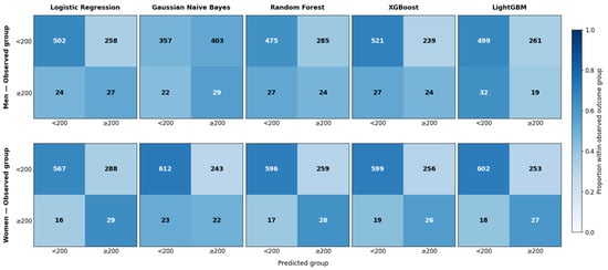
Additional performance measures for the sex-specific models are presented in Table 5, and their confusion matrices are shown in Figure 3. In men, AUPRC ranged from 0.089 to 0.132, specificity from 0.470 to 0.686, and NPV from 0.940 to 0.954. Logistic regression had the highest observed AUPRC (0.132; 95% CI, 0.072–0.214). At the development-selected thresholds, the models classified 22–32 of the 51 positive participants as negative and 239–403 of the 760 negative participants as positive.

Table 5. Additional performance measures of the sex-specific models in the held-out test sets.

Sex	Model	AUPRC	Specificity	NPV
Men	Logistic Regression	0.132 (0.072–0.214)	0.661 (0.626–0.694)	0.954 (0.936–0.971)
Men	Gaussian naive Bayes	0.089 (0.056–0.141)	0.470 (0.433–0.506)	0.942 (0.917–0.963)
Men	Random forest	0.126 (0.067–0.224)	0.625 (0.590–0.659)	0.946 (0.926–0.964)
Men	XGBoost	0.117 (0.068–0.193)	0.686 (0.652–0.718)	0.951 (0.933–0.967)
Men	LightGBM	0.120 (0.069–0.220)	0.657 (0.621–0.688)	0.940 (0.919–0.959)
Women	Logistic Regression	0.129 (0.075–0.232)	0.663 (0.631–0.694)	0.973 (0.958–0.985)
Women	Gaussian naive Bayes	0.078 (0.050–0.139)	0.716 (0.685–0.746)	0.964 (0.948–0.978)
Women	Random forest	0.106 (0.063–0.165)	0.697 (0.665–0.728)	0.972 (0.959–0.984)
Women	XGBoost	0.133 (0.070–0.214)	0.701 (0.669–0.731)	0.969 (0.955–0.982)
Women	LightGBM	0.162 (0.086–0.262)	0.704 (0.671–0.734)	0.971 (0.957–0.984)

Values are point estimates with 95% percentile confidence intervals calculated as described for Table 3. AUPRC, area under the precision–recall curve; NPV, negative predictive value.

Figure 3. Confusion matrices of the sex-specific models in the held-out test sets.

In women, AUPRC ranged from 0.078 to 0.162, specificity from 0.663 to 0.716, and NPV from 0.964 to 0.973. LightGBM had the highest observed AUPRC (0.162; 95% CI, 0.086–0.262). At the development-selected thresholds, the models classified 16–23 of the 45 positive participants as negative and 243–288 of the 855 negative participants as positive.

3.5. SHAP-Based Variable Importance

For each model, the three highest-ranked variables based on mean absolute SHAP values were examined to identify variables consistently emphasized across models within each sex.

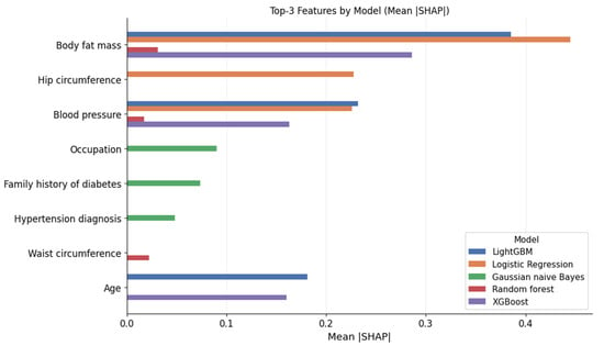
In men, body fat mass ranked among the top three variables in four models and ranked first in logistic regression, random forest, XGBoost, and LightGBM. Blood pressure ranked among the top three in four models, and age in two models. Waist circumference appeared only in random forest, and hip circumference appeared only in logistic regression. Occupation, family history of diabetes, and hypertension history appeared only in Gaussian naive Bayes (Figure 4).

Figure 4. Top three features identified by mean absolute SHAP values for each model in men.

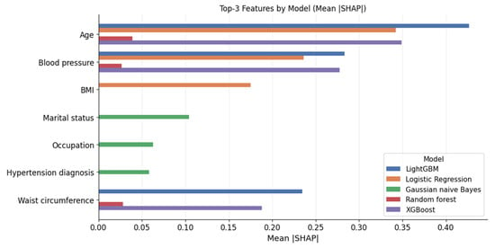
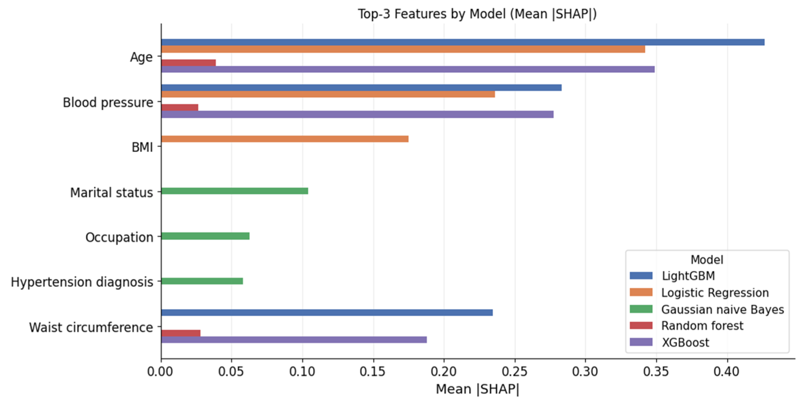
In women, age and blood pressure ranked among the top three variables in four models. Waist circumference appeared in three models, and body mass index appeared only in logistic regression. Marital status, occupation, and hypertension history appeared only in Gaussian naive Bayes (Figure 5).

Figure 5. Top three features identified by mean absolute SHAP values for each model in women.

Across 1000 bootstrap resamples of the held-out test participants, 27 of the 30 originally top three model–predictor combinations remained among the top three in every resample. The exceptions were hypertension history in the male Gaussian naive Bayes model (77.1%), blood pressure in the male random forest model (86.7%), and waist circumference in the female LightGBM model (96.9%). Body fat mass in men and age in women each had a median rank of 1 (IQR, 1–1) in logistic regression, random forest, XGBoost, and LightGBM. These results support the persistence of the main predictor patterns under resampling of the evaluation participants, conditional on the fitted models, and do not address variability that would arise from independently retrained models.

3.6. Directional Patterns of SHAP Contributions

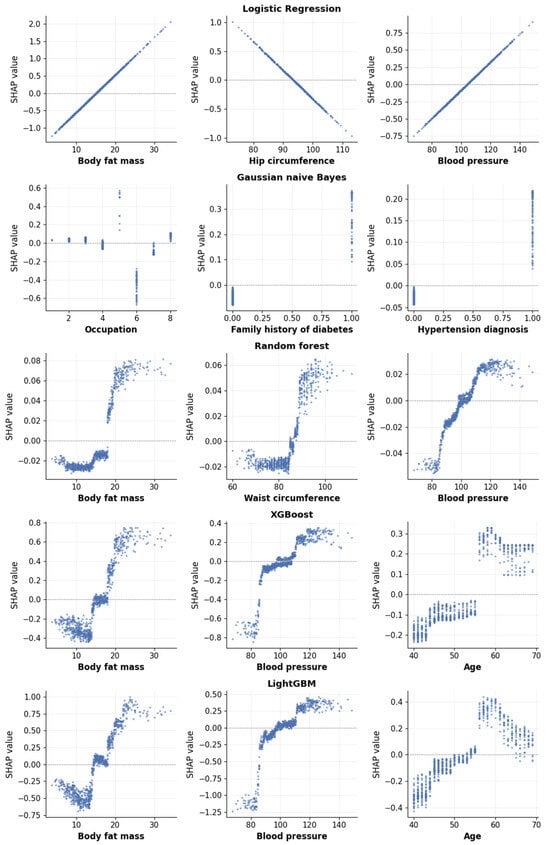
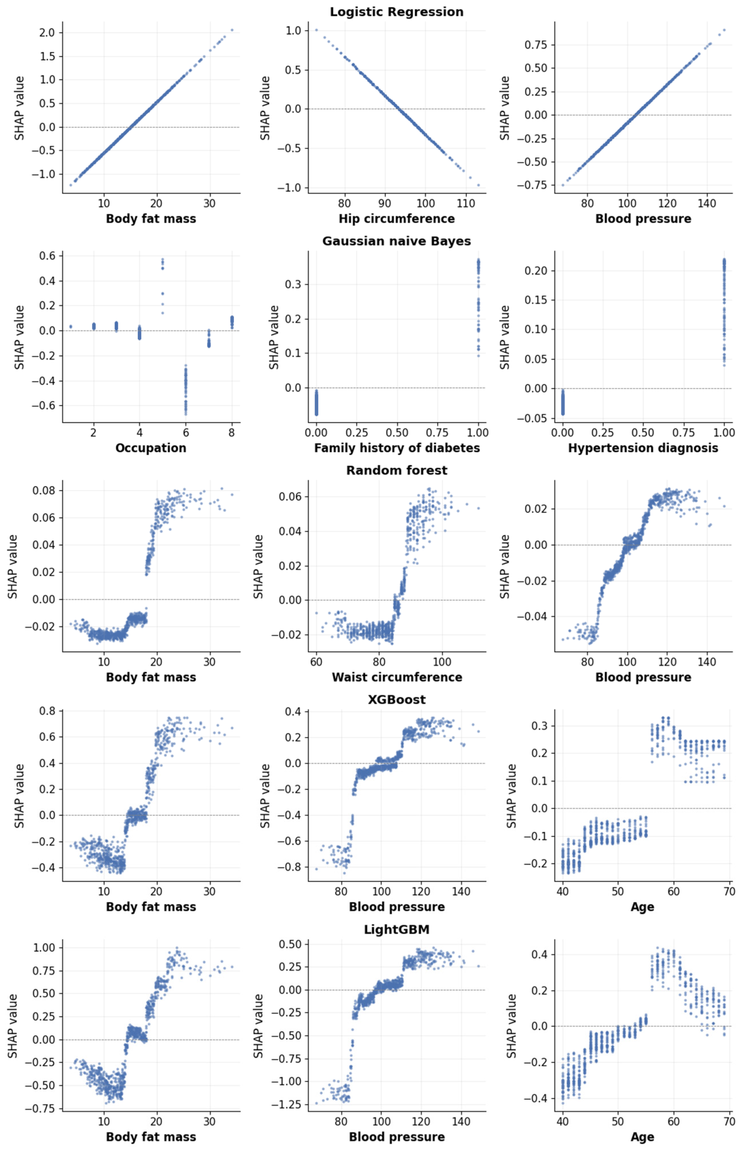
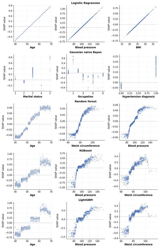
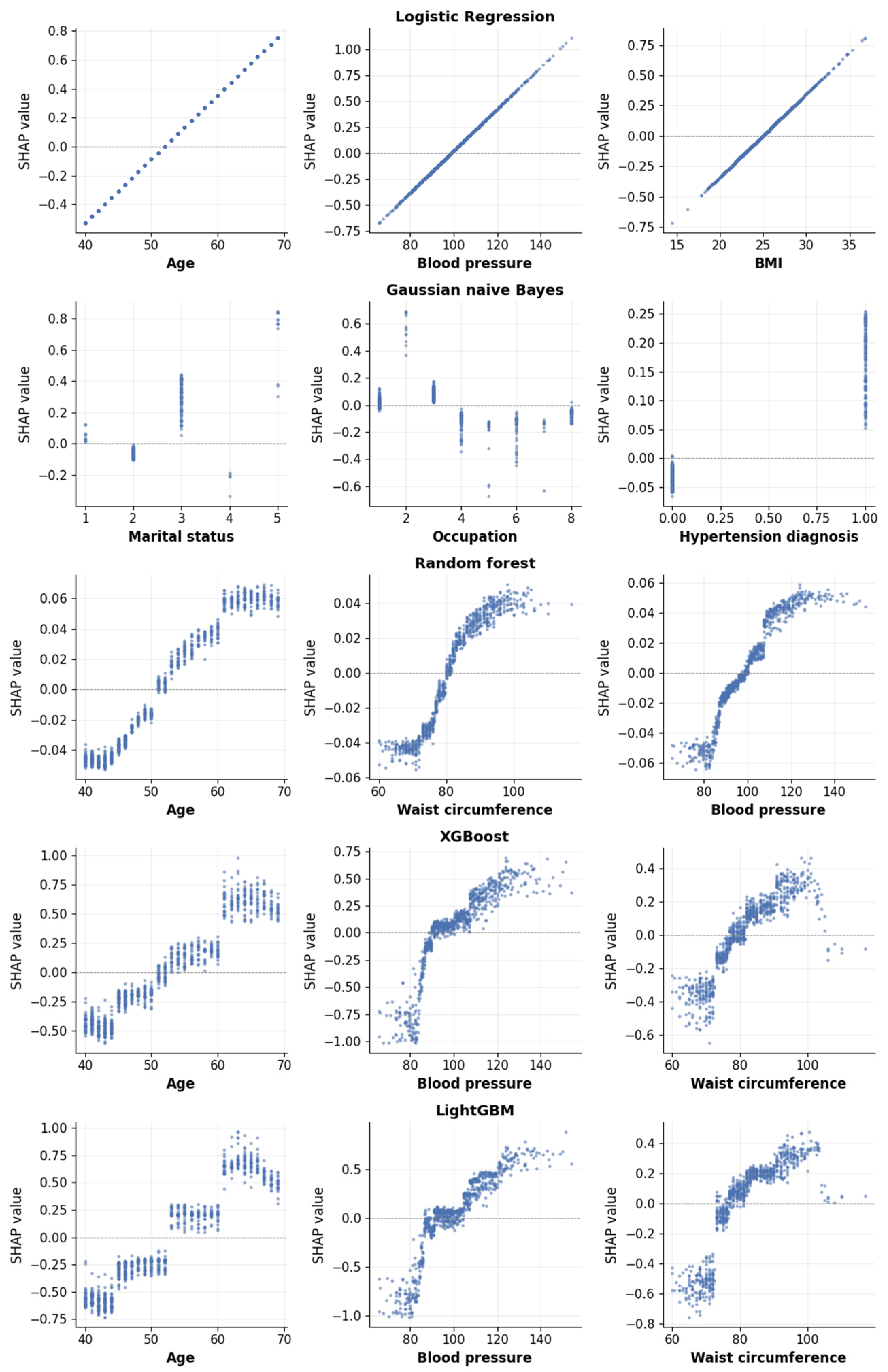
SHAP dependence plots for the three highest-ranked variables of each model are presented in Figure 6 (men) and Figure 7 (women).

Figure 6. SHAP dependence plots for the three highest-ranked variables in each model among men.

Figure 7. SHAP dependence plots for the three highest-ranked variables in each model among women.

In men, higher body fat mass and blood pressure generally corresponded to more positive SHAP values across the models in which these variables ranked highly (Figure 6). Logistic regression showed approximately linear positive relationships for body fat mass and blood pressure and a negative relationship for hip circumference. In random forest, XGBoost, and LightGBM, body fat mass and blood pressure exhibited nonlinear patterns, shifting from predominantly negative to positive contributions as their values increased. Higher waist circumference also corresponded to more positive SHAP values in random forest. In XGBoost and LightGBM, age showed nonlinear patterns, with contributions shifting from negative to positive around the mid-50s and declining at higher ages. In Gaussian naive Bayes, occupation, family history of diabetes, and hypertension history showed distinct contributions across categories, with the presence of a family history of diabetes or hypertension generally contributing positively.

In women, higher age and blood pressure generally corresponded to more positive SHAP values across the four models in which these variables ranked highly (Figure 7). Logistic regression showed approximately linear positive relationships for age, blood pressure, and body mass index, whereas random forest, XGBoost, and LightGBM showed nonlinear patterns in the contributions of age and blood pressure, with shapes varying across models. In random forest, XGBoost, and LightGBM, waist circumference generally shifted from predominantly negative to positive contributions as its value increased. However, contributions declined at the upper ends of the age and waist circumference ranges in XGBoost and LightGBM. Marital status, occupation, and hypertension history in Gaussian naive Bayes showed distinct contributions across categories, with the presence of hypertension generally contributing positively.

3.7. Characteristics of False-Positive Predictions

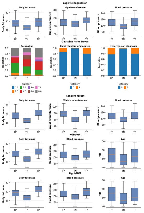
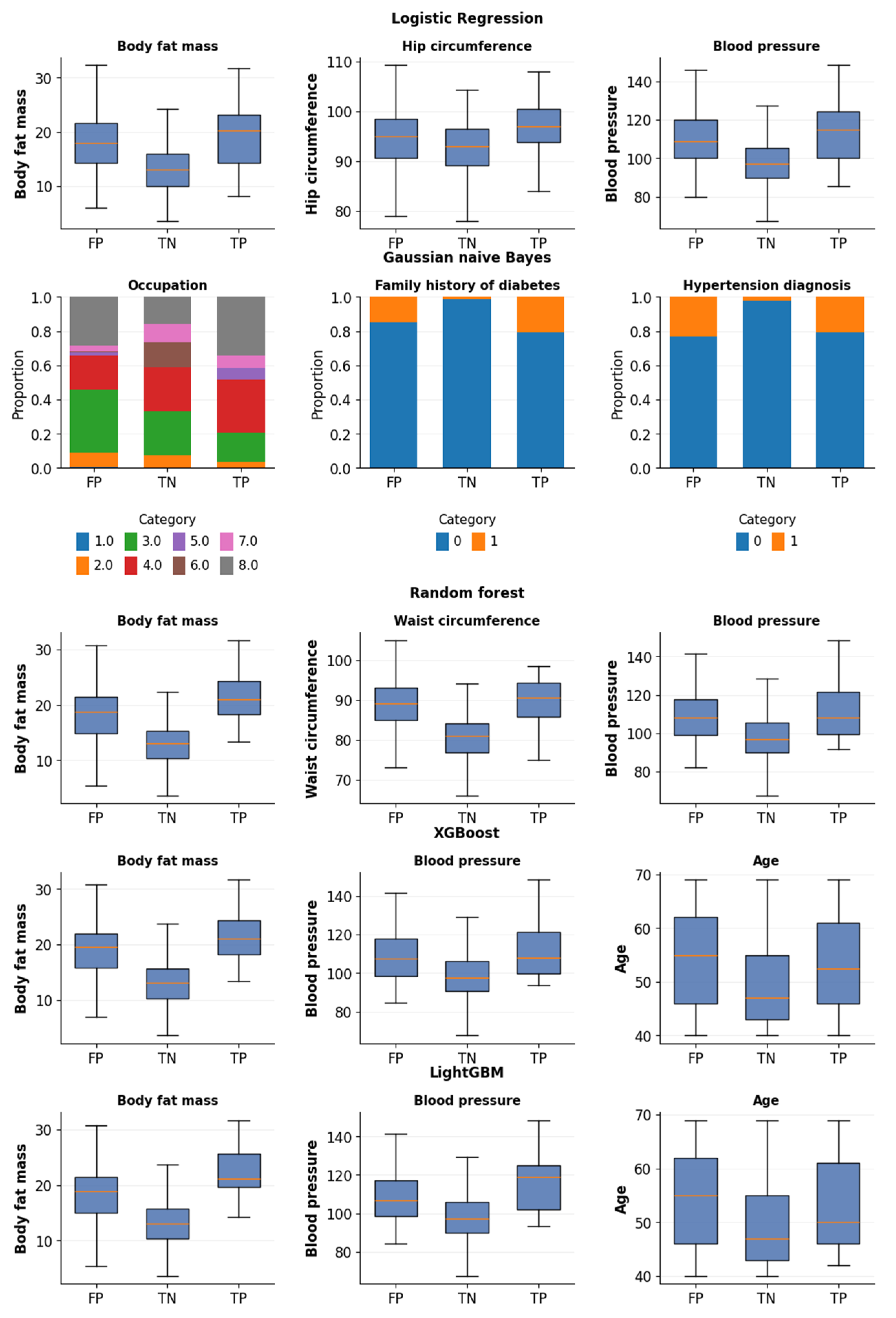
The distributions of the three highest-ranked variables for each model were compared among FP, TN, and TP participants (Figure 8 and Figure 9). In both sexes, FP participants generally showed variable distributions that differed from those of TN participants and overlapped with or were intermediate to those of TP participants. Similar patterns were observed for continuous and categorical variables, although their magnitude and consistency varied across models.

Figure 8. Distribution of the top three variables by prediction group in men. The yellow line in each box is the median. Occupation codes: 1 = homemaker, 2 = office, 3 = agricultural, 4 = self-employed, 5 = sales, 6 = production, 7 = professional, 8 = other. Family history of diabetes and hypertension history: 0 = no, 1 = yes. FP, false positive; TN, true negative; TP, true positive.

Figure 9. Distribution of the top three variables by prediction group in women. The yellow line in each box is the median. Marital status codes: 1 = never married, 2 = married, 3 = widowed, 4 = separated, 5 = divorced (“other” absent in this sample). Occupation codes: 1 = homemaker, 2 = office, 3 = agricultural, 4 = self-employed, 5 = sales, 6 = production, 7 = professional, 8 = other. Hypertension history: 0 = no, 1 = yes. FP, false positive; TN, true negative; TP, true positive.

Among participants with 120min OGTT glucose concentrations <200 mg/dL, the proportion with concentrations of 140–199 mg/dL, corresponding to the impaired glucose tolerance range, was higher in the FP group than in the TN group across all five models in both sexes. These proportions ranged from 25.8% to 33.3% versus 16.2% to 17.9% in men and from 30.1% to 31.6% versus 20.1% to 20.8% in women. Model-specific proportions and between-group differences are presented in Table S2.

4. Discussion

This study evaluated whether sex-specific models based on non-invasive variables could identify individuals with 120 min OGTT glucose concentrations of ≥200 mg/dL. Overall performance was modest, and no model consistently outperformed the others across sexes and evaluation metrics. Logistic regression achieved the highest AUROC and F2 score in men, whereas Gaussian naive Bayes showed the highest recall. In women, LightGBM achieved the highest AUROC, random forest achieved the highest F2 score, and logistic regression showed the highest recall. Thus, the more complex machine learning models did not show a consistent advantage over the conventional statistical model. Discrimination was generally higher in the female models (AUROC, 0.656–0.735) than in the male models (0.579–0.665).

The pooled models were trained on 6844 participants, compared with 3244 and 3600 participants for the male- and female-specific models, respectively. Despite this difference in development sample size, neither modeling approach consistently yielded higher point estimates across algorithms and performance metrics. These findings do not establish statistical equivalence or isolate the effect of training sample size, because sample size and population composition differed together. Consistent with the study’s focus on sex-related predictive patterns, subsequent interpretation centered on the sex-specific models. This approach allowed predictor contributions to be examined within each sex without imposing a single shared fitted relationship across men and women. The emphasis on sex-specific models therefore reflects the interpretive aim of the study rather than demonstrated predictive superiority over pooled models.

The observed results did not show a consistent performance advantage of the more complex algorithms over logistic regression with the available predictors. A systematic review comparing logistic regression and machine learning approaches similarly found no consistent performance advantage of machine learning in clinical prediction studies [21]. Previous studies predicting OGTT-defined glucose abnormalities used fasting glucose, lipid profiles, and other laboratory measurements that provide more direct information on glucose metabolism [6,7]. In contrast, the present study deliberately used variables obtainable without blood testing. This design reduced reliance on laboratory measurements but did not establish that the resulting models were sufficiently accurate for clinical screening. Although the low prevalence of the positive class contributes to low precision, it does not remove the practical burden of false-positive predictions. Likewise, optimizing F2 places greater emphasis on recall but does not ensure a clinically acceptable proportion of missed cases. Probability calibration was not assessed; therefore, the numerical thresholds should not be interpreted as absolute clinical risk thresholds. The SHAP analyses describe contributions to the fitted models’ predictions rather than changes in an individual’s absolute clinical risk.

The practical implications can be illustrated by comparing model-based selection with a hypothetical strategy of performing OGTT in all test participants. For the male-specific logistic regression model, approximately 35% of participants would be selected for OGTT, requiring approximately 11 OGTTs per detected positive case, compared with approximately 16 when testing all male participants. However, model-based selection would miss approximately 47% of positive cases. For the female-specific random forest model, approximately 32% would be selected, requiring approximately 10 OGTTs per detected positive case rather than 20 when testing all female participants, while missing approximately 38% of positive cases. These examples illustrate a trade-off between fewer OGTTs and incomplete case detection, rather than established clinical benefit. The findings therefore do not support using a negative model prediction alone to exclude further glucose assessment.

The SHAP analyses revealed differences in the relative prominence of variables between women and men. In women, age ranked among the top three variables in four models, with increasing age generally contributing toward prediction of the ≥200 mg/dL group. The prominence of age in the female models is consistent with previous literature on aging and glucose metabolism [8,9]. However, the present analysis does not establish why age ranked more prominently in the female models or whether this difference reflects sex-specific physiology. In contrast, the male models consistently emphasized adiposity-related information: body fat mass ranked among the top three variables in four models and ranked first in four, and waist circumference was prominent in random forest. Higher values of these measures generally contributed toward positive predictions, potentially reflecting the metabolic burden of excess adiposity [8,9]. This interpretation is supported by a prospective study reporting that predicted fat mass and waist circumference were more strongly associated with incident type 2 diabetes than BMI in men [22].

Blood pressure was a shared variable, ranking among the top three in four male models and four female models, with higher values generally contributing toward positive predictions. Its repeated importance may reflect overlapping cardiometabolic abnormalities, consistent with prospective evidence linking elevated blood pressure to subsequent diabetes development [23]. Other variables showed more model-specific patterns; for example, occupation, family history of diabetes, and hypertension history in men and marital status, occupation, and hypertension history in women ranked highly only in Gaussian naive Bayes. Overall, the SHAP findings suggest that the fitted male and female models placed different relative emphasis on age and adiposity-related information, while blood pressure contributed to predictions in both sexes. These patterns offer an exploratory view of how non-invasive characteristics contribute to predictions within each sex, without establishing the physiological mechanisms underlying the observed differences. Correlations among body fat mass, body mass index, and waist circumference may also influence their relative SHAP rankings, so these rankings should be interpreted in the context of related adiposity measures rather than as isolated contributions. The bootstrap analysis described in Section 3.5 indicates that these rankings were stable to resampling of the evaluation participants, but it does not assess how they would vary across independently trained models. The sex-specific patterns reported here should therefore be understood as properties of the fitted models rather than as established differences in predictor importance between men and women.

Beyond predicting whether 120 min glucose concentrations exceeded the study threshold, this study examined the non-invasive characteristics underlying those predictions. The OGTT measures the glycemic response to a glucose load, but its result alone does not explain how an individual’s anthropometric, demographic, and lifestyle characteristics relate to that response. By integrating these characteristics and examining their contributions using SHAP, the present analysis provided a complementary view of the profiles associated with model-predicted post-load hyperglycemia. The recurring prominence of adiposity-related measures in men, age in women, and blood pressure in both sexes highlighted patterns that could be considered alongside the OGTT result.

The FP analysis further showed that participants below the glucose threshold could share non-invasive characteristics with participants in the ≥200 mg/dL group. This overlap helps explain why the models produced positive predictions despite glucose concentrations below the threshold and illustrates the incomplete correspondence between non-invasive risk profiles and measured glucose status. Clinically, such profiles may provide a starting point for reviewing measured risk factors and discussing appropriate lifestyle measures, with advice guided by clinical assessment rather than the model classification alone. These findings concern predictive associations and model behavior; they do not establish the causes of elevated glucose or the effectiveness of model-guided counseling.

Hyperglycemia has been associated with adverse outcomes in other clinical contexts, including progression to frailty in hypertensive older adults with glucose concentrations below the diagnostic threshold for diabetes [24], and cognitive impairment and reduced gait speed in heart failure with preserved ejection fraction [25,26]. These populations differ from the present community-based cohort, and this study did not assess clinical outcomes. They nonetheless support the value of identifying individuals whose glucose falls within the diabetic range, including those detectable only after a glucose load.

Several limitations should be considered. First, this study used baseline data collected in 2001–2002 from adults aged 40–69 years in two Korean communities; therefore, the findings reflect a specific temporal, geographic, and age context and may not be generalizable to more contemporary or diverse populations. Second, the outcome was defined as a binary classification of 120 min OGTT glucose concentrations (<200 vs. ≥200 mg/dL) because the primary objective was to identify individuals whose glucose concentration was within the diabetic diagnostic range. Consequently, the <200 mg/dL group included participants with both normal glucose tolerance and impaired glucose tolerance and should not be interpreted as a metabolically normal group. The present models therefore cannot distinguish individuals with impaired glucose tolerance from those with normal glucose tolerance, despite the different clinical implications of these conditions. In addition, participants were not selected on the basis of fasting glucose, and the models should therefore not be interpreted as identifying isolated post-load hyperglycemia specifically. A three-category analysis would represent a distinct multiclass prediction problem and would require separate model development and validation. Future studies with larger numbers of outcome events should distinguish normal glucose tolerance (<140 mg/dL), impaired glucose tolerance (140–199 mg/dL), and diabetic range glucose concentrations (≥200 mg/dL).

Third, the held-out test sets contained only 51 male and 45 female positive cases, limiting the precision of performance estimates. Bootstrap confidence intervals and repeated nested cross-validation were used to characterize test-sample uncertainty and sensitivity to data partitioning, respectively. Nevertheless, these internal analyses do not replace external validation.

Finally, body composition measurements required an InBody analyzer, which may limit implementation in settings without access to this equipment. These variables were included to examine the predictive and interpretive information available from non-invasive characteristics, rather than to develop a minimal-input tool requiring no specialized equipment. Performance without body composition measurements was not evaluated, and applicability in settings where these measurements are unavailable remains to be established.

Despite these limitations, this study has several strengths. First, the models integrated non-invasive characteristics obtainable without blood testing, allowing us to evaluate the predictive information available from demographic, anthropometric, and lifestyle measures. Second, sex-specific analyses using the same predictor set enabled the examination of similarities and differences in predictive patterns between men and women. Third, the comparison of multiple algorithms allowed us to identify characteristics repeatedly emphasized across models rather than relying on the interpretation of a single algorithm. Finally, the combined SHAP and FP analyses provided insight into both the characteristics underlying positive predictions and their overlap between participants above and below the glucose threshold. These analyses extended the study beyond classification performance by examining how non-invasive profiles relate to model-predicted glucose status, providing complementary context for considering OGTT results alongside an individual’s measured risk factors.

In conclusion, sex-specific models using non-invasive variables showed modest ability to predict 120 min OGTT glucose concentrations of ≥200 mg/dL, and complex machine learning algorithms did not consistently outperform logistic regression. Beyond predictive performance, the SHAP analyses identified recurring sex-specific patterns in the characteristics contributing to model predictions, while the FP analyses showed that participants below the glucose threshold could share non-invasive profiles with those in the diabetic-range group. These findings suggest a potential role for explainable models in contextualizing OGTT results and supporting the review of clinically relevant risk factors, rather than determining the need for OGTT on their own. Such interpretation concerns predictive associations rather than the causes of elevated glucose. Further validation should assess the reproducibility of these patterns and whether presenting model explanations adds value to clinical risk-factor assessment and patient counseling.

References

- GBD 2021 Diabetes Collaborators. Global, regional, and national burden of diabetes from 1990 to 2021, with projections of prevalence to 2050: A systematic analysis for the Global Burden of Disease Study 2021. Lancet 2023, 402, 203–234. [Google Scholar] [CrossRef] [Scilit] [PubMed]
- American Diabetes Association Professional Practice Committee for Diabetes. Diagnosis and Classification of Diabetes: Standards of Care in Diabetes—2026. Diabetes Care 2026, 49, S27–S49. [Google Scholar] [CrossRef] [Scilit] [PubMed]
- Awad, K.; Kakkola, L.; Julkunen, I. High Glucose Increases Lactate and Induces the Transforming Growth Factor Beta-Smad 1/5 Atherogenic Pathway in Primary Human Macrophages. Biomedicines 2024, 12, 1575. [Google Scholar] [CrossRef] [Scilit] [PubMed]
- DECODE Study Group. Glucose tolerance and mortality: Comparison of WHO and American Diabetes Association diagnostic criteria. Lancet 1999, 354, 617–621. [Google Scholar] [CrossRef] [Scilit]
- Sacks, D.B. A1C versus glucose testing: A comparison. Diabetes Care 2011, 34, 518–523. [Google Scholar] [CrossRef] [Scilit] [PubMed]
- Babbar, R.; Heni, M.; Peter, A.; Hrabě de Angelis, M.; Häring, H.-U.; Fritsche, A.; Preissl, H.; Schölkopf, B.; Wagner, R. Prediction of glucose tolerance without an oral glucose tolerance test. Front. Endocrinol. 2018, 9, 82. [Google Scholar] [CrossRef] [Scilit] [PubMed]
- Wang, L.; Xie, J.; Gu, Z.; Miao, X.; Ma, L.; Yan, S.; Gong, Y.; Li, C.; Sun, B.; Ruan, Y. Predicting isolated impaired glucose tolerance without oral glucose tolerance test using machine learning in Chinese Han men. Front. Endocrinol. 2025, 16, 1514397. [Google Scholar] [CrossRef] [Scilit] [PubMed]
- Tramunt, B.; Smati, S.; Grandgeorge, N.; Lenfant, F.; Arnal, J.-F.; Montagner, A.; Gourdy, P. Sex differences in metabolic regulation and diabetes susceptibility. Diabetologia 2020, 63, 453–461. [Google Scholar] [CrossRef] [Scilit] [PubMed]
- Kautzky-Willer, A.; Harreiter, J.; Pacini, G. Sex and gender differences in risk, pathophysiology and complications of type 2 diabetes mellitus. Endocr. Rev. 2016, 37, 278–316. [Google Scholar] [CrossRef] [Scilit] [PubMed]
- de Hond, A.A.H.; Leeuwenberg, A.M.; Hooft, L.; Kant, I.M.J.; Nijman, S.W.J.; van Os, H.J.A.; Aardoom, J.J.; Debray, T.P.A.; Schuit, E.; van Smeden, M.; et al. Guidelines and quality criteria for artificial intelligence-based prediction models in healthcare: A scoping review. npj Digit. Med. 2022, 5, 2. [Google Scholar] [CrossRef] [Scilit] [PubMed]
- Kim, Y.; Han, B.G.; KoGES Group. Cohort Profile: The Korean Genome and Epidemiology Study (KoGES) Consortium. Int. J. Epidemiol. 2017, 46, e20. [Google Scholar] [CrossRef] [Scilit] [PubMed]
- StandardScaler—Scikit-learn Documentation. Available online: https://scikit-learn.org/stable/modules/generated/sklearn.preprocessing.StandardScaler.html (accessed on 8 September 2026).
- Breiman, L. Random Forests. Mach. Learn. 2001, 45, 5–32. [Google Scholar] [CrossRef] [Scilit]
- Chen, T.; Guestrin, C. XGBoost: A Scalable Tree Boosting System. In Proceedings of the 22nd ACM SIGKDD International Conference on Knowledge Discovery and Data Mining, San Francisco, CA, USA, 13–17 August 2016; pp. 785–794. [Google Scholar]
- Ke, G.; Meng, Q.; Finley, T.; Wang, T.; Chen, W.; Ma, W.; Ye, Q.; Liu, T.Y. LightGBM: A Highly Efficient Gradient Boosting Decision Tree. Adv. Neural Inf. Process. Syst. 2017, 30, 3146–3154. [Google Scholar]
- He, H.; Garcia, E.A. Learning from Imbalanced Data. IEEE Trans. Knowl. Data Eng. 2009, 21, 1263–1284. [Google Scholar] [CrossRef] [Scilit]
- Akiba, T.; Sano, S.; Yanase, T.; Ohta, T.; Koyama, M. Optuna: A Next-Generation Hyperparameter Optimization Framework. In Proceedings of the 25th ACM SIGKDD International Conference on Knowledge Discovery and Data Mining, Anchorage, AK, USA, 4–8 August 2019; pp. 2623–2631. [Google Scholar]
- Saito, T.; Rehmsmeier, M. The Precision–Recall Plot is More Informative than the ROC Plot When Evaluating Binary Classifiers on Imbalanced Datasets. PLoS ONE 2015, 10, e0118432. [Google Scholar] [CrossRef] [Scilit] [PubMed]
- Lundberg, S.M.; Lee, S.I. A Unified Approach to Interpreting Model Predictions. Adv. Neural Inf. Process. Syst. 2017, 30, 4765–4774. [Google Scholar]
- Lundberg, S.M.; Erion, G.; Chen, H.; DeGrave, A.; Prutkin, J.M.; Nair, B.; Katz, R.; Himmelfarb, J.; Bansal, N.; Lee, S.-I. From Local Explanations to Global Understanding with Explainable AI for Trees. Nat. Mach. Intell. 2020, 2, 56–67. [Google Scholar] [CrossRef] [Scilit] [PubMed]
- Christodoulou, E.; Ma, J.; Collins, G.S.; Steyerberg, E.W.; Verbakel, J.Y.; Van Calster, B. A systematic review shows no performance benefit of machine learning over logistic regression for clinical prediction models. J. Clin. Epidemiol. 2019, 110, 12–22. [Google Scholar] [CrossRef] [Scilit] [PubMed]
- Lee, D.H.; Keum, N.; Hu, F.B.; Orav, E.J.; Rimm, E.B.; Willett, W.C.; Giovannucci, E.L. Comparison of the association of predicted fat mass, body mass index, and other obesity indicators with type 2 diabetes risk: Two large prospective studies in US men and women. Eur. J. Epidemiol. 2018, 33, 1113–1123. [Google Scholar] [CrossRef] [Scilit] [PubMed]
- Emdin, C.A.; Anderson, S.G.; Woodward, M.; Rahimi, K. Usual blood pressure and risk of new-onset diabetes: Evidence from 4.1 million adults and a meta-analysis of prospective studies. J. Am. Coll. Cardiol. 2015, 66, 1552–1562. [Google Scholar] [PubMed]
- Mone, P.; De Gennaro, S.; Frullone, S.; Marro, A.; Santulli, G. Hyperglycemia drives the transition from pre-frailty to frailty: The Monteforte study. Eur. J. Intern. Med. 2023, 111, 135–137. [Google Scholar] [CrossRef] [Scilit] [PubMed]
- Mone, P.; Ciccarelli, M.; Jankauskas, S.S.; Picone, F.; Guerra, G.; Testa, G.; Moccia, F.; Magliuolo, R.; Di Mauro, M.; De Luca, A.; et al. Natural Killer T Cells Link Stress Hyperglycemia to Cognitive Decline in HFpEF. Circ. Res. 2025, 136, 1507–1509. [Google Scholar] [CrossRef] [Scilit] [PubMed]
- Mone, P.; Komici, K.; Guerra, G.; Dazzetti, T.; Kansakar, U.; Gennarelli, G.; Rainone, A.; Macina, G.; Di Mauro, M.; Iaccarino, G.; et al. Stress hyperglycemia ratio and physical frailty in HFpEF. Cardiovasc. Diabetol. 2026, 25, 6. [Google Scholar] [CrossRef] [Scilit] [PubMed]
Disclaimer/Publisher’s Note: The statements, opinions and data contained in all publications are solely those of the individual author(s) and contributor(s) and not of MDPI and/or the editor(s). MDPI and/or the editor(s) disclaim responsibility for any injury to people or property resulting from any ideas, methods, instructions or products referred to in the content. |
© 2026 by the authors. Licensee MDPI, Basel, Switzerland. This article is an open access article distributed under the terms and conditions of the Creative Commons Attribution (CC BY) license.