Abstract
This study examines the effect of baseline length on accuracy and precision in Network Real-Time Kinematic (NRTK) positioning and develops an experimental mathematical model to express this effect. The study also measures the performances of the Flaechen Korrektur Parameter (FKP) and Virtual Reference Stations (VRS) methods at different baseline lengths. The study makes use of the stations that form two Continuously Operating Reference Station (CORS) networks, one of which is local and the other national. Calculations were made to perform various geodetic operations, such as datum transformations between the two networks, identifications of positional velocities, and epoch shifting. BERNESE (v5.2) software was used to identify coordinate values assumed to be true based on International GNSS Service (IGS) products. No significant changes were observed in the RMSE values in baseline lengths of up to 40 km. In contrast, an average linear correlation of 69.2% was determined between precision and baseline length. Measurements were evaluated and tested using the variance model created as a function of the baseline length, in line with the aims of the study, and the results were found to be consistent. Moreover, in an examination of the Root Mean Square Error (RMSE) and precision values of the FKP and VRS measurements, no significant differences were observed. The mean differences were at the millimetre level.
Keywords:
geodetic network design; variance modelling; time series; accuracy; precision; baseline length; FKP; VRS; ISKI CORS; CORS-TR 1. Introduction
The Real-Time Kinematic (RTK) method eliminates the bias common to two Global Navigation Satellite System (GNSS) receivers and achieves centimetre accuracy with fixed phase ambiguity. Automated GPS precise positioning using the RTK method was first achieved in 1994 [1], but as the method uses a single reference station it has a limit of 10–15 km; tropospheric and orbital errors increase with baseline length [2,3,4]. In the early 2000s, the single RTK method was generally replaced by the NRTK method, which involves multiple reference stations. For the purpose of estimating spatially correlated bias, instead of using a huge number of single reference stations, the idea emerged of connecting them to a network. With this system, positioning can still be achieved if one of the reference stations is inactive, as the other reference stations can be utilised instead. Moreover, NRTK allows for the modelling of baseline length-related errors, which reduces the limiting effects of baseline length on accuracy [5,6,7].
With the increase of the rover distance, using a single reference station makes the phase ambiguity solution difficult, whereas using the CORS network reduces distance dependency. In single RTK solutions, the transmission of correction data is usually provided by radio modems. Unlike in NRTK, the transfer of data between a rover and a control centre is standardised using specific protocols and formats, with correction data and metadata generated in Radio Technical Commission for Maritime Services (RTCM) and Compact Measurement Record (CMR) formats (RTCM 2.x, RTCM 3.x and CMR/CMR+). The carrier phase data required for the NRTK method are also sent in RTCM and CMR formats. In NRTK, users usually access correction data streams via mobile modems, using a Networked Transport of RTCM via an Internet Protocol (NTRIP) caster [8]. When there is two-way communication in NRTK, the rover conveys its approximate position to the control centre via NTRIP in the National Marine Electronics Association (NMEA) format. Different mathematical models are used in the control centre to generate correction parameters for the approximate rover position. VRS and FKP methods are among the most commonly used correction models (Figure 1).
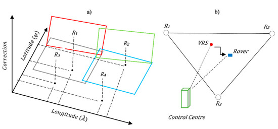
Figure 1.
(a) FKP method, (b) VRS method.
In the FKP method, the rover does not have to send its approximate position to the network solution centre. The FKP method creates plane correction parameters for east–west and north–south gradients (Figure 1a). These parameters are valid for a limited area around a master reference station. The rover then interpolates the model given the rover’s approximate position. For each reference station, a different model is constructed. In two-way communication the reference station closest to the rover location is designated as the master station, whereas in one-way communication the master station is selected by the user [9]. Another method commonly used in NRTK is the VRS correction model. As Figure 1b shows, a two-way line of communication is established in the VRS method, and the central CORS network software creates a virtual point close to the rover location. The precise positioning of the rover is established using the correction data obtained from the VRS point [10].
Both methods support concurrent data stream formats (RTCM 3.x). In VRS, a compatible tropospheric model is created through the virtual point; in FKP, there is a risk of incompatible tropospheric modelling between the rover and the reference station. In FKP, therefore, accuracy declines as the distance from the reference station increases. Similarly, this problem may also occur in the VRS method. However, it is easily resolved by re-initiating the rover after a certain distance. In this way, a new VRS point is created for the rover location. The server capacity of the control centre is more critical in VRS as a separate virtual point is created for each user, whereas the number of simultaneous users has a smaller effect on the server in the case of FKP [11].
In addition to the FKP and VRS correction methods, the Master-Auxiliary Concept (MAC) is also widely used, along with Master Auxiliary Corrections (MAX) and Individualized Master-Auxiliary Corrections (i-MAX). The MAC method works based on a master reference station and auxiliary reference stations. In this method, measurements performed by other auxiliary reference stations are sent to the master station. Observation and correction differences between stations are estimated. Accordingly, fit model parameters are sent from the master station to the rover. Instead of using network central software, with the fit model parameters sent by the master station, the software used in the rover determines the position error calculations [9,12]. Additionally, MAX and i-MAX methods have been developed using the MAC algorithm. MAX is based on the RTCM (3.1) network correction standard and provides master-auxiliary corrections for the entire network. For this method, bidirectional communication is not necessary with the server. For previous model receivers that do not interpret RTK (3.x), the i-MAX method was developed. In this method using real reference stations, corrections are transmitted in RTCM 2.3 and RTCM 3.0 formats. Unlike the MAX method, the i-MAX requires two-way communication [13].
Previous studies have used different scenarios to evaluate the performance of the correction models used in NRTK. Among these there have been studies investigating the performance of correction models in short time intervals (10 to 120 epochs) for stations with the same atmospheric conditions, regardless of baseline length [14,15]. In contrast, in studies examining the effects of satellite elevation angle and the number of measurement epochs on accuracy and precision, no significant differences were observed in elevation masks of up to 20 degrees, and a positive correlation was observed between the number of epochs and precision [16,17]. The effect of baseline length on accuracy and precision, on the other hand, continues to be investigated; several studies carried out in recent years have found no significant differences in solutions that use baseline lengths up to 40–50 km [18,19,20].
A review of current literature reveals the evaluation of correction models to be an active field of study. The present study examines the effect of baseline length on accuracy and precision in the case of the FKP and VRS correction models in particular and develops an empirical variance model as a function of baseline length. The CORS-TR network in Turkey was used for the NRTK model, while local stations in the ISKI CORS network were used as rovers. Three of the ISKI CORS stations selected as rovers were close to the CORS-TR stations, whereas the other three were relatively distant. Correlations between the accuracy and precision of the FKP and VRS correction models were analysed at different baseline lengths, and the variance model developed within this framework was tested using measurement values.
2. Study Area
The CORS-TR network, which was established in 2009 and has 158 stations, was used to broadcast the corrections. The area covered by the CORS-TR network contains six stations (ISTN, IZMT, KARB, SARY, SLEE, and TEKR). The local ISKI CORS network, established in Istanbul at the end of 2008, was used as the rover. A total of six stations were selected from the ISKI CORS network as rovers, three of them close to the CORS-TR stations (KCEK, SILE and TERK) and three further away (BEYK, SLVR and TUZL). Figure 2 shows the ISKI CORS and CORS-TR stations, as well as the CORS-TR interstation distances.
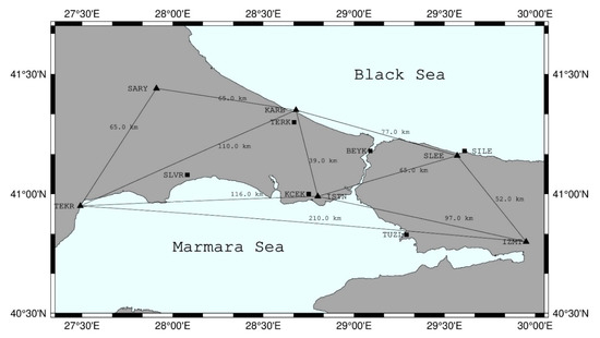
Figure 2.
ISKI CORS (rover) and CORS-TR (reference) stations in the study area (square icons represent ISKI CORS network stations; triangular icons represent CORS-TR network stations).
3. Static Survey Methodology
As explained in the previous section, although ISKI CORS stations are located within the CORS-TR network geometry, the two CORS networks operate independently. Network centres and their managements are different. While the datum of the ISKI CORS network is ITRF05 (2005.0 epoch), the datum of the CORS-TR network is ITRF96 (2005.0 epoch).
The CORS-TR network was used in NRTK correction broadcast (by choosing FKP and VRS methods). To test the NRTK survey, ISKI CORS stations were used as the rover, and their reference coordinates were determined in the ITRF14 datum (2005.0 epoch). The official coordinates of the ISKI CORS Network may be used as reference coordinate values, but the station coordinates have not been updated since its installation, and their velocities have not been determined (2008–2020). Instead of the ISKI CORS Network’s official coordinates, reference coordinate values were determined to investigate the consistency of the velocity values between stations.
Firstly, BERNESE (v5.2) (Astronomical Institute, University of Bern, Bern, Switzerland)software was used to determine the reference coordinates of the six stations selected as rovers, based on the seven IGS stations (ANKR, BUCU, CRAO, ISTA, NICO, SOFI, ZECK) and IGS products [21]. The locations of the IGS stations, which are the reference stations used in the static survey, are shown in Figure 3. IGS final orbit data were used in the evaluations made with reference to the ITRF14 datum and measurement epoch coordinates of the seven IGS stations [22]. Since the CORS-TR network used in NRTK correction broadcast produces ITRF96 (2005.0 epoch) coordinates, the velocity values were examined for determining the 2005 epoch coordinates of the six test points. To obtain reliable results in the velocity calculation of the test points, the observation dates were chosen as one day per month between 2008 and 2019, with a total of 129 sessions. The positional values identified were subjected to a time series analysis, and the linear trend statistic was calculated for the positional values at different epochs using the least-squares method. The positional values for the linear trend were defined as a function of measurement time. Additionally, 2005.0 epoch X, Y, and Z estimate (m) and annual trends (cm/year) were obtained for each station. The accuracy of the determined velocity values was tested. To test the compatibility of the velocity model statistically, R square values were examined for all stations along the X, Y, and Z axes. Accordingly, as seen in Table 1, the results were highly consistent (Mean R2 is 0.993). Thus, it was understood that there was no time-dependent station offset values (due to earthquakes, displacement, etc.) at the stations. Additionally, as CORS-TR stations are defined using the ITRF96 datum, the ITRF14 reference coordinate values of the rover stations were transformed into the ITRF96 datum with the ITRF online tool. The standard relation of transformation between the two reference systems is a Euclidian similarity of seven parameters: three translation components, one scale factor, and three rotation angles. Since the datum transformation parameters are fixed values, the tool is used for the transformation does not affect the results [23].
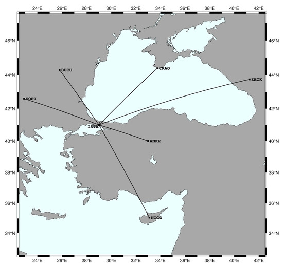
Figure 3.
IGS stations.

Table 1.
Reference coordinate values and velocities of the six test points.
4. NRTK Survey Methodology
RTKNAVI software was used for the FKP and VRS solutions due to its open-source code, and the fact that it permits NTRIP connections via a digital subscriber line (DSL). Measurements were made with 23,400 epochs (at 1-s intervals) between 10 pm and 4.30 am, with a one-day interval (26 October and 27 October 2019). An elevation mask of 15 degrees was used. The Saastamoinen model and Niell Mapping Function were used for troposphere delay. The measurements made for the KCEK, SILE, and TERK stations, which are closer to the CORS-TR stations, were made on the first day, with the measurements for BEYK, SLVR, and TUZL stations, which are further away, being made on the second day. The ISKI CORS network is an active network and since one station cannot be used as a reference and a rover, six stations were inactivated in the central software. To permit their use as rovers, the six stations were deactivated in the ISKI CORS network by removing them from the reference stations file in the Topnet-V software, which broadcasts corrections to the ISKI CORS network. A single RTK mountpoint was defined in the Topnet-V software for the six stations, making it possible to use them as rovers in the RTKNAVI software. The FKP and VRS solutions for the six stations were obtained in real-time through the corrections broadcast by the CORS-TR network, which uses Trimble CORS software. Figure 4 shows the working diagram of the system.
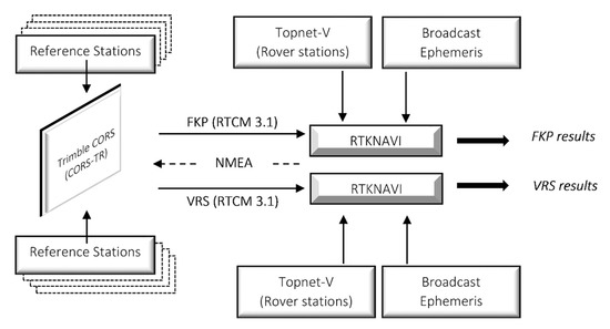
Figure 4.
Data communication diagram for FKP and VRS solutions.
For ambiguous solutions, all results were analysed at the FIX rate by filtering the FLOAT results. The Local Geodetic System (LGS) was used to evaluate the FKP and VRS solutions. To this end, the differences between the reference coordinates determined using BERNESE and the real-time NRTK solutions were transformed into LGS using Equation (1) [24].
Here, and are the topocentric and geocentric vectors, respectively. and is the geocentric to topocentric rotation matrix (as given within the curved brackets of Equation (2)).
Equation (2) shows the transformation vectors for the east, north, and upward axes in LGS (. represent the respective latitude and longitude values of the receiver position. After calculating the components of , RMSE and standard deviation values were calculated to estimate the accuracy and precision of the test points (Equation (3)). The correlation was analysed between the calculated RMSE and standard deviation values on the one hand and baseline length on the other.
In Equation (3), X expresses the reference coordinate values examined with the static survey, refers to coordinate values calculated with the NRTK survey, and is the average value of the NRTK coordinate values.
5. Variance Model Algorithm
For the NRTK survey we created a variance equation, predicting that the standard deviation values may be correlated with the root of the baseline lengths. The parameters for the mathematical equation between the standard deviation of NRTK measurements and baseline length were calculated experimentally; for this, Eckl’s experimental model was modified [25].
In Equation (4), the value expressed in terms of baseline length represents the standard deviation of measurements, represents measurement duration, and represents baseline length. , , c, and are constants of the models. Since a single measurement epoch (23,400 epochs for each test station) was used in the present study, the component was turned into a constant and removed from the equation. The rearranged equation, with the constants shown in parentheses, is as follows:
The solution to the observational equations and the normal equations for Equation (5) are expressed as follows:
In Equation (6), represents the coefficients of unknowns, represents the unknowns (), represents the standard deviations estimated from NRTK measurements, and represents the residuals. Based on the FKP and VRS measurements for the six rover stations, normal equations for the axes were written in the matrix form and solved (Equation (7)).
6. Results and Discussion
As outlined in the previous section, the reference coordinates of six test points from the ISKI CORS network were determined based on the IGS stations (Figure 2). Calculations were made using the academic BERNESE software, which can model distance-related errors in long baseline lengths. The more recent ITRF14 datum, which is assumed to provide more advanced solutions than previous datums, was preferred. Through time series analysis of the reference coordinates for 129 sessions, linear velocities were calculated and 2005 epoch fix coordinates were identified. As explained in the previous section, because the CORS-TR network that provides FKP and VRS solutions uses the ITRF96 datum, for consistency the reference coordinate values of the six test points were transformed into the ITRF96 datum. Table 1 reports the 2005 epoch reference coordinates and velocities of the six test points in the ITRF14 and ITRF96 datums. Additionally, in Table 1 the compatibility of the velocity model is shown with R2 statistical values.
The tectonic plate motion values and station velocities in Table 1 were compared to identify any stations that moved locally, independently of the network. The NUVEL1A model velocities for the area, in the directions X, Y, and Z, were −1.74 cm, +1.73 cm, and +0.77 cm per year, respectively. Analysis of the ITRF14 datum velocities in Table 1 showed that the TUZL station moved in the Y direction at a velocity that was 0.38 cm/year lower than the tectonic plate motion.
The six test points were divided into two groups based on their baseline lengths. FKP and VRS solutions were obtained simultaneously on two consecutive days. To be used as rovers, the six test points in the ISKI CORS network needed to be deactivated from the system. To minimise the disruption to users of the ISKI CORS network, which currently broadcasts corrections 24 h a day, measurements were made during night-time hours (10 pm–4:30 am).
Figure 5 shows the mean atmospheric activity of the stations along the zenith axis on two measurement days: these measurements were obtained using Topnet-V CORS software. These values were obtained in order to identify any differences between the tropospheric and ionospheric characteristics of the two measurement days. Figure 5a shows total zenith tropospheric delay values, and Figure 5b shows the Index I95h values for the measurement days, as an indicator of ionospheric activity. These observations show that the tropospheric and ionospheric activities on the two measurement days were approximately identical. An index value of 4, reported in Figure 5b, represents an average level of ionospheric activity, and an index value of 8 represents a high level of activity [26].
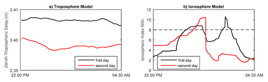
Figure 5.
Atmospheric corrections ((a) Troposphere Model, (b) Ionosphere model).
The CORS-TR control centre receives and processes the data of the reference stations in real time and sends the set of network products to the user via NTRIP in the RTCM format. In this study, CORS-TR network products were used to mitigate the impact of propagation errors from the ionosphere. Moreover, as measurements were made in real time, the broadcast data for satellite and clock ephemeris were used, and as the receivers in the ISKI CORS and CORS-TR stations allow the evaluation of GPS and GLONASS satellites only, no other satellites were included in the analysis. An uninterrupted 6.5 h of NRTK measurements were made over two consecutive days (23,400 epochs), and that created a suitable environment for satellite visibility and contributed to a low Geometric Dilution of Precision (GDOP) value.
For the six test points, reference coordinate values obtained through BERNESE and NRTK positional values obtained through RTKNAVI software were transformed into LGS coordinates using the transformation vector in Equation (1). The calculated LGS coordinate differences with respect to the reference coordinate values are shown in Figure 6 and Figure 7.
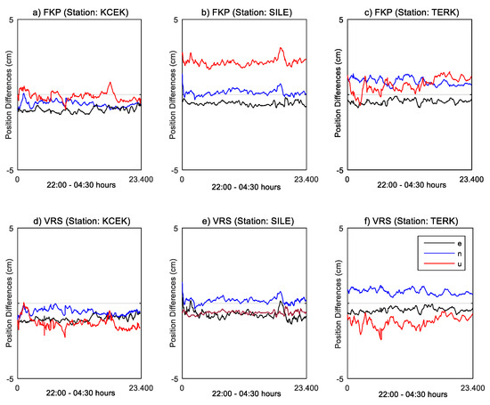
Figure 6.
The NRTK position differences at stations with a short baseline length ((a–c) are FKP results. (d–f) are VRS results).
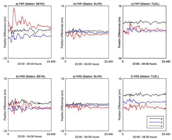
Figure 7.
The NRTK position differences at stations with a long baseline length ((a–c) are FKP results. (d–f) are VRS results).
The LGS coordinate differences for the FKP and VRS solutions of the KCEK, SILE, and TERK stations, which had short baseline lengths, are shown in Figure 6, and those of the BEYK, SLVR, and TUZL stations, which had long baseline lengths, are shown in Figure 7. Table 2 presents the RMSE and standard deviation values for the components of the FKP and VRS methods by baseline length. No significant linear correlation was determined between accuracy and baseline length. For the SLVR station, which had a long baseline length, the relatively low RMSE values of ±0.54 cm, 0.48 cm and 1.60 cm (mean values of the FKP and VRS methods) were calculated for the axes. The high RMSE value for the component for the TUZL station (mean: ±5.59 cm) can be attributed to the local movement along the Y-axis, as explained in the previous section.
Table 2.
RMSE and standard deviation values for the six test points.
The box graph in Figure 8 shows the error distributions according to the baseline lengths for FKP and VRS solutions. Red dots in the figure represent the outliers. Looking at the mean values, it is clear that the FKP and VRS methods generated results with similar levels of accuracy, which indicates that the accuracy achieved by the VRS and FKP methods does not differ significantly from baseline length. Considering the average of the differences in the axes, there are millimetric differences between FKP and VRS methods in the mean RMSE and standard deviation values, with calculations revealing a mean difference of 0.18 cm between RMSE values and 0.13 cm between standard deviation values.
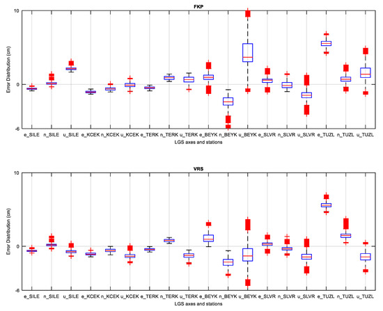
Figure 8.
FKP—VRS box plot.
An inspection of standard deviation values reported in Table 2 reveals a positive linear correlation with the baseline length. The correlation coefficients for the components are 0.80, 0.71, and 0.56 in the case of FKP (mean: 0.690), and 0.70, 0.78, and 0.60 in the case of VRS (mean: 0.693). As discussed in the previous section, we developed Equation (5) to strengthen this correlation. To calculate the coefficients (cm) and (cm/km0.5) in this equation, the matrix notations shown in Equation (7) were used. Table 3 shows the coefficients of the empirical model, obtained by the values given in Table 2.
Table 3.
Coefficients of the empirical model.
Figure 9 shows the standard deviations of the empirical model for the components derived from the FKP and VRS methods. Additionally, the dots indicated by the square symbol represent the standard deviation values examined from the NRTK measurements. As seen in Figure 9, for both methods there is a correlation of approximately 74.1% between the standard deviation values determined from the model and the measurements. Additionally, in order to observe the global variance of the performance of the model, the standard errors of the unit weight of the FKP and VRS models were estimated. Accordingly, the standard error of the unit weight of the models was estimated as ±0.11 cm, ±0.14 cm and ±0.44 cm along the respective axes. Additionally, the value of ±0.29 cm was estimated to express the standard error of the unit weight for all axes using the FKP and VRS methods.
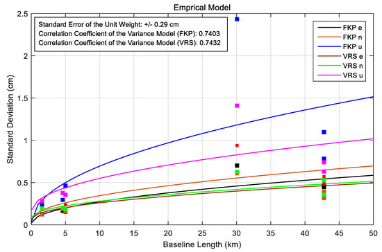
Figure 9.
Empirical variance models (FKP—VRS).
In Figure 10, there is a comparison of the linear model and the estimated variance model. The figure allows us to compare the compatibility of both models with the standard deviation values of the measurements. Accordingly, the nonlinear variance model defined by Equation (5) appears to better define the relationship between baseline length and standard deviation values (the linear model’s mean correlation is 69.2%, while the estimated variance model’s mean correlation is 74.1%).
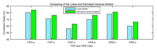
Figure 10.
Comparison of the Linear and Estimated Variance Models (FKP and VRS).
7. Conclusions
In the present study, we develop a new variance model after examining the effect of baseline length on accuracy and precision in NRTK measurements. ISKI CORS stations were used as rovers, and CORS-TR stations were used as references to test the variance model. NRTK measurements were made using the FKP and VRS correction models broadcast by the CORS-TR network. Various geodetic operations were performed for the study, including IGS-based positioning with long baseline lengths, datum transformation, and the transformation of coordinate differences into LGS. Moreover, various statistical calculations were undertaken, including velocity calculations of the identified coordinates through a time series analysis, and correlations of RMSE and the variance with baseline length.
The FKP and VRS methods were compared, and the differences were found to be at the scale of millimetres. In terms of accuracy, the RMSE difference between the two methods was 0.01 cm, 0.03 cm, and 0.57 cm for components respectively, and the standard deviation difference was 0.05 cm, 0.09 cm, and 0.25 cm. For baseline lengths of 1.6 km to 42.8 km, no significant correlation was found with positional accuracy. However, a mean linear correlation of 69.2% was found with precision. Based on this observation, a variance model was developed for precision by modifying the accuracy model of Eckl et al. [25]. In this context, (cm) and (cm/km0.5) variance model unknowns were defined for the FKP and VRS methods. For the test of the developed model, the standard error of the unit weight of the model and the correlation coefficients were determined. It was understood that the results were better than those using the linear model (mean correlation is 74.1%).
Further analyses showed that the movement of the TUZL station along the Y-axis varied from that of the ISKI CORS network by 0.38 cm in IGS-based positioning. The positional values of the TUZL station, which moves locally, should be updated on a periodical basis, and the reference coordinate values used in the ISKI CORS network should be redefined as needed.
Author Contributions
Investigation, Ö.G. and M.T.Ö.; Methodology, Ö.G.; Software, Ö.G.; Supervision, M.T.Ö.; Validation, M.T.Ö.; Visualization, Ö.G.; Writing—original draft, Ö.G.; Writing—review & editing, M.T.Ö. All authors have read and agreed to the published version of the manuscript.
Funding
This research received no external funding.
Acknowledgments
Firstly, the authors thank the International GNSS Service (IGS) for providing open access to high-quality GNSS data products. Secondly, the authors would like to thank the Istanbul Water and Sewerage Administration for providing full access to ISKI CORS network data and Topnet-V software. Also, the authors thank everyone who created the RTKLIB software and enabled open-source development.
Conflicts of Interest
The authors declare no conflict of interest.
References
- Edwards, S.J.; Cross, P.A.; Barnes, J.B.; Betaille, D. A methodology for benchmarking real-time kinematic GPS. Surv. Rev. 1999, 35, 163–174. [Google Scholar] [CrossRef]
- Colombo, O.L.; Hernández-Pajares, M.; Juan, J.M.; Sanz, J.; Talaya, J. Resolving Carrier-Phase Ambiguities on the Fly, at More than 100 km from Nearest Reference Site, with the Help of Ionospheric Tomography. In Proceedings of the 12th International Technical Meeting of the Satellite Division of the Institute of Navigation (ION GPS 1999), Nashville, TN, USA, 14–17 September 1999; pp. 1635–1642. Available online: https://www.ion.org/publications/abstract.cfm?articleID=3312 (accessed on 15 December 2019).
- Gao, Y.; Li, Z.; McLellan, J.F. Carrier Phase Based Regional Area Differential GPS for Decimeter-Level Positioning and Navigation. In Proceedings of the 10th International Technical Meeting of the Satellite Division of the Institute of Navigation (ION GPS 1997), Kansas City, MO, USA, 16–19 September 1997; pp. 1305–1313. Available online: https://www.ion.org/publications/abstract.cfm?articleID=2916 (accessed on 15 December 2019).
- Han, S. Carrier Phase-Based Long-Range GPS Kinematic Positioning. Ph.D. Thesis, School of Geomatic Engineering, The University of New South Wales, Sydney, NSW, Australia, 1997. Available online: https://ci.nii.ac.jp/naid/10006711990/ (accessed on 15 December 2019).
- Hu, G.R.; Khoo, H.S.; Goh, P.C.; Law, C.L. Development and assessment of GPS virtual reference stations for RTK positioning. J. Geod. 2003, 77, 292–302. [Google Scholar] [CrossRef]
- Lachapelle, G.; Alves, P.; Fortes, L.P.; Cannon, M.E.; Townsend, B. DGPS RTK positioning using a reference network. In Proceedings of the 13th International Technical Meeting of the Satellite Division of the Institute of Navigation (ION GPS 2000), Salt Lake City, UT, USA, 19–22 September 2000; pp. 1165–1171. Available online: https://www.ion.org/publications/abstract.cfm?articleID=1518 (accessed on 15 December 2019).
- Odijk, D.; Marel, H.V.D.; Song, I. Precise GPS Positioning by Applying Ionospheric Corrections from an Active Control Network. GPS Solut. 2000, 3, 49–57. [Google Scholar] [CrossRef]
- Koivula, H.; Kuokkanen, J.; Marila, S.; Lahtinen, S.; Mattila, T. Assessment of sparse GNSS network for network RTK. J. Geod. Sci. 2018, 8, 136–144. [Google Scholar] [CrossRef]
- Park, B.; Kee, C. The Compact Network RTK Method: An Effective Solution to Reduce GNSS Temporal and Spatial Decorrelation Error. J. Navig. 2010, 63, 343–362. [Google Scholar] [CrossRef]
- Wanninger, L. The Performance of Virtual Reference Stations in Active Geodetic GPS-networks under Solar Maximum Conditions. In Proceedings of the 12th International Technical Meeting of the Satellite Division of the Institute of Navigation (ION GPS 1999), Nashville, TN, USA, 14–17 September 1999; pp. 1419–1428. Available online: https://www.ion.org/publications/abstract.cfm?articleID=3291 (accessed on 15 December 2019).
- CORS-TR. Available online: https://tkgm.gov.tr/tr/icerik/tusaga-aktif-sistemi-duzeltme-parametreleri (accessed on 15 December 2019).
- Öğütcü, S.; Kalayci, S. Investigation network-based RTK techniques: A case study In urban area. Arab. J. Geosci. 2016, 9, 199. [Google Scholar] [CrossRef]
- Garrido, S.M.; Giménez, E.; de Lacy, C.M.; Gil, A.J. Testing precise positioning using RTK and NRTK corrections provided by MAC and VRS approaches in SE Spain. J. Spat. Sci. 2011, 56, 168–184. [Google Scholar] [CrossRef]
- Berber, M.; Arslan, N. Network RTK: A case study in Florida. Measurement 2013, 46, 2798–2806. [Google Scholar] [CrossRef]
- Gumus, K.; Celik, C.T.; Erkaya, H. Investigation of accurate method in 3-D position using CORS-net in Istanbul. Bol. Ciênc. Geod. 2012, 18, 171–184. [Google Scholar] [CrossRef][Green Version]
- Gumus, K. A research on the effect of different measuring configurations in Network RTK applications. Measurement 2016, 78, 334–343. [Google Scholar] [CrossRef]
- Gumus, K.; Selbesoglu, M.O.; Celik, C.T. Accuracy investigation of height obtained from Classical and Network RTK with ANOVA test. Measurement 2016, 90, 135–143. [Google Scholar] [CrossRef]
- Baybura, T.; Tiryakioglu, İ.; Ugur, M.A.; Solak, H.İ.; Safak, S. Examining the Accuracy of Network RTK and Long Base RTK Methods with Repetitive Measurements. J. Sens. 2019. [Google Scholar] [CrossRef]
- Ogutcu, S. Temporal Correlation length of network rtk techniques. Measurement 2019, 134, 539–547. [Google Scholar] [CrossRef]
- Ogutcu, S.; Kalayci, I. Accuracy and precision of network-based RTK techniques as a function of baseline distance and occupation time. Arab. J. Geosci. 2018, 11, 354. [Google Scholar] [CrossRef]
- Dach, R.; Lutz, S.; Walser, P.; Fridez, P. (Eds.) Bernese GNSS Software Version 5.2. User Manual; Astronomical Institute, University of Bern, Bern Open Publishing: Bern, Switzerland, 2015; ISBN 978-3-906813-05-9. [Google Scholar] [CrossRef]
- Dow, J.M.; Neilan, R.E.; Rizos, C. The International GNSS Service in a changing landscape of Global Navigation Satellite Systems. J. Geod. 2009, 83, 191–198. [Google Scholar] [CrossRef]
- ITRF. Available online: http://www.epncb.oma.be/_productsservices/coord_trans/index.php (accessed on 15 December 2019).
- Leick, A. GPS Satellite Surveying; John Willey & Sons Inc.: Hoboken, NJ, USA, 1995. [Google Scholar]
- Eckl, M.C.; Snay, R.A.; Soler, T.; Cline, M.W.; Mader, G.L. Accuracy of GPS-derived relative positions as a function of interstation distance and observing-session duration. J. Geod. 2001, 75, 633–640. [Google Scholar] [CrossRef]
- Gianniou, M.; Mitropoulou, E. Impact of high ionospheric activity on GPS surveying: Experiences from the Hellenic RTK-network during 2011–12. In Proceedings of the EUREF Annual Symposium, Saint Mandé, France, 6–8 June 2012. [Google Scholar]


© 2020 by the authors. Licensee MDPI, Basel, Switzerland. This article is an open access article distributed under the terms and conditions of the Creative Commons Attribution (CC BY) license (http://creativecommons.org/licenses/by/4.0/).