


Abstract
We study photon scattering in a transparent dispersive medium around a spherical geometry whose lapse contains independent inverse-radius terms through the fifth order. Free millicharged particles and neutral dark atoms provide microscopic response models through cold-plasma dispersion and dynamical polarizability, respectively. A joint expansion to the second order in the metric and susceptibility amplitudes retains every pairwise gravitational contribution and every mixed term coupling gravity and dispersion. The mixed coefficients depend on the logarithmic frequency derivative of the response. We separately derive a complete expansion through the fifth order in the inverse impact parameter using a generating formula that retains all nonlinear contributions at each radial order. Explicit vacuum coefficients and coefficients for a medium with an inverse-radius susceptibility relate the two expansions while preserving their distinct order counting. For an inverse-radius susceptibility, a relation between the leading radial coefficients and their spectral variation isolates the inverse-square metric coefficient under specified material assumptions. Higher metric coefficients require additional radial information and control of nonlinear material response. Calculations using exact rays test the expansions, reproduce the coefficient bias from neglected refraction, and quantify the conditioning of frequency subtraction. The metric is a phenomenological exterior ansatz. The calculation provides a consistent framework for separating geometric and material contributions in weak dispersive lensing.
1. Introduction
Weak gravitational lensing measures the geometry sampled by a ray only after its propagation through matter has been specified. A dispersive medium changes both the ray trajectory and the frequency dependence of its bending. Therefore, the relevant inverse problem is not simply whether the angle increases or decreases when a metric parameter is varied. It is whether a coefficient attributed to geometry can instead arise from refraction at the same radial order. This question already occurs for a spherical lapse containing mass and inverse-square terms, without choosing a particular gravitational field theory.
The distinction between a bending law and gravitational lensing is important even in a vacuum. Studies of naked-singularity lenses, time delays and magnification centroids, and relativistic Schwarzschild images show how different aspects of the lens map carry information about a compact object [1,2,3]. Image distortions and proposed conservation relations for distortion provide further characterizations of that map [4,5]. The present work addresses an earlier step in such an inference: separating geometric and material contributions to the scattering angle before constructing image positions, magnifications, or arrival-time differences.
The geometric ingredients of the optical approach, including curvature, geodesic curvature, and the Gauss–Bonnet theorem, belong to the standard framework of differential geometry [6,7]. Gibbons and Werner applied that theorem to express asymptotic gravitational bending as an integral of optical Gaussian curvature [8]. Werner extended the construction to Kerr–Randers optical geometry [9], while finite-distance formulations treated static configurations in weak and strong deflection and stationary axisymmetric geometries [10,11,12]. These developments distinguish the curvature contribution from the local angles and boundary terms required by a specified observer configuration.
That distinction becomes particularly important without an asymptotically flat reference region. Work on Schwarzschild–de Sitter bending and the projective properties of its optical metric separates questions about unparametrized trajectories from questions about measured angles [13,14]. Definitions based on total deflection or observer geometry further clarify the role of the reference construction [15,16]; corrections from the cosmological constant to the photon sphere and shadow radii concern related but distinct quantities [17]. We restrict the calculation below to asymptotically flat scattering, rather than identifying its asymptotic bending angle with every finite-distance or shadow observable.
Several reductions make the curvature formulation practical. Its equivalence with the geodesic approach was examined by Li and Zhou [18], and boundary constructions based on circular orbits were developed by Li, Zhang, and Övgün [19]. Boundary expressions in isothermal coordinates, radial integral reformulations, and reference-renormalized curvature primitives offer complementary ways of organizing finite-distance calculations [20,21,22]. The extension to spinning massive particles illustrates why a non-geodesic physical boundary requires its own contribution from geodesic curvature [23]; intrinsic particle spin is not included here. For the dispersive photon problem, the relevant higher-order issue is that expanding the optical curvature alone is insufficient: the ray bounding the integration domain must also be displaced consistently.
Strong deflection provides a useful contrast to this expansion for weak scattering. Photon surfaces supply the geometric description of trapped null trajectories [24], and the usual expansion for strong deflection is controlled by the approach to an unstable photon sphere [25,26]. Marginally unstable and degenerate photon spheres require different asymptotic treatments, including the configurations studied by Tsukamoto and Sasaki [27,28], the expansion of Igata, Sasaki, and Tsukamoto [29], and trajectories approaching from inside and outside a marginal sphere [30]. A formulation in terms of local geometric invariants and matter distributions further clarifies the coefficients of strong deflection [31]. These results delimit, rather than extend, the regime of our series in the inverse impact parameter; the weak law is not continued through the capture threshold.
Other observables of compact objects involve additional dynamical information. Relations between the instability of null orbits, eikonal quasinormal frequencies, and strong lensing were developed in [32,33]. Joint studies of optical and wave quantities include dyonic ModMax black holes and a first-order eikonal treatment of a scalarized metric [34,35]. The energy dependence of massive-particle shadows and redshift spectroscopy provide other routes to investigate geometric parameters [36,37]. These are neighboring inference problems, not observables calculated in this paper. In particular, a photon bending law alone is not a determination of the coupled gravitational perturbation spectrum.
The Hamiltonian description of rays in refractive media provides the propagation framework [38,39]. Nonuniform plasma lensing contains contributions from both gravity and refractive gradients [40]. The Gauss–Bonnet treatment of plasma rays and their correspondence with massive-particle scattering were developed in [41]; curvature and energy-momentum formulations were subsequently extended to dispersive propagation [42]. Higher-order plasma bending is not new: Crisnejo, Gallo, and Jusufi included higher-order corrections and nonhomogeneous plasma [43], while Comberiati and de la Cruz obtained next-to-leading purely refractive terms for power-law profiles using worldlines [44]. General spherical dispersive propagation was treated by Tsupko [45]. These studies, rather than leading-order metric substitutions alone, provide the comparison for the joint expansion below.
Material effects also enter the shadow problem in spherical geometries and separable plasma configurations on Kerr spacetime [46,47]. Deflection in moving media requires a specified material velocity field [48], and calculations for dusty plasma explicitly address both dispersion and absorption [49]. Our approximation of a static, transparent medium excludes those additional effects unless they are incorporated into a new propagation model. Model-dependent applications include particle dynamics and weak lensing in Kalb–Ramond gravity [50], deflection and energy conditions for wormholes in extended teleparallel gravity [51], and the effects of plasma on deflection and shadows of charged torus-like black holes [52]. Their differing source geometries and material assumptions should not be identified with the spherical scattering problem considered here.
Dark-sector examples require a further distinction between changing the spacetime through gravitating matter and changing photon propagation through an electromagnetic response. Kinetic mixing supplies a possible origin for small effective electric charges [53]. A cosmic refractive index and matter-induced dispersion at cosmological distances have been examined as probes of such interactions [54,55], and phenomenological refractive effects of dark matter have also been studied using the Gauss–Bonnet method [56]. Here, a dark-sector species is an illustrative candidate for a response function, not an assumption that ordinary photons interact with every form of dark matter.
Models of atomic dark matter distinguish free charged constituents from neutral bound states [57,58]. Astrophysical constraints on millicharged atoms and the optical dispersion of composite particles motivate the separate free-particle and polarizability examples used below [59,60]. Their physical parameter space is also subject to cosmological constraints and collective plasma effects [61,62]. The LUX-ZEPLIN constraint on atmospherically produced millicharged particles supplies an experimental example, but it is not a direct measurement of a refractive halo around a black hole [63]. No illustrative susceptibility amplitude in this work is inferred from that experiment. Free cold, charged species enter our model through the sum of their squared plasma frequencies, whereas atomic polarizability can become nearly achromatic or absorptive; these are restrictions on inference, not evidence of detection.
Millicharged matter provides a concrete motivation for treating the geometry and optical response together. Its refractive strength depends on charge, mass, abundance, and ionization state, while neutral composites introduce an internal excitation scale. A common scattering calculation can therefore compare responses with the same prescribed exterior and trace their microscopic parameters into the frequency dependence of the bending coefficients. This is useful when testing whether a putative metric correction could instead reflect an incompletely modeled material contribution. We develop the free-particle and atomic examples explicitly, including the gravitational shift of their local response, so that the phenomenological susceptibility can be interpreted within a specified particle model.
General high-order metric expansions are established tools [64]. We give both orderings explicitly, with a coefficient generator for the complete radial series. For an inverse-radius medium, this generator retains the nonlinear material terms that can otherwise be mistaken for higher metric coefficients.
Our main application is coefficient inference. For an inverse-radius susceptibility, the leading chromatic coefficient determines the material contamination of the inverse-square bending coefficient through a frequency derivative. We test that relation with exact rays in a metric containing all four deformation coefficients, and identify its sensitivity to a separate response quadratic on density. Plasma subtraction using three frequencies tests the quadratic spectral model; the complete fifth-order radial plasma polynomial generally requires six bands. The corresponding null relations test the retained spectral form at a common impact parameter. The higher radial coefficients are organized by a triangular series, whose practical use depends on response information and numerical conditioning. The results concern a prescribed exterior geometry and transparent scattering.
2. A Generic Spherical Exterior
2.1. Metric Expansion and Its Motivation
We consider the static, asymptotically flat line element
with signature and . The radial coordinate is the areal radius, is the asymptotic mass, and
The coefficients are independent signed parameters. The symbol b is reserved for the coefficient of ; throughout the optical calculation, the asymptotic impact parameter is denoted by B. Photons couple minimally to the displayed metric.
Equation (1) is a finite phenomenological expansion of a spherical exterior. It resolves departures from the mass term into successive radial orders and makes it possible to examine which geometric contributions can be separated from refraction. In a vacuum, the leading effects of and d enter the bending angle at orders and , respectively. Nonlinear gravitational terms and mixed material terms can contribute at these same orders. Their radial scaling alone therefore does not determine a metric coefficient.
No source action or gravitational field equation is imposed. In particular, a fitted coefficient is not assigned a charge or a microscopic interpretation. The condition in areal-radius coordinates is part of the ansatz: a fully general static spherical exterior contains two independent radial metric functions. The present parametrization supplies a controlled setting for optical inference within that restriction.
Two uses of the ansatz should be distinguished. If Equation (1) is prescribed exactly over the exterior region, its horizons and circular null orbits can be determined from the equations below. If it is regarded only as the first five inverse-radius terms of an asymptotic expansion, predictions near a candidate horizon also depend on the omitted terms. The weak-scattering expansion is governed by
with the corresponding conditions holding along the accepted ray. An omitted metric term of order first affects vacuum bending at an order , provided the ray remains within the asymptotic domain.
2.2. Exterior Region and Vacuum Circular Rays
A positive Killing-horizon radius solves
When such a root exists, the exterior connected to spatial infinity is selected by ; its inner boundary is the largest positive root . The coefficients need not produce a horizon, and may give multiple or degenerate roots. Thus, a parameter choice must be checked before the ansatz is described as a black-hole exterior. When the physical lens has a material surface, that surface supplies the inner boundary instead.
For vacuum equatorial null geodesics, the effective potential per unit squared angular momentum is
Circular null orbits satisfy , or, equivalently,
Only positive roots in the chosen static exterior are relevant. A local maximum of is unstable, a local minimum is stable, and a root with requires a higher-order classification. Each exterior unstable root has the associated vacuum impact parameter
There can be more than one exterior extremum, so selecting a root by its radius alone does not determine capture. For an absorbing black-hole horizon, the vacuum threshold is fixed by the highest exterior barrier,
An escaping ray turns at the outermost root of accessible from infinity. These conditions refer to vacuum null propagation. A dispersive medium changes both the turning-point and circular-ray conditions.
The curvature can be evaluated without assigning a source theory. For the metric in Equation (1),
In particular, the higher inverse-radius terms need not preserve the vanishing Ricci scalar of the subfamily containing only the mass and inverse-square terms. Compact expressions for two further invariants are
For finite coefficients, these invariants are finite at every positive regular root of f; the coordinate singularity there can be removed using an ingoing null coordinate. The inverse-radius ansatz is generally singular at , outside its intended exterior domain. These geometric facts alone do not determine the dynamical stability or matter content of a gravitational theory.
For interpretation within Einstein gravity only, one could define , which gives , , and . This is an effective reconstruction from the specified geometry; it imposes no material model on the ray calculation.
The millicharged populations introduced below are prescribed as test media. Their densities are independent of and d in this calculation. Using the same population to source the exterior would additionally require its stress tensor, a consistent equilibrium or flow model, and gravitational backreaction. The present separation isolates how an electromagnetic response changes photon propagation through a specified geometry.
3. Material Response and Local Frequency
The material examples connect a prescribed refractive response to microscopic properties of a possible dark component. Free charges respond collectively, whereas a neutral atom responds through its internal electric dipole transitions. The binding interaction and the coupling to ordinary light are distinct: the dark fine-structure constant determines the atomic spectrum, while the ordinary millicharge controls the strength of its electromagnetic response [57,58,60]. These examples provide physically specified choices for the susceptibility used in the scattering calculation.
For a static medium, the four-velocity is . The conserved Killing frequency and the local rest-frame frequency obey [41]
Every microscopic response below is evaluated at this local frequency. Number densities are proper densities measured in the material rest frame. We use Gaussian electromagnetic units, with when , and neglect magnetic response.
3.1. Free Millicharged Dark Particles
Let X be a nonrelativistic dark particle with a mass and ordinary electric charge
Here, denotes its rest-mass density. A small ordinary charge can arise from kinetic mixing with an unbroken dark gauge field [53]. We adopt the realization with a massless dark photon and a constant effective ordinary charge; a massive mediator can require a different electromagnetic response [60].
In the cold, isotropic, nonmagnetized approximation, the species contributes
Consequently, in the generic exterior of Equation (1),
This expression retains all five inverse-radius contributions to the lapse. Propagation requires along the entire ray, and the weak expansion additionally requires the susceptibility to be small there. The response is proportional to ; a small charge alone therefore does not determine its size without a mass and density model [54,55].
For several cold charged species, including ordinary plasma and unbound dark constituents, the squares of their plasma frequencies add. Opposite charge signs do not cancel this response. A quasi-neutral population or an explicit neutralizing component is assumed, so that a background electric field is not implicitly introduced into the prescribed geometry. Species with the same total plasma-frequency field produce the same rays in the adopted Hamiltonian. Thus, a measurement of its amplitude constrains a combination of microscopic parameters and cannot by itself identify a dark species. Finite velocity dispersion, anisotropy, magnetic fields, or appreciable collisional damping require the corresponding dielectric response; a cold collisionless population is already included in the present limit.
For a power-law profile, define
The reference radius specifies the density normalization. The dimensionless response normalization at the conserved frequency is ; the local susceptibility also includes the density profile and the frequency shift in Equation (14). For , the susceptibility vanishes at infinity. The power law supplies an analytic model over the scattering region; a physical halo also requires the finite extent and dynamical conditions discussed in Section 9.
3.2. Millicharged Atomic Dark Matter
Atomic dark matter consists of oppositely charged constituents bound by a dark electromagnetic interaction [57,58,61]. In the kinetic-mixing realization considered here, constituents of masses and carry ordinary charges and . The bound state is neutral under ordinary electromagnetism but acquires an induced electric dipole moment in an applied field. This distinguishes its response from that of its unbound constituents [59,60].
At leading order in the density of a dilute isotropic gas of ground-state atoms, the complex refractive index is represented by
The dynamical electric polarizability relates the induced dipole moment to the ordinary electric field. Here, are dimensionless oscillator strengths for the isotropic response, are electric-dipole transition frequencies, and are damping widths. With time dependence , the displayed denominator gives positive absorption for positive oscillator strengths. For a narrow isolated line, is the leading absorptive full width at half maximum; a convention based on the amplitude decay rate differs by a factor of two. The strengths must include the angular averages and level degeneracies appropriate to the microscopic model [60]. A finite oscillator sum is an effective description of a chosen spectral window; a complete atomic polarizability also includes continuum states.
For a nonrelativistic Coulomb potential , where is the internal constituent separation and is the dark fine-structure constant, the bound energies and first electric-dipole excitation obey
This is the leading scale, without a fine or hyperfine structure. The ordinary millicharge suppresses the response amplitude in Equation (21), while and set the resonance location.
In the curved exterior, the atomic response becomes
For , define the real susceptibility amplitude
The real optical calculation uses this amplitude in a transparent spectral window. It also requires small absorption over the full path, including the gravitational change of local frequency. The effect of the discarded imaginary part at the second material order is specified in Section 9.
A single oscillator contribution has
Its sign changes across the line; the sign of a sum over transitions depends on all contributions. Well below the lowest electric-dipole resonance and for weak damping, the polarizability of the ground-state model is positive and nearly independent of frequency. In the lossless single-line approximation,
This illustrates how the almost constant response at low frequency develops appreciable dispersion as the excitation scale is approached. Near resonance, absorption and large spectral derivatives invalidate the assumed transparent weak expansion. The real Riemannian optical metric is therefore applied only within an accepted transparency window.
3.3. Connection to the Scattering Response
We write both examples as a separable weak response:
If free constituents and neutral atoms share this radial power, their dilute susceptibilities add, giving . Only unbound charges enter ; bound constituents are already represented by the atomic polarizability. Distinct radial profiles require a sum of response terms, with corresponding changes to the inference relations derived for one profile. The ionization fraction thus affects both the amplitude and the spectral form of the material contribution.
To connect Equation (27) with the weak-index expressions, set
Under the joint scaling and , with controlled spectral derivatives, the positive real index is
The first correction is for free particles and for atoms. The mixed term contains every coefficient in and the logarithmic frequency derivative of the microscopic response. It is retained in the bending calculation, together with the displacement of the ray.
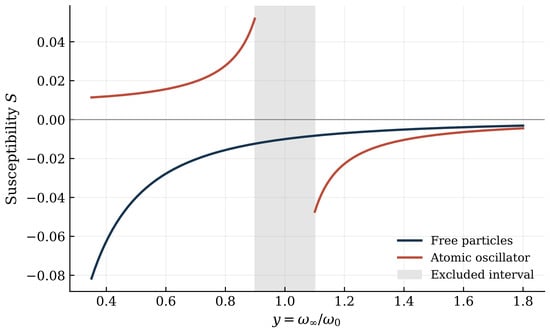
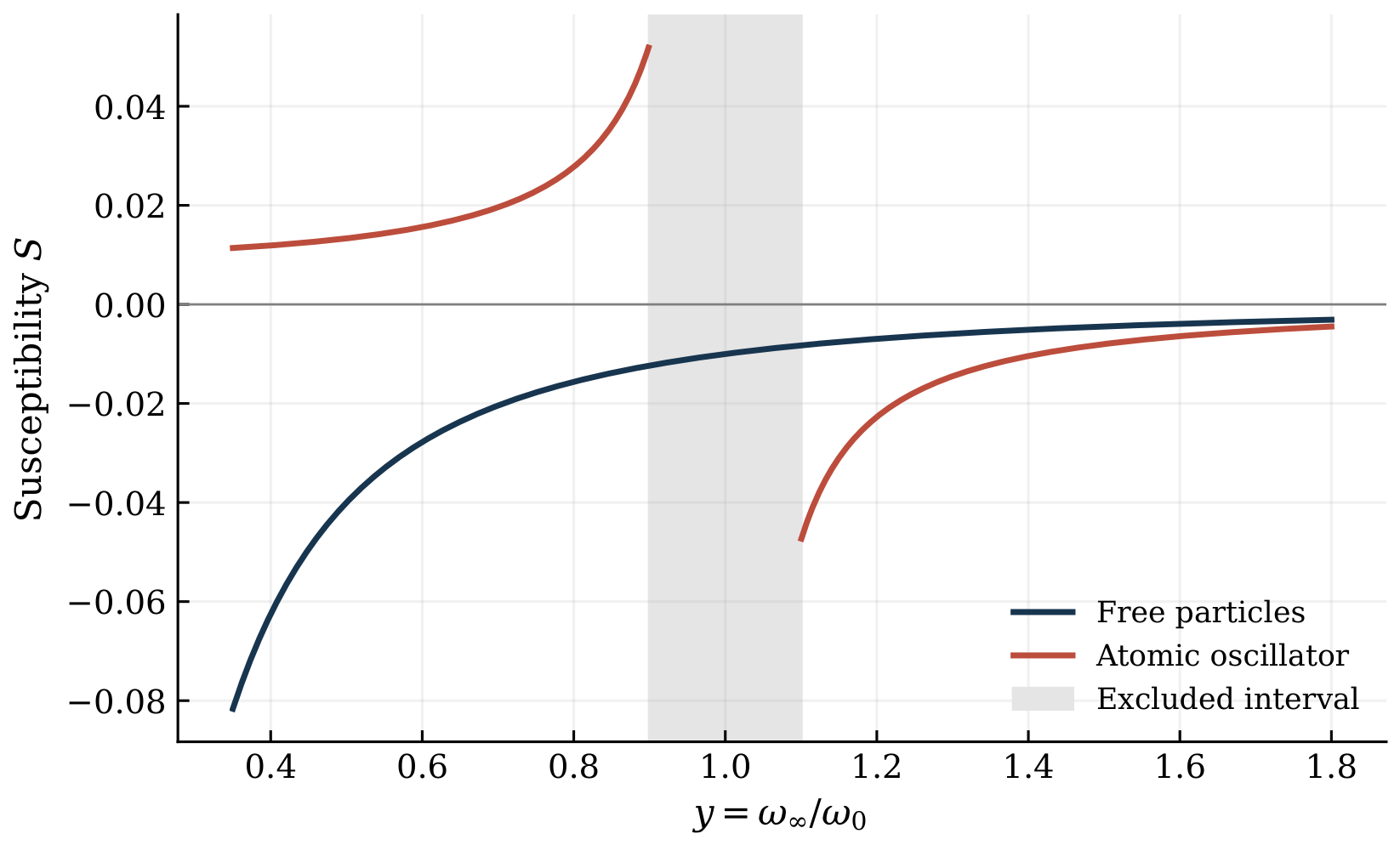
Equation (27) specifies an index model linear in density. Iterating its rays to a higher order does not add microscopic response coefficients quadratic in density. This distinction is relevant when the material susceptibility is used to infer geometric coefficients at the same radial order. Figure 1 compares the frequency dependence of the free millicharged-particle and neutral atomic responses evaluated at the asymptotic frequency. The atomic response changes sign across the resonance, whereas the free-particle response remains negative and scales as .
Figure 1.
Illustrative asymptotic responses: and , where . The plotted exclusion is illustrative; ray acceptance also checks the gravitationally shifted frequency. This plot of the material response is independent of the metric coefficients.
4. Exact Rays and Optical Curvature
The Hamiltonian of an isotropic dispersive medium is [38,39,45]
In the static spherical setting, and are conserved. For cold plasma, the material term is , so equal total plasma-frequency profiles give exactly identical Hamiltonians and rays.
At a fixed frequency, the equatorial spatial trajectories are geodesics of
This spatial optical line element is distinct from group travel time in a dispersive medium. The latter also involves frequency derivatives of the response.
For the diagonal radial optical metric, the curvature two-form is an exact derivative:
The radial derivative includes the local-frequency dependence in Equation (14). For a simple scattering ray and an asymptotic region with , the Gauss–Bonnet relation is
A higher-order calculation must consistently account for the displaced boundary and its angular interval.
Let , and define
Then, and the exact radial equation is
The scattering turning point is the first positive simple zero reached from through to , , and . The same domain must remain free of material poles. This selection replaces any closed turning-radius formula specific to a lower-order lapse.
A useful alternative variable is the normalized optical impact radius,
On an exterior monotone scattering branch,
The turning point is now fixed at . This expression gives both expansions below and supplies a direct link between the exact ray integral and optical geometry.
5. A Complete Second-Order Amplitude Expansion
5.1. Ordering and General Power-Law Response
For , the index tends to one at infinity. Define the signed susceptibility amplitudes
We count every in Equation (34) and the full susceptibility function as the first order:
Spectral derivatives scale with the same susceptibility amplitude. This differs from assigning the order ; the coefficients are independent here. Define the angular moments
For all positive exponents appearing below, these are finite.
The complete degree-two result is
The derivation of Equation (41) and the corresponding homogeneous-response kernel is presented in Appendix A. The double sum is ordered: each off-diagonal product occurs twice. The linear terms in the metric amplitudes begin as
Equation (41) includes all quadratic products in the metric amplitudes, all five mixed contributions coupling the metric and the response, and iteration of the refractive trajectory. For a local power response, , the coefficient multiplying is
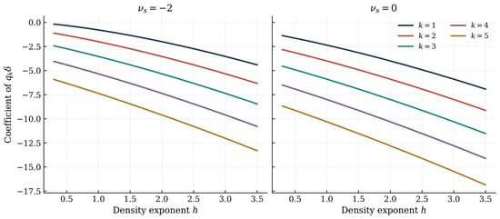
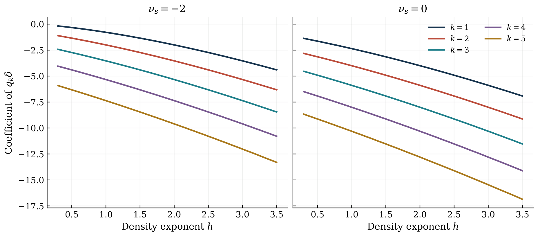
Since , its contribution coupling mass and response has the familiar positive prefactor multiplying . The signs of the higher metric contributions depend independently on and d, and on the response. Figure 2 compares the mixed coefficients for all five metric powers, showing how they depend on the density exponent h for cold-plasma dispersion () and a locally constant response (). The sign of each contribution to the bending angle also depends on the signed product .
Figure 2.
Mixed coefficients for each metric power , with cold-plasma slope and locally constant response . The coefficient multiplies the signed product ; its plotted sign alone is not the sign of the angle correction.
In cold plasma, , giving
Taking only the mass in the mixed term recovers the established and plasma contributions [43]:
The general purely refractive quadratic coefficient agrees with [44]. These limits are checks of the generalized response law.
For free millicharged matter, Equations (44) and (45) use the same spectral law as ordinary cold plasma, with the microscopic normalization in Equation (16). For a density decreasing outward, the leading gradient contribution is outward because . Below the first atomic excitation, instead gives an inward leading refractive contribution. The atomic logarithmic slope in Equation (26) also changes the mixed coefficients in Equation (43). These signs describe the leading material terms; the total bending includes gravity and all retained mixed contributions.
The remainder in Equation (41) contains all amplitude degrees of at least three. Terms quadratic in the metric amplitudes can scale as , while omitted terms cubic in mass already scale as . Thus, this is not a complete fifth-order inverse-impact expansion. Section 6 constructs that distinct expansion. For noninteger h, the general amplitude formula remains applicable without assuming an ordinary Taylor series in .
5.2. A Homogeneous Dispersive Response
A homogeneous medium has in general. Define
Normalizing the optical impact radius by gives
A constant normalization of n drops out, while frequency derivatives remain because gravity changes the local frequency. The first mass term agrees with [45]. The cold-plasma and general-metric expansions connect with [43,65].
For constant plasma frequency,
The square bracket in Equation (47) becomes . The exact radial function is
Weak bending close to a cutoff requires the velocity-enhanced perturbations to remain small. Large alone does not ensure that condition as . Setting in a decaying-medium formula would miss the change in , and is not used here.
6. Complete Radial Expansion Through the Fifth Order
At fixed dimensional coefficients, write , , and , with . For a response admitting a Taylor expansion at infinity, the exact construction using the optical impact radius gives
Here, denotes coefficient extraction. To see this, set and define . The angular kernel is . Lagrange inversion gives
Integrating each monomial yields the factor . The constant term contributes and cancels from the deflection angle. High-order deflection using inverse series is established [64,65]; the response factors in Equation (50) make the material bookkeeping explicit. For noninteger density powers, fractional radial powers generally occur, and Equation (41) supplies the separate general-h amplitude result.
6.1. Complete Vacuum Expansion Through the Fifth Inverse Power of the Impact Parameter
The inverse-radius hierarchy supplies a check independent of any expansion in independent deformation amplitudes. At fixed and d, the complete vacuum law through is
where
All nonlinear products allowed at each inverse-impact order are retained. For example, the and terms cannot be omitted from a complete large-B expansion while the term is kept. A separate expansion through the second degree in independent amplitudes has a different ordering, and should be identified explicitly as such.
6.2. Complete Coefficients for an Inverse-Radius Medium
For , the index tends to unity at infinity. Define
Equation (50) applies at fixed dimensional metric coefficients and fixed smooth response. It retains every material and gravitational product contributing through within the assigned linear index law. It requires a transparent escaping ray and controlled spectral derivatives over the redshifted frequency interval. For explicit expressions, write and define
These are the first four coefficients of . The response coefficients are
The dimensions are , as required. The first three angle coefficients are
In particular, vanishing of the quadratic refractive term at order does not remove the higher nonlinear material terms. Even in flat spacetime with constant S, the exact result is , whose cubic term is the last term in .
The fourth coefficient is compact in the notation:
For the fifth coefficient, define the first five coefficients of :
Then,
All five coefficients reduce to their vacuum values when . For cold plasma, and exactly. This supplies an additional independent check of the redshift and spectral-derivative terms.
6.3. Homogeneous Plasma at the Fifth Radial Order
For cold homogeneous plasma, normalization at infinity gives the exact polynomial
Substituting this into Equation (50) calculates all five coefficients with full dependence on . It avoids a separate dilute-plasma expansion. The resulting coefficients determine the numerical comparisons in Section 8; reproduces Equation (53).
7. Conditional Reconstruction and Spectral Tests
7.1. Inverse-Radius Response and Metric Coefficients
For a medium, write the complete radial series as and define at infinity. The first two coefficients give
Neither b, c, nor d enters these exact asymptotic coefficients. Eliminating and yields
This relation requires a known or independently identifiable mass. It separates the leading metric deformation within the stated linear index law and radial profile. It does not remove a freely specified response with another density power.
The fifth-order construction also permits a recursive generalization. At each order , set to zero in the coefficient generator and denote the result by . It depends on M, previously determined , and . Then,
The response derivatives are and for . The highest new coefficient affects the redshifted susceptibility only at the radial order , so its coefficient at order n is the vacuum one. This proves the triangular structure. The inferred should be frequency independent if the assumed geometry and material law describe the data.
The relation is an algebraic identifiability statement. Recovering d needs information through the fifth radial order and fourth spectral derivatives of , which can be poorly conditioned in measured data. The fitting example based on exact rays below tests a with all four coefficients present; it is not a numerical demonstration of accurate simultaneous recovery of all four from noisy images.
7.2. Unmodeled Response and Radial Degeneracy
Adding an independent susceptibility to changes by while leaving fixed. Hence,
More generally, an extra leading material term contributes , and can shift the apparent by
at the order where it first enters. Its achromatic component is degenerate with geometry at that radial order. Higher-order data may help only after a complete response model is supplied.
This issue is especially relevant to dark atoms observed well below their first excitation scale. Their nearly constant polarizability gives little spectral separation from a geometric contribution over a narrow frequency interval. For the assigned profile, its leading term shifts and is degenerate with the mass contribution unless M is independently constrained. An additional atomic density component with another radial power can also contaminate the corresponding metric coefficient, as in Equation (77). Frequencies that resolve appreciable atomic dispersion can supply further information, provided the entire ray remains within the transparent regime.
Even the assigned linear index law has nonlinear refractive terms. In flat space, with ,
The vanishing quadratic term does not imply absence of contamination at the radial orders of b and d. Those contributions are retained by the complete radial generator.
7.3. Frequency Subtraction at Its Stated Order
At a common B, cold-plasma amplitude counting through degree two gives
Here, is the vacuum part of Equation (41). Three distinct bands remove both displayed dispersive powers by interpolation at ,
For , the weights are ; independent equal-variance errors have their standard deviation multiplied by . With a general covariance , the propagated variance is . A fourth band’s third divided difference tests the quadratic spectral model:
For , in this amplitude truncation and two bands suffice at that accuracy.
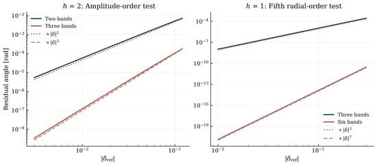
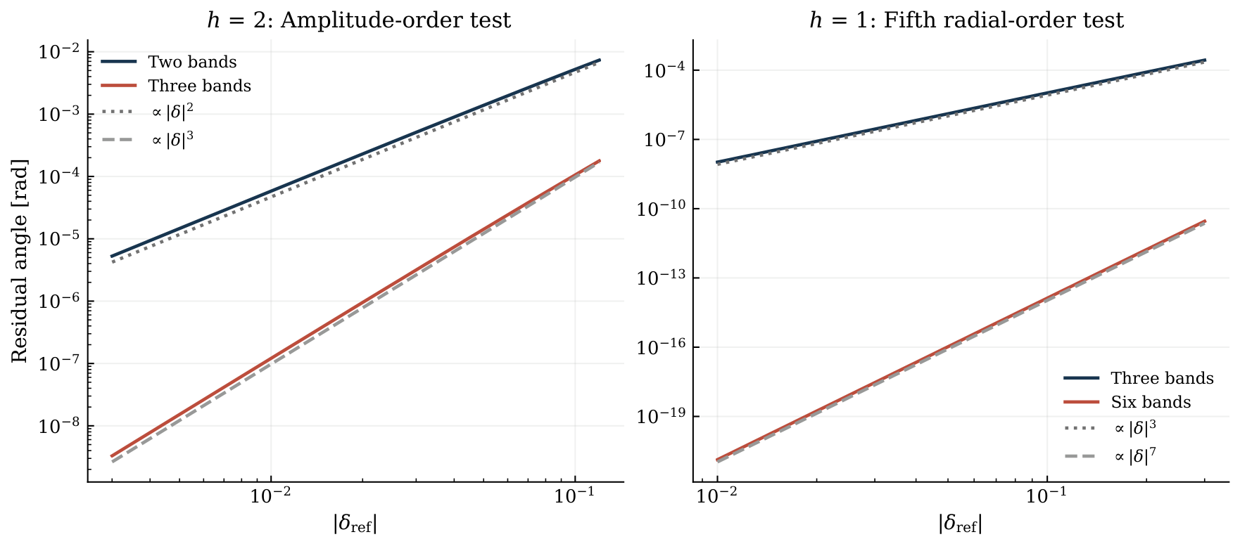
A complete fifth radial-order plasma series has a different spectral truncation. Since the susceptibility and each logarithmic derivative are proportional to x, the retained bending polynomial can contain powers through . Thus, the general fifth-order achromatic estimator uses six bands, with the same product formula for over six nodes. A seventh band tests a vanishing sixth divided difference. Three-band subtraction alone does not remove the nonlinear material terms that compete with and d. These are ordinary interpolation identities applied at the explicitly specified truncation, and do not cancel the exact dispersive angle to all orders. Figure 3 illustrates these truncation limits using exact refractive angles in flat spacetime for and . The residuals show that frequency subtraction cancels the retained spectral terms while leaving higher-order material contributions.
Figure 3.
Exact flat refractive controls for frequency subtraction. The angle exposes the quadratic two-band and cubic three-band residuals. For , gives a cubic three-band residual and a seventh-order six-band residual after the retained fifth-degree spectral terms cancel. The common nodes are successive halvings of ; all residuals are computed from exact angles.
7.4. Image Positions and the Complete Truncated Ring Equation
On the positive-image branch, asymptotic deflections enter a thin-lens forward model:
The positive aligned ring of a bending law truncated through obeys
A physical solution must be positive, connected to the relevant image branch, and within the scattering regime. The roots of the algebraic equation are not all automatically physical images.
Define , for , and . For , the root near the vacuum ring is
The small relative material shift is an additional condition, independent of weak absolute bending. Frequency combinations must compare deflections at the same B through such a forward model; image radii generally vary with frequency. Finite-distance corrections beyond this thin-lens approximation are outside the asymptotic scattering calculation.
8. Numerical Validation
8.1. Exterior Benchmark Geometries
We set in the numerical examples and retain every inverse-power term in the exact ray equation. The dimensionless coefficient vectors are
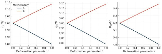
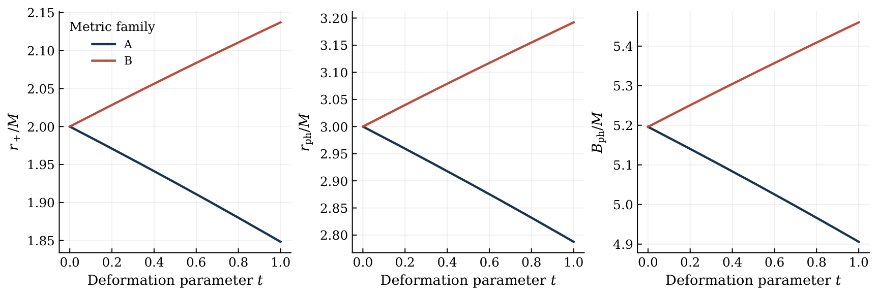
The Schwarzschild control is denoted by . Both deformed examples have an outer horizon and an exterior unstable vacuum photon orbit, with the scales in Table 1. These are choices of prescribed geometry, not fits to a source theory. The selected photon orbits satisfy . Multiplying each deformation vector by gives the continuous families in Figure 4.
Table 1.
Vacuum scales for the benchmark geometries. The largest positive horizon root and the outer unstable photon orbit are used.
Figure 4.
Outer horizon, outer unstable photon orbit, and critical vacuum impact parameter for the vectors in Equation (85), multiplied by t. Each curve uses 201 uniformly spaced points on . These vacuum scales are not dispersive capture thresholds.
8.2. Homogeneous and Inhomogeneous Comparisons
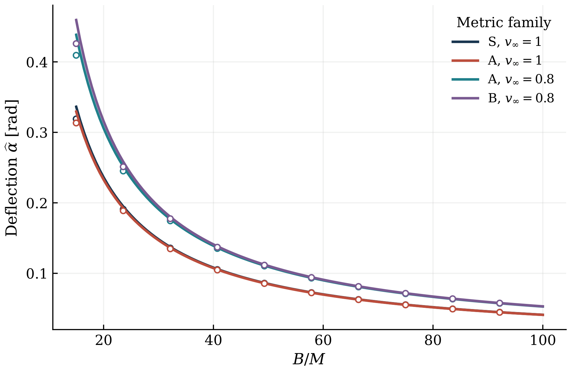
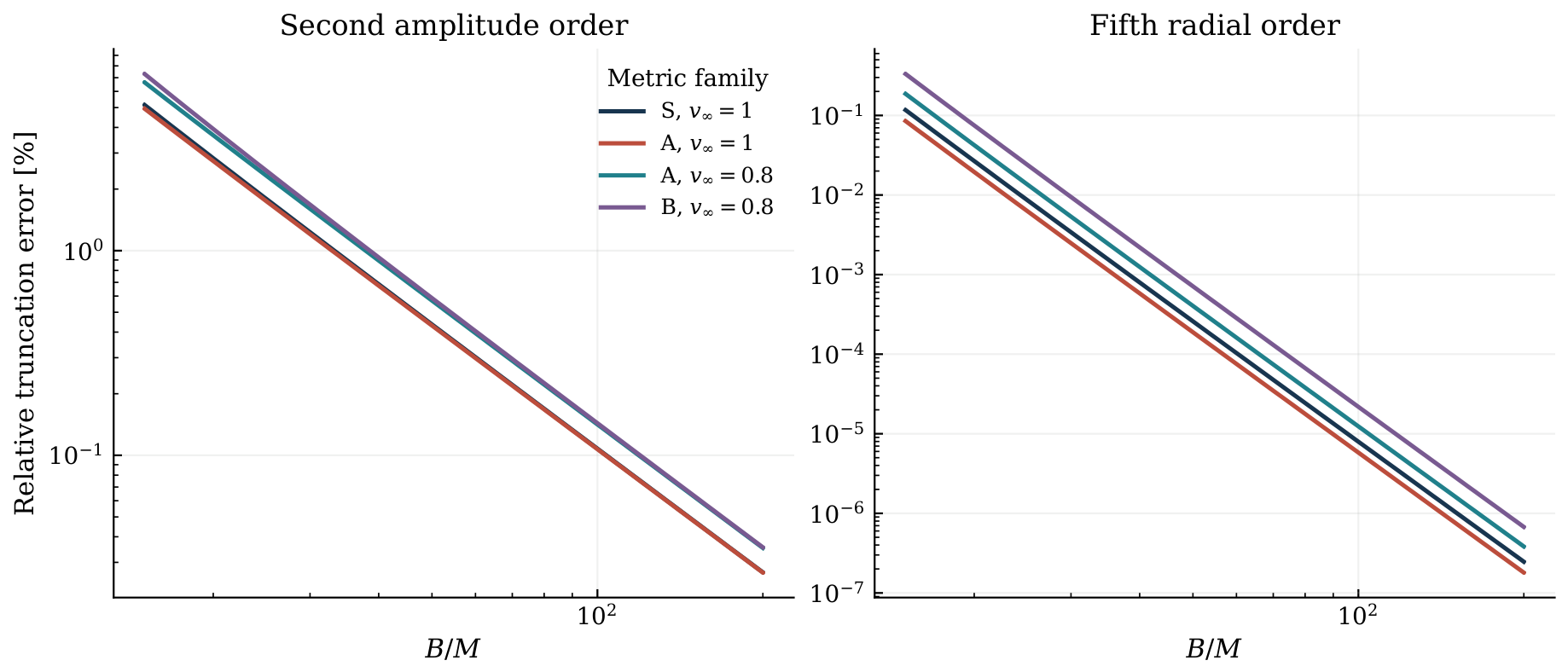
The homogeneous comparisons use the exact cold-plasma radial equation with the full lapse. Table 2 distinguishes the complete expression through the second amplitude order from the complete expression through the fifth radial order. Their error columns are . At , the displayed errors at the second amplitude order range from to , whereas retaining every radial contribution through reduces them to between and . These differences measure truncation for the specified rays. Figure 5 compares the exact homogeneous cold-plasma bending angles with the complete approximation through the second amplitude order for the selected metric families and asymptotic speeds. Figure 6 shows the corresponding relative errors and the improved accuracy obtained by retaining all contributions through the fifth radial order.
Table 2.
Exact homogeneous angles and the two distinct expansions. Angles are in radians; and are relative errors in percent. The subscript 2 denotes amplitude order, while 5 denotes radial order.
Figure 5.
Homogeneous cold-plasma angles for the indicated metric families and asymptotic speeds. Lines integrate the exact radial equation, and hollow markers show the complete expression through the second amplitude order. The common grid contains 120 uniformly spaced values .
Figure 6.
Relative errors against the same exact homogeneous rays: second amplitude order (left) and complete fifth radial order (right). Each curve uses 90 geometrically spaced values . The panels have independent vertical scales. The latter expansion includes nonlinear terms of amplitude degree higher than two.
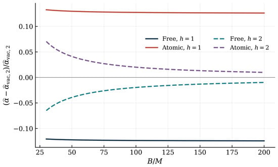
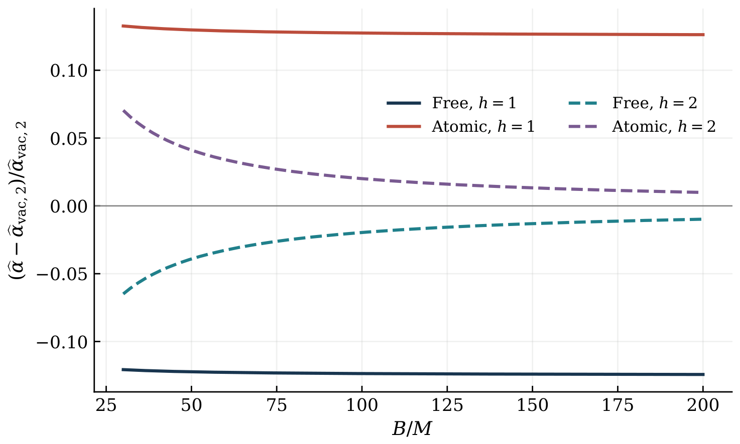
Figure 7 instead holds the medium normalization fixed while varying B. It uses family A, , and . For , the leading material fraction tends to ; for , it decays as . The plotted mixed corrections include all five contributions. The constant positive atomic susceptibility is an ideal control at frequencies far below the atomic line.
Figure 7.
Fractional material correction relative to the vacuum angle through the second amplitude order in family A. The full joint expression is used, with , , and , for free particles, or , for the ideal atomic control. There are 160 uniformly spaced points on .
8.3. Amplitude Order, Radial Order, and Independent Checks
To test the amplitude expansion without assigning higher inverse powers a higher amplitude degree, we scale every coefficient simultaneously:
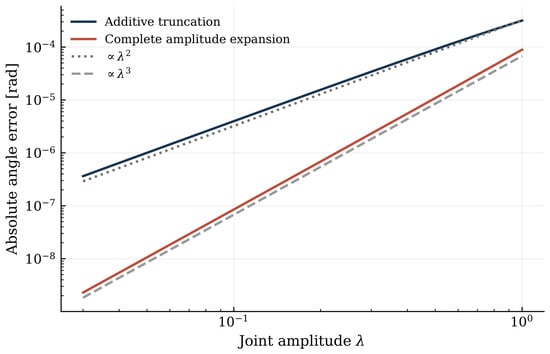
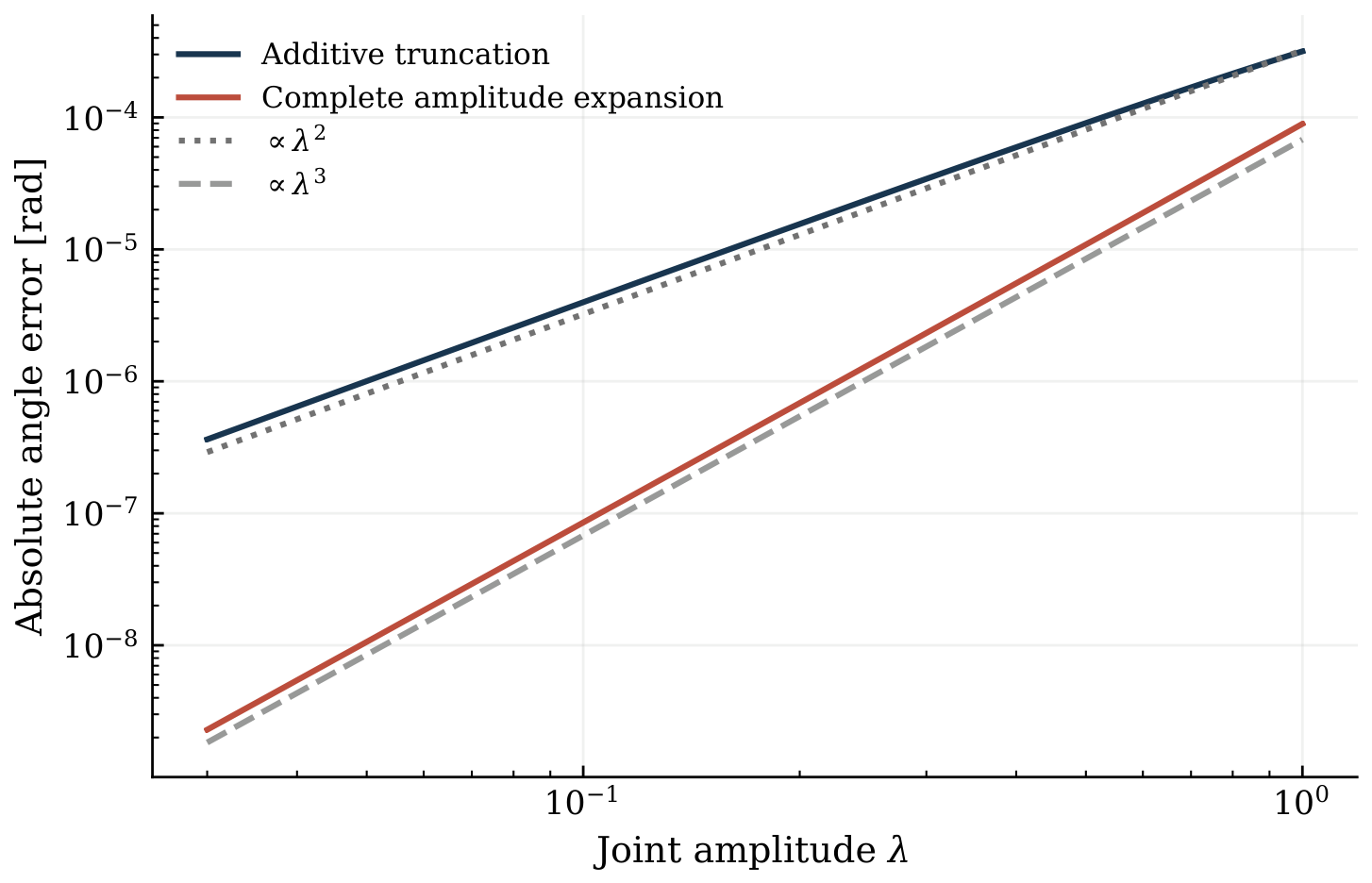
For and , the exact index is . With , the fifteen exponents range from to . Refinement to narrows the range to between and . The larger finite-scale departure occurs near cancellation of the leading cubic remainder. Figure 8 resolves the quadratic residual left by adding only leading refraction to the vacuum result through the second amplitude order.
Figure 8.
Absolute errors for Equation (86), with and . The additive comparator omits mixed and iterated material terms; the complete amplitude expression retains them. The grid has 35 geometrically spaced values . Reference lines have slopes two and three. All five metric amplitudes are scaled linearly in .
The general homogeneous formula is also tested with , where . For and the metric scaling in Equation (86), the exponents from are , , and . Independently, the complete homogeneous expansion through the fifth radial order has exponents for the absolute error ranging from to between and for the four curves of Figure 6.
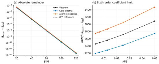
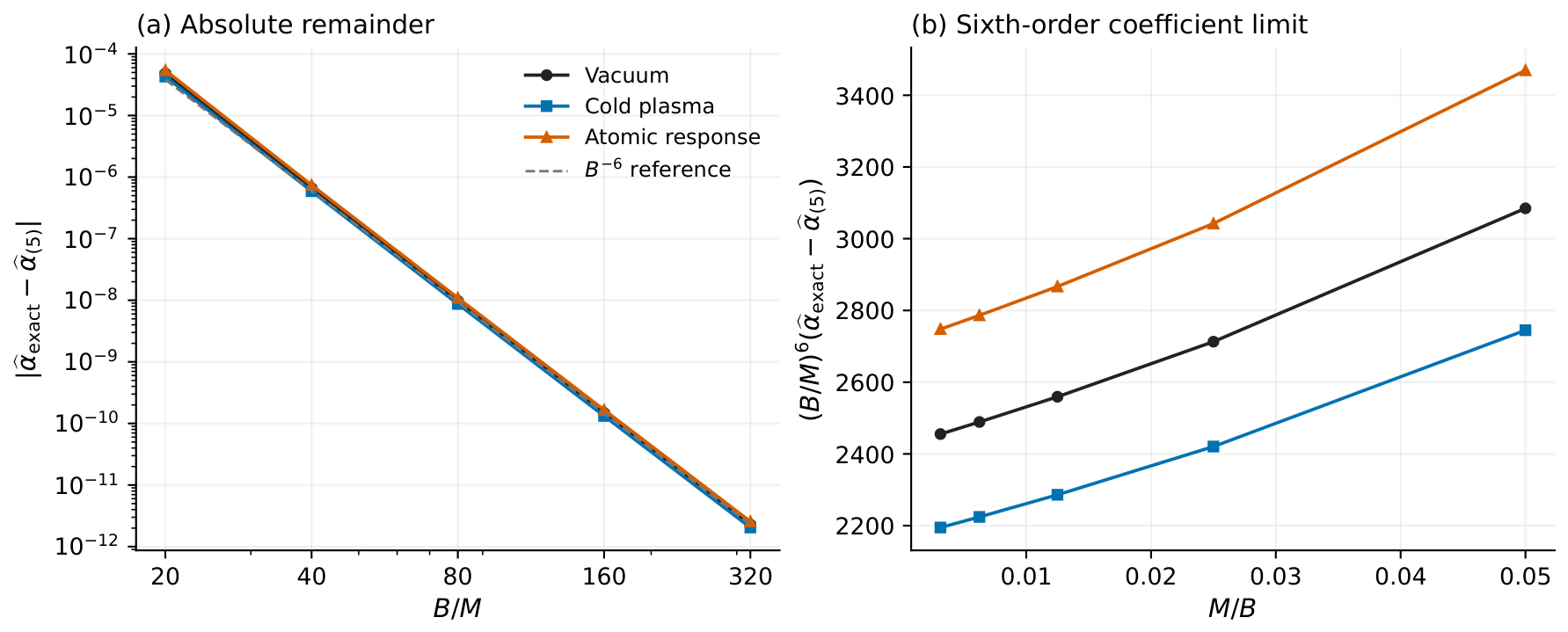
The inverse-radius medium requires a separate test through the fifth radial order because nonlinear powers of its susceptibility survive beyond the second amplitude order. Figure 9 uses an additional nonzero coefficient vector and the complete coefficients . The last exponents, from to , are in vacuum, for plasma, and for the lossless atomic response. Direct formal series inversion reproduces the coefficient generator, and the grouped formulas agree at the working precision.
Figure 9.
Complete expansion through the fifth radial order for , , , and . The controls are vacuum; at , and at , where denotes the local frequency in a fixed reference unit. Left: absolute remainder; right: the remainder multiplied by , plotted against . Exact rays include gravitational frequency shift. The five impact parameters are and 320, and the omitted leading radial order is .
We performed 74 exact algebraic checks, including the metric and material cross-terms, homogeneous reductions, radial-series identities, spectral weights, and curvature expressions. Numerical checks use independent representations of selected rays: nine Binet integrations agree with the regularized quadrature within radians, and the homogeneous Gauss–Bonnet primitive agrees within radians, for family A at , . Four evaluations of the unfactored integral at 55-digit working precision differ from double precision by at most radians. These checks apply to the specified exterior scattering rays, and do not establish a uniform error bound near capture or a response pole.
8.4. Coefficient Inference with the Complete Lapse
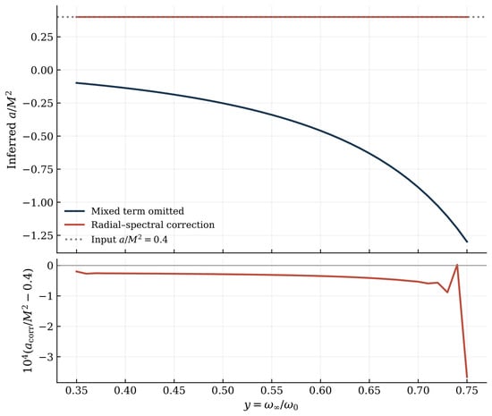
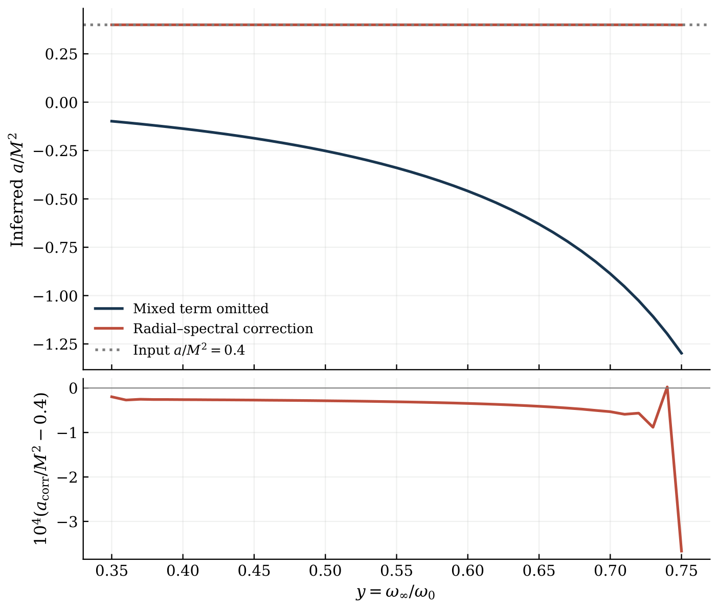
The synthetic atomic experiment tests Equation (74) in family A with , , and , where . Every exact ray retains the nonzero coefficients and evaluates the susceptibility at the local redshifted frequency. The baseline uses 41 uniformly spaced frequencies on and 45 geometrically spaced impact parameters on . Fits to in extract , with higher fit coefficients absorbing radial corrections.
Ignoring the mixed term yields to , although the input is . The invariant corrects this bias, with a baseline maximum absolute error of . Table 3 separates refinement of the frequency grid from refinement of the radial fit; 81 frequencies and a quartic fit reduce that error to . Only a is numerically reconstructed here. The presence of and d in the exact rays does not make this a simultaneous numerical recovery of all four coefficients. Figure 10 compares the naive and corrected estimates of the inverse-square metric coefficient with its input value in family A. The correction substantially reduces the material-induced bias, while the lower panel displays the remaining numerical error in this noiseless reconstruction.
Table 3.
Refinement of the family-A inference test with 45 radial points in every fit. Errors refer to ; the interior excludes the first and last two frequency nodes.
Figure 10.
Inverse-square coefficient inferred from exact lossless atomic rays in family A. The naive estimate is ; the corrected estimate replaces by . The baseline cubic radial fit and 41-frequency grid are used. The lower panel resolves the finite correction error. All higher metric coefficients remain present in the rays; no measurement noise or mass uncertainty is imposed.
The same baseline procedure in family B recovers the input with a maximum error of . All these errors describe noiseless mathematical controls. Differentiation, finite spectral coverage, and covariance would have to be included before interpreting the relation as an observational constraint.
9. Physical Domain of the Calculation
The lapse is prescribed over the exterior sampled by the rays. Its four deformation coefficients are geometrical parameters of a one-function spherical ansatz. A metric fit does not specify the underlying gravitational dynamics, and the optical calculation alone does not determine a perturbation spectrum. The numerical horizon and photon-orbit results treat the finite polynomial as exact; if it is only an asymptotic expansion, its use near those radii requires additional information about omitted terms.
A real transparent index is required along the entire path. For an atomic line with , a resonance occurs at any accessible positive root of
The generic lapse can have multiple such roots. A ray is rejected if the segment from infinity to its turning point intersects the line region, including its finite width. A frequency cutoff chosen solely at infinity is insufficient.
The intensity optical depth in the medium rest frame is
Geometrical optics also require the wavelength to be short compared with curvature and response-variation scales. At the second material order, there is a further phase-index correction. If the complex dielectric susceptibility is , with and , then
The adopted real-index law neglects this quadratic absorptive contribution, which must lie below the claimed accuracy. The complete fifth radial-order examples are strictly lossless. A finite-width application at that accuracy would require retaining the relevant complex-response corrections consistently.
An infinite absorptive profile with has divergent optical depth for , even though the idealized bending integral converges for . Similarly, an infinite homogeneous density or a mass-density power law with has divergent total mass. A physical test medium needs finite support, negligible gravitational backreaction over the relevant region, and a support or velocity model. Cold matter held at rest in a gravitational field is not a self-supported pressureless equilibrium. These idealized asymptotic profiles are useful analytic controls; finite boundaries and medium dynamics can be included only by changing the corresponding ray problem.
The cold isotropic plasma dispersion term is independent of the medium four-velocity when its scalar plasma-frequency field is prescribed. A general dispersive atomic medium does not share that simplification [48]. Warm, anisotropic, magnetized, or moving matter requires an appropriate dielectric response. The species degeneracy of cold plasma and the achromatic response degeneracies discussed above survive a formally accurate expansion.
A microscopic interpretation also requires the abundance and ionization fraction of the dark component. Constraints on atomic dark matter and collective effects depend on the particle model and cosmological or astrophysical environment [61,62]. Accordingly, the illustrative susceptibility amplitudes are not assigned a universal allowed value of . Translating a measured response into a bound on millicharge would require independent density and mass information, ordinary-plasma modeling, and a consistency check for the assumed particle population. For atoms, the binding scale and absorption spectrum supply additional model parameters.
Finally, the numerical parameter choices illustrate controlled ray scattering. They are not fitted astrophysical values. The recursive coefficient relations require radial leverage, spectral information, a mass constraint, and a material model. High-order derivatives and weak sensitivity to d at large B can make a practical inverse problem much less precise than the noiseless calculation shown here.
10. Conclusions
We have formulated dispersive weak scattering for a spherical lapse with independent inverse-radius corrections through the fifth order. Two expansions resolve the different notions of order. The complete law through the second amplitude order retains all products quadratic in the metric amplitudes and all mixed terms coupling the metric and susceptibility for a general power-law density. A separate coefficient generator gives the complete fifth-order radial law, including higher nonlinear gravitational and refractive contributions.
The radial construction yields explicit vacuum coefficients and a complete hierarchy for a medium with an inverse-radius susceptibility. This hierarchy depends on the response and its first four logarithmic frequency derivatives. The third coefficient already contains a cubic refractive term that survives in flat spacetime. Keeping these terms is essential when material effects are compared with the cubic and quintic metric corrections. Independent checks using exact rays and formal series reproduce the predicted amplitude and radial remainders.
Within the assigned inverse-radius index model and with the mass constrained, the coefficient map is triangular. The leading radial coefficient and its spectral derivatives determine the material terms needed to reconstruct the four metric coefficients successively. The experiment using exact rays illustrates the inverse-square coefficient in the presence of all higher metric terms, while the practical recovery of the higher coefficients remains sensitive to derivative noise and radial conditioning. Additional material profiles create calculable degeneracies.
Frequency subtraction must follow the same ordering as the bending law. Three bands cancel the quadratic plasma spectral model of the amplitude expansion, whereas the general fifth-order radial plasma polynomial requires six bands. The corresponding null relations test the retained spectral form at a common impact parameter. Image positions require a forward lens model, for which the complete truncated aligned-ring equation has been given.
The millicharged examples connect this framework to two distinct microscopic responses. Free dark charges contribute according to their squared charge multiplied by the number density and divided by particle mass, and share the dispersion of ordinary cold plasma. Their contribution can therefore be included consistently in geometric inference, although the bending law alone determines only the summed plasma response. Neutral dark atoms introduce a binding scale and dynamical polarizability. Their response is nearly achromatic far below the first electric-dipole transition, and becomes more dispersive as that scale is approached within a transparent window. The resulting spectral derivatives enter the mixed gravitational and material terms explicitly. Together, these examples explain how the abundance, ionization state, and internal structure of an interacting dark component can bias a vacuum interpretation, and what additional material information is needed to separate it from the exterior geometry.
The generic geometry and transparent test-medium assumptions define the scope of these results. Applications to a particular compact object require a justified exterior metric, a finite supported medium, and control of absorption and frequency matching. The derived formulas provide explicit checks on how material response enters geometric inference at successive radial orders.
Funding
This research received no external funding.
Data Availability Statement
No external observational data were used. The equations, numerical parameters, fitting procedure, and validation results are presented in the article.
Acknowledgments
ChatGPT-6 Astra (OpenAI) assisted with figure preparation and language revision.
Conflicts of Interest
The author declares no conflicts of interest.
Appendix A. Derivation of the Kernels Through the Second Amplitude Order
This derivation uses the normalized optical impact radius in Equation (36). Define
Thus, the exact kernel in the main text is . We write its deviation from the asymptotic value as . The expansion is performed on the outer branch where is monotone; the turning point remains at its exact optical value .
For the decaying susceptibility, . Put
with S and evaluated at . Since and the susceptibility and its derivatives are first-order amplitudes,
In particular, the term due to frequency redshift has the same retained amplitude degree as the products of metric and susceptibility perturbations.
Expanding at a fixed areal radius gives
These expressions alone do not give the coefficient of the angle, because the integration variable is p, rather than r. Inverting yields
The last term incorporates the displacement of the trajectory and the coordinate turning point.
Let , and evaluate at p in the following expression. Using , , and , the complete kernel is
The double sum is ordered. For a monomial with , Equation (37) gives
Applying this identity to Equation (A6), with , proves Equation (41). It also shows why the mixed terms involving and d are of the same amplitude degree as the term coupling mass and response, even though their radial powers differ.
For a homogeneous response, write and expand . With , the optical logarithm becomes
The same composition rule then gives
Equation (A7) proves the general homogeneous result, Equation (47). Setting recovers the vacuum kernel; the homogeneous cold-plasma derivatives give the velocity-dependent expression in the main text. This derivation expands in metric amplitudes while keeping the homogeneous susceptibility dependence through its actual spectral derivatives.
Appendix B. Numerical Integration and Fitting Procedure
The numerical calculations evaluate the displayed lapse directly, with B distinct from the metric coefficient b. For numerical controls, we set and express and d in the corresponding powers of M. The root selection and numerical tolerances below apply to the tested weak-scattering domain.
The first accessible simple zero of in Equation (35) is bracketed before any detected horizon or atomic pole. Polynomial roots determine candidate horizons and line crossings. The turning point is located by scanning for a sign change and refining the bracket with the Brent method using an absolute tolerance of and a relative tolerance of . The accepted interval is sampled to check and . These numerical checks are sufficient for the smooth weak rays used here; they are not a proof of global root isolation for arbitrary coefficients.
We remove the square-root endpoint by setting :
Near the root, we evaluate using factored polynomial differences and numerically stable evaluations of logarithmic and exponential differences for noninteger powers. This avoids subtracting nearly equal terms. Adaptive quadrature uses absolute and relative tolerances of ; these requested tolerances are not certified error bounds. Independent integrations of the unfactored integrand use 55-digit working precision. The Binet check integrates from to the returning , using DOP853, a relative tolerance of , an absolute tolerance of , and a maximum angular step of .
For the joint expansion, the exact power-response model is
The fifteen control families use and . The primary sequence is , with refinement to . This scales every metric and response amplitude together. Taking at fixed dimensional coefficients instead tests the radial expansion. The full fifth-order homogeneous and inverse-radius-medium tests use and higher-precision radial integration to resolve the small remainder.
The atomic coefficient experiment uses the lossless response
The exact index is . At each frequency, 45 logarithmically spaced impact parameters in give the fitting data. We fit as a polynomial in , normalize the design-matrix columns, and solve by singular-value least squares. In units , the intercept is , and is 100 times the linear coefficient. Cubic and quartic fits use the same rays. The unscaled design-matrix condition numbers are and , respectively. A not-a-knot cubic spline of against supplies the derivative in Equation (74). The interior error excludes the two outermost frequency nodes on each side. All reported errors are deterministic deviations from the specified input, without observational noise or a fitted covariance model.
The spectral-subtraction controls use exact flat-medium laws,
The six-band calculation uses 60-digit arithmetic to avoid cancellation at small susceptibility. For nodes , its weights are
The norm is the standard-deviation amplification for independent equal-error bands. The three-band nodes have weights and a norm of . Correlated errors require instead of the equal-noise expression.
The stated equations, sampling grids, integration tolerances, and fitting prescriptions specify the numerical procedures used for the figures and tables. Working precision and numerical agreement are reported separately; no calculation here certifies a global error bound outside the tested domain.
References
- Virbhadra, K.S.; Ellis, G.F.R. Gravitational lensing by naked singularities. Phys. Rev. D 2002, 65, 103004. [Google Scholar] [CrossRef] [Scilit]
- Virbhadra, K.S.; Keeton, C.R. Time delay and magnification centroid due to gravitational lensing by black holes and naked singularities. Phys. Rev. D 2008, 77, 124014. [Google Scholar] [CrossRef] [Scilit]
- Virbhadra, K.S. Relativistic images of Schwarzschild black hole lensing. Phys. Rev. D 2009, 79, 083004. [Google Scholar] [CrossRef] [Scilit]
- Virbhadra, K.S. Distortions of images of Schwarzschild lensing. Phys. Rev. D 2022, 106, 064038. [Google Scholar] [CrossRef] [Scilit]
- Virbhadra, K.S. Conservation of distortion of gravitationally lensed images. Phys. Rev. D 2024, 109, 124004. [Google Scholar] [CrossRef] [Scilit]
- do Carmo, M.P. Riemannian Geometry; Birkhäuser: Boston, MA, USA, 1992. [Google Scholar] [CrossRef] [Scilit]
- Nakahara, M. Geometry, Topology and Physics, 2nd ed.; Institute of Physics Publishing: Bristol, UK, 2003. [Google Scholar]
- Gibbons, G.W.; Werner, M.C. Applications of the Gauss-Bonnet theorem to gravitational lensing. Class. Quantum Grav. 2008, 25, 235009. [Google Scholar] [CrossRef] [Scilit]
- Werner, M.C. Gravitational lensing in the Kerr-Randers optical geometry. Gen. Relativ. Gravit. 2012, 44, 3047–3057. [Google Scholar] [CrossRef] [Scilit]
- Ishihara, A.; Suzuki, Y.; Ono, T.; Kitamura, T.; Asada, H. Gravitational bending angle of light for finite distance and the Gauss-Bonnet theorem. Phys. Rev. D 2016, 94, 084015. [Google Scholar] [CrossRef] [Scilit]
- Ishihara, A.; Suzuki, Y.; Ono, T.; Asada, H. Finite-distance corrections to the gravitational bending angle of light in the strong deflection limit. Phys. Rev. D 2017, 95, 044017. [Google Scholar] [CrossRef] [Scilit]
- Ono, T.; Ishihara, A.; Asada, H. Gravitomagnetic bending angle of light with finite-distance corrections in stationary axisymmetric spacetimes. Phys. Rev. D 2017, 96, 104037. [Google Scholar] [CrossRef] [Scilit]
- Rindler, W.; Ishak, M. Contribution of the cosmological constant to the relativistic bending of light revisited. Phys. Rev. D 2007, 76, 043006. [Google Scholar] [CrossRef] [Scilit]
- Gibbons, G.W.; Warnick, C.M.; Werner, M.C. Light-bending in Schwarzschild-de Sitter: Projective geometry of the optical metric. Class. Quantum Grav. 2008, 25, 245009. [Google Scholar] [CrossRef] [Scilit]
- Arakida, H. Light deflection and Gauss-Bonnet theorem: Definition of total deflection angle and its applications. Gen. Relativ. Gravit. 2018, 50, 48. [Google Scholar] [CrossRef] [Scilit]
- Takizawa, K.; Ono, T.; Asada, H. Gravitational deflection angle of light: Definition by an observer and its application to an asymptotically nonflat spacetime. Phys. Rev. D 2020, 101, 104032. [Google Scholar] [CrossRef] [Scilit]
- Adler, S.L.; Virbhadra, K.S. Cosmological constant corrections to the photon sphere and black hole shadow radii. Gen. Relativ. Gravit. 2022, 54, 93. [Google Scholar] [CrossRef] [Scilit]
- Li, Z.; Zhou, T. Equivalence of Gibbons-Werner method to geodesics method in the study of gravitational lensing. Phys. Rev. D 2020, 101, 044043. [Google Scholar] [CrossRef] [Scilit]
- Li, Z.; Zhang, G.; Övgün, A. Circular orbit of a particle and weak gravitational lensing. Phys. Rev. D 2020, 101, 124058. [Google Scholar] [CrossRef] [Scilit]
- Övgün, A.; Pantig, R.C. Boundary-only weak deflection angles from isothermal optical geometry. Class. Quantum Grav. 2026, 43, 085011. [Google Scholar] [CrossRef] [Scilit]
- Övgün, A.; Pantig, R.C. Radial integral reformulation of the Gauss-Bonnet weak deflection angle at finite distance. Chin. J. Phys. 2026, 103, 1523–1535. [Google Scholar] [CrossRef] [Scilit]
- Pantig, R.C.; Övgün, A. Reference-renormalized curvature-primitive Gauss-Bonnet formalism for finite-distance weak gravitational lensing in static spherical spacetimes. Phys. Rev. D 2026, 113, 104037. [Google Scholar] [CrossRef] [Scilit]
- Pantig, R.C.; Övgün, A. Gauss-Bonnet lensing of spinning massive particles in static spherically symmetric spacetimes. Ann. Phys. 2026, 488, 170421. [Google Scholar] [CrossRef] [Scilit]
- Claudel, C.-M.; Virbhadra, K.S.; Ellis, G.F.R. The geometry of photon surfaces. J. Math. Phys. 2001, 42, 818–838. [Google Scholar] [CrossRef] [Scilit]
- Bozza, V. Gravitational lensing in the strong field limit. Phys. Rev. D 2002, 66, 103001. [Google Scholar] [CrossRef] [Scilit]
- Tsukamoto, N. Deflection angle in the strong deflection limit in a general asymptotically flat, static, spherically symmetric spacetime. Phys. Rev. D 2017, 95, 064035. [Google Scholar] [CrossRef] [Scilit]
- Tsukamoto, N. Deflection angle of a light ray reflected by a general marginally unstable photon sphere in a strong deflection limit. Phys. Rev. D 2020, 102, 104029. [Google Scholar] [CrossRef] [Scilit]
- Sasaki, T. Strong gravitational lensing by a Reissner-Nordström naked singularity with a marginally unstable photon sphere. Phys. Rev. D 2025, 112, 024072. [Google Scholar] [CrossRef] [Scilit]
- Igata, T.; Sasaki, T.; Tsukamoto, N. Strong-deflection expansion of the deflection angle near a degenerate photon sphere. Phys. Rev. D 2026, 113, 104022. [Google Scholar] [CrossRef] [Scilit]
- Tsukamoto, N. Gravitational lensing inside and outside of a marginally unstable photon sphere in a general, static, spherically symmetric, and asymptotically flat spacetime in strong deflection limits. Phys. Rev. D 2026, 113, 104016. [Google Scholar] [CrossRef] [Scilit]
- Igata, T. Deflection angle in the strong deflection limit: A perspective from local geometrical invariants and matter distributions. Phys. Rev. D 2026, 113, 044042. [Google Scholar] [CrossRef] [Scilit]
- Cardoso, V.; Miranda, A.S.; Berti, E.; Witek, H.; Zanchin, V.T. Geodesic stability, Lyapunov exponents and quasinormal modes. Phys. Rev. D 2009, 79, 064016. [Google Scholar] [CrossRef] [Scilit]
- Stefanov, I.Z.; Yazadjiev, S.S.; Gyulchev, G.G. Connection between black-hole quasinormal modes and lensing in the strong deflection limit. Phys. Rev. Lett. 2010, 104, 251103. [Google Scholar] [CrossRef] [Scilit] [PubMed]
- Pantig, R.C.; Mastrototaro, L.; Lambiase, G.; Övgün, A. Shadow, lensing, quasinormal modes, greybody bounds and neutrino propagation by dyonic ModMax black holes. Eur. Phys. J. C 2022, 82, 1155. [Google Scholar] [CrossRef] [Scilit]
- Lütfüoğlu, B.C.; Rayimbaev, J.; Murodov, S.; Kurbanov, J.; Matyoqubov, M. A first-order eikonal framework for quasinormal modes, shadows, strong lensing, and grey-body factors in a scalarized black-hole metric. Ann. Phys. 2026, 491, 170514. [Google Scholar] [CrossRef] [Scilit]
- Pantig, R.C.; Övgün, A. Gravitational black hole shadow spectroscopy. Phys. Rev. D 2025, 112, 124072. [Google Scholar] [CrossRef] [Scilit]
- Övgün, A.; Pantig, R.C.; Saavedra, J. Redshift spectroscopy as a probe of regular black holes, black bounces, and scalar-hair compact objects. Phys. Dark Universe 2026, 53, 102392. [Google Scholar] [CrossRef] [Scilit]
- Synge, J.L. Relativity: The General Theory; North-Holland: Amsterdam, The Netherlands, 1960. [Google Scholar]
- Perlick, V. Ray Optics, Fermat’s Principle, and Applications to General Relativity; Lecture Notes in Physics Monographs; Springer: Berlin/Heidelberg, Germany, 2000; Volume 61. [Google Scholar]
- Bisnovatyi-Kogan, G.S.; Tsupko, O.Y. Gravitational lensing in a non-uniform plasma. Mon. Not. R. Astron. Soc. 2010, 404, 1790–1800. [Google Scholar] [CrossRef] [Scilit]
- Crisnejo, G.; Gallo, E. Weak lensing in a plasma medium and gravitational deflection of massive particles using the Gauss-Bonnet theorem: A unified treatment. Phys. Rev. D 2018, 97, 124016. [Google Scholar] [CrossRef] [Scilit]
- Crisnejo, G.; Gallo, E.; Villanueva, J.R. Gravitational lensing in dispersive media and deflection angle of charged massive particles in terms of curvature scalars and energy-momentum tensor. Phys. Rev. D 2019, 100, 044006. [Google Scholar] [CrossRef] [Scilit]
- Crisnejo, G.; Gallo, E.; Jusufi, K. Higher order corrections to deflection angle of massive particles and light rays in plasma media for stationary spacetimes using the Gauss-Bonnet theorem. Phys. Rev. D 2019, 100, 104045. [Google Scholar] [CrossRef] [Scilit]
- Comberiati, F.; de la Cruz, L. Gravitational lensing in a plasma from worldlines. Phys. Rev. D 2025, 111, 054030. [Google Scholar] [CrossRef] [Scilit]
- Tsupko, O.Y. Deflection of light rays by a spherically symmetric black hole in a dispersive medium. Phys. Rev. D 2021, 103, 104019. [Google Scholar] [CrossRef] [Scilit]
- Perlick, V.; Tsupko, O.Y.; Bisnovatyi-Kogan, G.S. Influence of a plasma on the shadow of a spherically symmetric black hole. Phys. Rev. D 2015, 92, 104031. [Google Scholar] [CrossRef] [Scilit]
- Perlick, V.; Tsupko, O.Y. Light propagation in a plasma on Kerr spacetime: Separation of the Hamilton-Jacobi equation and calculation of the shadow. Phys. Rev. D 2017, 95, 104003. [Google Scholar] [CrossRef] [Scilit]
- Bezděková, B.; Tsupko, O.Y.; Pfeifer, C. Deflection of light rays in a moving medium around a spherically symmetric gravitating object. Phys. Rev. D 2024, 109, 124024. [Google Scholar] [CrossRef] [Scilit]
- Övgün, A.; Pantig, R.C.; Lambiase, G. Dispersive and absorbing effects of dusty plasma on black hole lensing, shadows, and eikonal ringdown. Phys. Dark Universe 2026, 52, 102341. [Google Scholar] [CrossRef] [Scilit]
- Atamurotov, F.; Ortiqboev, D.; Abdujabbarov, A.; Mustafa, G. Particle dynamics and gravitational weak lensing around black hole in the Kalb-Ramond gravity. Eur. Phys. J. C 2022, 82, 659. [Google Scholar] [CrossRef] [Scilit]
- Pahlavon, Y.; Atamurotov, F.; Bouzenada, A.; Abdujabbarov, A.; Mustafa, G. Deflection angle around generic traversable wormhole solutions and energy conditions in extended teleparallel theory of gravity. Nucl. Phys. B 2025, 1014, 116882. [Google Scholar] [CrossRef] [Scilit]
- Ali, R.; Xia, T.; Awais, M.; Babar, R. Deflection angle and shadow evolution from charged torus-like black hole under the effect of non-magnetic plasma and non-plasma medium. Int. J. Geom. Methods Mod. Phys. 2024, 21, 2450180. [Google Scholar] [CrossRef] [Scilit]
- Holdom, B. Two U(1)’s and epsilon charge shifts. Phys. Lett. B 1986, 166, 196–198. [Google Scholar] [CrossRef] [Scilit]
- Gardner, S.; Latimer, D.C. Dark matter constraints from a cosmic index of refraction. Phys. Rev. D 2010, 82, 063506. [Google Scholar] [CrossRef] [Scilit]
- Latimer, D.C. Dispersive light propagation at cosmological distances: Matter effects. Phys. Rev. D 2013, 88, 063517. [Google Scholar] [CrossRef] [Scilit]
- Övgün, A. Deflection angle of photons through dark matter by black holes and wormholes using the Gauss-Bonnet theorem. Universe 2019, 5, 115. [Google Scholar] [CrossRef] [Scilit]
- Kaplan, D.E.; Krnjaic, G.Z.; Rehermann, K.R.; Wells, C.M. Atomic dark matter. J. Cosmol. Astropart. Phys. 2010, 05, 021. [Google Scholar] [CrossRef] [Scilit]
- Kaplan, D.E.; Krnjaic, G.Z.; Rehermann, K.R.; Wells, C.M. Dark atoms: Asymmetry and direct detection. J. Cosmol. Astropart. Phys. 2011, 10, 011. [Google Scholar] [CrossRef] [Scilit]
- Kvam, A.K.; Latimer, D.C. Astrophysical constraints on millicharged atomic dark matter. arXiv 2014, arXiv:1412.0708. [Google Scholar]
- Kvam, A.K.; Latimer, D.C. Optical dispersion of composite particles consisting of millicharged constituents. J. Phys. G Nucl. Part. Phys. 2016, 43, 085002. [Google Scholar] [CrossRef] [Scilit]
- Bansal, S.; Barron, J.; Curtin, D.; Tsai, Y. Precision cosmological constraints on atomic dark matter. J. High Energy Phys. 2023, 10, 095. [Google Scholar] [CrossRef] [Scilit]
- Cruz, A.; McQuinn, M. Astrophysical plasma instabilities induced by long-range interacting dark matter. J. Cosmol. Astropart. Phys. 2023, 2023, 028. [Google Scholar] [CrossRef] [Scilit]
- Aalbers, J.; Akerib, D.S.; Musalhi, A.K.A.; Alder, F.; Amarasinghe, C.S.; Ames, A.; Anderson, T.J.; Angelides, N.; Araújo, H.M.; Armstrong, J.E.; et al. First constraint on atmospheric millicharged particles with the LUX-ZEPLIN experiment. Phys. Rev. Lett. 2025, 134, 241802. [Google Scholar] [CrossRef] [Scilit] [PubMed]
- Jia, J. The perturbative approach for the weak deflection angle. Eur. Phys. J. C 2020, 80, 242. [Google Scholar] [CrossRef] [Scilit]
- Li, G.; Li, Z.; Jia, J. Light deflection in general static and spherically symmetric spacetime with a homogeneous plasma. arXiv 2026, arXiv:2607.22401. [Google Scholar] [CrossRef] [Scilit]

Disclaimer/Publisher’s Note: The statements, opinions and data contained in all publications are solely those of the individual author(s) and contributor(s) and not of MDPI and/or the editor(s). MDPI and/or the editor(s) disclaim responsibility for any injury to people or property resulting from any ideas, methods, instructions or products referred to in the content. |
© 2026 by the author. Licensee MDPI, Basel, Switzerland. This article is an open access article distributed under the terms and conditions of the Creative Commons Attribution (CC BY) license.