Finite-Time Output Feedback Control for Electro-Hydraulic Servo Systems with Parameter Adaptation

Abstract

Measurement noise, parametric uncertainties, and external disturbances broadly exist in electro-hydraulic servo systems, which terribly deteriorate the system control performance. To figure out this problem, a novel finite-time output feedback controller with parameter adaptation is proposed for electro-hydraulic servo systems in this paper. First, to avoid using noise-polluted signals and attain active disturbance compensation, a finite-time state observer is adopted to estimate unknown system states and disturbances, which attenuates the impact of measurement noise and external disturbances on tracking performance. Second, by adopting a parameter adaptive law, the parametric uncertainties in the electro-hydraulic servo system can be much lessened, which is beneficial to averting the high-gain feedback in practice. Then, integrating the backstepping framework and the super-twisting sliding mode technique, a synthesized output feedback controller is constructed to achieve high-accuracy tracking performance for electro-hydraulic servo systems. Lyapunov stability analysis demonstrates that the proposed control scheme can acquire finite-time stability. The excellent tracking performance of the designed control law is verified by comparative simulation results.

1. Introduction

Hydraulic servo systems have been widely used in modern industry [1,2,3,4,5] due to their good capabilities such as high power/weight ratio, large output force, etc. However, the electro-hydraulic servo system is a sort of highly non-linear system with various model uncertainties which is mainly manifested in the non-linear pressure and flow of the valve. The model uncertainties of the electro-hydraulic servo system can be divided into parameter uncertainties and uncertain nonlinearities, such as parameter change, external disturbances, nonlinear friction and so on. These problems have always restricted the development of advanced control and the decision-making algorithms for electro-hydraulic servo systems. The modeling uncertainties will seriously deteriorate the performance of the designed controller and lead to cycle oscillations and even instability in the system [6]. With the development of the industry, there is increasingly high demanding for the control speed and accuracy of the hydraulic system. Thus, the traditional linear control methods have become more and more difficult to satisfy the demand of modern hydraulic servo systems. In order to solve the above problems, non-linear system controllers have been expanded in the past few decades, such as robust control [7], H infinity control [8,9,10], and adaptive control [11,12,13]. Among these methods, adaptive control can cope with parametric variations due to its learning ability.

The adaptive control (AC) [3] was generally used to deal with parameter uncertainties, but it had little effect on unmodeled disturbances. The adaptive robust control (ARC) in [14,15] could simultaneously solve the unmodeled disturbances and parameter uncertainties. However, ARC could only guarantee the bounded tracking performance when dealing with unmodeled disturbances. In order to solve the unknown nonlinearities that cannot be presented in the form of linear parameterization, function approximators have been researched, such as neural networks (NN) [16,17,18,19] and fuzzy systems (FS) [20,21,22]. However, these function approximators might bring heavy computational costs and require a considerable amount of time to achieve convergence, which was also affected by the adopted adaptive law and learning gains.

Sliding mode control can often be employed to handle bounded modeling uncertainties and to obtain asymptotic tracking performance in hydraulic systems [23]. However, the discontinuity of the control input will cause the controller chattering, which is not allowed for the actual hydraulic systems. In order to eliminate chattering in the sliding mode control, a continuous saturation function instead of a discontinuous sign function was used in [24], but it could only ensure bounded tracking performance [25]. The high-order sliding mode controller designed in [26] could obtain asymptotic tracking while ensuring the continuity of the controller. However, the designing process of the controller required the derivative of the sliding mode, which was difficult to implement in engineering. Super-twisting sliding mode control in [27,28] could not only retain the high robustness, but also solve the high frequency chattering problem. Additionally, as the second-order sliding mode algorithm, the super-twisting sliding mode control could also obtain finite-time stability. In 2006, a review article in a book by Dorato explained the strong robustness of finite-time stability [29], which pointed out the difference between finite-time stability and the stability under traditional concepts. In the meanwhile, the superiority of this method in transient response performance was proved. Based on this method, many results have been achieved [30,31,32,33,34,35]. Unfortunately, none of the above controllers have considered the uncertainties of the system parameters. In [36], some researchers proposed the finite time control with parameter adaptation. However, most of them were for linear systems. An adaptive finite-time controller for nonlinear systems with parametric uncertainties was proposed in [37]. This controller based on backstepping methodology could not only realize the finite-time stability in the nonlinear system, but also synthesize the advantages of parameter adaptation. Nevertheless, the condition that all system states in the above-mentioned literature need to be known, is not easy to be satisfied in practice.

Backstepping methodology is used in most of the existing electro-hydraulic system control [38]. In these backstepping designs, the entire system state must be known or measurable due to the strict backstepping process. However, the velocity and acceleration signals in hydraulic systems are usually unmeasurable due to lack of sensors. Though they can be acquired by numerical differentiation on the position measurement, the obtained velocity and acceleration signals are accompanied by strong measurement noise. Therefore, in order to avoid using these variables in the control design, some output feedback controllers that only uses measurable output for practical application have been developed. In [39], an output feedback controller based on extend state observer was proposed to estimate the unmeasurable state variables through output variables, but it could only guarantee global uniformly ultimately bounded tracking performance. In [40], an output feedback control based on a finite-time observer was proposed, but it did not consider parameter adaptation. In [41], Levant proposed an output-feedback controller based on a higher-order sliding mode differentiation. Compared with the extended state observer, the finite-time observer has better transient response performance.

Motivated by the above observations, the following problems are expected to be resolved in this paper: (1) avoid using the noise-contaminated velocity and acceleration signals in the control design; (2) eliminate the high-gain feedback issue in the existing sliding mode control methods; and (3) achieve the excellent finite-time tracking performance with zero steady-state error for the electro-hydraulic servo system. Therefore, a finite-time output feedback controller with parameter adaptation (FOFA) is proposed for electro-hydraulic servo systems in this paper. In order to complete this research, a nonlinear model of the electro-hydraulic servo system considering the parameter uncertainties and external disturbances is established. Aiming at the stability problem of the electro-hydraulic servo system under the condition of parameter uncertainties and system disturbances, this paper adopts a parameter adaptive law to remove the parametric uncertainties. Then integrating the backstepping framework and the super-twisting sliding mode technique, a composite output feedback controller is designed to achieve high-accuracy tracking performance for electro-hydraulic servo systems. Parameter adaptation and super-twisting sliding mode are combined in an innovative way, and feedforward compensation is performed through parameter adaptation, which can effectively prevent system instability caused by high-gain feedback and achieve finite time stability. Also, an output feedback control method realized by finite-time observer is combined to achieve the estimations of unknown system states and to compensate for the unmodeled and external disturbances. Lyapunov stability analysis demonstrates that the proposed control scheme can acquire finite-time stability, and the excellent tracking performance of the designed control law is verified by comparative simulation results.

The organization structure of this paper is as follows: Section 2 presents the problem formation and dynamic model. Section 3 presents the design process and theoretical results of finite time observer and adaptive law of the finite time output feedback controller proposed in this paper. Section 4 provides the simulation settings and comparison of results. Section 5 discusses the conclusion.

2. Dynamic Model and Problem Formulation

The equipment considered in this paper is descripted in Figure 1. Our purpose is to ensure that the tracking output can track the desired trajectory as closely as possible. The dynamic equation of the inertial load of the servo system can be described as follows:

$$m\ddot{y}=A(P_1-P_2)-B\dot{y}+L(t)$$

(1)

where y represents the displacement and m represents the inertial mass of load; $P_L=P_1-P_2$ stands for the load pressure of hydraulic actuator, in which $P_1$ and $P_2$ are the pressures inside two chambers of the hydraulic cylinders, separately; $A$ denotes the effective area of ram of the two chambers, B represents viscous friction coefficient, and L(t) represents the external and unmodeled disturbances of the hydraulic cylinders.

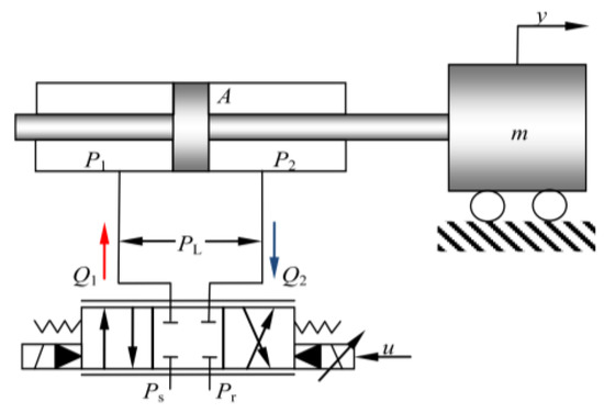
Figure 1. Schematic diagram of the hydraulic actuator system.

The load pressure dynamics can be written as

$$\frac{V_t}{4{\beta }_e}{\dot{P}}_L=-A\dot{y}-C_t{P}_L+Q_E+Q_L$$

(2)

where $V_t$ is the total control volume of the actuator; ${\beta }_e$ is the effective oil bulk modulus; $C_t$ represents the internal leakage coefficient of the chambers due to pressure; $Q_E$ is the time-varying modeling error caused by complicated internal leakage, parameter deviations, unmodeled pressure dynamics, modeling error caused by the following flow equation, and so on; $Q_L=\left(Q_1+Q_2\right)/2$ is the load flow; $Q_1$ is the supplied flow rate to the forward chamber; and $Q_2$ is the return flow rate of the return chamber. According to [4], $Q_L$ is related to the spool valve displacement of the servo valve, and it can be deduced that

$$Q_L=k_q{x}_v\sqrt{P_s-sign\left(x_v\right)P_L}$$

(3)

where $k_q=C_{d}w\sqrt{1/\tau }$ represents the flow rate gain, $C_d$ is the discharge coefficient; $x_v$ is the spool valve displacement of the servo valve; $P_s$ is the supply pressure of the fluid with respect to the return pressure $P_r$; and sign (·) denotes the standard signum function as

$$sign\left(x_v\right)=\{\begin{array}{c}1 \mathrm{if} x_v>0\\ 0 \mathrm{if} x_v=0\\ -1 \mathrm{if} x_v<0\end{array}$$

(4)

The effects of servo-valve dynamics have been included by some researchers [42,43]. However, additional sensors are required to obtain the spool position, and only minimal performance improvement can be achieved for motion tracking. In addition, valve dynamics will increase the system order and complicate the controller design. Therefore, many literatures neglect servo-valve dynamics. Consequently, the control input applied to the servo-valve is supposed to be directly proportional to the spool position since a high response servo-valve is used here, i.e., $x_v=k_{i}u$, where $k_i$ is a positive constant; u is the control input voltage.

The flow Equation (3) can be rewritten by

$$Q_L=k_{t}u\sqrt{P_S-sign\left(u\right)P_L}$$

(5)

where $k_t=k_i{k}_q$ represents the coefficient of the flow rate to the pressure of the hydraulic servo valve. $\left(y,\dot{y},\ddot{y}\right)$ represent the model states, but only y and $\dot{y}$ are necessary to be concerned. So, in this paper, the state has been delimited as: $x={\left[x_1,x_2,x_3\right]}^T={[y,\dot{y},\ddot{y}]}^T$. Then the whole system is:

$$\begin{array}{l}{\dot{x}}_1=x_2\\ {\dot{x}}_2=x_3\\ {\dot{x}}_3=f_1\left(u,P_L\right)u-f_2\left(x_2\right)-f_3\left(x_3\right)+d(t)\end{array}$$

(6)

where

$$\{\begin{array}{l}{f}_1(u,P_L)=\frac{4A{\beta }_e{k}_t}{m{V}_t}\sqrt{P_s-sig(u)P_L}\\ f_2(x_2)=\frac{4{\beta }_e}{m{V}_t}\left(A^2+B{C}_t\right)x_2\\ f_3(x_3)=\frac{4{\beta }_e}{V_t}{C}_t{x}_3+\frac{B}{m}{x}_3\\ d\left(t\right)=\frac{4A{\beta }_e}{m{V}_t}{Q}_E+\frac{1}{m}\dot{L}\left(t\right)+\frac{4{\beta }_e}{m{V}_t}{C}_{t}L\left(t\right)\end{array}$$

(7)

3. Nonlinear Output Feedback Controller Design

Due to the large changes in hydraulic parameters, the system is always affected by parameter uncertainties. For example, ${\beta }_e$ and $C_t$ are typically influenced by temperature and component wear. Therefore, the parameter uncertainties should be estimate and compensate in the parameter adaption design. Also, the unmodeled and external disturbances should be processed and compensated in the observer design.

3.1. Design Model and Issues to Be Addressed

In order to accomplish the above missions, we first define $x_4=d(t)$ and $H(t)$ as the derivative of $x_4$. Then redefine system states as $x_{ob}={[x_1,x_2,x_3,x_4]}^T$. Based on Equation (6), the following equation can be obtained

$$\{\begin{array}{l}{\dot{x}}_1=x_2\\ {\dot{x}}_2=x_3\\ {\dot{x}}_3=f_1(u,P_L)u-f_2(x_2)-f_3(x_3)+x_4\\ {\dot{x}}_4=H(t)\end{array}$$

(8)

Define an unknown parameter vector as θ = [θ₁, θ₂, θ₃]^T. Utilizing these state variables, the system can be expressed as

$$\begin{array}{l}{\dot{x}}_1=x_2\\ {\dot{x}}_2=x_3\\ {\dot{x}}_3={\theta }_{1}Ru-{\theta }_2{x}_2-{\theta }_3{x}_3+x_4\\ {\dot{x}}_4=H\left(t\right)\end{array}$$

(9)

where

$$\{\begin{array}{l}{\theta }_1=\frac{4A{\beta }_e{k}_v}{m{V}_t}\\ {\theta }_2=\frac{4{\beta }_e}{m{V}_t}\left(A^2+B{C}_t\right)\\ {\theta }_3=\frac{4{\beta }_e}{V_t}{C}_t+\frac{B}{m}\end{array}$$

(10)

Some assumptions are presented before designing the controller.

Assumption 1:

The unmodeled disturbances are bounded and satisfy.

$$|d(t)|\le {\delta }_1,|\dot{d}(t)|\le {\delta }_2,\left|L(t)\right|\le {\delta }_3$$

(11)

in which δ₁, δ₂ and δ₃ are unknown positive constants.

Assumption 2:

$\left|P_L\right|$is sufficiently smaller than$P_s$, which pledges$f_1(u,P_L)$stays far away from zero.$f_1(u,P_L)$is not differentiable at$u=0$because the function$sig(u)$exists. However, except the singular point$u=0$,$f_1(u,P_L)$is always continuous in any place and differentiable in other points, its left and right derivatives at$u=0$exist and are bounded [14]. Thus, the following assumption is rational.

Assumption 3:

According to Equation (1) and Assumption 1, $P_L$is Lipschitz in regard to$x_3$and$x_2$, thus the functions$f_1(u,P_L)$is Lipschitz in regard to$x_3$and$x_2$in its practical range, which is rewritten as$f_1(u,x_2,x_3)$;$f_2(x_2)$and$f_3(x_3)$are globally Lipschitz in regard to$x_2$and$x_3$, respectively.

Assumption 4:

The desired motion trajectory x_1d ∈ C³ is bounded; In practical hydraulic systems under normal working conditions, P₁ and P₂ are always bounded by P_s and P_r, i.e., 0 ≤ P_r < P₁ < P_s, 0 ≤ P_r < P₂ < P_s.

Assumption 5:

The unknown parameter set θ satisfies.

$$\theta \in {\Omega }_{\theta }\triangleq \left\{\theta :{\theta }_{\min }\le \theta \le {\theta }_{\max }\right\}$$

(12)

where θ_max = [θ_1max,…,θ_3max]^T, θ_min = [θ_1min,…,θ_3min]^T are the known upper and lower bounds.

3.2. Projection Mapping

In the following sections, •_i denotes the ith element of the vector •, and the operation for two vectors is performed in terms of the corresponding elements of the vectors.

Define $\widehat{\theta }$ as the estimate of θ and $\tilde{\theta }=\widehat{\theta }-\theta$ as the estimation error. To ensure the stability of the adaptation law and limit the parameter estimation within the range defined in Equation (12), a discontinuous projection can be represented as [14,44]

$${\mathrm{Proj}}_{{\widehat{\theta }}_i}({•}_i)=\{\begin{array}{ll}0\hfill & \mathrm{if} {\widehat{\theta }}_i={\theta }_{i\max }\mathrm{and} {•}_i>0\hfill \\ 0\hfill & \mathrm{if} {\widehat{\theta }}_i={\theta }_{i\min }\mathrm{and} {•}_i<0\hfill \\ {•}_i\hfill & \mathrm{otherwise}\hfill \end{array}$$

(13)

where i = 1,…, 3. Then the following adaptation law is given by

$$\dot{\widehat{\theta }}={\mathrm{Proj}}_{\widehat{\theta }}(\Gamma \tau ) \widehat{\theta }(0)\in {\Omega }_{\theta }$$

(14)

In which ${\mathrm{Proj}}_{\widehat{\theta }}(•)={[{\mathrm{Proj}}_{{\widehat{\theta }}_1}({•}_1), \dots , {\mathrm{Proj}}_{{\widehat{\theta }}_3}({•}_3)]}^T;$ Γ > 0 is a positive diagonal adaptation rate matrix; τ is an adaptation function to be synthesized later. For any adaptation function τ, the discontinuous projection used in Equation (13) satisfies [14]

$$\begin{array}{l}\widehat{\theta }\in {\Omega }_{\widehat{\theta }}=\left\{\widehat{\theta }:{\theta }_{\min }\le \widehat{\theta }\le {\theta }_{\max }\right\}\\ {\tilde{\theta }}^T[{\Gamma }^{-1}{\mathrm{Proj}}_{\widehat{\theta }}(\Gamma \tau )-\tau ]\le 0, \forall \tau .\end{array}$$

(15)

3.3. Finite Time Observer Design

To estimate the unknown states $x_i,i=2,3$ in system, the following Levant’s observer is used: [40]

$$\begin{array}{l}{\dot{\widehat{x}}}_1=-{\upsilon }_1{L}^{\frac{1}{4}}{\left|{\widehat{x}}_1-x_1\right|}^{\frac{3}{4}}sign\left({\widehat{x}}_1-x_1\right)+{\widehat{x}}_2\\ {\dot{\widehat{x}}}_2=-{\upsilon }_2{L}^{\frac{1}{3}}{\left|{\widehat{x}}_2-{\dot{\widehat{x}}}_1\right|}^{\frac{2}{3}}sign\left({\widehat{x}}_2-{\dot{\widehat{x}}}_1\right)+{\widehat{x}}_3\\ {\dot{\widehat{x}}}_3-\widehat{\vartheta }\Phi =-{\upsilon }_3{L}^{\frac{1}{2}}{\left|{\widehat{x}}_3-{\dot{\widehat{x}}}_2\right|}^{\frac{1}{2}}sign\left({\widehat{x}}_3-{\dot{\widehat{x}}}_2\right)+{\widehat{x}}_4\\ {\dot{\widehat{x}}}_4=-{\upsilon }_{4}Lsign\left({\widehat{x}}_4-\left({\dot{\widehat{x}}}_3-\widehat{\vartheta }\Phi \right)\right)\end{array}$$

(16)

where ${\widehat{x}}_i(i=1,2,3,4)$ are estimations of all states and ${\tilde{x}}_i={\widehat{x}}_i-x_i$ are the estimation errors; $\Phi ={[Ru,-{\widehat{x}}_2,-{\widehat{x}}_3]}^T$, L is the Lipschitz constant in the observer, ${\upsilon }_1,{\upsilon }_2,{\upsilon }_3,{\upsilon }_4$ is the positive observation coefficient.

Remark 1.

If the sensor noise and the parameter adaptive estimation error in the measured output$x_1$is bounded to$\nu >0$; then the estimation errors of (16) will converge to a small set around zero in finite time t_c, i.e.,$\left|{\tilde{x}}_i\right|=\left|{\widehat{x}}_i-x_i\right|\le {\ell }_i{\nu }^{\left(n-i+2\right)/\left(n+1\right)}$, i = 1,…, 3 for$t\ge t_c>0$where${\ell }_i$are positive constants determined by gains${\upsilon }_1,{\upsilon }_2,{\upsilon }_3,{\upsilon }_4$. If the measured output$x_1$is free from sensor noise, the observer errors will converge to zero in finite time [40].

3.4. Controller Design

In this section, by using the estimated states and disturbance obtained from the finite time observer, the nonlinear controller is presented.

Step 1: Before designing the controller, define a set of variables as

$$\{\begin{array}{l}{z}_1=x_1-x_{1d}\\ z_2={\dot{z}}_1+k_1{z}_1=x_2-x_{2eq}\\ x_{2eq}={\dot{x}}_{1d}-k_1{z}_1\\ z_3={\dot{z}}_2+k_2{z}_2=x_3-x_{3eq}\\ x_{3eq}={\dot{x}}_{2eq}-k_2{z}_2\\ e_1={\widehat{x}}_1-x_{1d}\\ e_2={\widehat{x}}_2-x_{4eq}\\ x_{4eq}={\dot{x}}_{1d}-k_1{e}_1\\ e_3={\widehat{x}}_3-x_{5eq}\\ x_{5eq}={\dot{x}}_{4eq}-k_2{e}_2\\ {\widehat{\dot{x}}}_{3eq}={\dot{x}}_{5eq}={\stackrel{⃛}{x}}_{1d}-k_1{\ddot{\widehat{x}}}_1+k_1{\ddot{x}}_{1d}-k_2{\dot{\widehat{x}}}_2+k_2{\ddot{x}}_{1d}-k_1{k}_2{\dot{\widehat{x}}}_1+k_1{k}_2{\dot{x}}_{1d}\end{array}$$

(17)

where $x_{1d}$ is the desired displacement trajectory; $k_1$ and $k_2$ are positive; ${\dot{x}}_{1d}$ is the 1th derivative of; ${\ddot{x}}_{1d}$ is the 2th derivative of $x_{1d}$; $z_1$ is the system output tracking error; $z_2$ is the difference between $x_2$ and $x_{2eq}$; $z_3$ is the difference between $x_3$ and $x_{3eq}$; $e_1$ is the difference between ${\widehat{x}}_1$ and $x_{1d}$; $e_2$ is the difference between ${\widehat{x}}_2$ and $x_{4eq}$; $e_3$ is the difference between ${\widehat{x}}_3$ and $x_{5eq}$; ${\dot{e}}_3$ is the 1th derivative of $e_3$; and ${\stackrel{⃛}{x}}_{1d}$ is the 3th derivative of $x_{1d}$. According to Equation (17), the following equation can be obtained:

$$\{\begin{array}{l}{e}_1=z_1+{\tilde{x}}_1\\ e_2=z_2+{\tilde{x}}_2+k_1{\tilde{x}}_1\\ e_3=z_3+{\tilde{x}}_3+M_1+M_2\end{array}$$

(18)

where

$$M_1=\left(k_1+k_2\right){\tilde{x}}_2,M_2=-k_1{\lambda }_1{\left|{\tilde{x}}_1\right|}^{\frac{3}{4}}sign\left({\tilde{x}}_1\right)+k_1{k}_2{\tilde{x}}_1$$

(19)

Step 2: In order to develop the super-twisting sliding mode controller, define the sliding mode surface

$$s=c_1{e}_1+c_2{e}_2+e_3$$

(20)

where the parameters $c_1$ and $c_2$ are Hurwitz and positive.

Therefore, based on Equations (6), (14), (18) and (20), the form of the control input $u$ is expressed by

$$\{\begin{array}{c}u=\frac{{\widehat{\theta }}_2{\widehat{x}}_2+{\widehat{\theta }}_3{\widehat{x}}_3-{\widehat{x}}_4-c_1{\dot{e}}_1-c_2{\dot{e}}_2+{\widehat{\dot{x}}}_{3eq}+u_n-{\beta }_{1}sign(s){\left|s\right|}^{\frac{1}{2}}}{{\widehat{\theta }}_{1}R}\\ {\dot{u}}_n=-{\beta }_{2}sign(s)/2\end{array}$$

(21)

According to Equations (6), (9), (16), (18) and (20), the dynamic of s is expressed as

$$\{\begin{array}{l}\dot{s}=u_n-{\beta }_{1}sign(s){\left|s\right|}^{\frac{1}{2}}+\phi ({\tilde{x}}_1,{\tilde{x}}_2,{\tilde{x}}_3,{\tilde{x}}_4)-{\tilde{\theta }}^T\Phi \\ {\dot{u}}_n=-{\beta }_{2}sign(s)\end{array}$$

(22)

where

$$\phi ({\tilde{x}}_1,{\tilde{x}}_2,{\tilde{x}}_3,{\tilde{x}}_4)=-{\tilde{x}}_4+{\tilde{\dot{x}}}_{3eq}+{\dot{\tilde{x}}}_3+{\dot{M}}_1+{\dot{M}}_2$$

(23)

$$M_1=\left(k_1+k_2\right){\tilde{x}}_2,M_2=-k_1{\upsilon }_1{\left|{\tilde{x}}_1\right|}^{\frac{3}{4}}sign\left({\tilde{x}}_1\right)+k_1{k}_2{\tilde{x}}_1$$

(24)

According to the results of Remark 1, it can be inferred that $\left|\phi ({\tilde{x}}_1,{\tilde{x}}_2,{\tilde{x}}_3,{\tilde{x}}_4)\right|\le \rho$, in which $\rho$ is a bounded constant.

3.5. Main Results

Theorem 1.

Based on Assumption 1~5, the Equations (21) and (22), and satisfying the following conditions:

(1)

${\beta }_1>\frac{{\left[4{\epsilon }^2+\lambda +2\epsilon \rho \right]}^2}{8\epsilon \lambda }+\frac{\rho \left(4{\epsilon }^2+\lambda \right)}{2\lambda }$

(2)

${\beta }_2=2\epsilon {\beta }_1$

(3)

$\tau =\Phi \left[{\chi }_1\left(\lambda +4{\epsilon }^2\right)-4{\chi }_2\epsilon \right]$

Then it can be guaranteed that there exists$0<T_0\le 2\sqrt{V\left(t_0\right)}/r$such that the sliding mode surface s converges to an arbitrary small region around zero, in which${\beta }_1$,${\beta }_2$,$\lambda$and$\epsilon$are all arbitrary positive constants [23].

Proof of Theorem 1.

See Appendix A. □

Remark 2.

The result of Theorem 1 shows that the proposed finite-time output feedback controller with parameter adaption has finite-time convergence performance. This method ensuring transient performance and final tracking accuracy is very important for precise motion control of hydraulic systems.

4. Simulation Results and Discussion

In order to verify the dynamic tracking performance of the controller proposed in this paper, linear output feedback control with parameter adaptation (LOFC) and PID control method are compared separately.

The simulation model parameters of hydraulic manipulation system are chosen as follows: P_s = 7 MPa, P_r = 0 MPa, A₁ = A₂ = A = 2 × 10⁻⁴ m², V_t = 2 × 10⁻³ m³, m = 40 kg, β = 200 MPa, C_t = 7 × 10⁻¹² m⁵/N/s, $k_t=9.25\times {10}^{-8} {\mathrm{m}}^4/(s\cdot V\cdot \sqrt{N})$. The initial estimates of θ are chosen as ${\widehat{\theta }}_0=[0.1, 200, 1]$. The bounds of θ are chosen as θ_max = [10, 1 × 10⁴, 100]^T, θ_min = [−1, 100, −10]^T. The simulation step size is set to 0.5ms and the applied disturbance is d(t) = 2sin(t). The following three controllers are compared:

(1)

FOFA: This is the finite-time output feedback controller with parameter adaptation proposed in this paper. The following control gains are utilized: k₁ = 120, k₂ = 700. Γ = diag{8, 1 × 10⁸, 1 × 10⁷}, L = 5000, β = 10, ε = 1 × 10⁻⁴, λ = 1 × 10⁻³.

(2)

LOFC: To compare with the FOFA control method, an ESO based linear output feedback control with parameter adaptation controller has been adopted. Linear feedback control and parameter adaption have been applied to this output feedback controller based ESO. The desired compensation of the controller is also solved via observer estimation and parameter adaption, similar to FOFA. The LOFC controller is utilized as $u=-\frac{1}{{\widehat{\theta }}_1}\left({\widehat{\theta }}_2{\phi }_2+{\widehat{\theta }}_3{\phi }_3-{\dot{x}}_{5eq}\right)-k_L{e}_3-{\widehat{x}}_4$, where $k_L$ is positive constant. The gains of the linear output feedback control with parameter adaptation controller is Γ = diag{2, 3920, 200}, k₁ = 8, k₂ = 5, k_L = 5.

(3)

PID: To compare with the traditional control method, Proportional-Integral-Derivative (PID) controller is utilized as $u=k_p\left(x_{1d}-x_1\right)+k_i{\displaystyle \underset{0}{\overset{t}{\int }}\left(x_{1d}-x_1\right)dt}+k_d\frac{d\left(x_{1d}-x_1\right)}{dt}$ in this servo system. The control parameters are selected as k_p = 4000, k_i = 2000, k_d = 4500.

4.1. Comparison and Analysis of Sine Tracking Performance

In order to further verify the dynamic tracking performance of the proposed FOFA controller, the desired curve was designed as sine curve with two different frequency conditions.

Case 1. The desired tracking command and the tracking result of FOFA is shown in Figure 2, namely, 0.5sin(πt)·(1−e^−0.05t) rad. The simulation results are shown in Figure 2, Figure 3, Figure 4 and Figure 5.

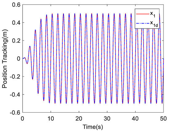
Figure 2. Tracking result of FOFA.

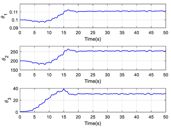
Figure 3. Parameter adaptation of FOFA.

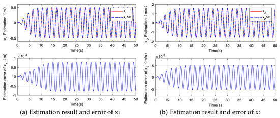
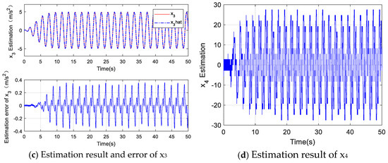
Figure 4. Estimation results of finite time observer.

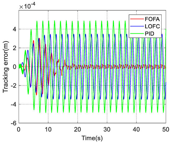
Figure 5. Comparison of position tracking error.

The estimation of the unknown system parameters of the FOFA controller is shown in Figure 3. It can be seen that the estimations of the parameters θ₁, θ₂ and θ₃ have converged effectively. In Figure 4, it can be seen that the estimated position value and actual position value are consistent well in (a), and the estimated values of the signal x₂ and x₃ and the unmodeled disturbances can also be accurately obtained in (b) and (c), which proves the effectiveness of the observer. The unmodeled disturbance term estimated by the observer is shown in (d). As shown in Figure 2 and Figure 5, the FOFA controller shows excellent tracking performance, and the magnitude of its steady-state tracking error is about 3 × 10⁻⁴ m at the maximum at the beginning and quickly converges to about 2.1 × 10⁻⁵ m. It can be seen that the tracking error of the FOFA controller is relatively large at the initial stage, but under the action of the parameter adaptation law and the finite time control, the estimated values of the unknown parameters of the system gradually converge, and the tracking error gradually decreases, which verifies the asymptotic tracking performance of the FOFA controller. In comparison, the amplitude of the steady-state tracking error of the LOFC controller is basically stable at about 3.5 × 10⁻⁴ m. The tracking error of the PID controller is maintained at about 4.9 × 10⁻⁴ m. Due to the large gain selected for the PID controller, the tracking error of PID controller produces slight chattering, which is not conducive to the stable operation of the actual system.

Case 2. The desired tracking command and the tracking result of FOFA is shown in Figure 6, namely 0.5sin(0.5 × πt)·(1−e^−0.05t) m.

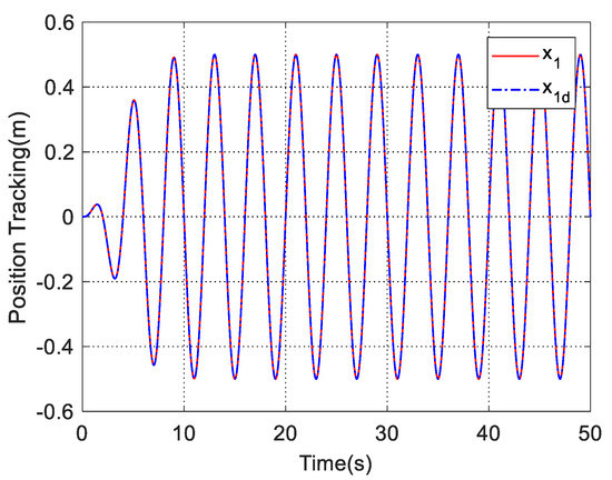
Figure 6. Tracking result of FOFA.

As shown in Figure 6 and Figure 7, the FOFA controller shows superior tracking performance, and the magnitude of its tracking error is about 1.4 × 10⁻⁴ m at the maximum at the beginning and quickly converges to about 3.1 × 10⁻⁵ m. In comparison, the magnitude of tracking error of LOFC is about 2.43 × 10⁻⁴ m at the maximum, and the amplitude of the steady-state tracking error of the LOFC controller in is stable at about 1.02 × 10⁻⁴ m. The tracking error of the PID controller in is maintained at about 5.28 × 10⁻⁴ m.

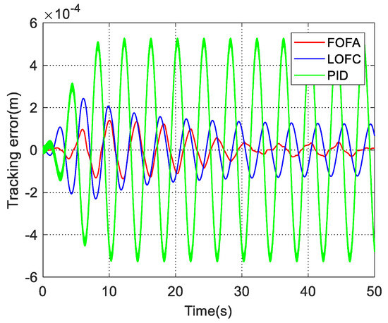
Figure 7. Comparison of position tracking error.

4.2. Comparison and Analysis of Point to Point Curve Tracking Performance

In order to further verify the tracking performance of the FOFA controller proposed in this paper, the desired tracking command is designed as point to point curve. the desired tracking command and the tracking result of FOFA are shown in Figure 8. The simulation results are shown in Figure 8 and Figure 9.

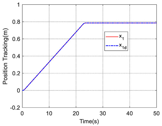
Figure 8. Tracking result of FOFA.

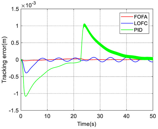
Figure 9. Comparison of position tracking error.

Figure 8 shows the tracking process and tracking error of the of the FOFA controller. Due to a sudden change in the expected instruction, it can be seen that the tracking error of the FOFA controller is about −3.6 × 10⁻⁵ m at the maximum, which is relatively large at the initial stage. The final tracking error stabilizes at 2.9 × 10⁻⁶ m. The tracking error of the LOFC controller is about −3.9 × 10⁻⁴ m at the maximum and the final tracking error of LOFC stabilizes at 6.7 × 10⁻⁵ m. It can be seen that slight chattering with an amplitude about 4 × 10⁻⁵ m is obtained in the final steady state by PID controller, due to the high-gain feedback selected, which is not conducive to the stable operation of the actual system. The LOFC controller takes advantage of the robustness of linear feedback control, and parameter adaptation that can estimate and compensate unknown system parameters, as well as Extended-State-Observer that attains feed-forward compensation for unmodeled and external disturbances in the system. Therefore, the transient and steady-state tracking performance of the LOFC controller is much better than the PID controller. The finite time control method combined with parameter adaption in FOFA controller can ensure that the system tracking error achieves finite time convergence through the analysis of Lyapunov function. While the control method used in LOFC controller is linear feedback method, which can only ensure that the system tracking error achieves a bounded stability. Therefore, the robustness of FOFA controller is stronger than that of LOFC controller. In addition, the finite time observer can achieve finite time convergence, while the ESO can only achieve exponential convergence, so the observation performance of the finite time observer is better than ESO. From Figure 9, it can be seen that although both controllers use parameter adaptation for feedforward compensation, the tracking performance of the FOFA controller is better than that of the LOFC controller.

5. Conclusions

In this paper, a finite-time output feedback control with parameter adaptation is proposed for hydraulic servo system. This control strategy takes into account the non-measured states, parametric uncertainties and unmodeled disturbances. Based on the output position signal, the finite-time Levant observer is first employed to estimate the unmeasured states and unmodeled disturbances, which can eliminate the impact of measurement noise and disturbances on control performance in a finite time. Then, based on a parameter adaptive law, the parametric uncertainties in the system can be much relieved, which can effectively reduce the high-gain feedback. In addition, in order to suppress the residual error of disturbances and further achieve excellent transient and steady-state tracking performance, a finite time output feedback super-twisting sliding mode controller has been presented. Through the stability analysis based on Lyapunov theory, it can be concluded that the developed controller has the finite-time stability. The comparative simulation results verify the effectiveness of the proposed control strategy. However, the proposed control method was only verified via numerical simulation. In the future, it is of great significance to further verify and testify the advantages of this new controller in practical experimental platform.

References

- Yao, J.; Deng, W. Active disturbance rejection adaptive control of hydraulic servo systems. IEEE Trans. Ind. Electron. 2017, 64, 6469–6477. [Google Scholar] [CrossRef]
- Deng, W.; Yao, J.; Wang, Y.; Yang, X.; Chen, J. Output feedback backstepping control of hydraulic actuators with valve dynamics compensation. Mech. Syst. Signal Process. 2021, 158, 107769. [Google Scholar] [CrossRef]
- Deng, W.; Yao, J. Extended-state-observer-based adaptive control of electrohydraulic servomechanisms without velocity measurement. IEEE/ASME Trans. Mechatron. 2020, 25, 1151–1161. [Google Scholar] [CrossRef]
- Merritt, H.E. Hydraulic Control Systems; Wiley: New York, NY, USA, 1967. [Google Scholar]
- Lyu, L.; Chen, Z.; Yao, B. Advanced Valves and Pump Coordinated Hydraulic Control Design to Simultaneously Achieve High Accuracy and High Efficiency. IEEE Trans. Control Syst. Technol. 2021, 29, 236–248. [Google Scholar] [CrossRef]
- Yao, J.; Deng, W.; Sun, W. Precision Motion Control for Electro-Hydraulic Servo Systems with Noise Alleviation: A Desired Compensation Adaptive Approach. IEEE/ASME Trans. Mechatron. 2017, 22, 1859–1868. [Google Scholar] [CrossRef]
- Plummer, A.R.; Vaughan, N.D. Robust Adaptive Control for Hydraulic Servosystems. J. Dyn. Syst. Meas. Control 1996, 118, 237–244. [Google Scholar] [CrossRef]
- Milić, V.; Šitum, Ž.; Essert, M. Robust position control synthesis of an electro-hydraulic servo system. ISA Trans. 2010, 49, 535–542. [Google Scholar] [CrossRef]
- Sun, W.; Gao, H.; Kaynak, O. Finite Frequency Control for Vehicle Active Suspension Systems. IEEE Trans. Control Syst. Technol. 2011, 19, 416–422. [Google Scholar] [CrossRef]
- Chen, H.; Liu, J.; Chen, G. Application of H∞ algorithm in hydraulic control system of loader. Int. Rev. Comput. Softw. 2011, 6, 1334–1338. [Google Scholar]
- Yao, J.; Deng, W.; Jiao, Z. RISE-Based Adaptive Control of Hydraulic Systems with Asymptotic Tracking. IEEE Trans. Autom. Sci. Eng. 2015, 14, 1–8. [Google Scholar] [CrossRef]
- Yao, J.; Jiao, Z.; Ma, D. Adaptive Robust Control of DC Motors with Extended State Observer. IEEE Trans. Ind. Electron. 2014, 61, 3630–3637. [Google Scholar] [CrossRef]
- Chen, Z.; Yao, B.; Wang, Q. Adaptive Robust Precision Motion Control of Linear Motors with Integrated Compensation of Nonlinearities and Bearing Flexible Modes. IEEE Trans. Ind. Inform. 2013, 9, 965–973. [Google Scholar] [CrossRef]
- Yao, B. Desired Compensation Adaptive Robust Control. J. Dyn. Syst. Meas. Control 2009, 131, 636–650. [Google Scholar] [CrossRef]
- Yao, B.; Al-Majed, M. High-performance robust motion control of machine tools: An adaptive robust control approach and comparative experiments. IEEE/ASME Trans. Mechatron. 1997, 2, 63–76. [Google Scholar]
- Na, J.; Chen, Q.; Ren, X.; Guo, Y. Adaptive Prescribed Performance Motion Control of Servo Mechanisms with Friction Compensation. IEEE Trans. Ind. Electron. 2013, 61, 486–494. [Google Scholar] [CrossRef]
- Xu, B.; Yang, C.; Shi, Z. Reinforcement Learning Output Feedback NN Control Using Deterministic Learning Technique. IEEE Trans. Neural Netw. Learn. Syst. 2014, 25, 635–641. [Google Scholar]
- Dahunsi, O.A.; Pedro, J.O.; Nyandoro, O.T. Neural network-based model predictive control of a servo-hydraulic vehicle suspension system. Int. J. Appl. Math. Comput. Sci. 2009, 1–6. [Google Scholar]
- Liu, Y.; Huang, P.; Zhang, F.; Zhao, Y. Distributed formation control using artificial potentials and neural network for constrained multiagent systems. IEEE Trans. Control Syst. Technol. 2020, 28, 697–704. [Google Scholar] [CrossRef]
- Cerman, O.; Husek, P. Adaptive fuzzy sliding mode control for electro-hydraulic servo mechanism. Expert Syst. Appl. 2012, 39, 10269–10277. [Google Scholar] [CrossRef]
- Ho, T.H.; Ahn, K. Speed Control of a Hydraulic Pressure Coupling Drive Using an Adaptive Fuzzy Sliding-Mode Control. IEEE/ASME Trans. Mechatron. 2012, 17, 976–986. [Google Scholar] [CrossRef]
- Yin, S.; Shi, P.; Yang, H. Adaptive fuzzy control of strict-feedback nonlinear time-delay systems with unmodeled dynamics. IEEE Trans. Cybern. 2016, 46, 1926–1938. [Google Scholar] [CrossRef]
- Yang, X.; Yao, J.; Deng, W. Output feedback adaptive super-twisting sliding mode control of hydraulic systems with disturbance compensation. ISA Trans. 2021, 109, 175–185. [Google Scholar] [CrossRef]
- Burton, J.A.; Zinober, A.S.I. Continuous approximation of vsc. Int. J. Syst. Sci. 1986, 17, 875–885. [Google Scholar] [CrossRef]
- Boiko, I.; Fridman, L.; Pisano, A.; Usai, E. A comprehensive analysis of chattering in second order sliding mode control systems. In Modern Sliding Mode Control Theory; Sringer: Berlin/Heidelberg, Germany, 2008. [Google Scholar]
- Levant, A. Homogeneity approach to high-order sliding mode design. Automatica 2005, 41, 823–830. [Google Scholar] [CrossRef]
- Levant, A. Sliding order and sliding accuracy in sliding mode control. Int. J. Control 1993, 58, 1247–1263. [Google Scholar] [CrossRef]
- Shtessel, Y.; Taleb, M.; Plestan, F. A novel adaptive-gain supertwisting sliding mode controller: Methodology and application. Automatica 2012, 48, 759–769. [Google Scholar] [CrossRef]
- Dorato, P. An Overview of Finite-Time Stability. In Current Trends in Nonlinear Systems and Control; Birkhäuser Boston: New York, NY, USA, 2006. [Google Scholar]
- Giorgio, B.; Alessandro, P.; Elisabetta, P.; Elio, U. A survey of applications of second-order sliding mode control to mechanical systems. Int. J. Control 2003, 76, 875–892. [Google Scholar]
- Liu, Y.; Zhang, F.; Huang, P.; Lu, Y. Fixed-time consensus tracking for second-order multiagent systems under disturbance. IEEE Trans. Syst. Man Cybern. Syst. 2021, 51, 4883–4894. [Google Scholar] [CrossRef]
- Utkin, V. On convergence time and disturbance rejection of super-twisting control. IEEE Trans. Autom. Control 2013, 58, 2013–2017. [Google Scholar] [CrossRef]
- Jinpeng, Y.; Peng, S.; Lin, Z. Finite-time command filtered backstepping control for a class of nonlinear systems. Automatica 2018, 92, 173–180. [Google Scholar]
- Levant, A. Robust exact differentiation via sliding mode technique. Automatica 1998, 34, 379–384. [Google Scholar] [CrossRef]
- Shtessel, Y.B.; Shkolnikov, I.A.; Levant, A. Smooth second-order sliding modes: Missile guidance application. Automatica 2007, 43, 1470–1476. [Google Scholar] [CrossRef]
- Feng, J.E.; Wu, Z.; Sun, J.B. Finite-time Control of Linear Singular Systems with Parametric Uncertainties and Disturbances. Acta Autom. Sin. 2005, 31, 634–637. [Google Scholar]
- Hong, Y.; Wang, J.; Cheng, D. Adaptive finite-time control of nonlinear systems with parametric uncertainty. IEEE Trans. Autom. Control 2006, 51, 858–862. [Google Scholar] [CrossRef]
- Yip, P.P.; Hedrick, J.K. Adaptive dynamic surface control: A simplified algorithm for adaptive backstepping control of nonlinear systems. Int. J. Control 1998, 71, 959–979. [Google Scholar] [CrossRef]
- Deng, W.; Yao, J.; Ma, D. Time varying input delay compensation for nonlinear systems with additive disturbance: An output feedback approach. Int. J. Robust Nonlinear Control 2018, 28, 31–52. [Google Scholar] [CrossRef]
- Na, J.; Li, Y.; Huang, Y.; Gao, G.; Chen, Q. Output feedback control of uncertain hydraulic servo systems. IEEE Trans. Ind. Electron. 2020, 67, 490–500. [Google Scholar] [CrossRef]
- Levant, A. Higher-order sliding modes, differentiation and output-feedback control. Int. J. Control 2003, 76, 924–941. [Google Scholar] [CrossRef]
- Yao, Z.; Yao, J.; Sun, W. Adaptive rise control of hydraulic systems with multilayer neural-networks. IEEE Trans. Ind. Electron. 2019, 66, 8638–8647. [Google Scholar] [CrossRef]
- Yao, B.; Bu, F.; Chiu, G.T.C. Non-linear adaptive robust control of electro-hydraulic systems driven by double-rod actuators. Int. J. Control 2001, 74, 761–775. [Google Scholar] [CrossRef]
- Deng, W.; Yao, J. Asymptotic tracking control of mechanical servosystems with mismatched uncertainties. IEEE/ASME Trans. Mechatron. 2021, 26, 2204–2214. [Google Scholar] [CrossRef]
Publisher’s Note: MDPI stays neutral with regard to jurisdictional claims in published maps and institutional affiliations. |
© 2021 by the authors. Licensee MDPI, Basel, Switzerland. This article is an open access article distributed under the terms and conditions of the Creative Commons Attribution (CC BY) license (https://creativecommons.org/licenses/by/4.0/).