Semi-Supervised Gearbox Anomaly Detection Under Variable Operating Conditions

Abstract

Feature distributions shift under variable-speed gearbox operation, which can cause a model trained only on healthy samples to misclassify normal operating changes as anomalies. A semi-supervised anomaly detection method is proposed in this study. Using healthy data, the method first fits speed-dependent trends for the selected time- and frequency-domain statistics, and the deviations from these trends form the statistical residuals. Computed order tracking then converts the vibration signal to the angular domain, where five mechanism features describe meshing energy, harmonic structure, sideband modulation, and order-spectrum entropy. Removing the corresponding healthy speed trends yields the mechanism residuals. Robust Bounded Health-Consistency Weighting (RB-HCW) weights these residuals according to their variability in healthy data before they are fused with the statistical residuals and modeled by Deep Support Vector Data Description (DeepSVDD). The Sequential Bayesian Queue-Based Alarm (SBQA) module then confirms whether abnormal decisions persist across successive windows. Across the four fault types under the two separately modeled load conditions, the proposed method achieved macro-averaged true positive rate (TPR), accuracy (ACC), and F1-score values of 93.31%, 92.58%, and 94.02%, respectively.

1. Introduction

Gearboxes transmit power, alter rotational speed, and regulate torque in mechanical drivetrains. They are widely used in aerospace systems, energy equipment, and rail transportation [1,2,3,4]. During long-term operation, gears and bearings are repeatedly exposed to alternating loads, meshing impacts, and structural coupling, which may lead to pitting, missing or broken teeth, and compound gear–bearing damage. Such damage reduces transmission accuracy and efficiency and, in severe cases, can cause unplanned shutdowns or safety incidents. Feng and Zhang [5] proposed a hierarchical attention-guided data–knowledge fusion network that combines prior gearbox fault features with deep representations of monitoring data for few-shot diagnosis. Wang and Zhao [6] addressed a related multi-task problem with an attention-guided graph convolutional network that jointly estimates fault type and severity. For motor-current analysis, Chai and Xu [7] combined high-order multi-synchrosqueezing with an instantaneous-frequency polar view to resolve frequency modulation synchronized with faulty-gear meshing. Seo and Yun [8] used reduced-Lagrangian pseudo-labels to train a supervised classifier on otherwise unlabeled vibration signals. Kumar et al. [9] combined variational mode decomposition with a convolutional neural network for fault identification in a direct-shift gearbox. These studies demonstrate the diagnostic value of vibration and motor-current signals for assessing gearbox condition. Detecting departures from healthy behavior is, therefore, important for safe operation and predictive maintenance.

Industrial machines routinely accelerate, decelerate, and operate with speed fluctuations. As speed changes, meshing-frequency components move continuously along the frequency axis, causing spectral smearing and energy spreading. The excitation intensity and structural response also change, so statistics such as root mean square, energy, and peak-to-peak amplitude vary with the operating condition [10]. Urbanek et al. [11] studied instantaneous-speed estimation under large speed fluctuations to reduce their effect on spectral analysis. Fyfe and Munck [12] examined the error sources and applicability of computed order tracking. Order tracking maps a time-domain signal to the angular domain, fixing shaft-synchronous components at their corresponding orders. Nevertheless, feature amplitudes and statistical distributions remain affected by changes in speed, load, and transmission path.

Research on speed-induced distribution shift has followed two main directions: modeling healthy operating trends and incorporating mechanism information. Song et al. [13] fitted the normal relationship between statistical features and speed using healthy data, then used residuals from the fitted trend for anomaly detection. This reduced interference from speed-related components. Li et al. [14] determined fault characteristic frequencies from gearbox geometry and kinematics, used order analysis to obtain speed-stable characteristic orders, and combined time–frequency and order information in contrastive learning. Healthy-trend residuals measure departures from normal operating behavior, whereas mechanism priors provide a common physical reference across speed windows. The two forms of information are complementary.

Deep learning has also been used for intelligent diagnosis and anomaly detection under variable operating conditions. Zhao et al. [15] reduced inter-condition distribution differences using adaptive intraclass and interclass convolutions. Hu et al. [16] used a mutual-information constraint to separate condition-related and state-related information. Zhou et al. [17] combined convolutional layers with a Transformer to obtain stable features under time-varying conditions. Xu et al. [18] used clustering-guided contrastive learning for operating-condition recognition and anomaly representation. Li et al. [19] improved cross-condition diagnosis through knowledge mapping and adversarial domain adaptation. Although these methods can model nonlinear relationships, they generally require substantial training data, operating-condition labels, or source-domain fault samples, and their training and parameter selection are relatively complex. Li et al. [20] incorporated fault-spectrum knowledge into zero-shot contrastive learning, showing that mechanism knowledge can partly offset the scarcity of fault samples. A simpler model that retains physical interpretability, however, remains desirable.

Fault samples are often scarce in industrial settings. Critical equipment is usually serviced before a fault progresses far enough to yield a complete degradation record. Fault severity, load, and propagation path also vary, so a limited set of examples cannot cover all abnormal patterns encountered in service. Modeling the healthy state and treating samples outside its distribution as anomalous is therefore better aligned with the available data [21,22]. Tax and Duin [23] introduced support vector data description, which represents one-class data by a compact hypersphere. Ruff et al. [24] used a neural network to learn a compact nonlinear representation of healthy samples, leading to DeepSVDD. Peng et al. [25] added reconstruction and an adaptive threshold to deep one-class modeling. These approaches reduce dependence on fault labels, but most assume that training and monitoring data follow similar distributions. When speed shifts healthy features, normal operating changes may be labeled as anomalies. A single-window alarm is also susceptible to transient impacts and occasional noise.

Three issues remain in variable-speed gearbox anomaly detection. First, statistical residuals suppress speed trends but do not indicate whether a change occurs at physically meaningful locations such as meshing orders, harmonics, or sidebands. Second, mechanism features differ in their healthy-state variability. Equal weighting can, therefore, allow an unstable dimension to dominate the distance measure. Third, window-by-window decisions lack temporal confirmation, so a few isolated threshold crossings can trigger unnecessary alarms. A healthy-data framework should, therefore, account for operating trends, gearbox mechanisms, feature reliability, and confirmation across consecutive windows.

To address these issues, the proposed framework forms speed-conditioned residuals in parallel statistical and order-domain branches, weights the mechanism residuals according to their variability under healthy operation, and confirms whether window-level abnormal decisions persist over time. The main contributions are summarized as follows:

(1)

A dual-branch speed-conditioned residual representation is developed for variable-speed gearbox monitoring. Healthy speed trends are fitted separately for strongly speed-dependent statistical features and five order-domain mechanism features that describe meshing energy, harmonic structure, sideband modulation, and overall spectral complexity. Residuals from the two branches suppress normal speed-dependent variations while retaining complementary information about departures from healthy vibration behavior and gear-meshing structure;

(2)

The proposed RB-HCW method stabilizes information fusion. It uses the median absolute deviation of each healthy residual as a robust measure of normal variability, then applies weight clipping and mean normalization to prevent unstable feature dimensions from dominating the joint representation. The weighted residuals are fused with the statistical residuals before DeepSVDD learns the healthy feature distribution;

(3)

For continuous monitoring, SBQA incorporates Bayesian sequence confirmation into window-level anomaly detection. Successive binary decisions are stored in a first-in, first-out queue, and a Beta posterior probability assesses whether the recent anomaly evidence is persistent. An alarm is issued only after the queue reaches its specified length and the posterior probability exceeds the confirmation threshold. This requirement limits the influence of isolated threshold crossings on the final monitoring result.

The remainder of this paper is organized as follows. Section 2 describes healthy-domain modeling with DeepSVDD, speed-residual statistical features, mechanism residuals, RB-HCW fusion, and SBQA confirmation. Section 3 presents the dataset, experimental setup, evaluation metrics, comparison and ablation studies, and parameter sensitivity analysis. Section 4 concludes the paper and outlines future work.

2. Methodology

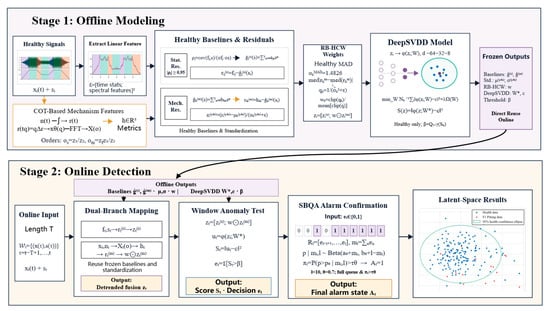
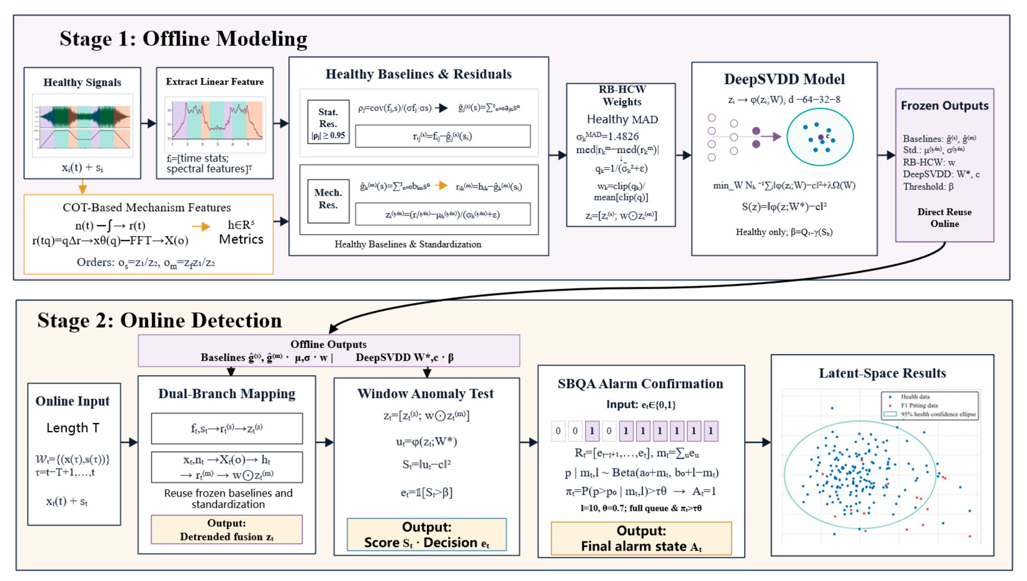
The proposed framework is shown in Figure 1 and consists of feature construction, anomaly detection, and alarm confirmation. In the first stage, vibration and speed signals are collected from the target gearbox. Time- and frequency-domain statistics and order-domain mechanism features are extracted, and healthy-trend models are used to form speed-residual statistics and mechanism residuals. In the second stage, RB-HCW weights the mechanism residuals, which are fused with the statistical residuals. DeepSVDD then learns the healthy feature distribution and produces a continuous anomaly score. In the third stage, a threshold gives a single-window decision, and SBQA confirms decisions over successive windows to reduce false alarms caused by transient impacts and external disturbances.

Figure 1. Workflow of the proposed method.

2.1. DeepSVDD-Based Healthy-Domain Modeling

Support Vector Data Description (SVDD), introduced by Tax and Duin [23], is a boundary learning method for one-class data. Using only healthy samples, SVDD constructs a hypersphere that contains most normal observations while allowing a small number to lie outside the boundary through slack variables. Let the fused feature of the ith healthy sample be Z_i with dimension d, and let the total number of healthy samples be N_h, where i = 1, …, N_h. The soft-boundary optimization problem is:

$$\begin{array}{c}\underset{R,c,\xi }{\mathrm{m}\mathrm{i}\mathrm{n}}{R}^2+{\displaystyle \frac{1}{\nu N_h}}{\displaystyle \sum _{i=1}^{N_h}}{\xi }_i,\\ \mathrm{s}.\mathrm{t}. {‖\psi \left(z_i\right)-c‖}_2^2\le R^2+{\xi }_i, {\xi }_i\ge 0\end{array}$$

(1)

where R and c are the radius and center of the hypersphere, respectively. Here, ψ(·) is the feature mapping, ξ_i is the slack variable associated with the ith healthy sample, and ν controls the compactness of the hypersphere and the penalty for samples outside it. By minimizing both the radius and the boundary violations under the stated constraints, the optimization places most healthy samples inside the hypersphere and defines the healthy boundary. For a d-dimensional test sample Z, the decision function is:

$$g\left(z\right)={‖\psi \left(z\right)-c‖}_2^2-R^2$$

(2)

A sample is classified as anomalous when g(z) > 0, indicating that it lies outside the healthy boundary. Conventional SVDD relies on a predefined kernel or handcrafted feature mapping. Its performance can, therefore, be sensitive to the kernel and its parameters, and it may not represent complex nonlinear data well. Ruff et al. [24] addressed this limitation by introducing a deep neural network into SVDD, resulting in Deep Support Vector Data Description (DeepSVDD). A network Φ(·, W), parameterized by W, replaces the fixed mapping and projects the input into a latent space. Constraining the healthy representations toward a common center yields a compact description of the healthy distribution.

Following this principle, DeepSVDD is used to learn a healthy boundary for the fused features. The feature-mapping network is a bias-free multilayer feedforward network whose input dimension matches the fused feature vector. Before training, healthy samples are mapped using the initial parameters W₀, and the mean latent representation initializes the healthy center c:

$$c={\displaystyle \frac{1}{N_h}}{{\displaystyle \sum }}_{i=1}^{N_h}\varphi \left(z_i;W_0\right)$$

(3)

After the initial center is obtained from Equation (3), any component too close to zero is replaced by a small nonzero value to prevent the network from collapsing to the zero vector. The center c is then fixed, and the network parameters are learned by minimizing the mean squared distance between the healthy latent representations and c:

$${\mathcal{L}}_{\mathrm{S}\mathrm{V}\mathrm{D}\mathrm{D}}=N_h^{-1}{\displaystyle \sum _{i=1}^{N_h}}{‖\phi \left(z_i,W\right)-c‖}_2^2+\lambda \Omega \left(W\right)$$

(4)

where W denotes the network parameters, Ω(W) is the regularization term, and λ ≥ 0 is the regularization coefficient. Minimizing Equation (4) gives the optimized parameters W*. Only healthy samples are used in training, with the objective of concentrating their latent representations around the healthy center.

After training, the feature vector Z from any test window is mapped by the trained network. The squared Euclidean distance between its latent representation and the healthy center is used as the continuous anomaly score:

$$S\left(z\right)={‖\phi \left(z,W\right)-c‖}_2^2$$

(5)

A larger anomaly score S(z) indicates a greater distance from the healthy center and a stronger departure from the healthy distribution. After training, anomaly scores are calculated for all healthy training samples. Given a preset anomaly proportion γ, the 100(1 − γ)th percentile of these scores is used as the detection threshold β:

$$\mathsf{\beta }=\mathrm{Percentile}\left({\left\{S\left(z_i\right)\right\}}_{i=1}^{N_h},100\left(1-\mathsf{\gamma }\right)\right)$$

(6)

where Percentile(·) denotes the percentile function and γ ∈ (0, 1) is the preset anomaly proportion. A test window is classified as anomalous when S(z) > β.

2.2. Speed-Residual Statistical Features

DeepSVDD depends on input features that represent the healthy state consistently. Under variable-speed operation, however, features change with rotational speed, and even healthy samples can follow different distributions in different speed ranges. Reference [13] represented each feature as the sum of a speed-dependent trend and a residual, fitting the normal feature–speed relationship from healthy samples. The difference between the observation and its trend prediction forms a residual feature. This procedure suppresses speed-induced drift and improves consistency across speed ranges. The residuals are used here as inputs to DeepSVDD.

The continuously acquired vibration signal is divided into sliding windows, and the mean speed is calculated for each segment. In addition to conventional time-domain features, nine frequency-domain features are extracted: spectral decrease, spectral skewness, spectral distance, spectral spread, spectral kurtosis, spectral entropy, median frequency, spectral centroid, and power bandwidth [26]. The time-domain features describe amplitude, dispersion, distribution shape, and local variation, whereas the frequency-domain features characterize spectral energy, frequency location, and spectral complexity. Table 1 lists the time-domain features, while definitions of the nine frequency-domain features are provided in Ref. [26]. The resulting statistical feature vectors and their paired speed values are used for correlation analysis and residual modeling.

Table 1. Time-domain features used in this study.

Definition
Mean	${\displaystyle \frac{1}{\mathrm{N}}}{\displaystyle {\displaystyle \sum }_{\mathrm{i}=1}^{\mathrm{N}}}{\mathrm{x}}_{\mathrm{i}}$	Variance	${\displaystyle \frac{1}{N}}{\displaystyle {\displaystyle \sum }_{i=1}^N}{\left(x_i-{\mu }_x\right)}^2$
Standard deviation	$\sqrt{{\displaystyle \frac{1}{\mathrm{N}}}{\displaystyle {\displaystyle \sum }_{\mathrm{i}=1}^{\mathrm{N}}}{\left({\mathrm{x}}_{\mathrm{i}}-{\mathrm{\mu }}_{\mathrm{x}}\right)}^2}$	Skewness	${\displaystyle \frac{N^{-1}{{\displaystyle \sum }}_{i=1}^N{\left(x_i-{\mu }_x\right)}^3}{{\sigma }_x^3}}$
Kurtosis	${\displaystyle \frac{N^{-1}{{\displaystyle \sum }}_{i=1}^N{\left(x_i-{\mu }_x\right)}^4}{{\sigma }_x^4}}$	Root mean square	$\sqrt{{\displaystyle \frac{1}{N}}{\displaystyle {\displaystyle \sum }_{i=1}^N}{x}_i^2}$
Mean difference	${\displaystyle \frac{1}{N-1}}{\displaystyle {\displaystyle \sum }_{i=1}^{N-1}}\left(x_{i+1}-x_i\right)$	Mean absolute deviation	${\displaystyle \frac{1}{N}}{\displaystyle {\displaystyle \sum }_{i=1}^N}\left|x_i-{\mu }_x\right|$
Mean absolute difference	${\displaystyle \frac{1}{N-1}}{\displaystyle {\displaystyle \sum }_{i=1}^{N-1}}\left|x_{i+1}-x_i\right|$	Mean power	${\displaystyle \frac{1}{N}}{\displaystyle {\displaystyle \sum }_{i=1}^N}{x}_i^2$
Area under the curve	${\displaystyle \frac{1}{2f_s}}{\displaystyle {\displaystyle \sum }_{i=1}^{N-1}}\left|x_{i+1}+x_i\right|$	Absolute energy	${\displaystyle {\displaystyle \sum }_{i=1}^N}{x}_i^2$
Maximum	${\max }_i\left(x_i\right)$	Minimum	${\min }_i\left(x_i\right)$
Peak-to-peak value	$x_{\max }-x_{\min }$	Median	$\mathrm{median}\left(x_i\right)$
Median absolute difference	$\mathrm{median}\left(\left|x_{i+1}-x_i\right|\right)$	Time centroid	${\displaystyle \frac{{{\displaystyle \sum }}_{i=0}^{N-1}\left(i/f_s\right){\left|x_i\right|}^2}{{{\displaystyle \sum }}_{i=0}^{N-1}{\left|x_i\right|}^2}}$
Interquartile range	$Q_{0.75}\left(x\right)-Q_{0.25}\left(x\right)$	Median difference	$\mathrm{median}\left(x_{i+1}-x_i\right)$
Median absolute deviation	$\mathrm{median}\left(\left|x_i-x_{\mathrm{med}}\right|\right)$	Time-domain entropy	$-{\displaystyle \frac{{{\displaystyle \sum }}_{j=1}^J{p}_j{\log }_2{p}_j}{{\log }_{2}N}}$

The statistical features do not respond equally to speed. For a weakly correlated feature, a direct trend fit may not provide a stable healthy baseline. Features that are strongly affected by speed are, therefore, selected before residual modeling. Following [13], the Pearson correlation coefficient (PCC) [27] measures the linear correlation between the jth statistical feature and the mean window speed:

$${\mathsf{\rho }}_{\mathrm{j}}={\displaystyle \frac{{{\displaystyle \sum }}_{\mathrm{i}=1}^{{\mathrm{N}}_{\mathrm{h}}}\left({\mathrm{f}}_{\mathrm{ij}}-\overline{{\mathrm{f}}_{\mathrm{j}}}\right)\left({\mathrm{s}}_{\mathrm{i}}-\overline{\mathrm{s}}\right)}{\sqrt{{{\displaystyle \sum }}_{\mathrm{i}=1}^{{\mathrm{N}}_{\mathrm{h}}}{\left({\mathrm{f}}_{\mathrm{ij}}-\overline{{\mathrm{f}}_{\mathrm{j}}}\right)}^2}\sqrt{{{\displaystyle \sum }}_{\mathrm{i}=1}^{{\mathrm{N}}_{\mathrm{h}}}{\left({\mathrm{s}}_{\mathrm{i}}-\overline{\mathrm{s}}\right)}^2}}}$$

(7)

where f_ij is the jth statistical feature of the ith healthy window, $\overline{f_j}$ and $\overline{s}$ are the mean feature value and mean speed over the healthy samples, respectively, and ρ_j ∈ [−1, 1]. As |ρ_j| approaches 1, the linear relationship with speed becomes stronger. The selection criterion |ρ_j| ≥ 0.95 retains both strongly positive and strongly negative correlations for subsequent trend fitting.

After feature selection, healthy samples are used to establish the normal speed trend of each retained feature. Song et al. [13] compared several functional forms and used a cubic polynomial for the healthy feature–speed relationship. The same trend model is adopted here for the jth selected statistical feature:

$${\hat{\mathrm{g}}}_{\mathrm{j}}\left(\mathrm{s}\right)={\mathrm{a}}_{\mathrm{j}0}+{\mathrm{a}}_{\mathrm{j}1}\mathrm{s}+{\mathrm{a}}_{\mathrm{j}2}{\mathrm{s}}^2+{\mathrm{a}}_{\mathrm{j}3}{\mathrm{s}}^3$$

(8)

where a_j0 through a_j3 are least-squares regression coefficients estimated from healthy samples, and ĝ_j(s_i) is the healthy-trend prediction for the ith window at speed s_i. Subtracting this prediction from the observed feature suppresses speed-induced variation. The speed-residual statistical feature vector of the ith window is:

$$r_{\mathrm{i}}^{\left(\mathrm{s}\right)}={\left[{\mathrm{f}}_{\mathrm{i}1}-{\hat{\mathrm{g}}}_1\left({\mathrm{s}}_{\mathrm{i}}\right),\dots ,{\mathrm{f}}_{\mathrm{iJ}}-{\hat{\mathrm{g}}}_{\mathrm{J}}\left({\mathrm{s}}_{\mathrm{i}}\right)\right]}^{\mathrm{T}}$$

(9)

2.3. Order-Domain Mechanism Residuals

Speed-residual statistics quantify departures from healthy speed trends but do not locate the underlying physical change. Gear-surface damage alters meshing impacts and produces responses near the meshing frequency, its harmonics, and sidebands spaced by the shaft rotational frequency [28]. The mechanism branch, therefore, proceeds in three steps. First, equal-angle resampling produces an order spectrum that is less sensitive to speed. Second, gearbox geometry defines mechanism indicators, and their residuals from healthy speed trends are calculated. Third, the mechanism residuals are weighted according to their healthy-state consistency, with bounds applied to prevent excessive weights, and then fused with the statistical residuals.

As the speed changes, a meshing-frequency component moves along the frequency axis, so comparing spectra from different windows may mistake peak displacement for a state change. Computed order tracking [12] addresses this problem by mapping the time-domain signal to the angular domain. An order is the ratio of a vibration frequency to the reference-shaft rotational frequency. A shaft-synchronous component, therefore, remains near a fixed position on the order axis. The cumulative revolutions within a window are first calculated from the synchronized speed, and the vibration signal is then interpolated at uniform angular increments:

$$\mathrm{r}\left(\mathrm{t}\right)={{\displaystyle \int }}_0^{\mathrm{t}}{\displaystyle \frac{\mathrm{n}\left(\mathsf{\tau }\right)}{60}}\mathrm{d}\mathsf{\tau },{\mathrm{x}}_{\mathsf{\theta }}\left(\mathrm{q}\right)=\mathrm{x}\left({\mathrm{t}}_{\mathrm{q}}\right),\mathrm{r}\left({\mathrm{t}}_{\mathrm{q}}\right)=\mathrm{q}\mathsf{\Delta }\mathrm{r}$$

(10)

where n(t) is the instantaneous reference-shaft speed in rpm, r(t) is the cumulative number of revolutions from the start of the window to time t, Δr is the revolution increment between adjacent angular samples, t_q is the time corresponding to the qth equal-angle sample, and x_θ(q) is the resampled vibration sequence. This procedure divides each revolution into equal angular increments and keeps shaft-synchronous components at fixed positions on the order axis. After removing the mean of x_θ(q), a fast Fourier transform gives the order spectrum X(o). The characteristic orders are determined from the gearbox tooth counts:

$$\begin{array}{ccc}& {\mathrm{o}}_{\mathrm{s}}={\displaystyle \frac{{\mathrm{z}}_1}{{\mathrm{z}}_2}},{\mathrm{o}}_{\mathrm{m}}={\mathrm{z}}_{\mathrm{f}}{\displaystyle \frac{{\mathrm{z}}_1}{{\mathrm{z}}_2}}& \end{array}$$

(11)

In Equation (11), z₁ and z₂ are the tooth counts of the input-shaft gear and the large intermediate-shaft gear, respectively, and z_f is the tooth count of the target gear. The intermediate-shaft rotational order is o_s, and the target-gear meshing order is o_m. These orders depend on the tooth counts and transmission ratio, so their theoretical positions do not vary with speed. They provide a common reference for feature extraction from different speed windows. Five mechanism features are constructed around o_m, its second harmonic 2o_m, and the upper and lower sidebands spaced by o_s. Together, they describe meshing energy, harmonic relationships, sideband modulation, and the overall spectral distribution.

The statistical and mechanism branches are aligned at the window level. Each continuous record is first divided into 9126-sample candidate windows with 50% overlap for statistical feature extraction. The center time of each candidate window anchors a mechanism-analysis segment containing two complete revolutions on either side, giving a fixed length of four revolutions. Each segment is resampled to 2048 equally spaced angular samples before its order spectrum is calculated. Candidates near the record boundaries are removed when a complete four-revolution segment is unavailable, and the remaining indices are used for both feature branches and all comparison methods. Because every segment contains four complete revolutions, the theoretical order resolution is 0.25 order, below the sideband spacing of 0.305 order.

Meshing-order energy ratio h₁: This feature is the energy near the target meshing order divided by the total order-spectrum energy. It measures the relative concentration of the principal meshing component and is defined as:

$${\mathrm{h}}_1={\displaystyle \frac{\mathrm{E}\left({\mathrm{o}}_{\mathrm{m}}\right)}{{\mathrm{E}}_{\mathrm{T}}}}$$

(12)

Second-to-first harmonic ratio h₂: This feature compares the energy at twice the meshing order with the energy at the fundamental meshing order. It characterizes distortion of the meshing waveform and its harmonic structure:

$${\mathrm{h}}_2={\displaystyle \frac{\mathrm{E}\left(2{\mathrm{o}}_{\mathrm{m}}\right)}{\mathrm{E}\left({\mathrm{o}}_{\mathrm{m}}\right)+\mathsf{\epsilon }}}$$

(13)

Sideband-to-carrier ratio h₃: When a localized gear defect enters the meshing region periodically, it amplitude-modulates the meshing carrier and produces sidebands around o_m at intervals of o_s. A larger ratio generally indicates stronger periodic impacts or load fluctuations and is, therefore, sensitive to localized tooth-surface damage:

$${\mathrm{h}}_3={\displaystyle \frac{\mathrm{E}\left({\mathrm{o}}_{\mathrm{m}}-{\mathrm{o}}_{\mathrm{s}}\right)+\mathrm{E}\left({\mathrm{o}}_{\mathrm{m}}+{\mathrm{o}}_{\mathrm{s}}\right)}{\mathrm{E}\left({\mathrm{o}}_{\mathrm{m}}\right)+\mathsf{\epsilon }}}$$

(14)

Sideband asymmetry h₄: Feature h₃ measures the combined strength of the two sidebands but does not distinguish whether the energy is concentrated above or below the carrier. Sideband asymmetry captures differences in modulation structure and transmission path, allowing windows with similar total sideband energy but different distributions to be distinguished:

$${\mathrm{h}}_4={\displaystyle \frac{\mathrm{E}\left({\mathrm{o}}_{\mathrm{m}}+{\mathrm{o}}_{\mathrm{s}}\right)-\mathrm{E}\left({\mathrm{o}}_{\mathrm{m}}-{\mathrm{o}}_{\mathrm{s}}\right)}{\mathrm{E}\left({\mathrm{o}}_{\mathrm{m}}+{\mathrm{o}}_{\mathrm{s}}\right)+\mathrm{E}\left({\mathrm{o}}_{\mathrm{m}}-{\mathrm{o}}_{\mathrm{s}}\right)+\mathsf{\epsilon }}}$$

(15)

Normalized order-spectrum entropy h₅: This feature measures the overall dispersion of energy in the order spectrum. It complements the four local-order features by capturing the global spectral changes not fully represented by a single meshing order, harmonic, or sideband:

$${\mathrm{h}}_5=-{\displaystyle \frac{{{\displaystyle \sum }}_{\mathrm{k}=1}^{\mathrm{N}}{\mathrm{p}}_{\mathrm{k}}\ln \left({\mathrm{p}}_{\mathrm{k}}+\mathsf{\epsilon }\right)}{\mathrm{lnN}}},{\mathrm{p}}_{\mathrm{k}}={\displaystyle \frac{{\mathrm{P}}_{\mathrm{k}}}{{\mathrm{E}}_{\mathrm{T}}}}$$

(16)

Taken together, the five indicators describe complementary changes in the order spectrum. The meshing-order energy ratio measures how strongly energy is concentrated near the target meshing order, whereas the second-to-first harmonic ratio reflects waveform distortion and redistribution between the first two harmonics. The sideband-to-carrier ratio measures periodic modulation strength, and sideband asymmetry describes how that modulation energy is distributed on either side of the carrier. Order-spectrum entropy adds a global measure of spectral dispersion and complexity. The resulting feature group, therefore, combines local meshing and modulation information with the overall spectral distribution. Ratios and normalization reduce sensitivity to overall amplitude, but healthy values may still drift with speed because of the speed-estimation error at low speeds, keyphasor interpolation error, finite-data effects, and the vibration transmission path. A separate cubic healthy speed trend is fitted to each indicator, and the mechanism residual is defined as its deviation from that trend:

$${\mathrm{r}}_{\mathrm{ik}}^{\left(\mathrm{m}\right)}={\mathrm{h}}_{\mathrm{ik}}-{\hat{\mathrm{g}}}_{\mathrm{k}}^{\left(\mathrm{m}\right)}\left({\mathrm{s}}_{\mathrm{i}}\right),\mathrm{k}=1,\dots ,\mathrm{K}$$

(17)

where h_ik is the kth mechanism indicator from the ith window, k = 1, …, K, and K = 5, ĝ_k^(m)(s_i) is the healthy-trend prediction at speed s_i, and r_ik^(m) is the corresponding mechanism residual. The trend models for the statistical and mechanism branches are estimated during training and remain fixed during monitoring. Each branch is standardized using parameters estimated from the healthy training set to remove scale differences:

$${\mathrm{z}}_{\mathrm{ik}}^{\left(\mathrm{m}\right)}={\displaystyle \frac{{\mathrm{r}}_{\mathrm{ik}}^{\left(\mathrm{m}\right)}-{\mathsf{\mu }}_{\mathrm{k}}^{\left(\mathrm{m}\right)}}{{\mathsf{\sigma }}_{\mathrm{k}}^{\left(\mathrm{m}\right)}+ϵ}},{\mathrm{z}}_{\mathrm{ij}}^{\left(\mathrm{s}\right)}={\displaystyle \frac{{\mathrm{r}}_{\mathrm{ij}}^{\left(\mathrm{s}\right)}-{\mathsf{\mu }}_{\mathrm{j}}^{\left(\mathrm{s}\right)}}{{\mathsf{\sigma }}_{\mathrm{j}}^{\left(\mathrm{s}\right)}+ϵ}}$$

(18)

2.4. RB-HCW Weighting and Feature Fusion

Standardization aligns feature means and variances but does not make every mechanism dimension equally stable in the healthy state. Because the dimensions describe different spectral structures, their standardized residuals can still differ in concentration and tail behavior. If all dimensions receive equal weight in a distance-based one-class model, an unstable healthy feature may have an excessive effect on the sample distance and increase false alarms. RB-HCW is, therefore, applied after branch-wise standardization. It uses only healthy training samples to estimate the stability of each mechanism dimension and adjusts its contribution in a robust, bounded manner. For the kth mechanism residual, the median absolute deviation (MAD) is:

$${\sigma }_k^{\mathrm{MAD}}=1.4826{\mathrm{median}}_i\left(\left|r_{ik}^{\left(m\right)}-{\mathrm{median}}_u\left(r_{uk}^{\left(m\right)}\right)\right|\right)$$

(19)

where σ_kᴹᴬᴰ is the MAD scale of the kth mechanism residual. The factor 1.4826 provides the normal-consistency correction, allowing the scaled MAD to estimate the standard deviation for normally distributed residuals. Unlike the conventional standard deviation, MAD is resistant to a small number of extreme residuals and, therefore, describes the concentration of the main body of healthy samples more robustly.

For a highly concentrated mechanism residual, the MAD may be zero or nearly zero. A small positive lower bound is imposed to avoid numerical instability when the reciprocal is taken:

$${\tilde{\mathsf{\sigma }}}_{\mathrm{k}}=\max \left({\mathsf{\sigma }}_{\mathrm{k}}^{\mathrm{MAD}},\mathsf{\epsilon }\right)$$

(20)

where $\epsilon >0$ is a small positive constant that prevents a zero scale estimate. A smaller ${\tilde{\sigma }}_k$ from Equation (20) indicates that the kth mechanism residual is more concentrated and consistent across healthy windows. The weights are assigned inversely to this variability. A smaller robust scale receives a larger weight, and a larger scale receives a smaller one. The initial weights are then normalized to have a mean of 1 so that the overall scale of the mechanism branch remains approximately unchanged:

$${\mathrm{q}}_{\mathrm{k}}={\displaystyle \frac{1}{{\tilde{\mathsf{\sigma }}}_{\mathrm{k}}^2+ϵ}},{\mathrm{w}}_{\mathrm{k}}^{\left(0\right)}={\displaystyle \frac{{\mathrm{q}}_{\mathrm{k}}}{{\mathrm{K}}^{-1}{{\displaystyle \sum }}_{\mathrm{u}=1}^{\mathrm{K}}{\mathrm{q}}_{\mathrm{u}}}}$$

(21)

where q_k is the health-consistency score of the kth mechanism residual and w_k⁽⁰⁾ is its initial weight. The inverse-square relationship emphasizes features with low healthy-state variability and good repeatability, but it can overconcentrate the weights when ${\tilde{\sigma }}_k$ is very small. To prevent one feature from dominating the fused space, the initial weights are clipped to [K⁻¹ᐟ², K¹ᐟ²] according to the number of mechanism features K and are then renormalized to the unit mean:

$${\mathrm{w}}_{\mathrm{k}}={\displaystyle \frac{\mathrm{clip}\left({\mathrm{w}}_{\mathrm{k}}^0,{\mathrm{K}}^{-\frac{1}{2}},{\mathrm{K}}^{\frac{1}{2}}\right)}{{\mathrm{K}}^{-1}{\displaystyle {\displaystyle \sum _{\mathrm{u}=1}^{\mathrm{K}}\mathrm{clip}\left({\mathrm{w}}_{\mathrm{u}}^0,{\mathrm{K}}^{-\frac{1}{2}},{\mathrm{K}}^{\frac{1}{2}}\right)}}}},\mathrm{clip}\left(\mathrm{a},\mathrm{l},\mathrm{u}\right)=\min \left\{\max \left(\mathrm{a},\mathrm{l}\right),\mathrm{u}\right\}$$

(22)

where w_k is the final weight of the kth mechanism indicator. Clipping retains information from every mechanism dimension, prevents an unusually small scale from producing an excessive weight, and keeps the mean weight of the mechanism branch equal to 1. The weights are estimated from the unstandardized healthy mechanism residuals and applied to the standardized mechanism vector. The statistical residuals and weighted mechanism residuals are finally concatenated as the DeepSVDD input:

$${\mathrm{z}}_{\mathrm{i}}={\left[{\left({\mathrm{z}}_{\mathrm{i}}^{\left(\mathrm{s}\right)}\right)}^{\mathrm{T}},{\left(\mathrm{w}\odot {\mathrm{z}}_{\mathrm{i}}^{\left(\mathrm{m}\right)}\right)}^{\mathrm{T}}\right]}^{\mathrm{T}}$$

(23)

where ⊙ denotes the Hadamard product, w is the RB-HCW weight vector, z_i^(s) and z_i^(m) are the standardized statistical- and mechanism-residual vectors of the ith window, respectively, and z_i is the fused feature. The statistical branch indicates whether the overall time–frequency statistics depart from the healthy trend at the corresponding speed. The mechanism branch indicates whether the meshing, harmonic, sideband, and spectral structures depart from their healthy behavior. All trends, standardization parameters, and RB-HCW weights are estimated from healthy training data.

2.5. SBQA-Based Sequential Alarm Confirmation

A brief abnormal fluctuation in a gearbox monitoring signal does not necessarily indicate a persistent fault. Transient impacts or short departures from healthy behavior may cause isolated threshold crossings. Confirmation across multiple recent windows is, therefore, more reliable. Because vibration data are updated frequently, a short queue adds only a limited delay.

Based on this consideration, Bayesian inference is incorporated into the queue-based alarm framework proposed in [13] to form SBQA. Recent window-level decisions are stored in a first-in, first-out queue, and the number of anomalous windows updates a Beta posterior for the unknown anomaly rate. An alarm is issued when the posterior probability that this rate exceeds a target level reaches the confirmation threshold. The original queue rule compares the observed anomaly proportion directly with a fixed threshold, whereas SBQA quantifies the evidence for persistent abnormal behavior. This reduces the alarms caused by isolated threshold crossings while preserving responsiveness to sustained anomalies.

Let S_t denote the anomaly score for the window at time t, and let β be the anomaly decision threshold. The corresponding binary anomaly indicator is defined as follows.

$$e_t=\left\{\begin{array}{ll}1,\hfill & S_t>\beta ,\hfill \\ 0,\hfill & S_t\le \beta ,\hfill \end{array}\right.$$

(24)

where e_t = 1 indicates that the anomaly score S_t for the current window exceeds the healthy threshold β, and e_t = 0 indicates that it does not. The binary decision is appended to a first-in, first-out queue rather than being treated as the final alarm. At time t, the queue R_t has a maximum length l and a current length l_t. Equation (25) defines both the queue contents and the number of anomalous decisions m_t.

$${\mathrm{R}}_{\mathrm{t}}=[{\mathrm{e}}_{\mathrm{t}-{\mathrm{l}}_{\mathrm{t}}+1},\dots ,{\mathrm{e}}_{\mathrm{t}}],{\mathrm{l}}_{\mathrm{t}}=\mathrm{m}\mathrm{i}\mathrm{n}(\mathrm{t},\mathrm{l}),{\mathrm{m}}_{\mathrm{t}}={\displaystyle \sum _{\mathrm{u}=\mathrm{t}-{\mathrm{l}}_{\mathrm{t}}+1}^{\mathrm{t}}}{\mathrm{e}}_{\mathrm{u}}$$

(25)

When the queue is full (l_t = l), it contains m_t anomalous decisions and l − m_t normal decisions. The unknown anomaly proportion p is modeled using a Beta distribution with prior parameters a₀ and b₀. The resulting posterior distribution is given in Equation (26).

$$\mathrm{p}|{\mathrm{m}}_{\mathrm{t}},\mathrm{l}\sim \mathrm{B}\mathrm{e}\mathrm{t}\mathrm{a}({\mathrm{a}}_0+{\mathrm{m}}_{\mathrm{t}},{\mathrm{b}}_0+\mathrm{l}-{\mathrm{m}}_{\mathrm{t}})$$

(26)

For a reference anomaly proportion p₀, Equation (27) gives the posterior probability that p exceeds p₀. Here, F_Beta is the cumulative distribution function of the Beta distribution, and π_t represents the current evidence for persistent abnormal behavior.

$${\mathsf{\pi }}_{\mathrm{t}}=\mathrm{P}(\mathrm{p}>{\mathrm{p}}_0|{\mathrm{m}}_{\mathrm{t}},\mathrm{l})=1-{\mathrm{F}}_{\mathrm{Beta}}({\mathrm{p}}_0,{\mathrm{a}}_0+{\mathrm{m}}_{\mathrm{t}},{\mathrm{b}}_0+\mathrm{l}-{\mathrm{m}}_{\mathrm{t}})$$

(27)

This posterior probability is converted into an alarm rule through the confirmation coefficient θ. For a queue of maximum length l, the required number of anomalous decisions is the integer m_req = ⌈θl⌉. The function π(m) denotes the posterior probability for a full queue containing m anomalous decisions. Equation (28) sets the confirmation threshold midway between the posterior probabilities at m_req − 1 and m_req.

$$\begin{array}{c}{\mathrm{m}}_{\mathrm{req}}=\lceil \mathrm{\theta }\mathrm{l}\rceil \\ \mathrm{\pi }\left(\mathrm{m}\right)=1-{\mathrm{F}}_{\mathrm{Beta}}({\mathrm{p}}_0,{\mathrm{a}}_0+\mathrm{m},{\mathrm{b}}_0+\mathrm{l}-\mathrm{m})\\ {\mathsf{\tau }}_{\mathsf{\theta }}={\displaystyle \frac{\mathsf{\pi }({\mathrm{m}}_{\mathrm{req}}-1)+\mathsf{\pi }\left({\mathrm{m}}_{\mathrm{req}}\right)}{2}}\end{array}$$

(28)

Thus, θ controls the trade-off between responsiveness and persistence. A smaller value confirms brief abnormal sequences more readily, whereas a larger value suppresses isolated alarms but may increase missed detections and confirmation delay. As stated in Equation (29), an alarm is issued only when the queue is full and the posterior probability exceeds the confirmation threshold.

$${\mathrm{A}}_{\mathrm{t}}=\{\begin{array}{cc}1& \mathrm{if} {\mathrm{l}}_{\mathrm{t}}=\mathrm{l}\mathrm{and} {\mathsf{\pi }}_{\mathrm{t}}>{\mathsf{\tau }}_{\mathsf{\theta }}\\ 0& \mathrm{otherwise}\end{array}$$

(29)

A uniform Beta distribution with parameters 1 and 1 is used as the prior for p. The reference anomaly proportion p₀ is set to 0.7. With l = 10 and θ = 0.7, the required count is mᵣ_eq = 7. The posterior probabilities for six and seven anomalous decisions are 0.2103 and 0.4304, respectively, so their midpoint, 0.3204, is used as the confirmation threshold. No alarm can be issued before the queue contains 10 decisions. Once the queue is full, each new decision enters at the tail, and the oldest decision is removed. The queue is not reset after an alarm. Under these settings, an alarm is issued whenever at least 7 of the 10 queued decisions are anomalous. Seven consecutive anomalous decisions are, therefore, sufficient only after the queue has already been filled.

3. Experiments and Results

3.1. Dataset and Preprocessing

Experiments were conducted on the variable-condition gearbox dataset released by Tsinghua University to evaluate the proposed method.

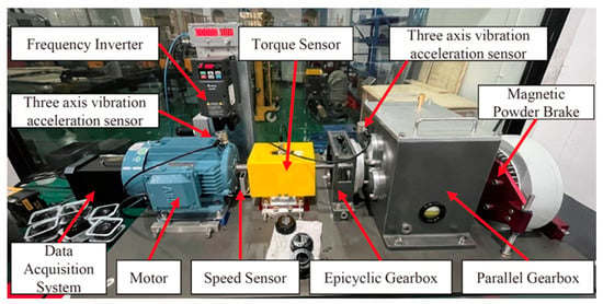
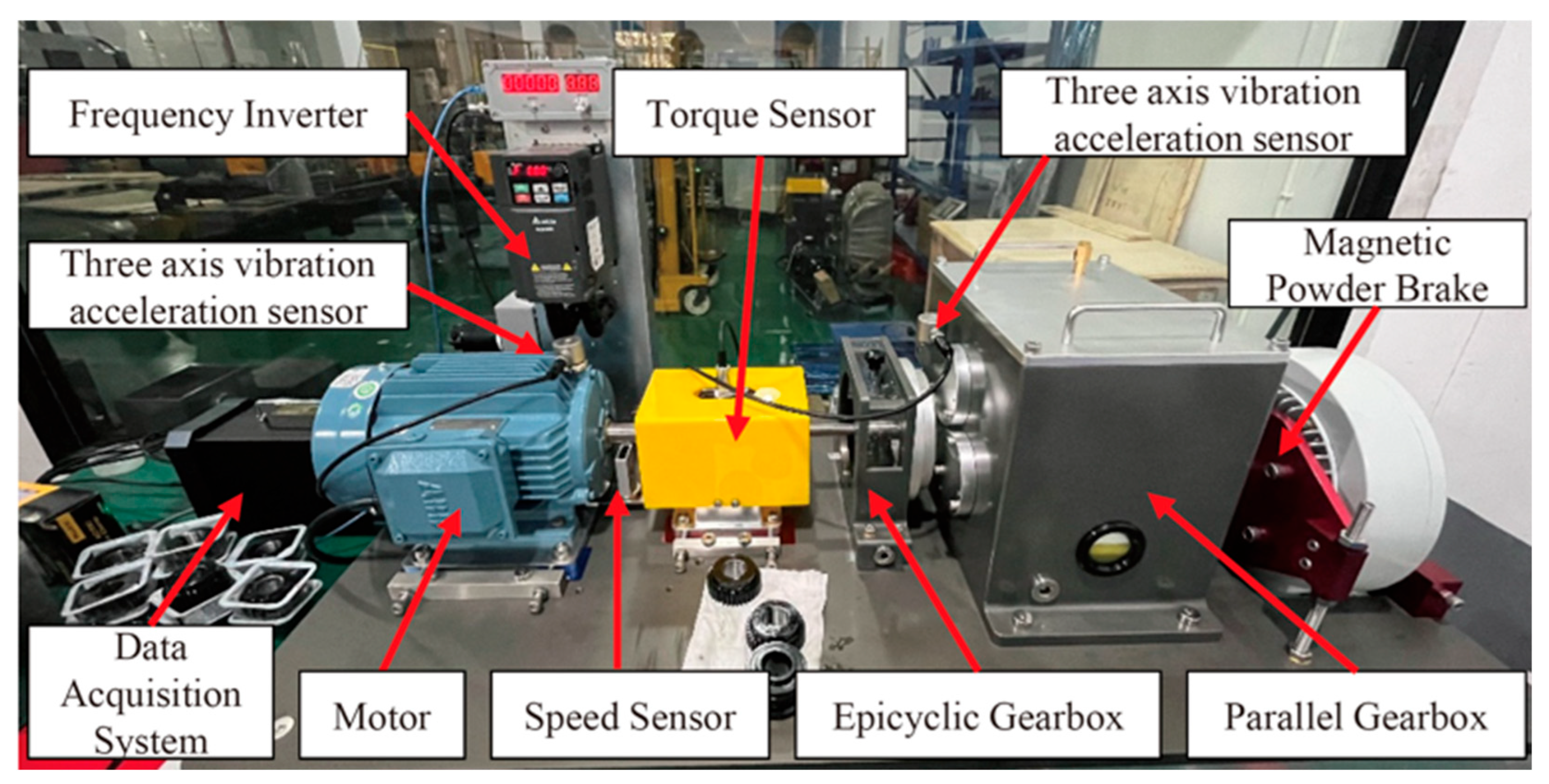
The dataset used in this study is a multimode gearbox fault-diagnosis dataset collected under variable operating conditions. It contains vibration, rotational-speed, and torque signals [29]. As shown in Figure 2, the test rig consists of a motor, a planetary gearbox, a parallel-shaft gearbox, speed and torque sensors, a magnetic-powder brake, and a data-acquisition system. The physical parameters of the test gearbox are listed in Table 2. Unlike many existing datasets, each run includes acceleration, constant-speed, and deceleration stages.

Figure 2. Experimental platform of the MCC5-THU gearbox dataset [29].

Table 2. Physical parameters of the test gearbox.

Parameter	Value	Description
Reference shaft	Input shaft (motor output shaft)	First-order reference for order analysis
Input-gear tooth count z1	29	Driving-gear tooth count, first stage
Large intermediate-gear tooth count z2	95	Driven-gear tooth count, first stage
Target-gear tooth count zf	36	Driving-gear tooth count, second stage
Output-gear tooth count zo	90	Driven-gear tooth count, second stage
Target meshing order om	10.9895	Calculated from Equation (11)
Theoretical sideband spacing os	0.3053	Calculated from Equation (11)
Order-integration half-bandwidth Δo	0.10	Energy integrated over a fixed order neighborhood

Table 2. Physical parameters of the test gearbox.

Parameter	Value	Description
Reference shaft	Input shaft (motor output shaft)	First-order reference for order analysis
Input-gear tooth count z1	29	Driving-gear tooth count, first stage
Large intermediate-gear tooth count z2	95	Driven-gear tooth count, first stage
Target-gear tooth count zf	36	Driving-gear tooth count, second stage
Output-gear tooth count zo	90	Driven-gear tooth count, second stage
Target meshing order om	10.9895	Calculated from Equation (11)
Theoretical sideband spacing os	0.3053	Calculated from Equation (11)
Order-integration half-bandwidth Δo	0.10	Energy integrated over a fixed order neighborhood

The speed channel provides a once-per-revolution phase-reference pulse rather than a directly usable continuous speed measurement. Valid rising edges are detected first, and their sample positions p_k are recorded. Two adjacent edges correspond to one reference-shaft revolution, from which the interval speed is calculated. Each interval speed is assigned to the midpoint between the two pulses, and linear interpolation then gives a speed sequence synchronized sample by sample with the vibration signal. This sequence is used to calculate the mean speed of each window. The pulse time, interval speed, and mean window speed are:

$$\begin{array}{c}{t}_k={\displaystyle \frac{p_k}{f_s}},\\ n_k={\displaystyle \frac{60}{t_{k+1}-t_k}}={\displaystyle \frac{60f_s}{p_{k+1}-p_k}},\\ s_i={\displaystyle \frac{1}{L}}{\displaystyle \sum _{r=0}^{L-1}}{n}_{\left(i-1\right)H+r}.\end{array}$$

(30)

where f_s is the sampling frequency, p_k is the sample index of the kth valid rising edge, t_k is its time, n_k is the reference-shaft speed between two adjacent pulses, n_(i−1)H + r is the interpolated synchronized speed at the rth sample of the ith window, and s_i is the mean window speed. Each s_i is paired with one vibration window and is used for PCC selection and for fitting the healthy speed trends of the statistical and mechanism features.

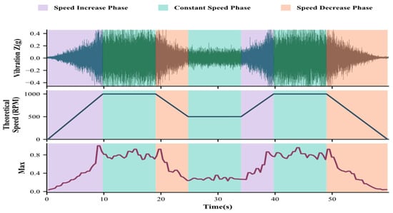
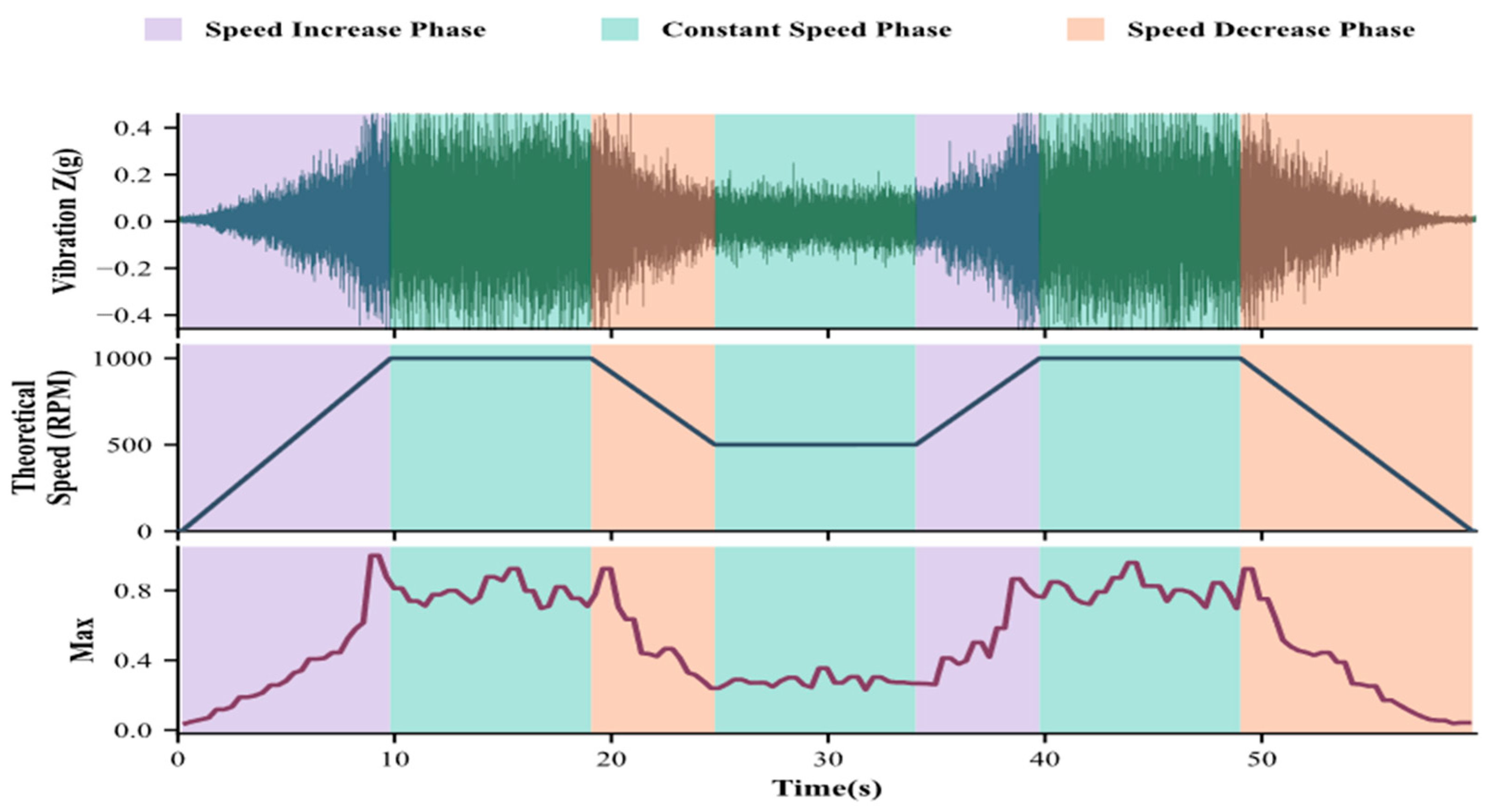
Figure 3 shows that the maximum windowed vibration amplitude changes with the speed stage, confirming that the raw features are nonstationary even in the healthy state. Tests were conducted at 10 and 20 Nm. The four fault types were tooth-surface pitting, a missing tooth, a broken tooth combined with an inner-race bearing fault, and a broken tooth combined with an outer-race bearing fault. The test groups are listed in Table 3.

Figure 3. Visualization of the dataset signals.

Table 3. Experimental groups.

Group	Fault Type	Sampling Frequency	Load	Duration	Speed Range (rpm)
F1	Pitting	12.8 kHz	10/20 Nm	180 s	0–1000
F2	Missing tooth			60 s
F3	Broken tooth + inner-race bearing fault			180 s
F4	Broken tooth + outer-race bearing fault			180 s

The MCC5-THU fault specimens were prepared by laser machining with an accuracy of 0.01 mm [29]. Gear defects were introduced on the 36-tooth gear mounted on the intermediate shaft. Bearing defects were introduced on the ER16K support bearing located at the end of the same shaft, near the faulty gear. Pitting severity was defined by the diameter of a single pit, broken-tooth severity by the fraction of tooth width removed, and bearing-fault severity by the width of the machined defect on the inner or outer raceway.

The tests at 10 Nm included light pitting with a pit diameter of 0.5 mm; one missing-tooth fault; medium and high broken-tooth faults combined with the corresponding inner-race defects; and light, medium, and high broken-tooth faults combined with the corresponding outer-race defects. The tests at 20 Nm included light and high pitting with pit diameters of 0.5 and 1.5 mm, one missing-tooth fault, the same two inner-race compound-fault levels, and the same three outer-race compound-fault levels. For the compound faults, the light, medium, and high broken-tooth levels corresponded to the removal of one quarter, one half, and three quarters of the tooth width, respectively. The corresponding raceway-defect widths were 0.1, 0.3, and 0.5 mm.

3.2. Experimental Setup

Separate models were constructed for the 10 and 20 Nm conditions. For each load condition, the corresponding healthy record was used to fit the statistical and mechanism speed trends, calculate the RB-HCW weights, train DeepSVDD, and set the anomaly threshold. Fault records were used only for evaluation. All fitted trends, weights, model parameters, and thresholds were specific to the corresponding load.

For each load and speed range, the dataset contains one healthy record covering a complete variable-speed cycle with acceleration, constant-speed, and deceleration stages. The record is retained as a whole so that trend fitting covers the available operating range and the chronological sequence required by SBQA is preserved. Because no repeated healthy cycle is available under the same condition, the resulting healthy-state statistics characterize the available record rather than an independent repeat of that cycle.

Within each record, the signal was divided chronologically into 9126-sample candidate windows with a step of 4563 samples, corresponding to 50% overlap. The windows retained their temporal order, and all healthy data were used for training. Statistical features were calculated from these candidates, whereas mechanism features were obtained from the aligned four-revolution segments defined in Section 2.3. Candidates that could not support four complete revolutions were removed, and the same retained indices were used for every method. This procedure retained 162 to 164 of the original 167 candidate windows in each record. The mean speeds of the retained windows ranged from 75.90 to 981.75 rpm, and the aligned four-revolution segments spanned 0.244 to 2.985 s.

The detection threshold for each method is fixed at the 92nd percentile of its own healthy anomaly-score distribution. Table 4 summarizes the remaining implementation settings.All algorithms were implemented in Python 3.12. The deep learning models were implemented using PyTorch 2.9.0, and the baseline models were implemented using scikit-learn 1.7.2.

Table 4. Implementation settings for the anomaly-detection models.

Parameter	Setting	Description
Shared preprocessing	9126 samples, 50% overlap, four-revolution segments, 2048-order samples	Identical retained windows and fused features for all methods
Shared protocol	92nd percentile threshold, random seed 42, SBQA disabled	Common evaluation protocol for Table 5, Table 6 and Table 7
MCD	Automatic support fraction	Squared Mahalanobis distance
IForest	200 trees, contamination = 0.08	Negative decision function
LOF	20 neighbors, novelty mode, contamination = 0.08	Negative decision function
OCSVM	RBF kernel, gamma = scale, nu = 0.08	Negative decision function
VAE	d-64-32-8-32-64-d, KL weight = 0.001	Adam, learning rate 0.001, weight decay 0.000001, 80 epochs, batch size 128, reconstruction error
AE	d-64-32-8-32-64-d	Adam, learning rate 0.001, weight decay 0.000001, 80 epochs, batch size 128, reconstruction error
Proposed	Bias-free d-64-32-8	Adam, learning rate 0.001, weight decay 0.000001, 80 epochs, batch size 128, Euclidean center distance

3.3. Comparison Methods and Evaluation Metrics

The proposed method was compared with six anomaly-detection models. All detectors were evaluated on the same retained windows and received the same fused input, comprising the speed-residual statistical features and the five RB-HCW-weighted mechanism residuals. Because training used healthy data only, supervised classifiers were excluded. The baselines were the minimum covariance determinant (MCD) [30], Isolation Forest (IForest) [31], local outlier factor (LOF) [32], one-class support vector machine (OCSVM) [33], variational autoencoder (VAE) [34], and autoencoder (AE) [35].

Performance was assessed using true positive rate (TPR), accuracy (ACC), and F1-score. TPR is the proportion of fault samples correctly detected, ACC is the overall proportion of correct decisions, and F1-score balances precision and TPR. SBQA was disabled in Table 5, Table 6 and Table 7, so these results compare the window-level detectors before sequence confirmation. Section 3.6 examines the effect of sequence confirmation on the false-positive rate (FPR). The metrics are defined below.

$$\mathrm{TPR}={\displaystyle \frac{\mathrm{TP}}{\mathrm{TP}+\mathrm{FN}}}$$

(31)

$$\mathrm{ACC}={\displaystyle \frac{\mathrm{TP}+\mathrm{TN}}{\mathrm{TP}+\mathrm{TN}+\mathrm{FP}+\mathrm{FN}}}$$

(32)

$$\mathrm{Pr}={\displaystyle \frac{\mathrm{TP}}{\mathrm{TP}+\mathrm{FP}}}$$

(33)

$$\mathrm{F}1-\mathrm{score}={\displaystyle \frac{2\times \mathrm{Pr}\times \mathrm{TPR}}{\mathrm{Pr}+\mathrm{TPR}}}$$

(34)

Table 5. Anomaly-detection performance of the compared methods on the Tsinghua gearbox dataset at 10 Nm.

Indicator	TPR (%)				ACC (%)				F1-Score (%)
Fault ID	F1	F2	F3	F4	F1	F2	F3	F4	F1	F2	F3	F4
MCD	100.00	89.63	80.37	67.35	96.00	90.80	84.22	73.47	96.17	90.74	87.19	79.23
IForest	92.64	89.02	84.97	62.65	92.31	90.49	87.30	69.94	92.35	90.40	89.94	75.80
LOF	90.18	92.07	76.38	61.02	91.08	92.02	81.56	68.71	91.02	92.07	84.69	74.56
OCSVM	91.41	90.85	83.74	67.76	91.69	91.41	86.48	73.77	91.69	91.41	89.22	79.52
VAE	90.80	94.51	79.14	67.96	91.38	93.25	83.40	73.93	91.36	93.37	86.43	79.67
AE	89.57	94.51	79.75	68.16	90.77	93.25	83.81	74.08	90.68	93.37	86.81	79.81
Proposed	96.93	96.95	88.96	88.16	94.46	94.48	89.96	89.11	94.61	94.64	92.21	92.41

Table 6. Anomaly-detection performance of the compared methods on the Tsinghua gearbox dataset at 20 Nm.

Indicator	TPR (%)				ACC (%)				F1-Score (%)
Fault ID	F1	F2	F3	F4	F1	F2	F3	F4	F1	F2	F3	F4
MCD	92.64	87.12	84.97	80.82	92.43	89.57	87.32	83.61	94.23	89.31	89.94	88.10
IForest	95.09	46.01	83.74	76.53	94.07	69.02	86.50	80.40	95.53	59.76	89.22	85.42
LOF	81.60	86.50	77.30	69.39	85.07	89.26	82.21	75.04	87.93	88.96	85.28	80.66
OCSVM	94.79	95.71	85.89	88.78	93.87	93.87	87.93	89.59	95.37	93.98	90.47	92.75
VAE	88.04	93.87	75.77	72.04	89.37	92.94	81.19	77.03	91.69	93.01	84.30	82.48
AE	91.72	93.87	79.14	79.18	91.82	92.94	83.44	82.39	93.73	93.01	86.43	87.09
Proposed	96.32	95.09	90.80	93.27	94.89	93.56	91.21	92.96	96.17	93.66	93.23	95.21

Table 7. Mean results over the two load conditions.

Method	TPR (%)	ACC (%)	F1-Score (%)
MCD	85.36	87.18	89.36
IForest	78.83	83.75	84.80
LOF	79.31	83.12	85.65
OCSVM	87.36	88.58	90.55
VAE	82.76	85.31	87.79
AE	84.49	86.56	88.87
Proposed	93.31	92.58	94.02

Here, true positives (TP) and true negatives (TN) denote the numbers of fault and healthy samples classified correctly, respectively. False positives (FP) denote the number of healthy samples incorrectly classified as faulty, and false negatives (FN) denote the number of fault samples incorrectly classified as healthy. Pr denotes precision.

3.4. Comparison Results and Discussion

Table 5 and Table 6 report the detector performance at 10 and 20 Nm using fixed four-revolution segments. All methods are evaluated on the same retained samples and fused features, with SBQA disabled. Table 7 gives the macro-average over the two loads and four fault types, calculated from the unrounded fault-level results before rounding to two decimal places.

The proposed method ranked first in 18 of the 24 fault-specific metric entries and achieved the highest macro-average for each metric. At 10 Nm, MCD achieved the highest scores for fault F1, whereas the proposed method achieved the highest TPR, ACC, and F1-score values for faults F2 through F4. At 20 Nm, OCSVM achieved the highest scores for fault F2, whereas the proposed method led all three metrics for faults F1, F3, and F4. Across all load and fault combinations, the proposed method achieved macro-averaged TPR, ACC, and F1-score values of 93.31%, 92.58%, and 94.02%. These values exceeded the corresponding second-best averages by 5.95, 4.00, and 3.47 percentage points. Although no detector led for every fault type, the proposed method achieved the highest overall averages.

3.5. Ablation Study

Ablation tests at 10 and 20 Nm and across fault types F1–F4 were used to isolate the contribution of each module. Three model configurations were compared:

M1: DeepSVDD using statistical features derived from the speed residuals. M1 serves as the baseline model;

M2: M1 augmented with five mechanism-based residual features;

M3: M2 with RB-HCW weighting applied to the five mechanism-based residual features.

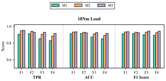
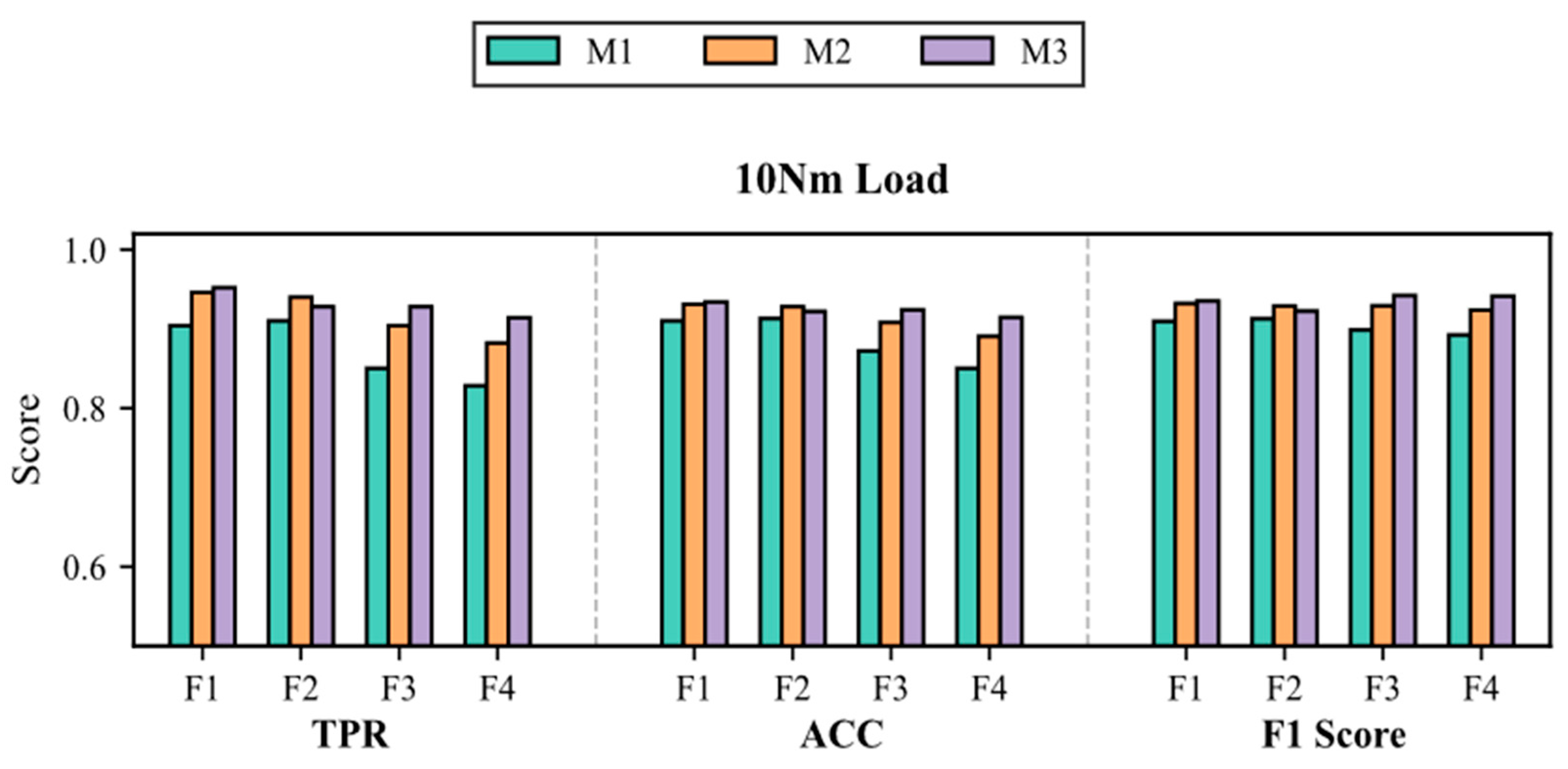
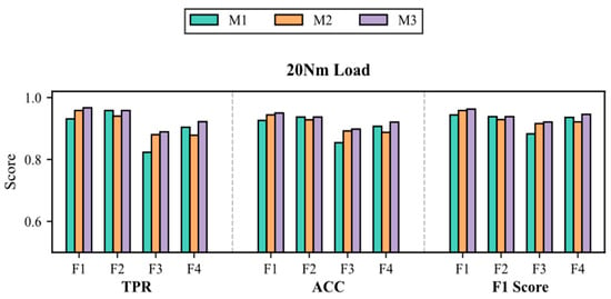
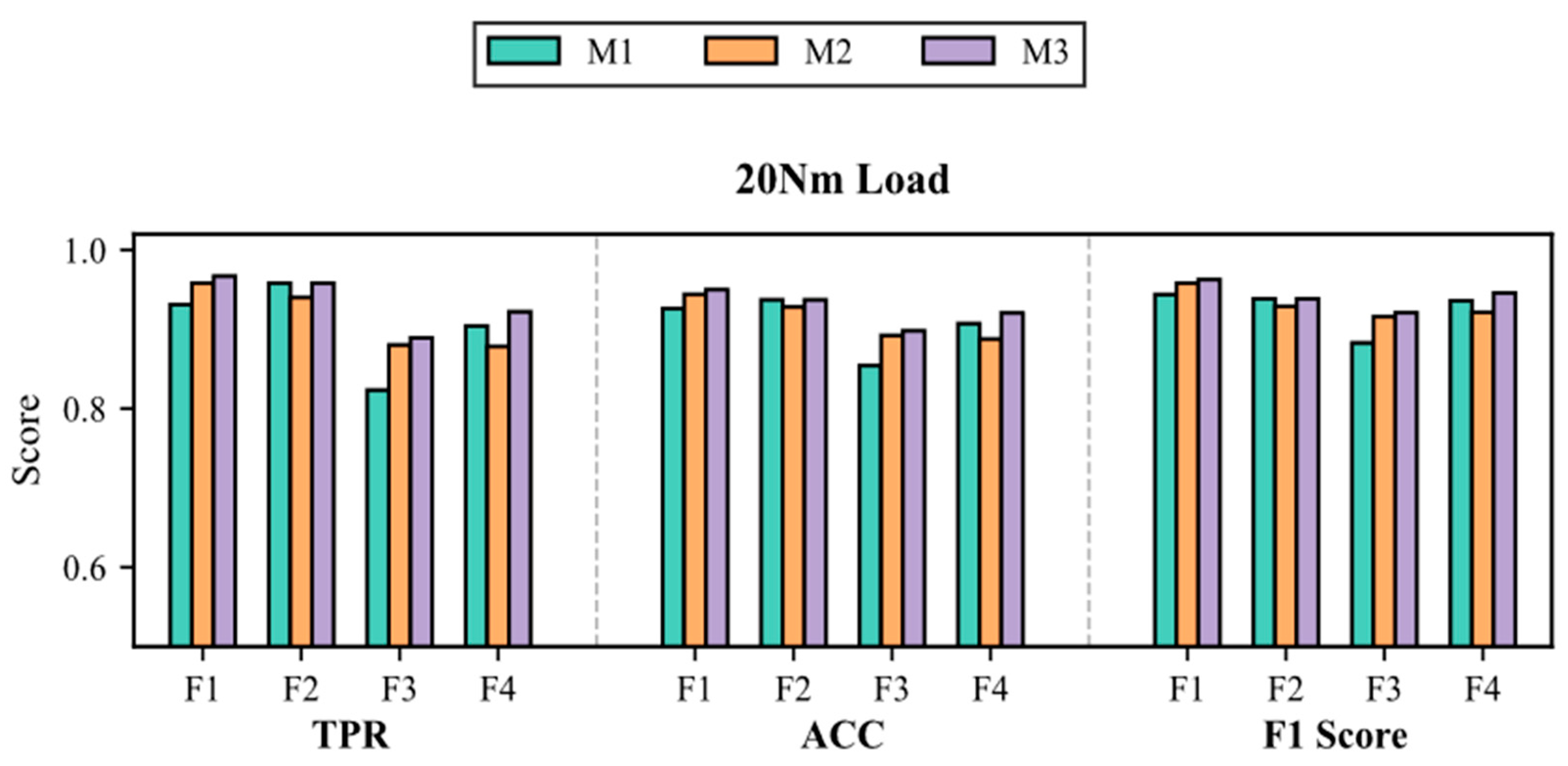
Figure 4 and Figure 5 show the fault-specific changes across M1, M2, and M3. Adding the five mechanism residuals in M2 mainly improves F3 and F4 at 10 Nm and F1 and F3 at 20 Nm. Applying RB-HCW in M3 reduces variation across loads and fault types, particularly for the compound faults. The mechanism branch supplies meshing, harmonic, and modulation information that is not fully captured by the speed-residual statistics, while RB-HCW reduces the influence of mechanism residuals that are unstable in healthy data.

Figure 4. Ablation results on the Tsinghua gearbox dataset under the 10 Nm load.

Figure 5. Ablation results on the Tsinghua gearbox dataset under the 20 Nm load.

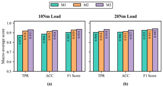
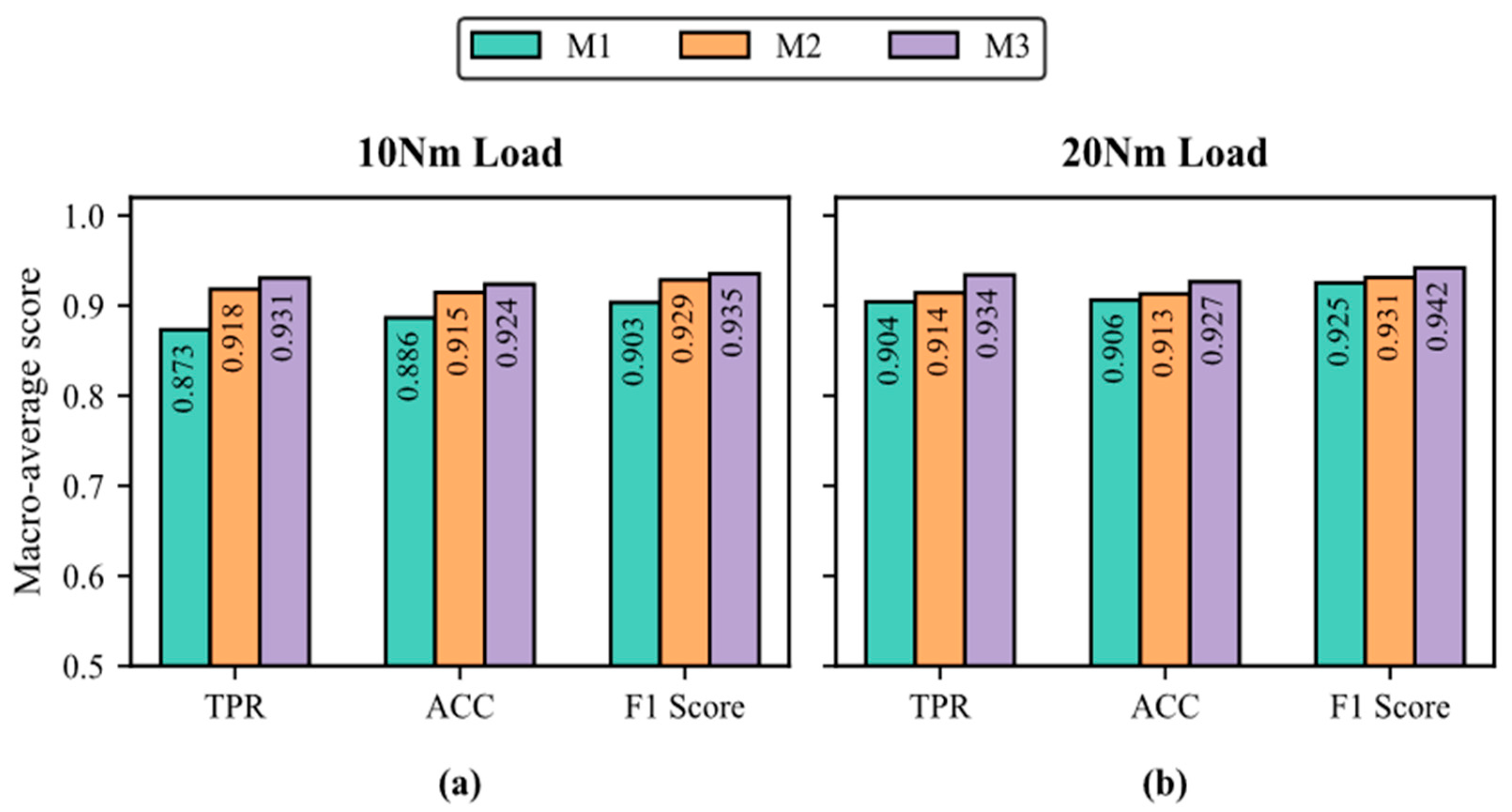
Figure 6 summarizes the average changes across fault types. Relative to M1, M2 increases the two-load average TPR, ACC, and F1-score by 2.75, 1.80, and 1.60 percentage points, respectively. Adding RB-HCW raises M3 above M2 by a further 1.65, 1.15, and 0.85 percentage points. Overall, M3 exceeds M1 by 4.40, 2.95, and 2.45 percentage points for the same metrics. Because M2 adds all five mechanism residuals simultaneously, this comparison measures their joint contribution rather than the effect of an individual indicator.

Figure 6. Mean ablation results: (a) 10 Nm and (b) 20 Nm.

Figure 6 shows the combined contribution of the five mechanism indicators, but it does not reveal the specific role of each indicator. We therefore compared the statistical-residual baseline with five single-indicator configurations and the complete feature set. The indicators h1 to h5 are defined in Section 2.3, and DeepSVDD was retrained for each configuration. RB-HCW and SBQA were disabled to prevent consistency weighting and alarm confirmation from influencing the comparison. Under this setting, performance differences among the configurations mainly reflect changes in feature composition. Table 8 and Table 9 present the results for 10 and 20 Nm, respectively.

Table 8. Incremental contribution of individual mechanism features at 10 Nm.

Configuration	TPR (%)	ACC (%)	F1-Score (%)
Stat. only	89.07	89.61	91.31
Stat. + h1	86.23	87.95	89.70
Stat. + h2	87.72	89.00	90.59
Stat. + h3	88.62	89.40	91.07
Stat. + h4	89.40	89.93	91.51
Stat. + h5	87.92	89.01	90.68
Stat. + h1–h5	93.81	92.79	93.93

Table 9. Incremental contribution of individual mechanism features at 20 Nm.

Configuration	TPR (%)	ACC (%)	F1-Score (%)
Stat. only	84.26	86.64	88.99
Stat. + h1	86.88	88.21	90.46
Stat. + h2	86.23	87.82	90.13
Stat. + h3	86.95	88.35	90.54
Stat. + h4	89.35	89.73	91.91
Stat. + h5	91.17	91.18	92.97
Stat. + h1–h5	94.91	93.82	95.01

The contribution of individual mechanism indicators varied with load. At 10 Nm, h4 was the only indicator to improve TPR, ACC, and F1-score simultaneously over the statistical-residual baseline. In contrast, all five indicators improved the three metrics at 20 Nm, with h5 producing the largest gains and h4 the next largest. Despite this load dependence, the complete feature set outperformed every single-indicator configuration under both loads. For the complete set, TPR, ACC, and F1-score reached 93.81%, 92.79%, and 93.93% at 10 Nm and 94.91%, 93.82%, and 95.01% at 20 Nm. The consistent advantage of the complete set shows that the indicators differ in their load-specific contributions but provide complementary information when used together.

The contribution of each indicator within the complete group was also tested by removing one feature at a time. Table 10 and Table 11 report the leave-one-feature-out results.

Table 10. Leave-one-feature-out results for the mechanism feature set at 10 Nm.

Configuration	TPR (%)	ACC (%)	F1-Score (%)
h1–h5	93.81	92.79	93.93
Without h1	93.04	92.33	93.52
Without h2	92.39	91.94	93.18
Without h3	92.76	92.20	93.38
Without h4	90.52	90.61	92.13
Without h5	91.19	91.30	92.53

Table 11. Leave-one-feature-out results for the mechanism feature set at 20 Nm.

Configuration	TPR (%)	ACC (%)	F1-Score (%)
h1–h5	94.91	93.82	95.01
Without h1	91.27	91.14	93.01
Without h2	88.30	89.20	91.37
Without h3	88.35	89.21	91.39
Without h4	91.92	91.82	93.40
Without h5	88.77	89.45	91.59

The leave-one-feature-out results clarify how the five indicators complement one another. At 10 Nm, removing h4 caused the largest decrease across all three metrics, followed by h5. At 20 Nm, the largest losses occurred after removing h2, h3, or h5. The results for h2 and h3 are particularly informative. Their standalone gains at 20 Nm were smaller than those of h4 and h5, yet removing either feature from the complete set caused one of the largest performance losses. Their contributions are, therefore, more apparent within the combined representation than when either feature is used alone. None of the tested reduced configurations matched the complete set under either load, so all five indicators were retained. Because M2 and M3 in Figure 6 use the same five-indicator set, the improvement from M2 to M3 reflects the effect of RB-HCW rather than a change in feature composition.

3.6. Sensitivity Analysis of the Alarm Parameters

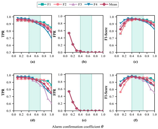
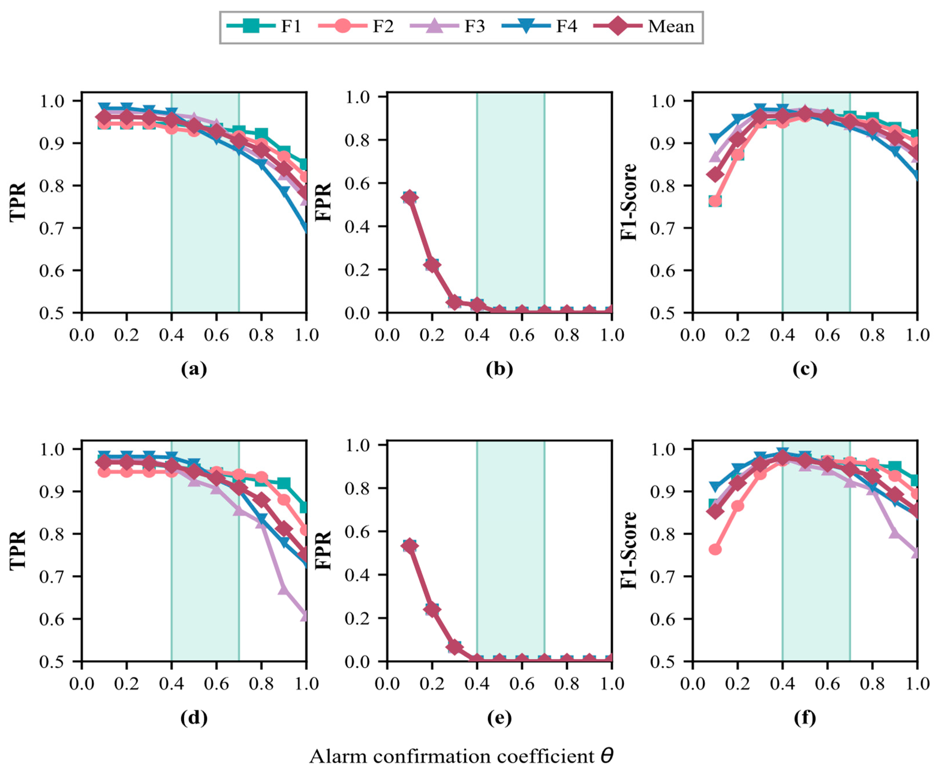
The queue length was fixed at 10, and θ was varied from 0.1 to 1.0 to examine its effect on SBQA.

As shown in Figure 7, when θ is between 0.1 and 0.3, only a few anomalous windows are needed to issue an alarm. TPR remains high for every fault, but occasional threshold crossings in healthy data are also confirmed readily, producing a high FPR and limiting the F1-score. As θ increases to 0.4–0.7, FPR falls rapidly toward zero while TPR remains high for most faults, and the F1-score enters a stable range. FPR in this analysis is calculated from the final SBQA alarm sequence rather than from the initial window-level threshold crossings. At larger θ values, the stricter confirmation rule keeps the FPR low but increases missed detections and confirmation delay.

Figure 7. Effect of the alarm-confirmation coefficient θ on anomaly-detection performance: (a–c) 10 Nm and (d–f) 20 Nm on the Tsinghua gearbox dataset. The green shaded region indicates the recommended range of θ identified in this study.

The two load conditions showed similar trends, although sensitivity to θ differed by fault type. The TPR for faults F3 and F4 declined more noticeably at higher θ values, indicating that the compound faults were more sensitive to a strict confirmation criterion. Considering TPR, FPR, and F1-score together, values from 0.4 to 0.7 provide a practical range. This study used θ = 0.7, which requires at least 7 anomalous decisions among the 10 most recent windows before an alarm is issued. This setting maintained a high TPR while strongly suppressing false alarms. It is not universally optimal and should be adjusted according to the sampling interval, allowable alarm delay, persistence of the fault response, and cost of false alarms.

4. Conclusions

Speed-dependent drift reduces the separation between healthy and faulty gearbox vibration features. The proposed framework models residuals from healthy speed trends in parallel statistical and order-domain branches to counter this drift. The statistical branch captures broad changes in the vibration signal, while the mechanism branch models meshing energy, harmonic structure, sideband modulation, and order-spectrum complexity. Before fusion, RB-HCW reduces the influence of unstable mechanism residuals, and DeepSVDD learns the healthy distribution of the combined representation. SBQA then checks whether abnormal decisions persist across successive windows before it issues an alarm.

Across four fault types under two independently modeled load conditions, the proposed method achieved macro-averaged TPR, ACC, and F1-score values of 93.31%, 92.58%, and 94.02%. It ranked first in most fault-specific comparisons and achieved the highest overall average for all three metrics.

The ablation study isolates the effects of the mechanism residuals and RB-HCW. At 10 Nm, M3 improves TPR, ACC, and F1-score over M1 by 6.64%, 4.29%, and 3.54% in relative terms, corresponding to increases of 5.80, 3.80, and 3.20 percentage points. At 20 Nm, the relative improvements are 3.32%, 2.32%, and 1.84%, corresponding to increases of 3.00, 2.10, and 1.70 percentage points. The results indicate that the mechanism residuals supplement the statistical branch and that RB-HCW stabilizes their contribution.

SBQA was introduced to prevent an isolated threshold crossing from triggering an alarm. It updates a Beta posterior from decisions over consecutive windows and issues an alarm only after the confirmation condition is met. The sensitivity study, conducted with a queue length of 10, showed that the confirmation coefficient affects the detection sensitivity, false-alarm rate, and delay simultaneously. The coefficient should, therefore, be chosen with reference to the sampling interval, allowable delay, and false-alarm cost. Compared with single-window decisions, SBQA reduces the alarms caused by isolated abnormal points and gives more stable results in continuous monitoring.

These results support the use of the proposed framework for load-specific anomaly detection under variable-speed conditions, but they do not establish transferability across load conditions. Healthy-state and fault-state data are stored in separate records, and the fault-onset time is not documented. The physical fault-to-alarm delay, therefore, cannot be measured directly. Future work will evaluate the framework using repeated healthy cycles and independent records containing previously unseen speed ranges. Continuous records with known fault-onset times will also be used to quantify alarm delay and examine how the SBQA settings balance response time against false-alarm suppression.

References

- Ye, J.; Wei, J.; Zhang, A.; Chen, S.; Ran, T.; Shu, R. Theoretical and experimental study on the dynamic behavior of spur gear transmission system during hovering maneuver flights. Mech. Syst. Signal Process. 2024, 212, 111296. [Google Scholar] [CrossRef] [Scilit]
- Dubaish, A.A.; Jaber, A.A. State-of-the-art review into signal processing and artificial intelligence-based approaches applied in gearbox defect diagnosis. Eng. Technol. J. 2024, 42, 157–172. [Google Scholar] [CrossRef] [Scilit]
- Lei, Y.; Lin, J.; Zuo, M.J.; He, Z. Condition monitoring and fault diagnosis of planetary gearboxes: A review. Measurement 2014, 48, 292–305. [Google Scholar] [CrossRef] [Scilit]
- Liu, D.; Cui, L.; Cheng, W. A review on deep learning in planetary gearbox health state recognition: Methods, applications, and dataset publication. Meas. Sci. Technol. 2024, 35, 012002. [Google Scholar] [CrossRef] [Scilit]
- Feng, X.; Zhang, T. A hierarchical attention-guided data–knowledge fusion network for few-shot gearboxes’ fault diagnosis. Machines 2025, 13, 486. [Google Scholar] [CrossRef] [Scilit]
- Wang, B.; Zhao, S. MTAGCN: Multi-task graph-guided convolutional network with attention mechanism for intelligent fault diagnosis of rotating machinery. Machines 2025, 13, 347. [Google Scholar] [CrossRef] [Scilit]
- Chai, S.; Xu, K. Instantaneous frequency analysis based on high-order multisynchrosqueezing transform on motor current and application to RV gearbox fault diagnosis. Machines 2025, 13, 223. [Google Scholar] [CrossRef] [Scilit]
- Seo, M.-K.; Yun, W.-Y. Gearbox condition monitoring and diagnosis of unlabeled vibration signals using a supervised learning classifier. Machines 2024, 12, 127. [Google Scholar] [CrossRef] [Scilit]
- Kumar, R.; Kumar, P.; Vashishtha, G.; Chauhan, S.; Zimroz, R.; Kumar, S.; Kumar, R.; Gupta, M.K.; Ross, N.S. Fault identification of direct-shift gearbox using variational mode decomposition and convolutional neural network. Machines 2024, 12, 428. [Google Scholar] [CrossRef] [Scilit]
- Randall, R.B. Vibration-based diagnostics of gearboxes under variable speed and load conditions. Meccanica 2016, 51, 3227–3239. [Google Scholar] [CrossRef] [Scilit]
- Urbanek, J.; Barszcz, T.; Antoni, J. A two-step procedure for estimation of instantaneous rotational speed with large fluctuations. Mech. Syst. Signal Process. 2013, 38, 96–102. [Google Scholar] [CrossRef] [Scilit]
- Fyfe, K.R.; Munck, E.D.S. Analysis of computed order tracking. Mech. Syst. Signal Process. 1997, 11, 187–205. [Google Scholar] [CrossRef] [Scilit]
- Song, H.; Sun, Y.; Gao, H.; You, Z.; Xu, H. Residual feature-based semi-supervised anomaly detection for gearbox under varying rotational speeds. Measurement 2025, 256, 118236. [Google Scholar] [CrossRef] [Scilit]
- Li, J.; Liu, S.; Li, S.; Wang, Y.; Cheng, Z.; Wu, Y. A mechanism-informed contrastive learning framework for zero-shot gear anomaly detection. Measurement 2026, 257, 118905. [Google Scholar] [CrossRef] [Scilit]
- Zhao, X.; Yao, J.; Deng, W.; Ding, P.; Ding, Y.; Jia, M.; Liu, Z. Intelligent fault diagnosis of gearbox under variable working conditions with adaptive intraclass and interclass convolutional neural network. IEEE Trans. Neural Netw. Learn. Syst. 2023, 34, 6339–6353. [Google Scholar] [CrossRef] [Scilit] [PubMed]
- Hu, C.; Wu, J.; Sun, C.; Chen, X.; Yan, R. Mutual information-based feature disentangled network for anomaly detection under variable working conditions. Mech. Syst. Signal Process. 2023, 204, 110804. [Google Scholar] [CrossRef] [Scilit]
- Zhou, H.; Huang, X.; Wen, G.; Dong, S.; Lei, Z.; Zhang, P.; Chen, X. Convolution enabled transformer via random contrastive regularization for rotating machinery diagnosis under time-varying working conditions. Mech. Syst. Signal Process. 2022, 173, 109050. [Google Scholar] [CrossRef] [Scilit]
- Xu, Q.; Xie, T.; Jiang, C.; Cheng, Q.; Wang, X. Adaptive working condition recognition with clustering-based contrastive learning for unsupervised anomaly detection. IEEE Trans. Ind. Inf. 2024, 20, 12103–12113. [Google Scholar] [CrossRef] [Scilit]
- Li, Q.; Shen, C.; Chen, L.; Zhu, Z. Knowledge mapping-based adversarial domain adaptation: A novel fault diagnosis method with high generalizability under variable working conditions. Mech. Syst. Signal Process. 2021, 147, 107095. [Google Scholar] [CrossRef] [Scilit]
- Li, G.; Wei, M.; Wu, D.; Cheng, Y.; Wu, J.; Yan, J. Zero-sample fault diagnosis of rolling bearings via fault spectrum knowledge and autonomous contrastive learning. Expert Syst. Appl. 2025, 275, 127080. [Google Scholar] [CrossRef] [Scilit]
- Hendrickx, K.; Meert, W.; Mollet, Y.; Gyselinck, J.; Cornelis, B.; Gryllias, K.; Davis, J. A general anomaly detection framework for fleet-based condition monitoring of machines. Mech. Syst. Signal Process. 2020, 139, 106585. [Google Scholar] [CrossRef] [Scilit]
- Pang, G.; Shen, C.; Cao, L.; van den Hengel, A. Deep learning for anomaly detection: A review. ACM Comput. Surv. 2022, 54, 1–38. [Google Scholar] [CrossRef] [Scilit]
- Tax, D.M.J.; Duin, R.P.W. Support vector data description. Mach. Learn. 2004, 54, 45–66. [Google Scholar] [CrossRef] [Scilit]
- Ruff, L.; Vandermeulen, R.; Görnitz, N.; Deecke, L.; Siddiqui, S.A.; Binder, A.; Müller, E.; Kloft, M. Deep one-class classification. In Proceedings of the 35th International Conference on Machine Learning; PMLR: Cambridge, MA, USA, 2018; Volume 80, pp. 4393–4402. [Google Scholar]
- Peng, D.; Desmet, W.; Gryllias, K. Reconstruction-based deep unsupervised adaptive threshold support vector data description for wind turbine anomaly detection. Reliab. Eng. Syst. Saf. 2025, 260, 110995. [Google Scholar] [CrossRef] [Scilit]
- Barandas, M.; Folgado, D.; Fernandes, L.; Santos, S.; Abreu, M.; Bota, P.; Liu, H.; Schultz, T.; Gamboa, H. TSFEL: Time series feature extraction library. SoftwareX 2020, 11, 100456. [Google Scholar] [CrossRef] [Scilit]
- Edelmann, D.; Mori, T.F.; Székely, G.J. On relationships between the Pearson and the distance correlation coefficients. Stat. Probab. Lett. 2021, 169, 108960. [Google Scholar] [CrossRef] [Scilit]
- Gao, P.; Yan, Q.; Liu, H.; Xiang, C.; Chen, K. Research on fault characteristics and signal transfer path mechanism of the gear transmission system. Mech. Syst. Signal Process. 2025, 228, 112471. [Google Scholar] [CrossRef] [Scilit]
- Chen, S.; Liu, Z.; He, X.; Zou, D.; Zhou, D. Multi-mode fault diagnosis datasets of gearbox under variable working conditions. Data Brief 2024, 54, 110453. [Google Scholar] [CrossRef] [Scilit] [PubMed]
- Rousseeuw, P.J.; Van Driessen, K. A fast algorithm for the minimum covariance determinant estimator. Technometrics 1999, 41, 212–223. [Google Scholar] [CrossRef]
- Puggini, L.; McLoone, S. An enhanced variable selection and Isolation Forest based methodology for anomaly detection with OES data. Eng. Appl. Artif. Intell. 2018, 67, 126–135. [Google Scholar] [CrossRef] [Scilit]
- Breunig, M.M.; Kriegel, H.-P.; Ng, R.T.; Sander, J. LOF: Identifying density-based local outliers. In Proceedings of the 2000 ACM SIGMOD International Conference on Management of Data, Dallas, TX, USA, 16–18 May 2000; pp. 93–104. [Google Scholar] [CrossRef] [Scilit]
- Fernández-Francos, D.; Martínez-Rego, D.; Fontenla-Romero, O.; Alonso-Betanzos, A. Automatic bearing fault diagnosis based on one-class ν-SVM. Comput. Ind. Eng. 2013, 64, 357–365. [Google Scholar] [CrossRef] [Scilit]
- Yokkampon, U.; Chumkamon, S.; Mowshowitz, A.; Hayashi, E. Anomaly detection using variational autoencoder with spectrum analysis for time series data. In Proceedings of the 2020 Joint 9th International Conference on Informatics, Electronics & Vision and 4th International Conference on Imaging, Vision & Pattern Recognition; IEEE: Piscataway, NJ, USA, 2020; pp. 1–6. [Google Scholar]
- Huang, W.; Zhang, B.; Zhang, K.; Gao, H.; Wan, R. Improved autoencoder with LSTM module and KL divergence for anomaly detection. IEEE Trans. Instrum. Meas. 2024, 73, 3534011. [Google Scholar] [CrossRef] [Scilit]
Disclaimer/Publisher’s Note: The statements, opinions and data contained in all publications are solely those of the individual author(s) and contributor(s) and not of MDPI and/or the editor(s). MDPI and/or the editor(s) disclaim responsibility for any injury to people or property resulting from any ideas, methods, instructions or products referred to in the content. |
© 2026 by the authors. Licensee MDPI, Basel, Switzerland. This article is an open access article distributed under the terms and conditions of the Creative Commons Attribution (CC BY) license.