Open-End Winding Induction Machine Drives Under Unbalanced Phase Impedances

Abstract

Manufacturing tolerances and winding-layout variations can introduce phase-to-phase mismatches in stator resistance and leakage inductance. Under such unbalanced phase impedances, conventional field-oriented control (FOC), typically designed under balanced-parameter assumptions, may produce unequal phase currents, distorted airgap MMF, reduced efficiency, increased torque ripple, and undesired vibro-acoustic behavior. This paper investigates an open-end winding (OEW) induction machine (IM) drive, in which each phase is independently driven by an H-bridge inverter fed by the same DC source. To mitigate phase–current imbalance without parameter estimation, an RMS-based phase–current-balancing controller is proposed. The controller continuously calculates the RMS value of each phase current and adaptively scales the corresponding reference-phase voltage in a low-bandwidth outer loop, while preserving the classical FOC structure. The balancing law is derived directly from the phase-impedance imbalance model; convergence of the three coupled per-phase loops is proven via a Lyapunov argument, and stability of the cascaded structure is established through an analytical bandwidth-separation analysis shown to be robust to ±30% machine-parameter variation and across the 500–1500 rev/min speed range. Simulation and experimental results across multiple operating points demonstrate effective phase–current equalization.

1. Introduction

Electric drives for transportation, industrial automation, and renewable-energy systems are increasingly expected to combine high power density, a wide constant-power speed range, low acoustic noise, and robust operation while meeting efficiency targets. In practice, meeting these goals also requires tolerance to manufacturing and assembly variations that introduce deviations in phase electrical parameters.

Manufacturing tolerances and winding-layout variations can introduce phase-to-phase-impedance imbalance in electric machines, even when the phase windings have the same number of turns by design. For example, differences in the machining and insertion patterns of the slot openings, routing and length of end windings, and even joints, soldering quality, and connection leads can introduce measurable mismatches in phase resistance and leakage inductance [1,2]. The resulting impedance mismatches violate the balanced-parameter assumption that underpins standard three-phase drive models and control design, even in high-performance applications where current quality is tightly regulated [2,3]. Under field-oriented control (FOC), these unequal phase impedances can convert a common-voltage command set into unequal phase–current dynamics, resulting in current imbalance and a distorted airgap magneto motive force (MMF) [3,4]. Consequently, torque ripple, vibration, acoustic noise, and uneven copper loss and uneven thermal loading may increase, reducing both efficiency and drive quality [4,5].

The root of the problem lies in the actuation structure of a conventional three-phase inverter-fed FOC implementation: the controller computes a single-voltage vector, establishing a set of coupled voltage commands for the three phases. When the phase impedances are unequal, the same voltage command does not produce the same current response in each phase, which leads to persistent current imbalance and increased negative-sequence content. This imbalance distorts the airgap MMF and introduces additional spatial and temporal harmonics, resulting in torque ripple and potentially exciting structural resonances, ultimately increasing vibration and acoustic noise [3,4].

Existing mitigation approaches can be grouped into three main families. The first family compensates for the imbalance in the closed loop at the control level: the forward and backward (sequence) current components are extracted, and the backward component is regulated to zero via an additional voltage command within a vector-control framework, thereby improving current symmetry and reducing torque ripple under unbalanced conditions [3,4]. These methods respond within a few fundamental cycles, but they require accurate sequence extraction at the operating frequency, add filters and regulators at the fast control rate, and, more importantly, actuate through the single-voltage vector of a three-leg inverter, which couples the correction applied to one phase to the others. The second family relies on parameter estimation: per-phase parameters, most notably stator-resistance unbalance, are identified online for detection and diagnosis, and a correction can then be applied via the machine model [1,2]. The achievable accuracy of such schemes is, however, tied to excitation richness, measurement noise, and operating-point drift that affect the estimates [1,2]. The impact of residual imbalance on losses, thermal stress, and the resulting operating limits has motivated derating recommendations rather than active correction [5]. The third family acts at the hardware level: external circuits connected in series compensate for the asymmetric phase impedances, suppressing unbalanced currents and the associated torque oscillations [6]. This confirms that impedance balancing at the actuation level is an effective mitigation strategy, but the compensation is fixed by the external elements, cannot track thermal drift, and adds cost and volume. Across all three families, the common limitation is either the shared voltage vector of a single inverter or reliance on an explicit machine model or additional hardware.

Open-end winding (OEW) drive concepts offer an effective architectural remedy because both terminals of each stator phase are accessible, introducing extra degrees of freedom in phase voltage synthesis compared to conventional drives [7,8]. This enables a flexible actuation, with phase voltages shaped and improved control over zero-sequence and common-mode components achieved through suitable modulation in dual-inverter OEW configurations [9,10]. In addition, the OEW concept allows a modular, fault-tolerant machine drive, as, for example, the reconfigurability of phase terminals enables continued operation under open-switch and open-phase faults [11,12]. OEW machine configurations thus continue to attract interest as an enabling platform for novel advanced drive architectures [7,8].

A major stream of OEW research has focused on dual-inverter OEW drives and modulation strategies, including practical OEW implementations for induction machine (IM) drives [7,13]. In dual-inverter OEW drive topologies with independent DC sources, several space–vector modulation (SVM) frameworks have also been proposed to improve voltage utilization and operational flexibility [10]. Such works again highlight the critical importance of modulation–structural design in determining the resulting voltage vector set and associated zero-sequence behavior [14]. For the particular case of OEW drives, specific modulation methods that ensure or regulate zero-sequence voltage components over wide speed ranges have been proposed, as have space–vector pulse-width modulation (SVPWM)-oriented concepts, thus demonstrating the importance of the direct impact of OEW-specific modulation on realistic performance [14,15]. Another important aspect of OEW drives is the issue of current control regulation and the particular form of switching strategy of the associated inverter units, since any improvement in more degrees of freedom at the OEW drive level can only be translated to the actual level if the problems on the inverter side are solved correctly, such as switching actions [16,17].

Beyond modulation design, OEW has also been investigated from a broader system perspective, where additional terminal accessibility can be exploited to improve drive performance under practical non-idealities and operational constraints. In particular, the extra degrees of freedom offered by OEW motivate reliability-oriented operation and control strategies, especially when the drive must sustain acceptable performance under degraded conditions or non-ideal phase behavior [11]. In this sense, one of the other main directions in OEW concerns reliability and fault tolerance, where additional reconfiguration possibilities provide greater freedom. In this respect, some works have investigated isolated DC-bus OEW motor drives under open-switch failure, demonstrating acceptable operation after device faults [11,12]. Integrated post-fault reconfiguration control without topology changes to avoid distortion current and keep operation after a fault within the bounded limits of previously achieved drive performance was proposed in [18,19]. Further studies, for example, support the use of zero-sequence current injection for specific open-circuit faults, confirming the flexibility and attractiveness of the OEW machine system concept for fault handling [20].

Other fundamental works in this area have focused on clarifying the sources of, e.g., the infamous common and circulating currents, and possible strategies to cope with these phenomena arising in practically realized OEW drives. Foundational analyses have identified circulating-current mechanisms in pulse-width modulation (PWM) OEW AC-machine drives and have discussed how these currents can degrade efficiency and increase thermal loading if not properly managed [21,22]. Optimized PWM strategies to reduce common-mode currents in OEW multiphase drives have also been reported, reinforcing that OEW performance depends strongly on how zero-sequence and common-mode quantities are shaped in the inverter [21,23]. This aspect has inspired several multiplication approaches, modulation schemes, and variant-control schemes for OEW topologies, aiming to improve current quality and eliminate circulating-current paths.

Beyond topology and fault tolerance, the OEW concept has found application-oriented motivation for new solutions related to charging integration and electrified powertrains. For instance, several approaches to integrated battery charging based on OEW machines were proposed in the context of an EV-oriented machine concept, enabling charging integration thanks to the accessibility of the windings [24]. In addition, the OEW system of the machine was considered in the concept of wind energy converter systems (WECS) with an integrated converter and machine, thereby further promoting the applicability of OEW to a wide range of energy conversion devices [25]. Furthermore, e-powertrain concepts integrating OEW and winding changeover mechanisms have been proposed to improve efficiency across operating conditions [26,27].

Despite these advances, all OEW studies implicitly assume electrically balanced phase parameters, i.e., identical phase resistance and leakage inductance across phases. This is often the case due to the number of turns, but because of inevitable tolerances and manufacturing details, there are always some differences in impedance from phase to phase. In induction-motor drive diagnosis and detection studies, the effect of resistive unbalance has been considered alone in several works [1,2]. Importantly, while OEW is often justified by voltage utilization and fault tolerance, the manufacturing-induced impedance imbalance and its direct interaction with FOC current regulation have not been treated as primary design drivers in OEW drive studies [7,8]. From this perspective, prior approaches have not leveraged open-end winding configurations to achieve decoupled phase voltage actuation and subvert the fundamental manufacturing-driven impedance mismatch under a normal FOC controller. This motivates revisiting OEW not only as a means for voltage utilization or fault tolerance, but as a drive architecture that can enforce balanced phase currents by construction under intrinsic phase-impedance imbalance.

This paper addresses the above gap by leveraging OEW not mainly for voltage boosting or post-fault operation, but as a practical means to mitigate manufacturing-induced phase-impedance imbalance while preserving the classical FOC structure. An open-end winding IM drive is considered, in which each stator phase is independently actuated by an H-bridge inverter supplied by the same DC bus. This configuration enables per-phase voltage synthesis beyond the constraints of a single three-phase inverter output and is consistent with OEW drive concepts that exploit additional inverter degrees of freedom to improve current quality and manage phase/zero-sequence interactions [14,21].

On this platform, an RMS-based phase–current-balancing module is introduced to reduce phase–current imbalance without phase-parameter estimation. The module continuously computes the RMS value of each phase current and, via a low-bandwidth outer loop, adaptively scales the corresponding reference-phase voltage command, while retaining the inner-loop FOC current regulation. This structure aims to compensate for the effects of unequal phase resistance and leakage inductance without relying on online identification that can be sensitive to operating-point variations and measurement noise [1,2]. The resulting current equalization improves airgap MMF symmetry and is associated with reduced torque ripple and improved balance between electromagnetic and thermal loading; these effects are examined through simulations and experimental results across multiple operating points [3,4].

The main contributions of this work are summarized as follows:

• An OEW IM drive configuration is investigated, in which each stator phase is independently driven by an H-bridge inverter, enabling phase-decoupled voltage synthesis under phase-impedance mismatch.
• An RMS-based phase–current-balancing module is proposed to mitigate phase–current imbalance without parameter estimation; the module continuously computes the RMS value of each phase current and adaptively scales the corresponding reference-phase voltage command in a low-bandwidth outer loop, while preserving the classical FOC structure.
• A theoretical foundation is established for the proposed scheme: the balancing law is derived from the phase-impedance imbalance model, exponential convergence of the three coupled balancing loops is proven via a Lyapunov argument, the equilibrium is shown to self-scale with the impedance mismatch, and the stability of the cascade is demonstrated through a bandwidth-separation analysis that is robust to ±30% machine-parameter variation and across the operating speed range.
• The effectiveness of the proposed approach is demonstrated through simulation and experimental results across multiple operating points, with performance assessed in terms of phase–current equalization, improved airgap MMF symmetry, and reduced torque ripple, along with more uniform electromagnetic and thermal loading across phases. A qualitative comparison positioning the proposed method against sequence-component compensation, online parameter estimation, and hardware compensation approaches is provided in Section 5.

The remainder of the paper is organized as follows. Section 2 introduces the IM model and the conventional Field-Oriented Control. Section 3 presents the OEW drive configuration. Section 4 details the effect of the impedance imbalance on the machine model and the FOC. Section 5 presents the proposed balancing strategy, including the derivation of the control law, its convergence and stability analysis, its interaction with the FOC framework, and the zero-sequence behavior of the common-DC-bus topology. Section 6 reports and discusses simulation and experimental results. Finally, Section 7 concludes the paper and outlines directions for future work.

2. Induction Machine Model

2.1. IM Model

An induction machine can be represented in the synchronously rotating dq reference frame, which is the standard basis for FOC. The dq variables are obtained from the measured three-phase quantities using the electrical angle ${\theta }_e$. In this frame, the stator and rotor voltage equations are

$$v_{ds}=R_s{i}_{ds}+p{\lambda }_{ds}+{\lambda }_{qs}\omega$$

(1)

$$v_{qs}=R_s{i}_{qs}+p{\lambda }_{qs}-{\lambda }_{ds}\omega$$

(2)

$$v_{dr}=R_r{i}_{dr}+p{\lambda }_{dr}+{\lambda }_{qr}\left(\omega -{\omega }_r\right)$$

(3)

$$v_{qr}=R_r{i}_{qr}+p{\lambda }_{qr}-{\lambda }_{dr}\left(\omega -{\omega }_r\right)$$

(4)

Here, $v_{ds}$ and $v_{qs}$ denote the stator $dq$-axis voltages, $v_{dr}$ and $v_{qr}$ denote the rotor $dq$-axis voltages, $i_{ds}$ and $i_{qs}$ are the stator $dq$-axis currents, $i_{dr}$ and $i_{qr}$ are the rotor $dq$-axis currents, $\omega$ and ${\omega }_r$ are the synchronous speed and the rotor speed, p is the derivative operator, and ${\lambda }_{ds}, {\lambda }_{qs}, {\lambda }_{dr},{\lambda }_{qr}$ represent the corresponding stator and rotor flux linkages in the $dq$ frame.

The stator and rotor-flux linkages are

$${\lambda }_{ds}=L_s{i}_{ds}+L_m{i}_{dr}$$

(5)

$${\lambda }_{qs}=L_s{i}_{qs}+L_m{i}_{qr}$$

(6)

$${\lambda }_{dr}=L_r{i}_{dr}+L_m{i}_{ds}$$

(7)

$${\lambda }_{qr}=L_r{i}_{qr}+L_m{i}_{qs}$$

(8)

where

$$L_s=L_{ls}+L_m$$

(9)

$$L_r=L_{lr}+L_m$$

(10)

Here, $L_s$ is the stator inductance, $L_{ls}$ is the stator leakage inductance, $L_r$ is the rotor inductance, $L_{lr}$ is the rotor leakage inductance, $L_r$ is the rotor inductance and $L_m$ is the mutual inductance.

The electromagnetic torque is given by

$$T_e={\displaystyle \frac{3}{2}}{\displaystyle \frac{P}{2}}{\displaystyle \frac{L_m}{L_r}}\left({\lambda }_{dr}{i}_{qs}-{\lambda }_{qr}{i}_{ds}\right)$$

(11)

2.2. Field-Oriented Control of Induction Machine

Field-oriented control aims to decouple torque and flux production by aligning the synchronous reference frame with the rotor-flux vector, where the rotor flux is aligned to the $d$-axis, leading to λ_qr = 0, i_dr = 0, and λ_dr = λ_r. Hence, the torque expression simplifies to

$$T_e={\displaystyle \frac{3}{2}}{\displaystyle \frac{P}{2}}{\displaystyle \frac{L_m}{L_r}}{\lambda }_{dr}{i}_{qs}$$

(12)

The rotor-flux alignment also simplifies the rotor d-axis flux expression to λ_dr = L_m i_ds. To properly align with the rotor flux, the slip should be calculated based on the reference q-axis current and the rotor flux, i.e., the d-axis stator current, as follows.

$${\omega }_{sl}={\displaystyle \frac{R_r}{L_r}}{\displaystyle \frac{L_m{i}_{qs}}{{\lambda }_{dr}}}$$

(13)

The synchronous angle θ_e is obtained by integrating the summations of the rotor electrical speed ω_r and the slip speed ω_sl. θ_e is used to perform the required axis transformations for currents and voltages.

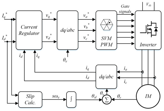
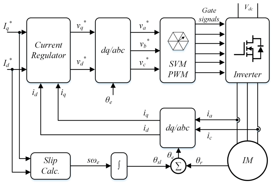
Figure 1 shows the block diagram of the classical indirect FOC. Here, the three-phase currents are measured and transformed to d-q-axis currents using the synchronous angle θ_e, and these $dq$-axis currents are regulated by current regulators that compute the $dq$-axis voltages. To apply these voltages to the IM, inverse-axis transformation calculations are performed, and the reference a-, b-, and c-phase voltages are determined. Calculated phase voltages are then fed to the SVPWM block to generate the required phase voltage waveforms. This conventional FOC structure is used as the reference controller in this paper. In the proposed OEW drive, the same FOC algorithm is retained.

Figure 1. Field-oriented control block diagram of IM.

3. Open-End Winding Drive Structure

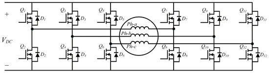
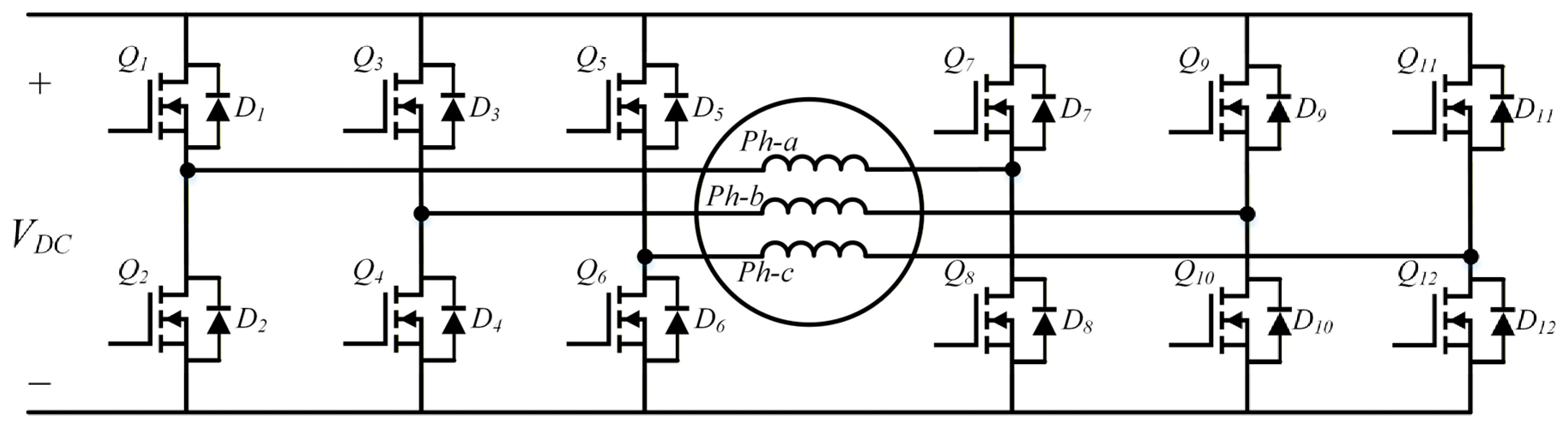
The IM considered in this work employs an OEW stator, in which the neutral point is not internally connected, and both ends of each phase winding are accessible. Accordingly, the stator phase windings are brought out as terminal pairs $(a_1,a_2)$, $(b_1,b_2)$, and $(c_1,c_2)$, corresponding to phases $a$, $b$, and $c$, respectively. This configuration differs from the conventional star- or delta-connected stator, where at least one end of each phase is electrically tied to a common node, as shown in Figure 2. Since all H-bridges share the same DC source, a zero-sequence current path exists through the winding terminals and the DC link; this aspect is analyzed in Section 5.4. By exposing both ends of each phase, the open-end winding structure enables direct per-phase actuation, allowing the external power stage to independently synthesize the phase-to-phase voltage applied to each winding. In the proposed drive, each stator phase is therefore treated as an individually driven single-phase load from the inverter perspective, which is a key enabler for compensating phase-impedance imbalance through per-phase voltage shaping.

Figure 2. OEW motor drive topology.

As shown in Figure 2, each phase is controlled by four switches; for example, phase A is controlled by $Q_1,Q_2,Q_7$ and $Q_8$. Hence, each phase winding is driven by a dedicated single-phase H-bridge inverter. The H-bridge associated with the phase $x\in \{a,b,c\}$ is connected to the corresponding winding terminals $(x_1,x_2)$. Each H-bridge is supplied by the same DC source, denoted as $V_{dc}$.

The way the OEW drive structure controls the phase voltages enables independent phase voltage control.

4. Induction Machine Modeling with Unbalanced Phase Impedances

4.1. Stator Impedance Imbalance

The stator impedance imbalance in the scope of this paper can be represented by converting the voltage imbalance equations into the corresponding machine equations by introducing different impedance components. The voltage imbalance can be modeled by decomposing the unbalanced three-phase IM into positive-sequence and negative-sequence components [3]. The transformation from the stationary to the rotating reference frame is given as

$$\left[\begin{array}{c}{f}_{ds}^e\\ f_{qs}^e\end{array}\right]=\underset{T_s^e}{\underbrace{\left[\begin{array}{cc}\cos {\theta }_e& \sin {\theta }_e\\ -\sin {\theta }_e& \cos {\theta }_e\end{array}\right]}}\left[\begin{array}{c}{f}_{ds}^s\\ f_{qs}^s\end{array}\right]$$

(14)

where e denotes that the variables are in the rotating reference frame. To convert from the voltage imbalance model to the stator impedance imbalance model, the stator voltage equations should be modified while keeping the applied voltages balanced.

On the voltage imbalance case, the stator voltage equations in the stationary frame are represented as

$$v_{ds}^s=r_s{i}_{ds}^s+{\displaystyle \frac{d{\lambda }_{ds}^s}{dt}}$$

(15)

$$v_{qs}^s=r_s{i}_{qs}^s+{\displaystyle \frac{d{\lambda }_{qs}^s}{dt}}$$

(16)

For a balanced impedance machine, the inductances are defined as

$$L_{ds}=L_{qs}=L_{ls}+{\displaystyle \frac{3}{2}}{L}_{ms}$$

(17)

$$M_d=M_q={\displaystyle \frac{3}{2}}{L}_{ms}$$

(18)

On voltage imbalance, the unbalanced inductance parameters are defined as

$$v_{ds}^s=r_{sd}{i}_{ds}^s+L_{lsd}{\displaystyle \frac{d{i}_{ds}^s}{dt}}+M_d{\displaystyle \frac{d}{dt}}\left(i_{ds}^s+i_{dr}^s\right)$$

(19)

$$v_{qs}^s=r_{sq}{i}_{qs}^s+L_{lsq}{\displaystyle \frac{d{i}_{qs}^s}{dt}}+M_q{\displaystyle \frac{d}{dt}}\left(i_{qs}^s+i_{qr}^s\right)$$

(20)

where the impedance imbalance is characterized by $r_{sd}\ne r_{sq}$ (different stator resistances) $L_{lsd}\ne L_{lsq}$ (different leakage inductances). The flux linkage equations under impedance imbalance can be expressed as

$${\lambda }_{ds}^s=L_{ds}{i}_{ds}^s+M_d{i}_{dr}^s=\left(L_{lsd}+L_{md}\right)i_{ds}^s+M_d{i}_{dr}^s$$

(21)

$${\lambda }_{qs}^s=L_{qs}{i}_{qs}^s+M_q{i}_{qr}^s=\left(L_{lsq}+L_{mq}\right)i_{qs}^s+M_q{i}_{qr}^s$$

(22)

where $L_{md}$ and $L_{mq}$ are the d-q axis magnetizing inductances.

Further, the forward–backward transformation for impedance imbalance is observed. Applying the same transformation matrix $\left[T_s^e\right]$ to the impedance-imbalanced equations yields.

• Forward Components (+e):

$$v_{ds}^{+e}=r_s^{+}{i}_{ds}^{+e}+L_s^{+}{\displaystyle \frac{d{i}_{ds}^{+e}}{dt}}+M^{+}{\displaystyle \frac{d}{dt}}\left(i_{ds}^{+e}+i_{dr}^{+e}\right)-{\omega }_e{L}_s^{+}{i}_{qs}^{+e}-{\omega }_e{M}^{+}{i}_{qr}^{+e}$$

(23)

• Backward Components (−e):

$$v_{ds}^{-e}=r_s^{-}{i}_{ds}^{-e}+L_s^{-}{\displaystyle \frac{d{i}_{ds}^{-e}}{dt}}+M^{-}{\displaystyle \frac{d}{dt}}\left(i_{ds}^{-e}+i_{dr}^{-e}\right)+{\omega }_e{L}_s^{-}{i}_{qs}^{-e}+{\omega }_e{M}^{-}{i}_{qr}^{-e}$$

(24)

where the equivalent parameters are presented in Table 1.

Table 1. Equivalent parameters of IM.

Parameter	Forward (+)	Backward (−)
$r_s^{\pm }$	${\displaystyle \frac{r_{sd}+r_{sq}}{2}}$	${\displaystyle \frac{r_{sd}-r_{sq}}{2}}$
$L_s^{\pm }$	${\displaystyle \frac{L_{ds}+L_{qs}}{2}}$	${\displaystyle \frac{L_{ds}-L_{qs}}{2}}$
$M^{\pm }$	${\displaystyle \frac{M_d+M_q}{2}}$	${\displaystyle \frac{M_d-M_q}{2}}$

Key observations for stator impedance imbalance machine equations can be summarized as the following:

• The voltages are balanced, unlike the voltage imbalance case, but $r_{sd}\ne r_{sq}$, $L_{lsd}\ne L_{lsq}$.
• $M_d=M_q$ (if no open phase)
• $L_{ds}\ne L_{qs}$ due to different $L_{ls}$
• Impedance drops are unequal
• Other machine characteristics are affected. The machine’s equivalent circuit is modified to account for stator impedance imbalance.
• Notable differences in the d-axis equivalent circuit:

  ○

  Stator branch: $r_{sd}+j\omega L_{lsd}$ (instead of common $r_s$)

  ○

  Magnetizing branch: $M_d$ (unchanged if no open phase)

• Notable differences in the q-axis equivalent circuit:

  ○

  Stator branch: $r_{sq}+j\omega L_{lsq}$

  ○

  Magnetizing branch: $M_q$

Also, the electromagnetic torque now becomes

$$T_e={\displaystyle \frac{P}{2}}\left[M_q{i}_{qs}^s{i}_{dr}^s-M_d{i}_{ds}^s{i}_{qr}^s+\left(L_{lsq}-L_{lsd}\right)i_{ds}^s{i}_{qs}^s\right]$$

(25)

The additional term $\left(L_{lsq}-L_{lsd}\right)i_{ds}^s{i}_{qs}^s$ represents the reluctance torque due to impedance imbalance.

4.2. FOC Under Impedance Imbalance

Conventional FOC assumes balanced stator impedances ($r_{sd}=r_{sq}=r_s$, $L_{lsd}=L_{lsq}=L_{ls}$). Under impedance imbalance, these assumptions break down. Table 2 presents the outcomes of the impedance imbalance.

Table 2. Outcomes of the impedance imbalance.

FOC Component	Assumption	Reality Under Imbalance Consequence	Consequence
Decoupling circuit	${L_s}^{\prime }=L_s-M^2/L_r$	${L_{sd}}^{\prime }\ne {L_{sq}}^{\prime }$	Cross-coupling terms remain
Current regulators	Identical PI gains for d-q axes	Different dynamics (${\tau }_{sd}\ne {\tau }_{sq}$)	One axis oscillates, the other lags
Flux estimator	${\widehat{\lambda }}_r=f\left(i_{ds},i_{qs}\right)$ with equal weights	Asymmetric contribution	Flux-angle error $\mathsf{\Delta }{\theta }_e$
Torque estimator	${\tau }_e\propto i_{qs}$ with constant $K_T$	$K_{Td}\ne K_{Tq}$	Torque ripple, wrong feedforward

As stated previously on Equations (23) and (24), stator voltage equations in the rotating frame with impedance imbalance are represented as

$$v_{ds}^e=r_{sd}{i}_{ds}^e+L_{lsd}{\displaystyle \frac{d{i}_{ds}^e}{dt}}-{\omega }_e{L}_{sq}{i}_{qs}^e+M_d{\displaystyle \frac{d}{dt}}\left(i_{ds}^e+i_{dr}^e\right)-{\omega }_e{M}_q{i}_{qr}^e$$

(26)

$$v_{qs}^e=r_{sq}{i}_{qs}^e+L_{lsq}{\displaystyle \frac{d{i}_{qs}^e}{dt}}+{\omega }_e{L}_{sd}{i}_{ds}^e+M_q{\displaystyle \frac{d}{dt}}\left(i_{qs}^e+i_{qr}^e\right)+{\omega }_e{M}_d{i}_{dr}^e$$

(27)

The key observation from these equations is that even with balanced applied voltages, impedance imbalance creates.

• Unequal time constants: ${\tau }_{sd}=L_{sd}/r_{sd}\ne {\tau }_{sq}=L_{sq}/r_{sq}$
• Cross-coupling terms that depend on both $i_{ds}^e$ and $i_{qs}^e$
• Asymmetric back-EMF terms

4.3. Impact on Rotor-Flux Orientation

In conventional FOC, the rotor-flux angle is estimated as

$${\theta }_e=\int {\omega }_e dt=\int \left({\omega }_r+{\displaystyle \frac{M{i}_{qs}^e}{{\tau }_r\left|{\lambda }_r\right|}}\right)dt$$

(28)

Under impedance imbalance, the actual slip frequency becomes

$${\omega }_{slip}={\displaystyle \frac{M_d{i}_{qs}^e}{{\tau }_{rd}\left|{\lambda }_{rd}\right|}}-{\displaystyle \frac{M_q{i}_{ds}^e}{{\tau }_{rq}\left|{\lambda }_{rq}\right|}}\cdot {\displaystyle \frac{L_{lsd}-L_{lsq}}{L_r}}$$

(29)

This causes flux-angle estimation error

$$\mathsf{\Delta }{\theta }_e={\tan }^{-1}\left({\displaystyle \frac{\left(L_{lsq}-L_{lsd}\right)i_{qs}^e}{\left|{\lambda }_r\right|+\left(L_{lsd}-L_{lsq}\right)i_{ds}^e}}\right)$$

(30)

So that the resulting estimated d-axis is not aligned with the actual rotor flux, leading to a loss of decoupling between flux and torque, oscillating torque even with constant-current commands, and reduced maximum torque capability.

The model developed in this section establishes the complete causal chain exploited by the proposed controller: the phase-parameter mismatch of Equations (19) and (20) produces unequal impedance drops under the balanced voltage set commanded by conventional FOC, which manifests as phase–current imbalance, distorted airgap MMF, and a rotor-flux orientation error (Equations (28)–(30)). The balancing strategy presented in Section 5 is derived directly from this model: the per-phase static gains introduced in Equation (32) are the controller-level image of the impedance asymmetry of Equations (19) and (20), and the equilibrium condition of Equation (37) shows that the proposed controller converges precisely to the voltage-scaling set that compensates the modeled mismatch—thereby restoring the balanced-current condition under which the FOC of Section 2 is derived.

5. Proposed OEW Drive with Current Balancing Strategy

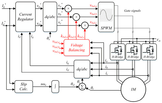
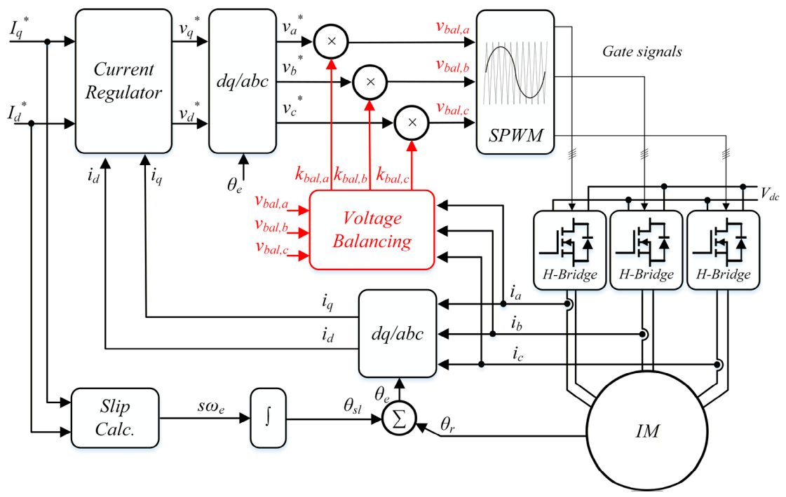
To eliminate the impedance-imbalance-induced problems identified in Section 4, a voltage-balancing controller for the OEW IM drive is proposed, as shown in red in Figure 3. The controller monitors the phase currents and computes their RMS values. If an imbalance among the phase currents is detected, the controller adjusts the corresponding phase voltage amplitude to equalize all three phases. Owing to the OEW drive unit, which consists of three independently controlled H-bridge inverters, the phase voltage amplitudes can be adjusted independently. Unlike a conventional three-leg inverter, all H-bridge inverters are modulated with sine PWM (SPWM); hence, the DC-bus voltage is fully utilized for every phase, and no common-mode injection is introduced by the modulator.

Figure 3. Proposed OEW IM FOC with voltage balancing.

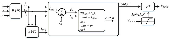
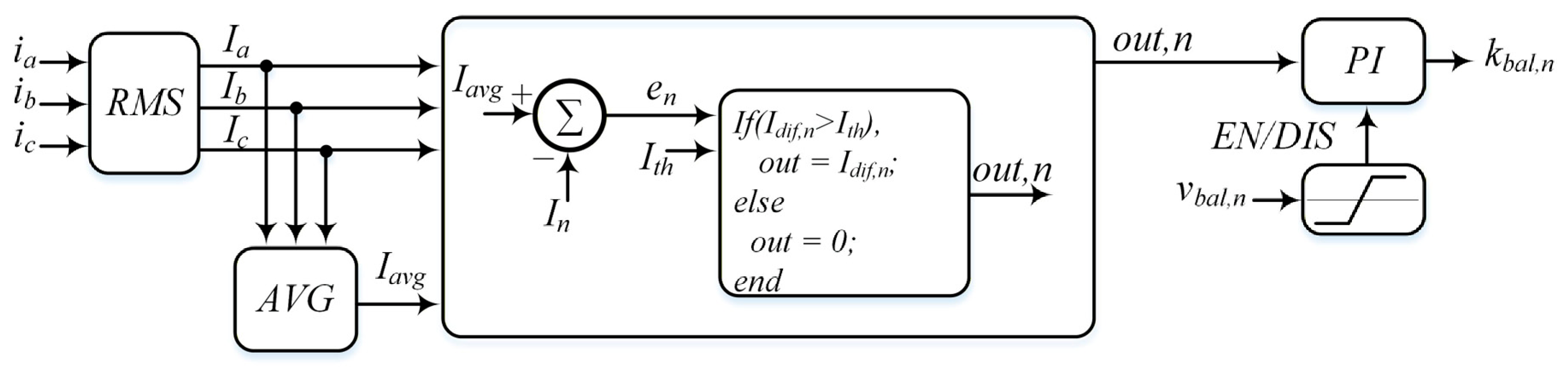
The controller block diagram is shown in Figure 4. First, the RMS values of the phase currents, I_a, I_b, I_c, and their average, I_avg, are computed. For each phase, the deviation in its RMS current from the average, e_n is evaluated; if the deviation exceeds a set threshold, I_th, balancing for that phase is enabled and the deviation is fed to a PI regulator for the n_th phase; otherwise, the regulator input is held at zero and its integrator is frozen. The regulator output is the scaling coefficient k_bal,n that adjusts the phase voltage amplitude. The scaled voltage v_bal,n is also supervised: the integrator is disabled (anti-windup) whenever v_bal,n would exceed the DC-bus voltage, ensuring the modulator always remains within its linear range.

Figure 4. Proposed voltage-balancing algorithm.

The remainder of this section formalizes the control law and links it to the imbalance model of Section 4 in Section 5.1, establishes the stability of the cascaded structure through a bandwidth-separation analysis in Section 5.2, examines the interaction with the FOC framework in Section 5.3, and discusses the zero-sequence behavior of the common-DC-bus OEW topology in Section 5.4.

5.1. Derivation of the Voltage-Balancing Law and Convergence Analysis

Because each stator phase is driven by a dedicated H-bridge, the voltage effectively applied to phase n is the FOC reference voltage scaled by the balancing coefficient:

$$v_{\mathrm{bal},n}(t)=k_{\mathrm{bal},n}(t)\times v_n^{*}(t), n\in \{a,b,c\}$$

(31)

Consider a fixed operating point, i.e., constant speed and load enforced by the inner FOC loops, so that the reference set $v_n^{*}$ is balanced with RMS amplitude $V_{rms}^{*}$. In steady state, the fundamental-frequency RMS current of phase n is then

$$I_n={\displaystyle \frac{k_{\mathrm{bal},n}\times V_{\mathrm{rms}}^{*}}{|Z_n(j{\omega }_e)|}}\triangleq k_{\mathrm{bal},n}\times g_n$$

(32)

where g_n is a static, operating-point-dependent gain that lumps the relation between the applied phase voltage amplitude and the resulting steady-state RMS current, and $|Z_n(j{\omega }_e)|$ is the magnitude of the per-phase input impedance at the operating slip s₀, i.e., $Z_n(j{\omega }_e)=R_n+j{\omega }_e\cdot L_{\mathrm{ls},n}+\left[j{\omega }_e\cdot L_m\parallel \left(R_r/s_0+j{\omega }_e\cdot L_{\mathrm{lr}}\right)\right]$, whose stator branch contains the mismatched resistance R_n and leakage inductance L_ls,n modeled in Section 4.1 (Equations (19) and (20)). The imbalance mechanism identified in Section 4—unequal impedance drops under a balanced voltage set—therefore reappears at the controller level as unequal static gains, g_a ≠ g_b ≠ g_c, which is precisely what the proposed loop acts upon.

The balancing error of phase n is defined with respect to the average RMS current,

$$e_n=I_{\mathrm{avg}}-I_n, I_{\mathrm{avg}}={\displaystyle \frac{I_a+I_b+I_c}{3}}$$

(33)

so that a phase carrying less than the average current receives a coefficient larger than unity, and vice versa. Outside the deadband |e_n| > Ith, the coefficient follows the PI law

$$k_{\mathrm{bal},n}(t)=1+K_p\times e_n(t)+K_i\times {\displaystyle \int e_n}(\tau )d\tau$$

(34)

with the integrator held whenever |e_n| ≤ Ith (to prevent noise in the RMS estimate from producing limit cycles) or whenever v_bal,n reaches the DC-bus voltage limit (anti-windup).

Convergence of the three coupled loops. Since all three errors are referenced to the common average, the loops are not independent; their coupling must be analyzed jointly. Stacking the phase quantities into vectors I = [I_a I_b I_c]^T, k = [k_bal,a k_bal,b k_bal,c]^T, e = [e_a e_b e_c]^T, and using (32) in the form I = G·k with G = diag(g_a, g_b, g_c), the error vector reads

$$e=-P\cdot G\cdot k, P\triangleq I_3-{\displaystyle \frac{1}{3}}\times 1\times 1^{\mathrm{T}}$$

(35)

where 1 = [1 1 1]^T and P is the (symmetric, idempotent) projection matrix onto the zero-average subspace, with eigenvalues {0, 1, 1}. For the slow outer loop, the integral action dominates, $\dot{\mathrm{k}}$ = Ki·e, and differentiating (35) yields the error dynamics

$$\dot{e}=-K_i\cdot P\cdot G\cdot e$$

(36)

Since e = −P·G·k by construction, the error always lies in the range of P, i.e., P·e = e. Taking V = ½·e^Te as a Lyapunov function, its derivative along (36) is $\dot{V}=-K_i\cdot e^{\mathrm{T}}P\cdot G\cdot e=-K_i\cdot {(P\cdot e)}^{\mathrm{T}}G\cdot e=-K_i\cdot e^{\mathrm{T}}G\cdot e=-K_i\cdot {\displaystyle \sum g_n\cdot e_n^2}$, which is strictly negative for any e ≠ 0 because g_n > 0. The error therefore converges exponentially to zero down to the deadband Ith, with a dominant time constant of approximately 1/(Ki·ḡ), where ḡ is the mean of the g_n. The zero eigenvalue of P corresponds to the common-mode direction along one, i.e., a uniform scaling of all three coefficients; this direction is intentionally left uncontrolled by the balancer because the average current amplitude is already regulated by the inner FOC current loops. The proposed controller thus only redistributes current among the phases and, by construction, cannot conflict with the torque- and flux-producing current regulation.

At the equilibrium e = 0, all phases carry the same RMS current, I_n = I_avg, and (32) implies

$${\displaystyle \frac{k_{\mathrm{bal},i}}{k_{\mathrm{bal},j}}}={\displaystyle \frac{g_j}{g_i}}={\displaystyle \frac{|Z_i(j{\omega }_e)|}{|Z_j(j{\omega }_e)|}}$$

(37)

i.e., the balancing coefficients self-scale to mirror the phase-impedance mismatch of Equations (19) and (20) exactly, without any explicit estimation of R_n or L_n. Equation (37) makes the connection between the imbalance model of Section 4 and the proposed controller explicit: the controller converges to the unique voltage-scaling set that compensates the modeled impedance asymmetry, and the residual imbalance is bounded by the user-set threshold I_th.

5.2. Stability and Bandwidth-Separation Analysis

The proposed structure is a cascade: a fast inner FOC current loop and a slow outer RMS-balancing loop. Its stability is assessed using the standard frequency-separation argument for cascade control. In the inner loop, the synchronous-frame PI current regulators run at T_s = 100 µs (K_p = 10, K_i = 1000), yielding an open-loop crossover frequency of 262 Hz, an 81° phase margin, and a closed-loop bandwidth of f_bw,i ≈ 340 Hz. For the outer-loop analysis, the inner closed loop is well approximated by a first-order lag,

$$G_{\mathrm{cl}}(s)\approx {\displaystyle \frac{1}{{\tau }_i\times s+1}}, {\tau }_i={\displaystyle \frac{1}{2\pi \times f_{\mathrm{bw},i}}}$$

(38)

In the outer-loop, the RMS value of each phase current is computed with a moving-average window of one fundamental electrical period, T_w = 1/f_e, which is 60 ms at 500 rev/min, 30 ms at 1000 rev/min, and 20 ms at 1500 rev/min, whose transfer function and low-frequency delay approximation are

$$G_w(s)={\displaystyle \frac{1-e^{-s\times T_w}}{s\times T_w}}\approx e^{-s\times T_w/2}$$

(39)

The outer-loop output is updated every T_u = 100 ms and held constant in between; the zero-order hold contributes an additional equivalent delay of half the update period,

$$G_h(s)\approx e^{-s\times T_u/2}$$

(40)

Combining the PI regulator of (34), the static gain g_n of (32), and the elements above, the open-loop transfer function of one balancing channel evaluated on the zero-average subspace, where the loop gain is g_n per Section 5.1, is

$$L_o(s)=\left(K_p+{\displaystyle \frac{K_i}{s}}\right)\times g_n\times G_{\mathrm{cl}}(s)\times G_w(s)\times G_h(s)$$

(41)

Design criterion. At the 500 rev/min test point, the equivalent-circuit gains evaluate to ḡ ≈ 3.0–3.2 A per unit of k_bal, nearly independent of the load level, since the input impedance is dominated by the magnetizing branch at low slip. The outer-loop gains are K_p = 0.02 and K_i = 0.2, placing the crossover frequency at f_c,o ≈ Ki·ḡ/(2π) ≈ 0.10 Hz, which satisfies

$$f_{\mathrm{c},o}\le {\displaystyle \frac{f_{\mathrm{bw},i}}{100}}$$

(42)

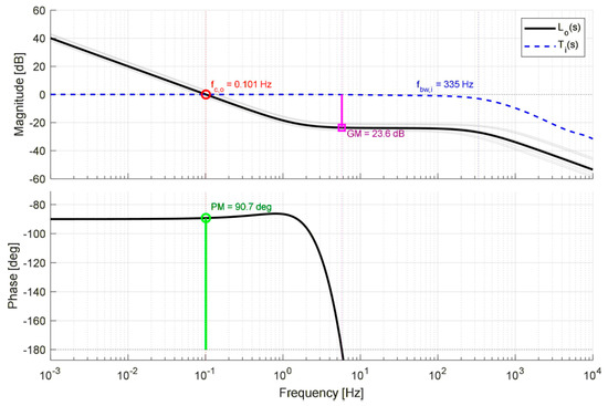
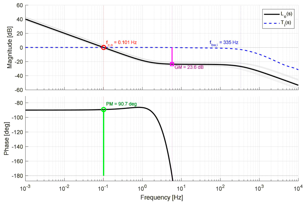
with a large margin: the actual separation is f_bw,i/f_c,o ≈ 3.3 × 10³, which is about 3.5 decades. The 100 ms update period is therefore not an empirical choice but an analytical consequence of (42): with f_c,o ≈ 0.10 Hz, the closed-loop time constant of the balancing loop is 1/(Ki·ḡ) ≈ 1.6 s, so the 10 Hz update rate samples the outer loop about 16 times per time constant, while the delays of (39) and (40) consume only ≈3° of phase at crossover. Figure 5 shows the Bode plot of Lo(s), yielding a gain margin of 24 dB and a phase margin of 90.7°. The solid black curve is the nominal outer open-loop gain L_o(s), and the dashed blue curve is the inner closed-loop response T_i(s); the grey curves show the outer loop under ±30% perturbation of all machine resistances and inductances across the 500–1500 rev/min range. Red markers indicate the outer-loop gain crossover (f_c,o) and the corresponding phase margin (green, lower panel), while the magenta markers denote the −180° crossing and the associated gain margin. Vertical dotted lines mark f_c,o (red), and the inner-loop bandwidth f_bw,i (blue).

Figure 5. Bode plot L_o(s) with parameter perturbations.

To demonstrate robustness against motor-parameter variation, the analysis is repeated with all resistances (R_s, R_r) and inductances (L_ls, L_lr, L_m) perturbed by ±30% of their nominal values, and with the operating slip varied from no load to rated load; over the entire envelope, the crossover moves only between 0.08 and 0.15 Hz, the phase margin remains at ≈91°, and the gain margin stays above 20 dB, confirming stable operation of both loops across the expected parameter range.

Speed dependence. Repeating the analysis at 500, 1000, and 1500 rev/min under constant V/f shows that the loop gain is essentially speed-independent: the phase voltage amplitude and the (inductance-dominated) input impedance both scale with ω_e, so ḡ remains within 3.2–3.4 A per unit, giving f_c,o = 0.104–0.107 Hz, a phase margin of ≈91°, and a gain margin of ≈23 dB at all three speeds; the margins in fact improve marginally with speed because the RMS window T_w = 1/f_e shortens from 60 ms to 20 ms. The operating limit of the method is therefore not stability but actuation authority: the per-phase amplitude boost is bounded by k_max = V_dc/(√2·$V_{rms}^{*}$), which evaluates to ≈5.2, ≈2.6, and ≈1.75 at the three test speeds—far above the required boost of only |Z_a|/|Z_b| ≈ 1.02–1.04—and shrinks toward unity only deep in the field-weakening region, where the anti-windup supervision of Section 5.1 gracefully freezes the balancer at the voltage limit. This is consistent with the flux-weakening extension deferred to future work in the Conclusions section. Finally, combining the speed sweep with the ±30% parameter perturbation—27 cases in total, covering simultaneous speed change and machine-parameter uncertainty—leaves the worst-case margins at a phase margin of 90.6° and a gain margin of 20.4 dB, with f_c,o confined to 0.08–0.15 Hz throughout.

5.3. Interaction with the FOC Framework

As shown in Figure 3, the balancing coefficients act on the phase voltage references after the inverse Park/Clarke transformation; the dq-frame control law itself is left untouched. Their effect on the FOC structure is best seen by decomposing the coefficient vector into common-mode and differential parts,

$$k=\overline{k}\times 1+\mathsf{\Delta }k, \overline{k}={\displaystyle \frac{k_{\mathrm{bal},a}+k_{\mathrm{bal},b}+k_{\mathrm{bal},c}}{3}}$$

(43)

The common-mode part $\overline{k}$ scales all three-phase voltages equally and is therefore indistinguishable, from the dq frame, and from a slow variation in the effective DC-bus gain; the inner current regulators absorb it exactly as they absorb bus-voltage sag, well within their ≈340 Hz bandwidth. The differential part Δk introduces an intentional asymmetric (negative-sequence) voltage component at the fundamental frequency, dimensioned by the outer loop to cancel the negative-sequence current caused by the impedance asymmetry of Equations (19) and (20). In other words, the balancer restores the balanced-current condition under which the rotor-flux orientation of Equation (28) and the dq-axis decoupling are derived, rather than perturbing them: as the negative-sequence current content shrinks, the flux-angle estimation error of Equation (30) is reduced accordingly.

Two time-scale properties guarantee non-interference. First, the outer loop evolves with a bandwidth of ≈0.1 Hz and is updated at 10 Hz, i.e., more than three orders of magnitude below the inner current-loop bandwidth; from the perspective of the 100 µs inner loop, k_bal,n is quasi-static. Second, the anti-windup supervision of Section 5.1 keeps v_bal,n within the DC-bus limit, so the SPWM modulator remains in its linear range and the inner-loop plant gain is never distorted by overmodulation. Consequently, rotor-flux orientation, dq decoupling, and the inner-loop stability margins established in Section 5.2 are preserved throughout balancing transients.

5.4. Zero-Sequence Considerations in the Common-DC-Bus OEW Topology

Since all three H-bridges are supplied by the same DC source (Figure 2), a zero-sequence current path exists through the winding terminals, the six half-bridge legs, and the DC link—a well-known property of common-DC-bus OEW drives [21,22]. Three excitation sources must be distinguished. First, modulation: because each H-bridge is driven by per-phase SPWM without any common-mode or third-harmonic injection, the modulator itself introduces no intentional low-frequency zero-sequence voltage, unlike SVPWM-based dual-inverter schemes [14]. Second, machine and converter non-idealities: back-EMF harmonics and dead-time effects excite a residual high-frequency zero-sequence component, common to all common-DC-bus OEW drives [21,23]. Third, the proposed balancer itself: deliberately unequal amplitude scaling produces a fundamental-frequency zero-sequence voltage component:

$$v_0={\displaystyle \frac{v_{\mathrm{bal},a}+v_{\mathrm{bal},b}+v_{\mathrm{bal},c}}{3}}={\displaystyle \frac{1}{3}}\times {\displaystyle \sum _n(k_{\mathrm{bal},n}-1)}\times v_n^{*}$$

(44)

whose magnitude is proportional to the spread of the balancing coefficients—a few percent of the phase voltage for realistic manufacturing-induced mismatch. It should be emphasized, however, that under phase-impedance imbalance, a zero-sequence current component ((i_a + i_b + i_c)/3 ≠ 0) already circulates before any compensation is applied, since the unequal phase currents do not sum to zero. The relevant question is therefore whether balancing amplifies this circulating component. The experimental results in Section 6 include the measured sum i_a + i_b + i_c before and after enabling the balancer, showing that the zero-sequence content is not increased—the fundamental-frequency asymmetric voltage of (44) replaces, rather than adds to, the pre-existing zero-sequence excitation caused by the current imbalance itself. A dedicated zero-sequence controller, e.g., along the lines of [10,14], is orthogonal to the proposed method and can be combined with it; however, this extension falls outside the scope of this work. It is also worth noting that this consideration is specific to the common DC-bus configuration studied here: if the three H-bridges are instead supplied from galvanically isolated DC sources or batteries, no zero-sequence current path exists, and the above concern is eliminated altogether.

Table 3 compares the proposed scheme with the main families of imbalance-mitigation techniques discussed in Section 1. Since the targeted impedance mismatch is set at manufacturing and is essentially time-invariant, a fast compensation loop is neither required nor desirable. Hence, the dynamic response of the drive remains the same as that of the underlying FOC. What distinguishes the proposed method is that it requires neither parameter estimation nor additional hardware, while retaining full per-phase actuation authority through the OEW structure, which is a combination that the single-inverter methods cannot provide.

Table 3. Comparison of phase–current imbalance-mitigation approaches.

Method	Parameter Estimation	Extra Hardware	Steady-State Limit
Sequence-component compensation [3,4]	No	No	Sequence-extraction accuracy
Online parameter estimation [1,2]	Yes	No	Estimate accuracy
External hardware compensation [6]	No	Yes	Design point only
Proposed RMS-based OEW balancing	No	No	Deadband Ith

6. Results and Discussions

To validate the proposed system’s efficacy, simulations in MATLABR2024b/Simulink and laboratory experiments were conducted. This section includes details on the test rig and measurement devices, simulation results, and experimental validation.

6.1. Test Setup

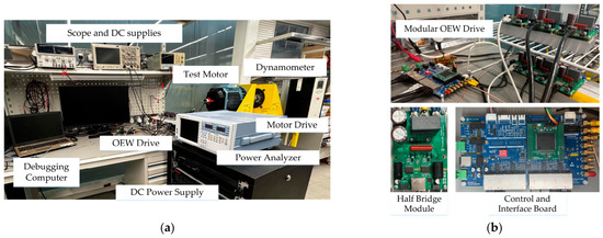
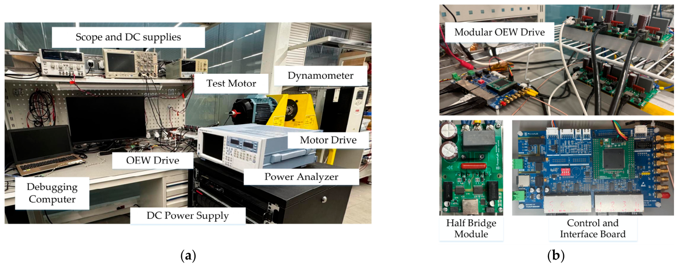
The test system shown in Figure 6a consists of a dynamometer capable of operating in all four quadrants up to 5 kW with an ABB ACS 880 regenerative drive unit. Torque and speed measurements were done with a 50 Nm ETH-Technik torque transducer and a Yokogawa WT1800 series power analyzer. Phase currents were measured with Fluke 80i–110 s current probes and a Tektronix MDO 3014 100 MHz oscilloscope. An Ametek-Sorensen SGX Series DC power supply was used to power the motor drive. The modular OEW drive system comprises six half-bridge modules, three current-sensing modules, and a control and interface board. The control is performed with the TI TMS320F28386D triple-core digital signal processor.

Figure 6. (a) Complete test setup and (b) modular OEW drive system.

6.2. Simulation Results

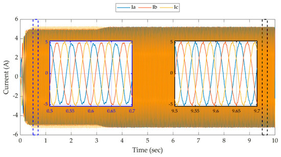
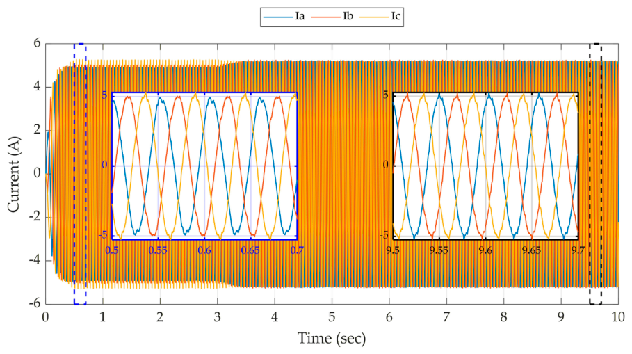
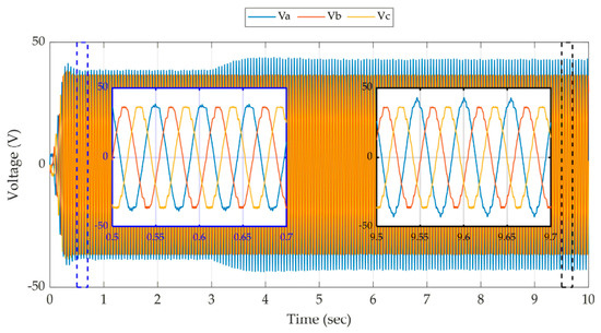
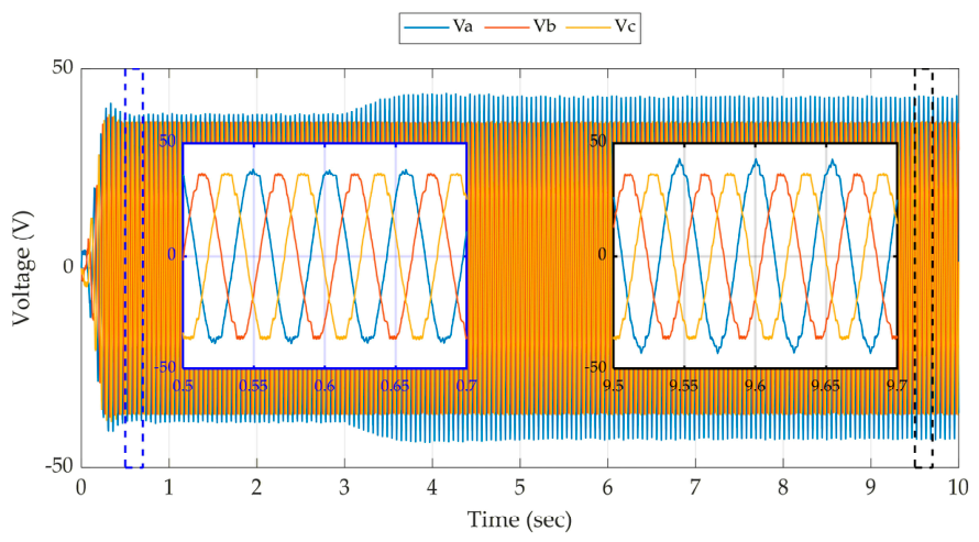
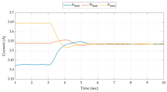
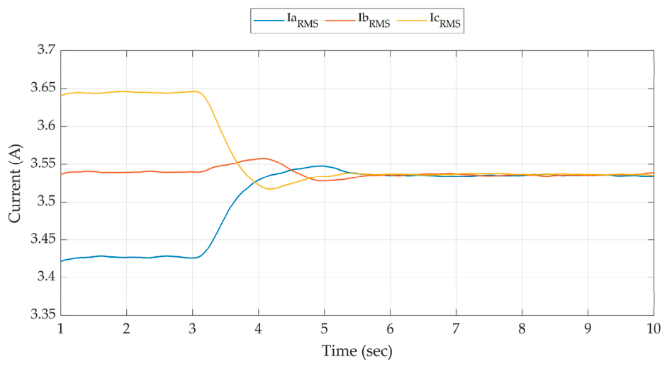
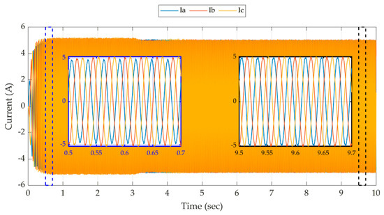
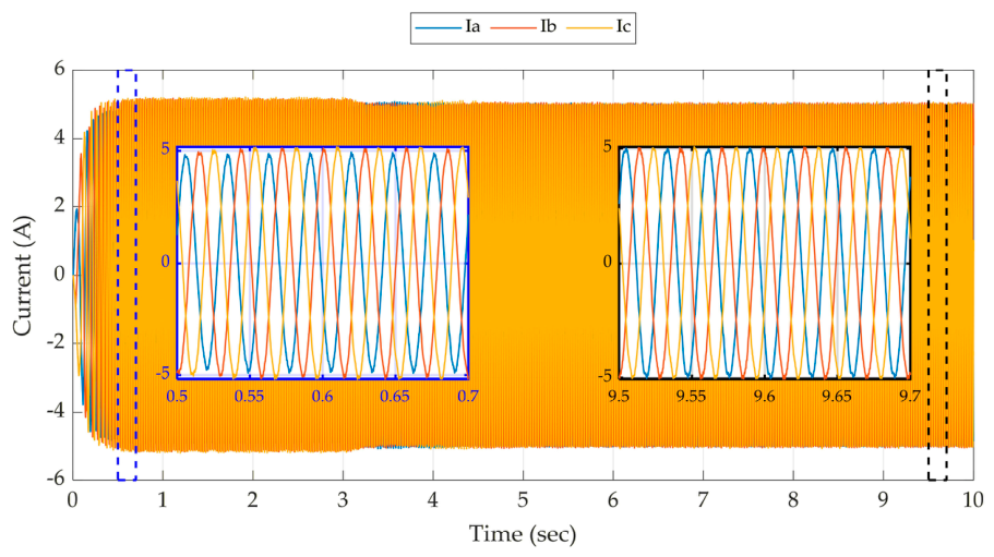
Simulations are performed under the MATLAB/Simulink environment. The machine used in this study is a four-pole, IE2-class 5.5 kW ABB IM, modeled in Simulink. The simulation step time is set to 1 µsec, and the simulation time to 10 s. To test the impedance imbalance, an additional RL impedance is added to phase A of the machine, and classical FOC begins controlling the phase currents while the balancing algorithm is inactive. Later, the balancing algorithm is enabled at the third second, and the variations in the phase currents, their RMS values, and reference voltage waveforms are observed under the same loading condition at 500 and 1000 rev/min.

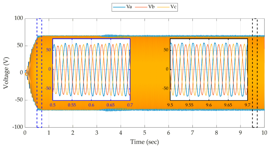
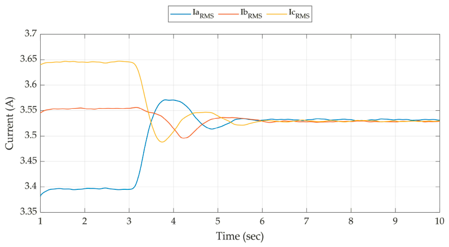
The simulation results are presented in Figure 7, Figure 8, Figure 9, Figure 10 and Figure 11. In Figure 7, the instantaneous phase currents are shown. Here, the figure is zoomed in to show the current imbalance at the 0.5th second. After the current balancing control is enabled at the third second, the imbalance is reduced to 0.05 A, the threshold value. The figure zoomed in again at the 9.5th second to observe that balanced phase currents. Similar observations are made at the specified time frames for the reference-phase voltages and the RMS current, as shown in Figure 8 and Figure 9, respectively.

Figure 7. Phase currents before and after current balancing at 500 rev/min.

Figure 8. Reference-phase voltages before and after current balancing at 500 rev/min.

Figure 9. RMS phase currents before and after current balancing at 500 rev/min.

Figure 10. Phase currents before and after current balancing at 1000 rev/min.

Figure 11. Reference-phase voltages before and after current balancing at 1000 rev/min.

Simulations are repeated at 1000 rev/min for the current amplitude condition, and the results are presented in Figure 10, Figure 11 and Figure 12.

Figure 12. RMS phase currents before and after current balancing at 1000 rev/min.

6.3. Experimental Results

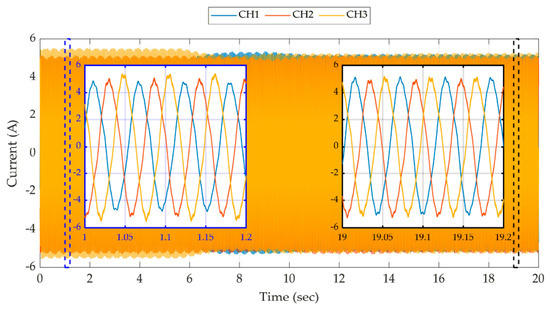
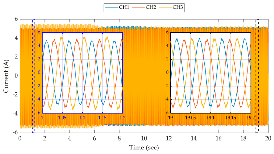
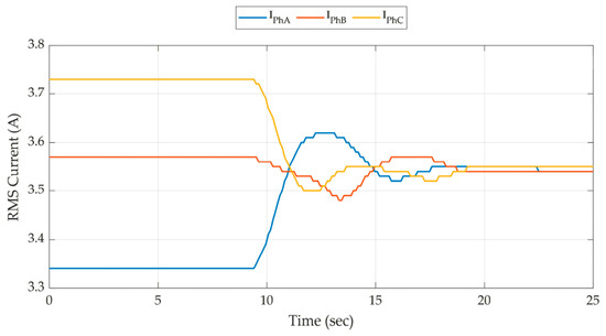
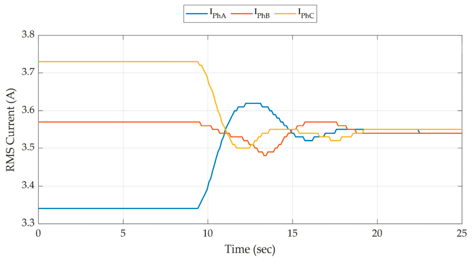
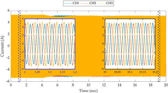
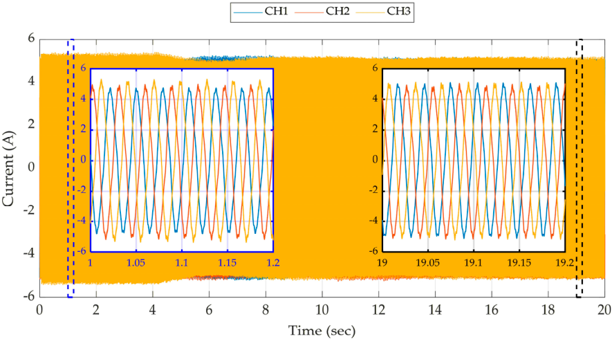
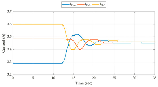
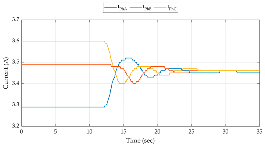
The FOC and current balancing system are implemented on a digital signal processor, and the system is tested under the same speed and loading conditions. The impedance imbalance is externally added to the system via an inductor with 2 mH inductance and 0.7 Ω resistance. The system is started with balancing control disabled. Later, it is enabled manually, and instantaneous and RMS current waveform variations are captured from the oscilloscope. Figure 13 shows the captured instantaneous current waveforms, and Figure 14 shows the RMS values of these currents. Figure 15 and Figure 16 present the corresponding waveforms and RMS values at 1000 rev/min. At the beginning of the experiment, the currents are not balanced. After enabling the balancing control, their amplitudes approach the commanded current value by the FOC. Here, the selection of the PI coefficients determines how fast and oscillatory the response will be. For this study, the proportional and integral coefficients are set to 0.02 and 0.2, respectively.

Figure 13. Experimental phase currents before and after current balancing at 500 rev/min.

Figure 14. Experimental RMS phase currents before and after current balancing at 500 rev/min.

Figure 15. Experimental phase currents before and after current balancing at 1000 rev/min.

Figure 16. Experimental RMS phase currents before and after current balancing at 1000 rev/min.

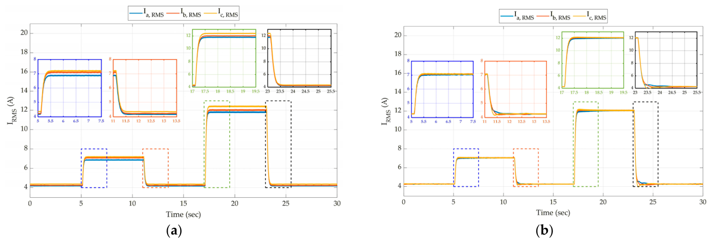
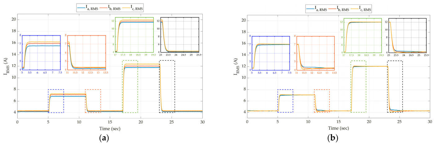
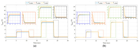
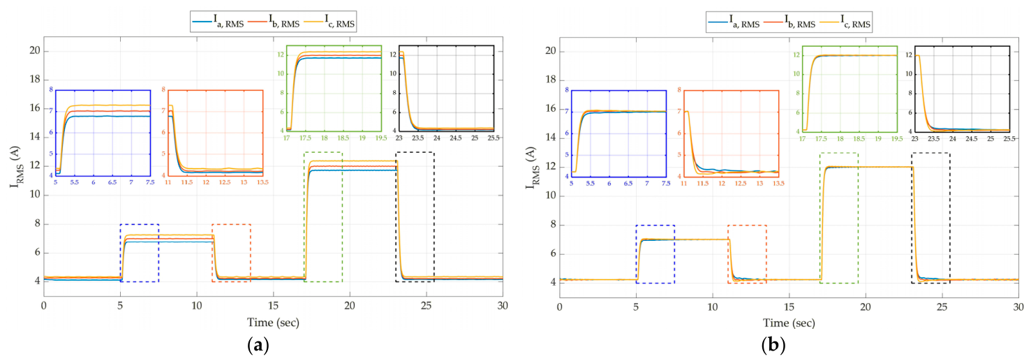
To assess the balancing performance over the full operating envelope, a complete loading profile—0% → 50% → 0% → 100% of the rated torque—is applied at 500, 1000, and 1500 rev/min, with the balancing controller enabled, and is repeated with the controller disabled for reference. Figure 17, Figure 18 and Figure 19 present the phase RMS currents along the profile at each speed. The d-axis current is set to 6 A rated value, and the q-axis current is varied stepwise from 0 to 8 A and 16 A levels, which corresponds to 50% and 100% rated loading conditions.

Figure 17. RMS phase currents variation when loaded (a) with and (b) without current balancing at 500 rev/min.

Figure 18. RMS phase currents variation when loaded (a) with and (b) without current balancing at 1000 rev/min.

Figure 19. RMS phase currents variation when loaded (a) with and (b) without current balancing at 1500 rev/min.

The phase currents remain balanced at every load level and re-converge after each load transition within a few outer-loop time constants, in agreement with the ≈1.6 s constant predicted in Section 5, while the dq-axis currents follow their references without observable disturbance from the balancing action, confirming the non-interference analysis.

The imbalance index (IU), defined as the maximum difference between the average current and the maximum deviation from the average current, and the zero-sequence current I₀ are adopted as quantitative metrics because they directly capture the fundamental-frequency amplitude asymmetry caused by a linear impedance mismatch. Such a mismatch does not generate harmonic distortion, so the phase–current THD remains essentially unchanged; likewise, the associated torque ripple should appear at twice the fundamental frequency, which is beyond the bandwidth of the in-line torque sensor. Since the artificially added impedance is external to the machine, the stator-winding copper loss of each phase is proportional to the square of the current, and the equalization of the RMS currents in Table 4 directly equalizes the internal copper-loss distribution.

Table 4. Measured current imbalance index and zero-sequence current RMS over the loading profile, with the balancing controller disabled (Off) and enabled (On).

Speed (rev/min)	Load (%)	Current Imbalance IU (%)		Zero-Sequence I0 RMS (A)
		Balancer Off	Balancer On	Balancer Off	Balancer On
500	0	2.58	<0.1	0.11	0.01
	50	1.94	<0.1	0.14	0.05
	100	2.76	<0.1	0.35	0.06
1000	0	2.04	<0.1	0.12	0.03
	50	2.93	<0.1	0.16	0.05
	100	2.63	<0.1	0.24	0.05
1500	0	2.43	<0.1	0.07	0.04
	50	3.61	<0.1	0.11	0.06
	100	2.66	<0.1	0.19	0.06

Table 4 summarizes the measured imbalance index and zero-sequence current RMS for various speed and loading conditions, with the balancing controller disabled and enabled. When it is disabled, these operating conditions span a range of imbalance conditions, IU = 1.94–3.61% and I₀ = 0.07–0.35 A, reflecting the combined effect of the fixed external impedance and the varying slip and voltage across the test matrix. At rated load specifically, the zero-sequence current decreases with speed—0.35 A, 0.24 A, and 0.19 A at 500, 1000, and 1500 rev/min, respectively—even though the external imbalance is unchanged, consistent with the reduction in the effective impedance–mismatch ratio predicted analytically in Section 5.4. When the balancing controller is enabled, the current imbalance index is almost zero at every operating point, with the residual bounded by the deadband threshold, Ith. Also, the zero-sequence current is almost completely eliminated for every operating point. Since balanced equal-amplitude currents sum to zero, the balancing controller actively suppresses the circulating component.

7. Conclusions

AC machines often exhibit phase-to-phase impedance imbalance due to manufacturing tolerances and winding-layout variations, even when the phase windings have the same number of turns by design. This work proposes a phase–current-balancing method that leverages the open-end-winding (OEW) motor drive’s independent voltage control feature. The method is applicable to any motor control topology utilizing output phase voltages as the control variable, regardless of the specific control method. The current balancing algorithm monitors the phase RMS currents and adjusts the output voltage reference amplitudes to balance the phase currents. The effect of the imbalance is analyzed mathematically for the FOC IM drive, and it is observed that the imbalanced phase currents cause torque oscillations, vibrations, and inefficient operation. In this work, an induction machine (IM) with a classical field-oriented controller (FOC) drive system is considered. Externally added RL impedance is applied to one phase to create an imbalance in phase impedance and the phase currents, and test the efficacy of the proposed balancing method. The system is simulated in MATLAB/Simulink and experimentally validated at 500, 1000, and 1500 rev/min under the same loading conditions. Across various speed and loading conditions, spanning a current imbalance index of 1.94–3.61% and a zero-sequence current of 0.07–0.35 A, the proposed controller almost completely eliminated the imbalance and reduced the zero-sequence current to below 0.06 A, without parameter estimation or retuning. Beyond the empirical demonstration, the balancing law was derived from the phase-impedance imbalance model, exponential convergence of the coupled per-phase loops was proven via a Lyapunov argument, and stability of the cascaded structure was established analytically, with a crossover separation of more than three decades from the inner current loop and stability margins shown to be insensitive to ±30% machine-parameter variation and to the operating speed. Since the system operates according to current control principles, any current imbalance at any operating point within the voltage limits can be balanced using the proposed method. The operating limit of the method is set by actuation authority rather than stability: the per-phase amplitude boost is bounded by the DC-bus voltage, a margin that shrinks toward unity deep in the field-weakening region, where the anti-windup supervision freezes the balancer at the voltage limit. Future work may therefore include extending the balancing strategy into the flux-weakening region and maximum-torque-per-voltage operation, together with a dedicated zero-sequence current controller.

References

- Singh, B.P. Real-Time Detection of Stator Resistance Unbalances in Three Phase Induction Motor Drives. Master’s Thesis, KTH Royal Institute of Technology, Stockholm, Sweden, 2020. [Google Scholar]
- Stefani, A. Induction Motor Diagnosis in Variable Speed Drives. Ph.D. Thesis, Alma Mater Studiorum—Università di Bologna, Bologna, Italy, 2010. [Google Scholar]
- Jannati, M.; Idris, N.R.N. Vector Control of Unbalanced 3-Phase IM Using Forward and Backward Components. Turk. J. Electr. Eng. Comput. Sci. 2017, 25, 1358–1374. [Google Scholar] [CrossRef]
- Mohammed, O.M.E.M.; Yang, X.; Zhao, Y. An Improved Control Strategy for Induction Motor under Unbalanced Voltage Source with Torque Loop. Ain Shams Eng. J. 2025, 16, 103738. [Google Scholar]
- Von Jouanne, A.; Banerjee, B. Assessment of Voltage Unbalance. IEEE Trans. Power Deliv. 2001, 16, 782–790. [Google Scholar] [CrossRef]
- Hu, Y.; Zhu, Z.Q.; Odavic, M. Compensation of Unbalanced Impedance of Asymmetric Wind Power PMSG Compensated by External Circuits in Series. CES Trans. Electr. Mach. Syst. 2017, 1, 180–187. [Google Scholar] [CrossRef]
- Falsiroli, M. State of the Art and Analysis of Open-End Winding Motor Drives. Master’s Thesis, Politecnico di Milano, Milan, Italy, 2023. [Google Scholar]
- Antivachis, M. Analysis of Double-Bridge Inverters for Drive Systems with Open-End Winding Motors. Ph.D. Thesis, ETH Zurich, Zurich, Switzerland, 2020. [Google Scholar]
- Dong, Z.; Wen, H.; Song, Z.; Liu, C. 3-D SVM for Three-Phase Open-End Winding Drives with Common DC Bus. IEEE Trans. Power Electron. 2023, 38, 12456–12468. [Google Scholar] [CrossRef]
- Dong, Z.; Song, Z.; Wang, W.; Liu, C. Improved Zero-Sequence Current Hysteresis Control-Based Space Vector Modulation for Open-End Winding PMSM Drives with Common DC Bus. IEEE Trans. Ind. Electron. 2023, 70, 10755–10760. [Google Scholar] [CrossRef]
- Hu, W.; Wang, X.; Nian, H.; Sun, D. A Fault-Tolerant Scheme Against the Open-Switch Failure in Open-End Winding PMSM System with Isolated DC bus. IEEE Trans. Energy Convers. 2023, 38, 2021–2030. [Google Scholar] [CrossRef]
- Hu, W.; Ruan, C.; Nian, H.; Sun, D. Simplified Modulation Scheme for Open-End Winding PMSM System with Common DC Bus Under Open-Phase Fault Based on Circulating Current Suppression. IEEE Trans. Power Electron. 2020, 35, 10–14. [Google Scholar] [CrossRef]
- Reddy, K.S.; Baskar, S. A Literature Review on Open-End Windings Induction Motor Drives. In Proceedings of the 5th International Conference on ICEECCOT, Mysuru, India, 10–11 December 2021; pp. 395–398. [Google Scholar]
- Rovere, L.; Formentini, A.; Cox, T.; Lo Calzo, G. Zero-Sequence Voltage Elimination for Dual-Fed Common DC-Link Open-End Winding PMSM High-Speed Starter–Generator—Part I: Modulation. IEEE Trans. Ind. Appl. 2019, 55, 7804–7812. [Google Scholar] [CrossRef]
- Kanaujia, A.K.; Kumar, S. A Novel Multi-level SVPWM Scheme for High Power Induction Motor Drive Applications. In Proceedings of the IEEE ICCC, Dhanbad, India, 28 February–2 March 2025; pp. 1–6. [Google Scholar]
- Osman, R.H. A New Approach to Enhance Power Quality for Medium Voltage AC Drives. IEEE Trans. Ind. Appl. 1997, 33, 204–210. [Google Scholar] [CrossRef]
- Nian, H.; Hu, W.; Ruan, C.; Sun, D. An Improved Modulation Technique with Minimum Switching Actions Within One PWM Cycle for Open-End Winding PMSM System with Isolated DC Bus. IEEE Trans. Ind. Electron. 2020, 67, 198–207. [Google Scholar] [CrossRef]
- Wei, J.; Kong, X.; Zhang, Z.; Zhou, B. Integrated Control Strategy for Distortion Current Elimination of Fault-Tolerant Open-End Winding Permanent Magnet Synchronous Machine with Topology Reconfiguration. IEEE J. Emerg. Sel. Top. Power Electron. 2023, 11, 1541–1554. [Google Scholar] [CrossRef]
- Stolyarov, E.; Fedorova, K.; Ali, Y.; Kulik, E.; Lashkevich, M.; Anuchin, A. Current Regulation in Case of Open Circuit Fault for Six-phase Traction Open-end Winding Machine. In Proceedings of the 2020 IEEE UPEC, Torino, Italy, 1–4 September 2020. [Google Scholar]
- Zhu, B.; Tan, C.; Farshadnia, M.; Fletcher, J.E. Postfault Zero-Sequence Current Injection for Open-Circuit Diode/Switch Failure in Open-End Winding PMSM Machines. IEEE Trans. Ind. Electron. 2019, 66, 5124–5132. [Google Scholar] [CrossRef]
- Somani, A.; Gupta, R.K.; Mohapatra, K.K.; Mohan, N. On the Causes of Circulating Currents in PWM Drives with Open-End Winding AC Machines. IEEE Trans. Ind. Electron. 2013, 60, 3670–3678. [Google Scholar] [CrossRef]
- Hunter, N. Research on the Uncontrolled Zero-Sequence Current of an Open-End Winding PMSM with Common DC Link. Ph.D. Thesis, University of Nottingham, Nottingham, UK, 2020. [Google Scholar]
- Belkhode, S.; Jain, S. Optimized Switching PWM Technique with Common-Mode Current Minimization for Five-Phase Open-End Winding Induction Motor Drives. IEEE Trans. Power Electron. 2019, 34, 8971–8980. [Google Scholar] [CrossRef]
- Raherimihaja, H.J.; Yuan, Z.; Wang, J.; Zhang, Q. A Three-Phase Integrated Battery Charger for EVs Based on Six-Phase Open-End Winding Machine. IEEE Trans. Transp. Electrif. 2020, 6, 1245–1257. [Google Scholar]
- Monteiro, A.P.; Jacobina, C.B.; Bahia, F.A.; Sousa, R.P. Vienna Rectifiers for WECS Applications with Open-End Winding PMSM. IEEE Trans. Ind. Appl. 2022, 58, 2268–2279. [Google Scholar] [CrossRef]
- Cha, K.S.; Kim, J.H.; Hwang, S.W.; Lim, M.S.; Park, S.H. High-Efficiency e-Powertrain Topology by Integrating Open-End Winding and Winding Changeover for Improving Fuel Economy of Electric Vehicles. Mathematics 2024, 12, 3415. [Google Scholar] [CrossRef]
- Chu, L.; Jia, Y.F.; Chen, D.S.; Xu, N.; Wang, Y.W.; Tang, X.; Xu, Z. Research on Control Strategies of an Open-End Winding Permanent Magnet Synchronous Driving Motor (OW-PMSM)-Equipped Dual Inverter with a Switchable Winding Mode for Electric Vehicles. Energies 2017, 10, 616. [Google Scholar] [CrossRef]
Disclaimer/Publisher’s Note: The statements, opinions and data contained in all publications are solely those of the individual author(s) and contributor(s) and not of MDPI and/or the editor(s). MDPI and/or the editor(s) disclaim responsibility for any injury to people or property resulting from any ideas, methods, instructions or products referred to in the content. |
© 2026 by the authors. Licensee MDPI, Basel, Switzerland. This article is an open access article distributed under the terms and conditions of the Creative Commons Attribution (CC BY) license.