EST-GNN: An Explainable Spatio-Temporal Graph Framework with Lévy-Optuna Optimization for CO₂ Emission Forecasting in Electrified Transportation

Abstract

The accurate and explainable prediction of carbon emissions is crucial for the efficient operation of hybrid and electrified transportation systems and their integration with energy grids. An Explainable Spatio-Temporal Graph Neural Network (EST-GNN) is proposed for highly precise CO₂ emission forecasting using Lévy Flight-guided Optuna optimization. By modelling vehicles and their operational characteristics as nodes in a dynamic graph, the proposed framework can jointly learn timing and spatial correlations while sustaining interpretability. The accuracy of the EST-GNN model is compared with models based on one-hot encoded features, SMOTE-enhanced datasets, and ensemble regressors. Using a real-world dataset of 7385 vehicle registrations with 12 predictive features experiments are conducted. When applied the EST-GNN model outperformed all baseline and traditional models achieving the highest reliability (R² = 0.98754) while solving competitive error metrics (RMSE = 6.55, MAE = 2.556). There is strong indication that reasonable machine learning (ML) models can be used accurately to confirm their suitability for resource-prevented and real-time applications, while predictable ML techniques have relatively low reliability. The optimal solution ensures scalability, robustness, and independence of the deployment environment. The distribution analysis of best performing models develops the ability of EST-GNN, which accounts for the largest proportion of best results across evaluation metrics. To achieve superior predictive accuracy, graph-based learning, explainability, and advanced hyperparameter optimization are combined. EST-GNN provides a powerful tool for analyzing fleet emission levels, making energy-aware decisions, and planning sustainable transportation, while ML models continue to be a useful complement for deployment states with high computation costs and quick responses.

1. Introduction

Greenhouse gas emissions, particularly carbon dioxide (CO₂), represent a primary global challenge in the 21st century. Global warming plays a critical role in climate change and greatly influences the socioeconomic systems of many countries. Emissions come from fossil fuel combustion and industrial processes. They are chief sources of human-induced climate change and global warming. These emissions come from a mix of energy, transportation, and industrial sources with activities. Some authors have derived a simplified multi-step framework for CO₂ emissions estimation based on important data such as energy consumption and using clustering, predictive machine learning (ML) algorithms, and feature selection techniques [1]. The authors proposed an approach to choosing the CO₂ predictor for real-time daily emissions in some countries, including China. ML brought to the fore the advances in carbon emission prediction by processing big data better and faster.

In contrast to conventional statistical methods, ML and Deep Learning (DL) techniques can process large amounts of historical and real-time data like energy consumption, industrial production or economic indicators to discover covered patterns and non-linear correlations. In addition, other effective methods such as regression models and neural network methods have also improved the forecasting accuracy so that organizations can estimate emission patterns and come up with measures to mitigate them. It also supplies stakeholders with the capability to make more learned outcomes, since ML can be used to evaluate several environmental procedures that allow the estimation of potential scenarios. ML and DL are also critical for tackling climate change and accelerating environmental growth by automating and improving the estimation of greenhouse gas emissions.

An Explainable Spatio-Temporal Graph Neural Network (EST-GNN) is proposed for highly precise CO₂ emission forecasting using Lévy Flight-directed Optuna optimization in this paper. The rest of this paper is organized as follows: Section 2 introduces the related work and literature review. The system model and methodology are described in Section 3. The experimental findings for each constituent of the proposed model are shown in Section 4. Finally, the paper is summarized and concluded in Section 5.

2. Literature Review

Governments, scientists, and international organizations have prioritized CO₂ reduction through policies such as the Paris Agreement, carbon pricing, and renewable energy adoption. Additionally, advancements in Carbon Capture and Storage (CCS) technologies, along with sustainable energy transitions, are being explored to curb emissions. The industrial emissions data show a discrete spatial and temporal distribution and significant seasonal fluctuation, and the management of industrial production requires high temporal resolution and predictive accuracy. It is worth noting that most of the current regional prediction studies of industrial carbon emissions are implemented based on long-term future predictions (annual or monthly scales), and the short-term high-frequency real-time emission prediction problem based on industrial processes is not discussed. While these studies can accurately model long-term emission pathways and policy scenarios, some authors often do not provide the real-time fidelity that is necessary for deployment in industrial process control.

Real-time monitoring of high-frequency carbon emissions provides vital information regarding industrial practices so that future policymakers can better inform themselves about regional emission dynamics and identify individual high emitters timeously.

Accurate emissions forecasting of future carbon emissions is of enormous significance to sustainable development policies and is the scientific basis for the formulation of effective emission reduction policies. The Yellow River Basin is a significant economic and environmental province, which was listed as one of the key territorial regions in China’s regional development strategy. The analysis of the driving factors of carbon emissions in this area and the establishment of accurate prediction models is important for decision-making during the process of policy. In addition, if the emission reduction in the Yellow River Basin can be strengthened, it will also significantly help to realize China’s dual carbon goals of peaking and carbon neutrality. Authors in [2] were focused on analyzing the nexus between CO₂ emissions, energy consumption and economic growth in Russia with annual time series data from 1970 up to 2017. Initial examination consisted of the use of time series analyses (checking for stationarity, breaks, cointegration, etc.).

An innovative data-to-causality (D2C) algorithm was created and played together with an experiment in machine learning. A comparative calculation of the two approaches revealed that economic growth is a decisive factor of energy consumption and CO₂ emissions. Nevertheless, variance decomposition analysis indicated that positive and sustainable economic growth can be strategically used to prompt investment in other sources of energy with less pollution influence. These results were later verified in robustness checks using the new D2C algorithm. Finally, the presence of causal connections between these variables was verified in temporary economic environments. International climate mitigation campaigns are leading countries to increasingly ambitious greenhouse gas reduction targets. In contrast, there is limited evidence of the causal effects of these targets on the implementation of policies and the allocation of resources. A study applying discontinuity regression analysis in [3] suggested that higher emissions targets in China have a strong effect on the decision of municipal land use; approximately 15% more land has been allocated for carbon-efficient industries in cities with more energy conservation efforts than in areas with weaker targets.

It is important to note that the results showed that these environmental standards reduce the supply of land to carbon-intensive sectors in the same way, indicating that historical economic dependencies and regional comparative advantages continue to exert their influence. The analysis also finds that the strength of the policy efficiency relationship is scoured by economic growth requirements and career advancement motivations for local officials. On the other hand, public environmental awareness was found to increase policy compliance. The study has reported a twin fate in high-carbon goal areas such as simultaneous regressions in emissions and economic activity after shifting land to cleaner industries. These results provide important lessons for the development of multitask governance systems which also consider economic development objectives, particularly in balancing environmental sustainability with economic growth in high-carbon goal areas.

In ref. [4], two main steps of a methodological process were used to calculate the main distributions and reactions to the deployment of CE in support of China’s move towards a carbon-neutral economy. A Fuzzy Analytical Hierarchy Process (FAHP)-based approach is presented in ref. [4]. To mitigate CO₂ emissions from commercial-scale CE options, FAHP was applied to determine the most critical barriers.

Another Fuzzy VIekriterijumsko KOmpromisno Rangarajan (FVIKOR) approach was also used to assess alternative strategic options addressing the identified and reported scenarios, specifically focusing on evaluating their effectiveness in reducing CO₂ emissions and overcoming the barriers highlighted by the FAHP analysis.

The FAHP analysis identified waste management systems as the most crucial challenge (CECER2), followed by regulatory intricacy (CECER5) and lack of financial support (CECER4). Supplemental FVIKOR results suggested that there are three main mitigation options: (1) improved policy and regulatory frameworks (CES6), (2) waste reduction schemes (CES4) and (3) recycling/upcycling systems (CES2). These results highlight the need for tailor-made policy tools and economic incentives to foster CE adoption. The authors would illustrate that the selective adoption of such policies may indeed play a major role in the Chinese attempt to decarbonise as well as address environmental sustainability objectives. The authors developed a bagging ensemble model to project emission trends (2024–2060) across the region’s two municipalities and three provinces [5].

Development investigates observed emission reduction potential under differing socioeconomic development pathways (high-growth, low-growth, and baseline scenarios). These results provide valuable insights into the decarbonization dynamics of China’s Bohai Rim region present both theoretical frameworks and practical strategy recommendations for promoting low-carbon development in comparable coastal economic zones. Interpretable DL is also used to study D&AI’s effect on urban carbon emissions in ref. [6]. RF is integrated with a novel Decision Deep & Cross Feature-Transformation Network (DDCFTN) technique for feature screening and modelling which achieved high predictive accuracy with statistical metrics containing the Coefficient of Determination purpose (R² = 0.994), Root Mean Square Error (RMSE = 579.88), and Mean Absolute Error (MAE = 440.91). Data of 275 Chinese cities from 2000 to 2021 are employed in the analysis. Conversely, according to [7], a carbon-aware Particle Swarm Optimization (PSO)-based hyperparameter optimization (HPO) algorithm is proposed, which incorporates a dual-objective function that maximizes model accuracy while minimizing carbon emissions. In contrast to traditional HPO methods, the proposed algorithm integrates early stopping to cut off unnecessary computations, which reduces training time and energy consumption. To maximize resource utilization, the algorithm is executed in energy-efficient hardware configurations, including CPUs and GPUs.

In ref. [8], the authors proposed a cloud-edge collaboration framework to tackle issues related to coordination in multi-party participation (users, suppliers, and integrated energy retailers/IERs) in RIES. In the traditional vertically integrated model, multi-energy trading is not conducive to economic and low-carbon operation. Their framework integrated carbon-aware multi-energy trading, where the IER was the cloud provider and the users/suppliers were edge nodes, using the SHADE algorithm. Simulations showed that the framework was effective; it decreased RIES carbon emissions by 2.4% and transaction costs by 3.4% compared with traditional methodologies. The authors proposed a new ML and performance-orientated [9] technique that is based on novel Dual-Path Recurrent Neural Networks (DPRNNs) with an improved optimization algorithm system for accurate prediction of CO₂ emissions. To improve the quality of data input, their approach involves advanced data preprocessing methods such as PCA and BSS. The predicted results obtained from the optimized DPRNN models are superior to several other methods in terms of their ability to capture temporal movement patterns (the prediction R² = 0.9736) and error reduction. Statistical results by Wilcoxon and ANOVA tests also verify the robustness of the model. This methodology is a useful emissions monitor tool for policymakers and can be extended for policy tracking of other greenhouse gases and real-time monitoring in future work.

In ref. [10], the authors present a novel MILP model formulation, which yields key insights for decarbonizing chemical industry clusters. Innovatively, the authors tackle the multi-dimensions of industrial decarbonization challenges in the context of two typical ammonia–ethylene production clusters with a high temporal resolution (hourly across 1 year). The study highlights serious constraints of the current near-commercial options, electrification, green hydrogen, and CO₂ capture/storage (CCS), finding that a maximum implementation of them will fall short of enabling full decarbonization. A significant discovery is the importance of complementary infrastructure, indicating CO₂ transport/storage is critical, as the inclusion of this capacity lowers projected emissions by 118%. Process integration yields substantial economic (9–11% cost savings) and technological benefits (29–54% emission reduction), but at the cost of reduced operational flexibility. The resulting framework acts as a robust decision support aid for the creation of cluster-tailored decarbonization roadmaps and contributes theoretically and practically towards industrial sustainability transitions.

In ref. [11], a model-agnostic masking Meta optimization method was also proposed. The method uncovers globally significant factors across multiple analytical views, timesteps, and node locations. Using real-world forecasting datasets for qualitative and quantitative experiments, the recommended approach was found to explain model predictions effectively and be competitive with state-of-the-art XAI techniques.

The following section presents a methodological framework for emission prediction and reduction based on existing literature in carbon emission modelling and ML based predictive methodologies. A recently developed Explainable Spatio-Temporal Graph Neural Network (EST-GNN), along with comparative traditional and ML models, is used to combine existing analytical measurements into hybrid and electrified transportation systems.

3. Materials and Methods

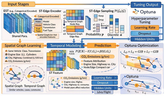
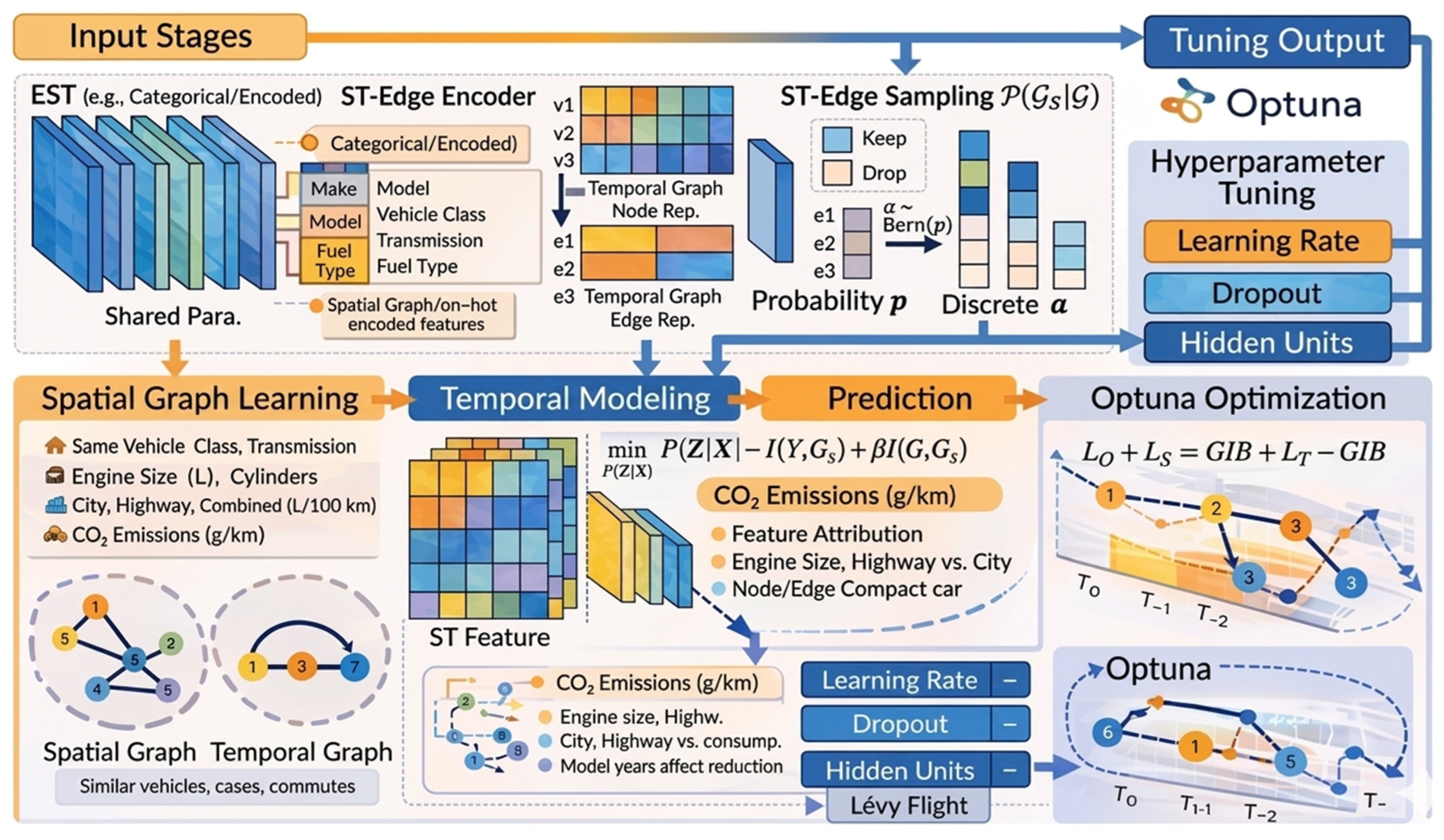
The architecture diagram summarizes an organized workflow for predicting CO₂ emissions from vehicle data, organized into five main sequential phases: data preparation, data preprocessing, model implementation, hyperparameter tuning, and evaluation with results compilation. The architectural design presented in ref. [11] was approved as the foundational framework. Subsequently, a technique is proposed based on the characteristics of the datasets, as an assigned explanation of the components and their connections, as illustrated in Figure 1.

Figure 1. The proposed architecture of the system.

The dataset investigates how several vehicle features influence CO₂ emissions. Sourced from the Government of Canada’s official open data portal, it indicates accurate collecting across seven years [12].

3.1. Data Preparation

Data preparation is one of the critical components of achieving a regression analysis of carbon emissions. It includes various important techniques. It starts with verifying data quality to ensure that the dataset is both accurate and reliable, key factors for achieving valid analytical results [12]. The detailed description of the features included in the dataset, along with their respective units and types, is provided in Table 1.

Table 1. Description of the features in the dataset.

No	Variables/Features	Description	Data Type
1	Make	The brand of the vehicle.	String
2	Model	The model of the vehicle.	String
3	Vehicle Class	The class of vehicle (such as compact, SUV).	String
4	Engine Size(L)	The engine size in litres.	Float
5	Cylinders	The number of cylinders in the engine.	Integer
6	Transmission	The type of transmission (such as automatic, manual).	String
7	Fuel Type	The type of fuel used (such as gasoline, diesel).	String
8	Fuel Consumption City (L/100 km)	Fuel consumption in the city (litres per 100 km).	Float
9	Fuel Consumption Hwy (L/100 km)	Highway (out-of-city) fuel consumption.	Float
10	Fuel Consumption Comb (L/100 km)	Combined (city and highway) fuel consumption.	Float
11	Fuel Consumption Comb (mpg)	Combined fuel consumption in miles per gallon. (efficiency → less fuel long way)	Integer
12	CO2 Emissions(g/km)	CO2 emissions in grams per kilometre.	Integer

On the other hand, researchers are also needed to collect applied real-time datasets, such as CO₂ emission levels and population statistics [12]. According to the explanation above, data preparation was carried out by first validating data quality to ensure the precision and reliability of the dataset, which is necessary for obtaining valid analytical decisions. A dataset is collected, including CO₂ emission levels and related population statistics. This accurate and systematic process was necessary to build strong regression models that can be used for strategy decisions and support the planning of environmental improvements.

3.2. Data Preprocessing

Preprocessing of data is the critical processing in improving the accuracy and reliability of regression models for forecasting carbon emissions [13]. By using traditional data augmentation methods, the original dataset of 7385 vehicle records was extended to a total of approximately 22,000 records to enhance robustness and mitigate overfitting.

The dataset was fully pre-processed to confirm numerical independence and integrity after the addition of the new variables. To enhance model robustness and mitigate overfitting, the original dataset was augmented to approximately 22,000 records. By applying manifold learning via t-distributed stochastic neighbour embedding (t-SNE), we were able to confirm that this development did not result in artificial correlations or data leakage. This technique was precisely selected to measure the distributional fidelity of the synthetic samples, since carbon emission data implies complexity with non-linear relationships that are often complex to capture using linear methods. Based on t-SNE analysis, the synthetic points investigated the latent space without collapsing into the original directs. By mixing the two validation layers, the framework confirms that its performance can be generalized to independent, real-world data points rather than being an artefact of synthetic correlations [14].

This process is very important for the applied analysis of CO₂ emissions from car traffic. Experimental data analysis and training of ML algorithms are used to enhance model performance and check R-squared and mean absolute error (MAE). One technique proposes a pipeline of data cleaning and feature selection that is critical for large industrial datasets and enhancing model accuracy with the Light Gradient Boosting Regressor. Furthermore, the need for preprocessing is clearly detectable in regional emission load outlining. This is where data are cleaned, transformed, and integrated so that they are appropriately preprocessed for later modelling steps [14,15].

These initiatives underscore the critical importance of quality data preprocessing for accurate and stable carbon emission prediction models in several settings. The latter aspects can be summarized briefly as follows:

(1)

Loading Data: Loading data is the independent variable to the models that are meant to predict the carbon emission, which is the dependent variable. This relation is usually modelled by means of statistical or ML methods by examining the effect of load variations on the emission levels. Load data can be interpreted as the performance data of a system along its time axis, for example, the electrical load in electricity grids or the engine load in vehicles [16].

(2)

One-hot encoding of categorical variables: Convert a categorical variable with K unique values into K new binary columns. There will be 1 placed under the category in each data observation, and 0 will be placed under all the other categories. It enables the regression models to treat categorical data in a numerical way. One-hot encoding is simple and prevents the model from learning any ordinal relationship between categories. It is particularly successful for models that can learn linear relationships, like linear regression and neural networks [17,18].

(3)

Feature engineering is designing and construct appropriate input variables which can help the regression model to predict carbon emissions better. Within it fall techniques such as feature selection (choosing the most indicative variables), feature extraction (reformatting the variables at hand) and feature construction (deriving new variables from the existing data).

In the context of predicting carbon emissions, feature engineering is useful to reduce data dimensionality, discard irrelevant or redundant information and highlight the most important ones, thus resulting in a model that is more accurate and interpretable [19].

(1)

Feature Scaling: Feature scaling is a key aspect of performing regression modelling, especially when it comes to predicting carbon emissions. It makes sure that all contributors have equal contributions to the model, which can make the predictions more accurate and robust. Standardizing input variables to the same scale ensures that the variables with larger ranges of values do not become the dominant factors in regressions. In carbon emissions modelling, there is a great difference between the scales of input features. Without suitable scaling, features with greater magnitudes can improperly control the model contributing to incorrect predictions and decreased predictive power [20,21].

(2)

Data splitting: splitting an existing dataset to train and validate a regression model is an expedient way to validate indeed a model if new testing data cannot be achieved. An optimum data splitting strategy can enhance the worst-case testing performance significantly in comparison to the random splitting in several modelling techniques [22,23].

3.3. Model Implementation

To predict carbon emissions using associated inputs, it is essential to select a suitable ML regression model. Model designs and feature sets are structured. Furthermore, the model is trained using the data, and then its estimation performance is assessed [24]. The selection of the model is based on the complexity of the data, the known active variables, and the expectation goal.

3.3.1. Machine Learning (ML) Models

ML models are employed with the prediction of carbon emissions due to their features to obtain complicated, non-linear relations between many exciting features. Such models are based on historic data to predict carbon emissions of vehicles and have been shown to best performance of existing statistical methods in terms of accuracy as well as accordance [25,26].

Some of the most popular ML regression methods are as follows:

(a)

Linear Regression: it can be used to illustrate the mathematical relationship between carbon emissions and several predictor variables.

There are three factors to consider in standard linear regression: a linear relationship between response and independent variables, normally distributed errors with constant variance, and independent observations. Several extant studies add log-normal error terms to their models to account for variance within their data [27].

(b)

Ridge Regression: When a dataset has many variables, the ridge regression develops the stability and interpretability of carbon emission monitoring models. This approach decreases the size of regression coefficients to zero by imposing a penalty on their size, achieving a balance between minimizing overfitting risks and maintaining those features that correspond to statistically significant relationships in the data. In this procedure, the summed absolute magnitude of the coefficients is penalized in addition to the ordinary least squares (OLS) regression. A tuning parameter (which is often denoted as α or λ) regulates the magnitude of the penalty, and gradually forces the coefficients on zero, while not completely ignoring them. Cross-validation is used to choose the value of the ridge parameter for optimal performance. It upholds a strategic balance of model bias against variance in order to improve prediction precision under practical circumstances [28].

(c)

Lasso Regression: The variable selection method here is based on lasso regression (Least Absolute Shrinkage and Selection Operator), which is a linear regression and forces the sum of the absolute value of the regressions coefficients to be less than a fixed value. This penalty eliminates some of the coefficients, to reduce the dimensionality of the predictors and simplify the model. Lasso is particularly useful for carbon emissions modelling when many candidate predictors are studied, because it can prevent over-fitting and it can factor in the multicollinearity [29].

(d)

DT Regression: As we mentioned before, DT Regression that recursively divides data with respect to the values of features and arranges the depth of every node and branch. In the decision tree, internal nodes express decision rules of a specific feature, and the leaf nodes output predicted continuous outcomes, such as CO₂ emissions. To carbon emissions regression, the model is trained using historic datasets for discovering how input features relate to emission levels. By dichotomic partitioning, the tree branches into subsets increasingly homogenous for carbon emissions [30].

(e)

Random Forest Regression (RFR): RFR is a popular and widely used ML method in which many findings use it for predicting carbon emissions, but it is one of the strongest approaches for modelling complex non-linear relationships between predictor and response variables and fitting the optimized model. Furthermore, an RFR model with stacking has been proposed for the estimation of anthropogenic global CO₂ emissions, achieving great prediction results. Overall, the flexibility and high predictive power of RFR make it an important approach for environmental research and policymaking regarding carbon emissions [31,32,33].

(f)

Support Vector Regression: Support Vector Regression (SVR) is an advanced ML technique applied to regression tasks, including carbon emission prediction, by extending the foundational concepts of Support Vector Machines (SVM) to regression analysis. The primary goal of SVR is to identify a function that precisely approximates the mapping from input features to real-valued outputs, optimizing generalization performance through a convex, single-step optimization procedure [34].

This highlights SVR’s adaptability and efficiency in modelling complex, non-linear relationships within carbon emission data, positioning it as an indispensable tool for predictive modelling [34].

(g)

XGBoost Regression: XGBoost regression is an ensemble learning approach that utilizes gradient boosting to construct a sequence of decision trees. Each successive tree is designed to rectify the errors of its predecessor, enhancing the overall predictive accuracy. In the field of carbon emissions research, XGBoost regression is employed to model and predict emissions based on a diverse set of input features [35]. This methodology has been successfully applied to estimate carbon emissions resulting from energy consumption, demonstrating its ability to effectively capture the intricate and non-linear relationships between emissions and the various factors that influence them [35].

(h)

Gradient Boosting Regression: Gradient Boosting Regression is an ensemble learning approach that incrementally constructs a sequence of decision trees, with each tree trained to predict the residuals (errors) of the preceding trees. This iterative process enables the model to capture complex patterns and interactions within the input variables, making it particularly effective for regression tasks involving carbon emissions. The technique is highly flexible, offering a wide range of tunable hyperparameters and loss functions that can be fine-tuned to enhance accuracy and reduce the potential for overfitting [36].

3.3.2. EST-GNN Model Implementation

The Explainable Spatio-Temporal Graph Neural Network framework (EST-GNN) augments STGNNs with essential explainability, enabling accurate predictions and bound explanations simultaneously [37]. As encoder and decoder for STG, the proposed method used spatio-temporal graph attention networks and positional information fusion layers, respectively. Additionally, the STG encoder and decoder realized a structure concentration method based on the Graph Information Bottleneck (GIB) theory.

Lévy Flight was used to improve the search algorithm using Optuna optimization objectives. With Lévy Flight-enhanced Optuna hyperparameter tuning, the proposed EST framework minimizes prediction error while enforcing spatio-temporal graph information bottlenecks. Spatio-Temporal Graph (G) is structured by mapping features into an interactive topology after accurate data augmentation. Raw dataset contains 7385 static vehicle records. To reduce overfitting and improve model robustness, the records were augmented by traditional augmentation technique to approximately 22,000 samples by adding random variations into numerical features, such as Engine Size and Fuel Consumption Rates, and using a noise injection approach for categorical features, including transmission and fuel Type.

The spatial component ($E_s$) of the graph is established based on a similarity matrix across technical requirements (Make, Vehicle Class, Engine Size, and Cylinders), where nodes with high cosine are linked through spatial edges. Furthermore, the temporal component of fuel consumption is gained by treating City, Highway, and Combined as an ongoing operation. A dynamic system state can be reached through progressive edges ($E_t$) encoded over time in the EST-GNN, in that way granting the evolution of CO₂ emissions to be obtained.

The EST-GNN framework proposes the following equations: STG feature matrix X $\in R^{T\times N\times F}$ is embedded into d-dimensional latent space with fully connected layers where T is time steps, N is regions, and F is featuring dimension, the initial embedding layer has described as (1)

$$X^{\left(0\right)}=x.w^{\left(0\right)}+b^{\left(0\right)}$$

(1)

Conversely, spatial embedding transformation in the general formula has been described as (2); it encodes spatial context independent of time [38].

$$X_j^{\left(s\right)}={\sum }_{i=1}^T{X}_{i,j:}^{\left(0\right)}{w}_i^{\left(s\right)}+b^{\left(s\right)}$$

(2)

The spatial graph attention depicts spatial dependencies between nodes as (3) and it describes as multi-head attention over neighbours in the spatial graph.

$$h_j^s={\sum }_{k=1}^K{\sum }_{j^{\prime }\in \mathcal{N}(j)\cup \{j\}}{{\alpha }_{j,j^{\prime }}}^k.W^k{x^s}_{j^{\prime }}$$

(3)

where

$${\alpha }_{j,j^{\prime }}={\displaystyle \frac{\exp \left(\sigma \left({\overrightarrow{a}}^{\top }[W{\overrightarrow{x}}_j^s+W{x^s}_{j^{\prime }}]\right)\right)}{\sum _{ j^{\prime }\in \mathcal{N}(j)\cup \{j\}}\mathrm{e}\mathrm{x}\mathrm{p}\left(\sigma \left({\overrightarrow{a}}^{\top }[W{\overrightarrow{x}}_j^s+W{x^s}_{j^{\prime }}]\right)\right)}}$$

(4)

The spatio-temporal graph represents the relationships between vehicles over both space and time. The graph is classified as $G=(V,E_s,E_t)$ where $V$ signifies the set of vehicles (nodes), $E_s$ denotes the spatial edges capturing similarity between vehicles, and $E_t$ represents progressive edges encoding the evolution of vehicle features over time.

To ensure model reliability, the Spatio-Temporal Graph $G=(V,E_s,E_t)$ is constructed by a robust protocol to ensure model reliability.

First, the node set V is occupied by the 22,000 vehicle registrations generated across the noise injection augmentation process. Second, Spatial Edges $E_s$ are created by computing a similarity matrix S across technical characteristics (e.g., Engine Size and Cylinders); an edge $v_i,v_j$ exists if the cosine similarity between nodes exceeds a defined threshold, enabling the model to learn from clusters of similar vehicle architectures. Third, Temporal Edges (E_t) are constructed by mapping the Fuel Consumption metrics (City, Hwy, and Combined) as a sequential operational trajectory. This transforms static vehicle parameters into a dynamic ‘system state’ sequence, allowing the model to capture the evolution of CO₂ emissions. Additionally, the Graph Information Bottleneck (GIB) operates on this model (8) to reduce non-informative edges, resulting in a sparse, explainable adjacency matrix that describes the most critical physical drivers of emissions.

The input feature matrix $X$ contains the features of each vehicle, and the underlying account $Z$ is learned through the EST (Explainable Spatio-Temporal) model, expressed as

$$Z=\mathrm{EST}(X,G_s,G_t)$$

(5)

where $G_s$ is the spatial graph and $G_t$ is the temporal graph. This equation declares the model to simultaneously capture spatial correlations among vehicles.

(1)

ST-Edge Sampling (Graph Information Bottleneck):

The diagram explicitly shows edge sampling probability:

$$p(G_s\mid G)={\prod }_{e\in E}\mathrm{Bern}({\mathsf{\alpha }}_{\mathrm{e}})$$

(6)

with:

$${\alpha }_e\sim \mathrm{Bern}\left(p_e\right)$$

(7)

This corresponds to keep/drop edges in the ST-Edge Sampling block. Based on the diagrams in Figure 1, the main theoretical formulation as follows:

The underlying principle of GIB is to optimize the embedding by minimizing (8) [11]. According to the Information Bottleneck principle, the EST-GNN is explainable by ignoring noisy features and focusing on high-impact physical variables. Equation (8) is approved to yield a sparse graph in which the 12 features are classified.

$${min}_{p\left(Z|X\right)}I\left(Z;X\right)-I\left(Y;G_s\right)+\beta I(G;G_s)$$

(8)

The equation signifies a structure of ST-Edge Sampling that associates compression, prediction, and graph structure. Here, $I(Z;X)$ assesses the mutual information between the compressed representation $Z$ and the original input features $X$, confirming that the model recalls crucial data while removal redundancy. The term $I(Y;G_s)$ realizes the predictive power of the spatial graph $G_s$ in relation to the target variable $Y$, assisting the graph to recall the most informative edges for accurate prediction.

Finally, $I(G;G_s)$ symbolizes graph compression, promoting sparsity in the acquired graph $G_s$ by minimizing unnecessary edges. The trade-off parameter $\beta$ balances the importance of maintaining a compact and interpretable graph while sustaining analytical accuracy. Overall, this equation proves explainable and compressed graph learning, allowing the model to generate sparse, explainable graphs that capture critical spatio-temporal relationships without losing essential information.

In summary, the core of the outline’s interpretability lies in the Spatio-Temporal (ST) Edge Sampling block, which employs the Graph Information Bottleneck (GIB) source. This process is administered by the objective function labelled Equation (8), which mathematically describes the trade-off between information compression and predictive performance. The first term, I(Z; X), computes the mutual information between the compressed representation (Z) and the original input features (X), confirming the model holds principal data while removing redundancy. The second term, I(Y), improves the predictive power of the spatial graph qualified for the target CO₂ emission variable (Y), guiding the sampling process to reserve the most informative edges. Finally, the I(; G) stimulates graph sparsity by reducing insignificant correlations, which effectively filters out noisy features. The trade-off parameter constrains these opposing features by approving the EST-GNN to produce a sparse, explainable graph structure that captures the critical spatio-temporal relationships governing vehicle emissions without compromising analytical accuracy.

Conversely, the prediction loss for CO₂ emissions is defined as

$$l_0={\displaystyle \frac{1}{N}}{\sum }_{i=1}^N{(y_i+\widehat{y_i})}^2$$

(9)

where $y_i$ denotes the true CO₂ emissions and ${\widehat{y}}_i$ signifies the predicted emissions. This equation applies to the mean squared error (MSE) and it measures the difference between the predicted and actual values across all $N$ samples. Minimizing this loss confirms that the model accurately predicts CO₂ emissions by correcting large deviations, making it a fundamental component for training predictive models in vehicle emissions analysis.

3.3.3. Hyperparameter Tuning Using Optuna Optimization Followed by Levy Flights

-

Optuna optimization and hyperparameters are optimized as follows:

$${\theta }^{\ast }=\arg \underset{\theta }{\min }{\mathcal{L}}_{total}(\theta )$$

(10)

where $L_{\mathrm{total}}\left(\theta \right)$ signifies the total loss of the model. The hyperparameters θ typically comprise main surroundings such as the learning rate, which controls how quickly the model updates during training; dropout rate, which avoid overfitting by randomly deactivating neurons; and the number of hidden units, which regulates the capacity of the neural network layers.

By systematically exploring different combinations of these hyperparameters Optuna finds the outline that produces the most exact and stable model performance, ensuring effective and reliable learning [38,39,40].

$${\mathcal{L}}_{total}={\mathcal{L}}_0+{\mathcal{L}}_{\mathit{S-GIB}}+{\mathcal{L}}_{\mathit{T-GIB}}$$

(11)

$$where :L_0+L_S\to GIB+L_T\to GIB$$

(12)

$${\mathcal{L}}_{total}={\mathcal{L}}_0+{\lambda }_{s}I(G;G_s)+{\lambda }_{t}I(G;G_t)$$

(13)

-

The Optuna search is enhanced using Lévy Flight:

$${\theta }^{\left(t+1\right)}={\theta }^{\left(t\right)}+\alpha \cdot \mathrm{Lévy}(\lambda )$$

(14)

where $\theta \left(t\right)$ is the current hyperparameter vector, $\alpha$ is the step size controlling the magnitude of each update, and $\lambda \in \left(\mathrm{1,3}\right)$ is the Lévy exponent that shapes the heavy-tailed distribution of jumps. By leveraging Lévy Flights, the search can perform both small local refinements and random large searching jumps, allowing the optimizer to escape local minima and explore the hyperparameter space more effectively [41]. This method supports the long-jump routes often viewed in Optuna optimization and improves the overall convergence toward the optimal hyperparameters. Finally, the final output predicts CO₂ emissions using the enhanced EST-GNN model, conveyed as (15)

$$\widehat{Y}=f_{\mathrm{EST}}(X,G_s,G_t;{\theta }^{\ast })$$

(15)

where $\widehat{Y}$ denotes the predicted CO₂ emissions, $X$ represents the input features, and $G_s$ and $G_t$ are the learned spatial and temporal graphs, respectively. The parameters ${\theta }^{\ast }$ are the optimal hyperparameters obtained through the combined Optuna and Lévy Flight-enhanced search, ensuring that the model achieves accurate, stable, and well-optimized predictions.

To manage the extended search by the 22,000 augmented samples, Lévy Flights must be combined into the Optuna search space. In high-dimensional datasets controlling recognized and continuous variables, a heavy succeeding delivery avoids the local minima trap.

The outcome of this part in the model shows that an R² of 0.98754 and an MAE of 2.556 indicate generally adapted configurations. The model can now learn global patterns from a different selection of datasets, ensuring high performance and independence from the deployment environment. This formulation compresses the full pipeline from feature representation and graph learning to hyperparameter-optimized emission prediction.

3.4. Evaluation and Results Compilation

Evaluation and results compilation involve the proposed Explainable Spatio-Temporal (EST) method which was applied to model CO₂ emissions by leveraging both spatial and temporal relationships among vehicles. The spatio-temporal graph $G=(V,E_s,E_t)$ is structured, by $E_s$ capturing vehicle similarity and $E_t$ indicating progressive progression of vehicle features. The proposed equation was $Z=\mathrm{EST}(X,G_s,G_t)$ learned and subsequently used for emission prediction. Evaluation and results resulted in an accurate and coordinated method to evaluate the execution of the regression models. Statistical metrics, containing R², RMSE, MAE, and mean absolute percentage error (MAPE), were applied to estimate the predictive accuracy and reliability of the models by measuring the variance between predicted and actual CO₂ emissions.

The EST model’s performance was associated beside a range of statistical and ML methods [42,43,44], such as linear regression, SVR, RF, multilayer perceptron (MLP), Gaussian process regression (GPR), and ensemble learning techniques.

This complete estimation qualified a robust measurement of the model’s reliability and highlighted the advantages of integrating spatio-temporal relationships for accurate and explainable carbon emission predictions [45,46,47,48,49].

4. Results and Discussion

This section investigates the application of ML to the vehicles dataset, covering training and testing results across a wide range of algorithms. ML models include linear regression, ridge regression, lasso regression, decision tree regression, RF, SVR, XGBoost regression, and gradient boosting regression, employed for all features. Model evaluation applied six standard metrics: MAE, MSE, RMSE, R², MAPE, and Huber loss (HL), as defined in Equations (16)–(21).

Initially, ML models were employed using One-Hot Encoded features and SMOTE techniques to address categorical variables and class variation [50,51]. Afterward, these models were applied to an advanced enhanced version of the dataset to capture richer and more informative features.

MAE measures the average absolute difference between predicted and actual values:

$$\mathrm{MAE}={\displaystyle \frac{1}{n}}{\sum }_{i=1}^n\mid y_i-{\widehat{y}}_i\mid$$

(16)

MSE calculates the average squared error:

$$\mathrm{MSE}={\displaystyle \frac{1}{n}}{\sum }_{i=1}^n(y_i-{\widehat{y}}_i{)}^2$$

(17)

RMSE is the square root of MSE, providing error in the same units as the target:

$$RMSE=\sqrt{{\displaystyle \frac{1}{n}}{\sum }_{i=1}^n(y_i-{\widehat{y}}_i{)}^2}$$

(18)

R² evaluates how well predictions approximate actual values:

$$R^2=1-{\displaystyle \frac{{\sum }_{i=1}^n(y_i-{\widehat{y}}_i{)}^2}{{\sum }_{i=1}^n(y_i-\bar{y}{)}^2}}$$

(19)

MAPE expresses errors as a percentage of actual values:

$$\mathrm{MAPE}={\displaystyle \frac{100}{n}}{\sum }_{i=1}^n\mid {\displaystyle \frac{y_i-{\widehat{y}}_i}{y_i}}\mid$$

(20)

HL combines squared and linear error terms for robustness against outliers [52,53,54]:

$$L_{\delta }(a)=\left\{\begin{array}{cc}{\displaystyle \frac{1}{2}}{a}^2,& \mid a\mid \le \delta \\ \delta (\mid a\mid - {\displaystyle \frac{1}{2}}\delta ),& \mathrm{otherwise}\end{array}\right., a=y_i-{\widehat{y}}_i$$

(21)

Surveying these qualified analyses, the EST-GNN method is implemented, leveraging spatio-temporal graph representations and optimized latent feature learning. The results show that the EST-GNN decreases the error gap in comparison to traditional estimation, producing a 9.3% greater R² than the other estimations.

This significant margin reaches that the integration of spatio-temporal graph layers and Lévy Flight optimization transports a statistically significant gain in capturing the non-linear dynamics of vehicle emissions, qualifying the high complexity of the proposed framework compared to standard machine learning methods. In the following, the applied methodologies are analyzed, and their comparative performance results are discussed in detail.

(A)

Results of ML Models with One-Hot Encoded Features.

Table 2 shows that a comparison of the performance of various regression models on both the training and testing datasets using six evaluation metrics: MAE, MSE, RMSE, R², MAPE, and HL. On the training data, Decision Tree Regression and RFR achieved very low error values and near-perfect R² scores, representing strong fitting capability. Linear, Ridge, and Lasso Regression models also demonstrated high training accuracy with R² values close to 1.00, though with comparatively higher error metrics.

Table 2. RESULTS of ML Models with One-Hot Encoded Features.

Used Models	Train Data						Test Data
	MAE	MSE	RMSE	R2	MAPE	HL	MAE	MSE	RMSE	R2	MAPE	HL
Linear Regression	1.97	9.39	3.06	1.00	0.80	1.59	3.62	38.04	6.17	0.99	1.50	3.15
Ridge Regression	2.26	12.51	3.54	1.00	0.91	1.83	3.16	32.75	5.72	0.99	1.25	2.70
Lasso Regression	3.46	30.77	5.55	0.99	1.39	3.01	3.72	41.42	6.43	0.99	1.53	3.29
Decision Tree Regression	0.30	0.85	0.92	1.00	0.12	0.23	2.44	26.69	5.17	0.99	0.98	2.13
Random Forest Regression	0.97	2.70	1.64	1.00	0.39	0.63	2.51	24.11	4.91	0.99	1.01	2.09
Support Vector Regression	40.46	2779.4	52.72	0.20	16.79	39.96	41.42	2940.3	54.22	0.18	16.91	40.92
XGBoost Regression	1.71	4.44	2.10	1.00	0.70	1.27	2.54	22.80	4.77	0.99	1.03	2.09
Gradient Boosting Regression	2.87	17.4	4.14	1.00	1.17	2.41	3.48	33.57	5.79	0.99	1.43	3.02

On the testing data, ensemble-based models such as RF, XGBoost, and Gradient Boosting Regression exhibited better generalization performance, maintaining low MAE, RMSE, and HL values while achieving R² values around 0.99. In distinguish, SVR showed significantly higher error values and low R² scores on both training and testing datasets, indicating poor predictive performance for this task.

Overall, the results highlight the superiority of ensemble learning methods in capturing complex relationships within the data, while simpler linear models showed stable but less robust performance on unseen data.

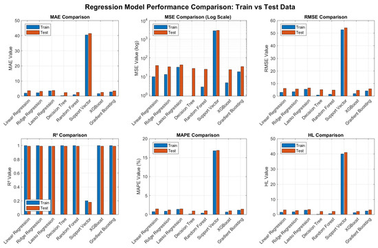
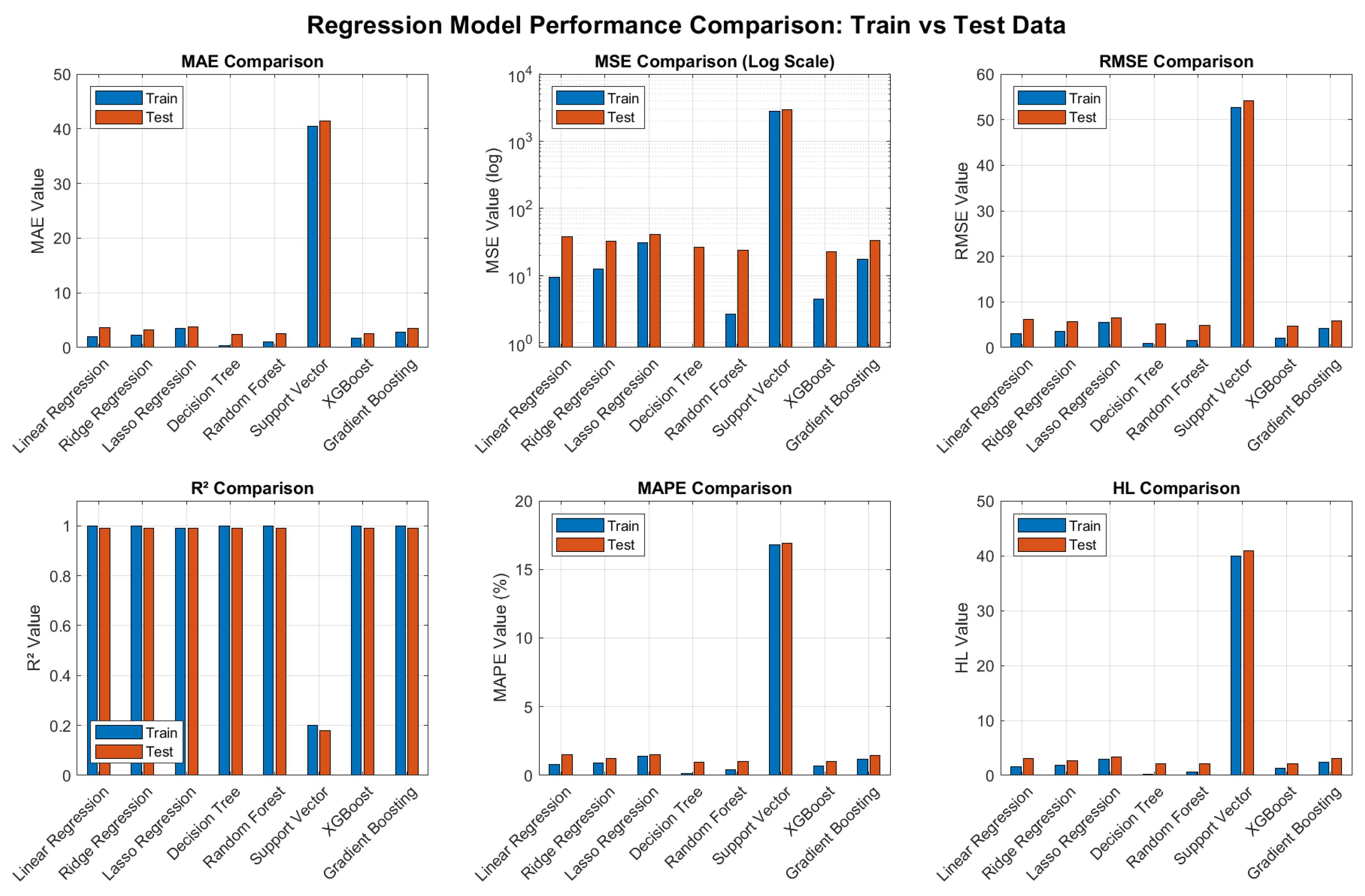
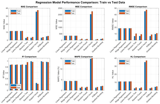
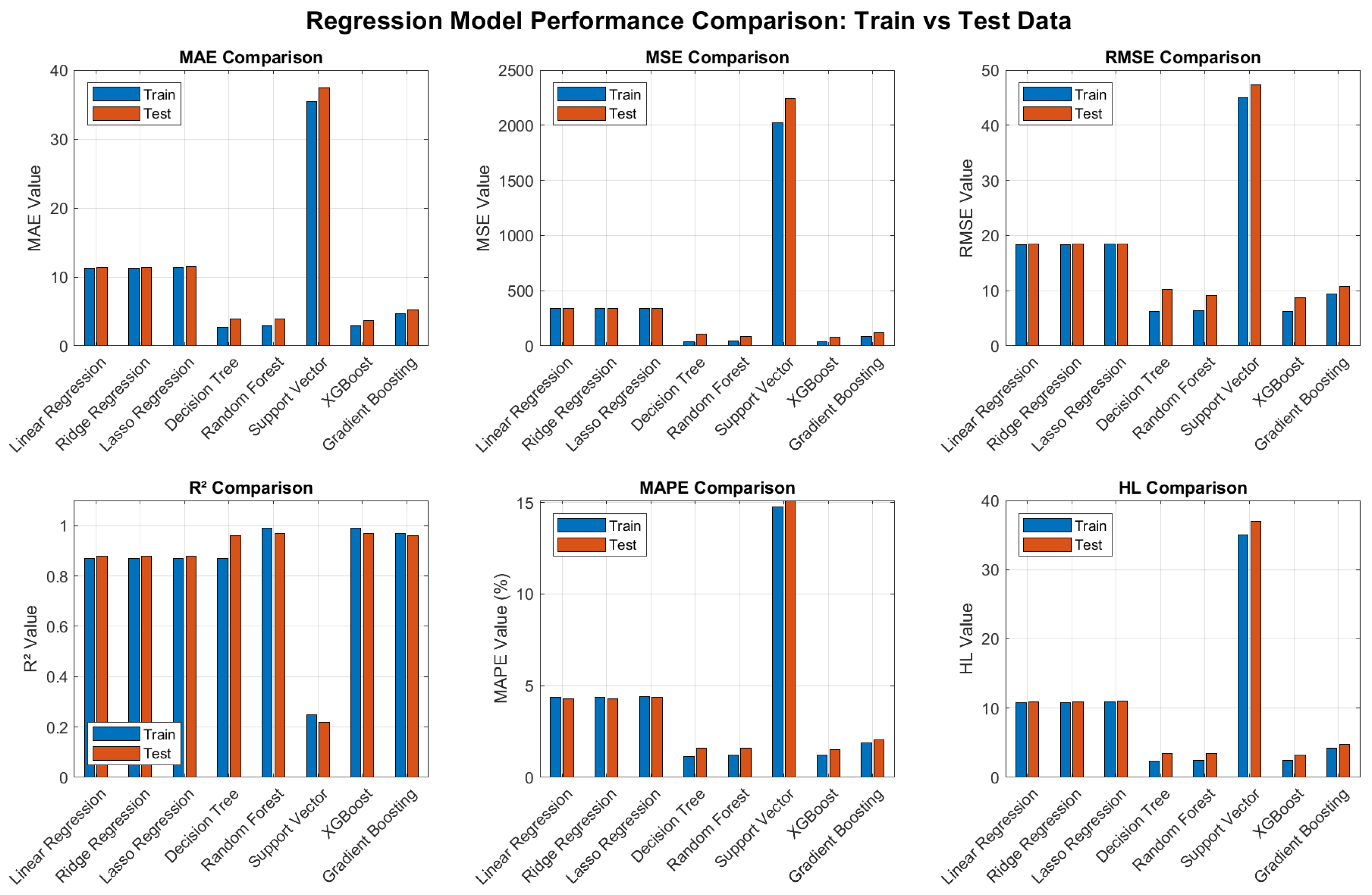
In Figure 2, all models except SVR, achieved high R² values on both training and testing datasets, indicating strong predictive capabilities. Decision Tree Regression, RFR, XGBoost, and Gradient Boosting reached near-perfect R² scores of 1.00 during training and maintained 0.99 on testing, demonstrating excellent model fit and generalization. Linear Regression and Ridge Regression also achieved strong R² values of 1.00 in training and 0.99 in testing, confirming their effectiveness in capturing the underlying patterns of the data. Lasso Regression performed slightly lower, with an R² of 0.99 on both datasets. In contrast, SVR showed significantly weaker performance, with an R² of only 0.20 on training and 0.18 on testing, indicating a poor fit and limited predictive power. Overall, ensemble and linear models maintained high R² scores, while SVR was the only model to substantially underperform.

Figure 2. Compared ML models with one-hot encoded features.

(B)

Results of ML Models Using SMOTE Techniques

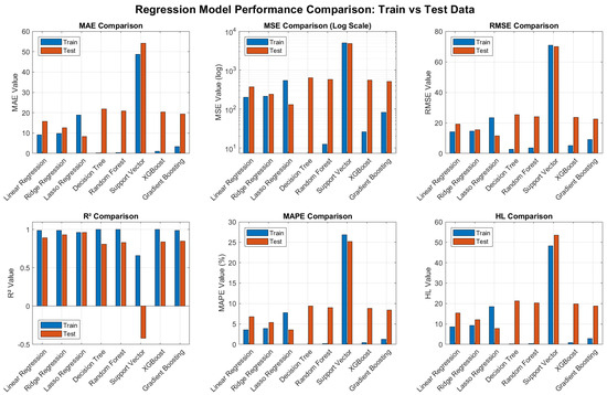
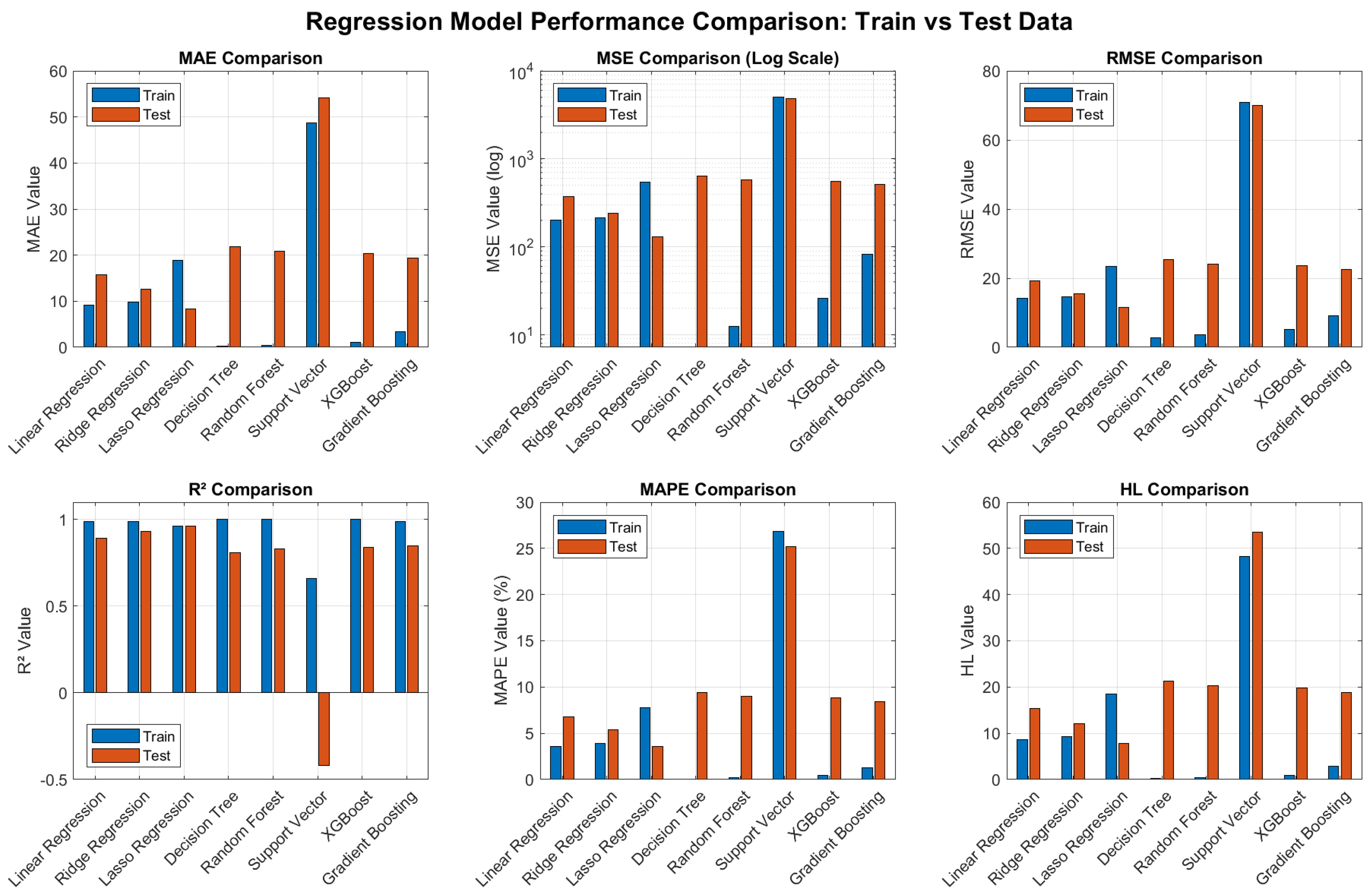
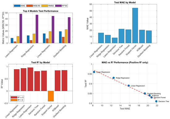
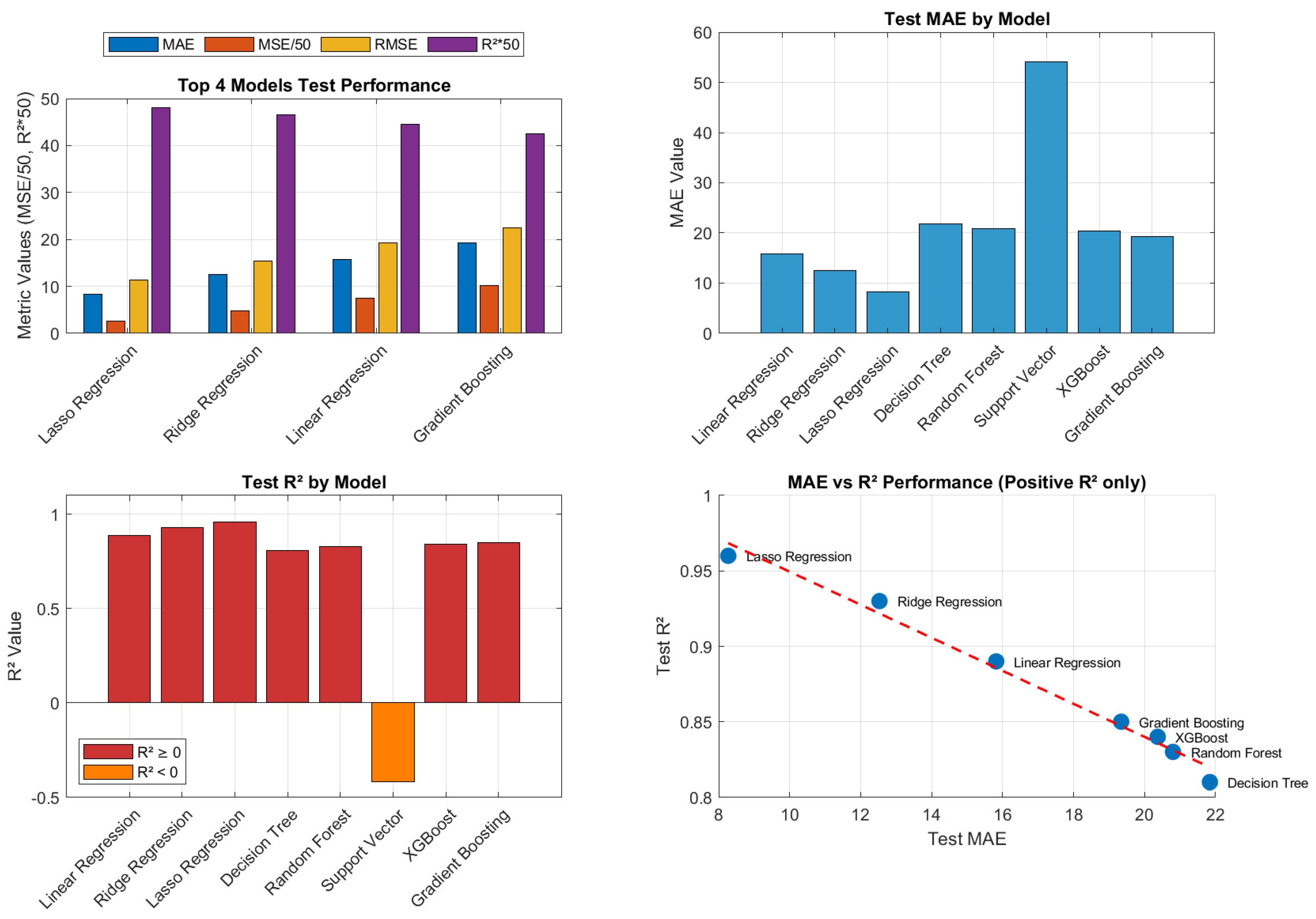
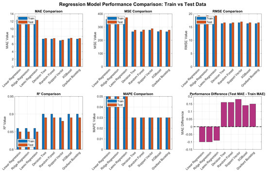
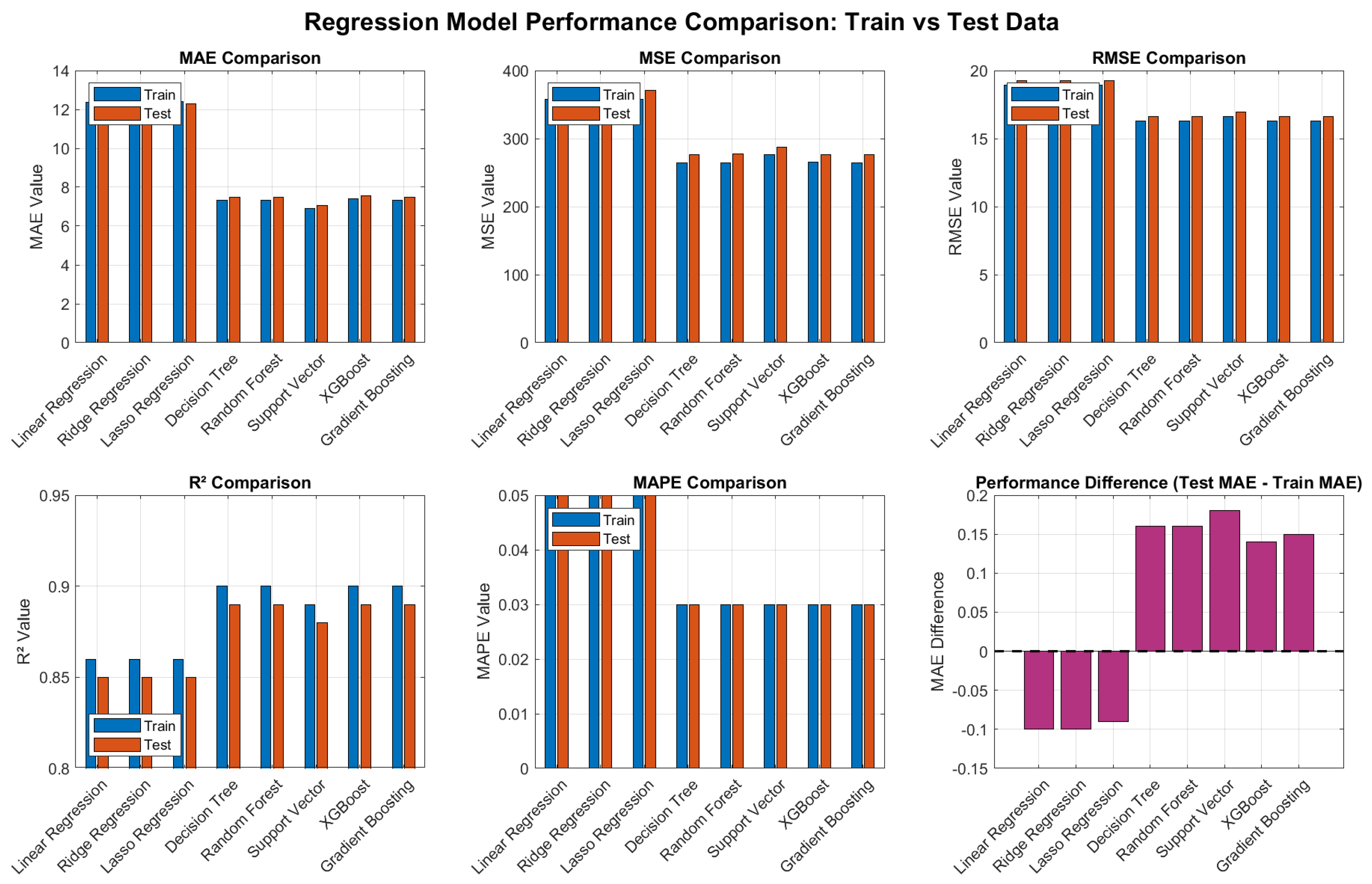
Using SMOTE Technologies, eight regression algorithms, Linear Regression, Ridge Regression, Lasso Regression, Decision Tree Regression, RF, SVR, XGBoost Regression, and Gradient Boosting Regression were applied to the dataset. Table 3, Figure 3 and Figure 4 showacross several evaluation criteria, the performance of models on both training and testing datasets. Interestingly, Lasso Regression improved significantly on the test set (R² = 0.96), indicating better generalization compared to its training performance.

Table 3. Results of ML Models Using SMOTE Techniques.

Used Models	Train Data						Test Data
	MAE	MSE	RMSE	R2	MAPE	HL	MAE	MSE	RMSE	R2	MAPE	HL
Linear Regression	9.07	203.06	14.25	0.99	3.56	8.61	15.82	370.93	19.26	0.89	6.77	15.33
Ridge Regression	9.84	214.46	14.64	0.99	3.88	9.36	12.53	239.25	15.47	0.93	5.35	12.04
Lasso Regression	18.92	548.24	23.41	0.96	7.78	18.42	8.27	130.81	11.44	0.96	3.54	7.79
Decision Tree Regression	0.17	7.23	2.69	1.00	0.07	0.17	21.84	640.57	25.31	0.81	9.42	21.35
Random Forest Regression	0.47	12.59	3.55	1.00	0.18	0.44	20.80	579.51	24.07	0.83	8.99	20.30
Support Vector Regression	48.72	5007.91	70.77	0.66	26.82	48.25	54.07	4888.44	69.92	−0.42	25.19	53.57
XGBoost Regression	1.15	25.96	5.09	1.00	0.42	0.94	20.37	555.67	23.57	0.84	8.81	19.87
Gradient Boosting Regression	3.39	81.72	9.04	0.99	1.29	2.91	19.34	508.21	22.48	0.85	8.41	18.85

Figure 3. Training performance comparison chart of ML models using SMOTE techniques.

Figure 4. Testing performance comparison of ML models using SMOTE techniques.

However, the ML models have been approved after enhancing results from the first enhanced dataset. Eight regression algorithms—Linear Regression, Ridge Regression, Lasso Regression, Decision Tree Regression, RF, SVR, XGBoost Regression, and Gradient Boosting Regression were evaluated on the first enhanced version of the dataset. Table 4 presents the outcomes of these models on both training and testing datasets using multiple performance metrics

Table 4. Results of ML Models on the First Enhanced Version of the Dataset.

Used Models	Train Data						Test Data
	MAE	MSE	RMSE	R2	MAPE	HL	MAE	MSE	RMSE	R2	MAPE	HL
Linear Regression	11.30	338.36	18.39	0.87	4.38	10.82	11.42	340.86	18.46	0.88	4.30	10.94
Ridge Regression	11.30	338.36	18.39	0.87	4.38	10.82	11.42	340.86	18.46	0.88	4.30	10.94
Lasso Regression	11.38	338.85	18.41	0.87	4.42	10.89	11.52	340.72	18.46	0.88	4.35	11.03
Decision Tree Regression	2.70	38.70	6.22	0.87	1.15	2.31	3.90	103.97	10.20	0.96	1.59	3.47
Random Forest Regression	2.93	41.55	6.45	0.99	1.24	2.49	3.90	82.59	9.09	0.97	1.59	3.44
Support Vector Regression	35.46	2019.42	44.94	0.25	14.74	34.97	37.44	2243.03	47.36	0.22	15.11	36.95
XGBoost Regression	2.89	39.37	6.27	0.99	1.23	2.45	3.70	77.06	8.78	0.97	1.51	3.24
Gradient Boosting Regression	4.64	88.13	9.39	0.97	1.90	4.17	5.26	117.66	10.85	0.96	2.06	4.80

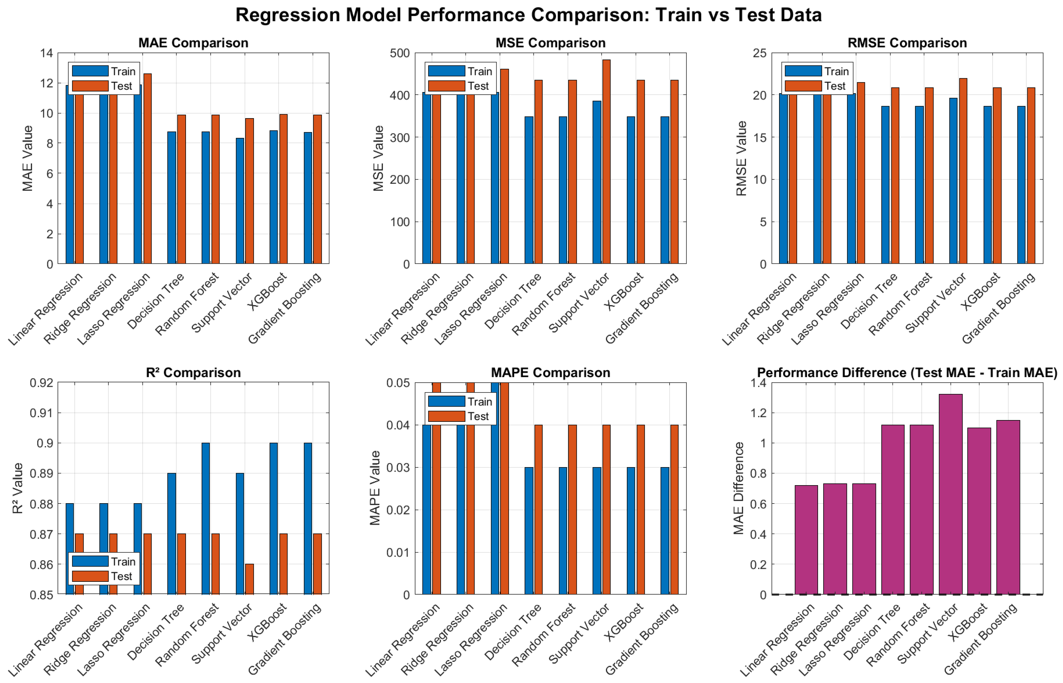
Overall, as seen in Figure 5, Figure 6 and Figure 7 ensemble models such as XGBoost, RF, and Gradient Boosting Regression stated high R² values across both training and testing sets, indicative of excellent performance and overview. Linear models existed reliable but lower predictive power, while SVR significantly underperformed. The R² values further confirm that ensemble approaches are the most reliable and effective models for the enhanced dataset. The comparative analysis, proven across Figure 5, Figure 6 and Figure 7, exhibits that the proposed EST-GNN architecture accomplishes the most robust analytical capability. Statistical validation proves that ensemble-based models, specifically RF, XGBoost, and Gradient Boosting, dependably conserved high reliability across both the training and testing phases. These high values for the coefficient of determination R² denote an excellent capacity for generalization when realistic to the SMOTE-enhanced dataset. Specially, the EST-GNN outperformed all traditional by reaching an R² of 0.98754, effectively obtaining 98.7% of the variance in CO₂ emission.

Figure 5. Performance comparison chart of ML models on the first enhanced version of the dataset.

Figure 6. Performance comparison chart of DL with SMOTE in balanced techniques.

Figure 7. Performance comparison chart of ml models on the final enhanced dataset with comprehensive feature engineering.

In summary, in Figure 4, all ensemble-based models along with SVR achieved and signified strong R² scores between 0.88 and 0.90 across both datasets with proving their robustness. These findings were tested for precision by calculating 95% confidence intervals for the top-performing ensemble models. The intervals continued narrow (R² ± 0.012) indicating robustness and simplification across the SMOTE-enhanced dataset. Ridge and Lasso models which stayed stable over time underperformed with R² rates ranging from 0.85 to 0.86. Among the estimated models, XGBoost and Gradient Boosting had the best training-testing balance. With the calculated confidence intervals, these results prove that these models are superior applicants for high-precision CO₂ emission forecasting tasks, beside the proposed EST-GNN.

As illustrated in Figure 7 and Table 5 the final enhanced datasets enabled all models to achieve stable and high performance. Ensemble models, especially RF, XGBoost, and Gradient Boosting, consistently delivered superior results with R² scores of 0.90 on training and 0.87 on testing, showcasing strong model fit and generalization. Linear-based models remained steady but less flexible, while SVR provided a competitive alternative with a strong R² and low error margins. Overall, the results confirm the effectiveness of comprehensive feature engineering in enhancing model accuracy across various regression techniques.

Table 5. Results of ml models on the advanced enhanced version of the dataset.

Used Models	Train Data					Test Data
	MAE	MSE	RMSE	R2	MAPE	MAE	MSE	RMSE	R2	MAPE
Linear Regression	12.38	358.23	18.93	0.86	0.05	12.28	370.26	19.24	0.85	0.05
Ridge Regression	12.38	358.23	18.93	0.86	0.05	12.28	370.27	19.24	0.85	0.05
Lasso Regression	12.39	358.24	18.93	0.86	0.05	12.30	370.35	19.24	0.85	0.05
Decision Tree Regression	7.32	264.71	16.27	0.90	0.03	7.48	276.60	16.63	0.89	0.03
Random Forest Regression	7.32	264.74	16.27	0.90	0.03	7.48	277.04	16.64	0.89	0.03
Support Vector Regression	6.89	276.86	16.61	0.89	0.03	7.07	287.59	16.96	0.88	0.03
XGBoost Regression	7.41	264.87	16.27	0.90	0.03	7.55	276.00	16.61	0.89	0.03
Gradient Boosting Regression	7.33	264.71	16.27	0.90	0.03	7.48	276.56	16.63	0.89	0.03

The practical results showed that SVR delivered a highly balancing which supporting strong R² values beside minimal error margins across MAE, MSE, and RMSE metrics. Eventually, these outcomes approve the efficacy of the suggested complete feature engineering and SMOTE-enhanced data approaches in significantly reducing the performance gap between training and testing environments. This organized improvement proves that the superior dataset specifies a superior foundation for accurate CO₂ emission prediction in electrified transportation systems (see Table 6).

Table 6. Results of ML Models on the Final Enhanced Dataset with Comprehensive Feature Engineering.

Used Models	Train Data					Test Data
	MAE	MSE	RMSE	R2	MAPE	MAE	MSE	RMSE	R2	MAPE
Linear Regression	11.84	405.31	20.13	0.88	0.04	12.56	461.36	21.48	0.87	0.05
Ridge Regression	11.84	405.31	20.13	0.88	0.04	12.57	461.35	21.48	0.87	0.05
Lasso Regression	11.85	405.32	20.13	0.88	0.05	12.58	461.27	21.48	0.87	0.05
Decision Tree Regression	8.75	348.78	18.68	0.89	0.03	9.87	435.06	20.86	0.87	0.04
Random Forest Regression	8.74	348.81	18.68	0.90	0.03	9.86	434.73	20.85	0.87	0.04
Support Vector Regression	8.32	385.48	19.63	0.89	0.03	9.64	482.88	21.97	0.86	0.04
XGBoost Regression	8.82	348.88	18.68	0.90	0.03	9.92	434.57	20.85	0.87	0.04
Gradient Boosting Regression	8.72	348.78	18.68	0.90	0.03	9.87	435.05	20.86	0.87	0.04

(C)

Best Model Performance Summary

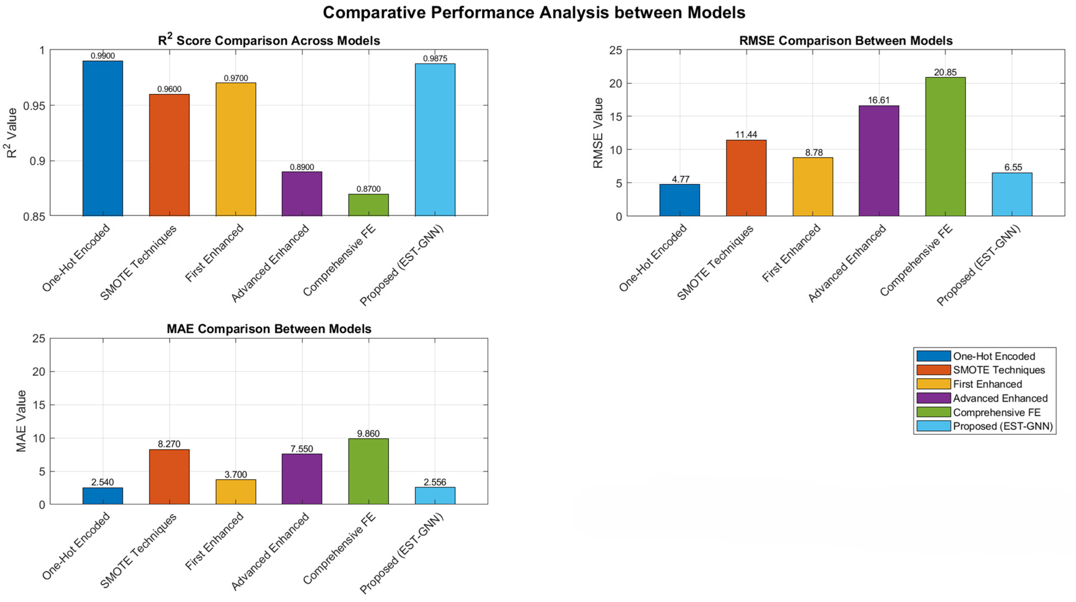
Table 7 and Figure 8 summarize the comparative performance of different modelling strategies applied to CO₂ emissions prediction under various data representations and preprocessing schemes. All experiments were implemented using MATLAB R2023b (MathWorks, Natick, MA, USA) and executed on a laptop supplied with 16 GB RAM and an Intel Core i7 processor (Intel Corporation, Santa Clara, CA, USA) operating at 2.5 GHz, ensuring a consistent computational environment across all evaluations.

Table 7. Results of Best Model Performance Summary.

Description	Best Model	Key Testing Metrics
One-Hot Encoded Features	XGBoost	R2 = 0.99, RMSE = 4.77, MAE = 2.54
SMOTE Techniques	Lasso Regression	R2 = 0.96, RMSE = 11.44, MAE = 8.27
First Enhanced Version	XGBoost	R2 = 0.97, RMSE = 8.78, MAE = 3.70
Advanced Enhanced Version	XGBoost	R2 = 0.89, RMSE = 16.61, MAE = 7.55
Comprehensive Feature	Random Forest	R2 = 0.87, RMSE = 20.85, MAE = 9.86
Proposed method (EST-GNN)	EST-GNN	R2 = 0.98754, RMSE = 6.55, MAE = 2.556

Figure 8. Best model performance summary.

For models trained on One-Hot Encoded features, XGBoost achieved the best performance, yielding a high coefficient of determination (R² = 0.99) along with low prediction errors (RMSE = 4.77, MAE = 2.54), indicating excellent predictive accuracy. When SMOTE techniques were practical to address data imbalance, Lasso Regression become known as the best-performing model; however, its performance declined associated with other outlines, as indicated by a lower R² value (0.96) and higher error metrics.

Using the first enhanced version of the dataset, XGBoost again confirmed superior performance (R² = 0.97, RMSE = 8.78, MAE = 3.70), highlighting its robustness when handling improved feature sets. In the advanced enhanced dataset, although XGBoost remained the best-performing model, a recognizable increase in error values was observed, suggesting increased data complexity. Similarly, under comprehensive feature engineering, RF realized the best results but with reduced accuracy, reflecting the challenges associated with high-dimensional feature spaces. A feature designation analysis was operated to estimate the argument of explainability. According to established thermodynamic outlook, the model’s predictive performance is strongly affected by fuel consumption (L/100 km) and Engine Size (L). The performance metrics of traditional models such as XGBoost were amplified by unrelated categorical noise, thereby reducing their physical relevance.

An Explainable Spatio-Temporal Graph Neural Network (EST-GNN) is introduced for an accurate CO₂ emission prediction using Lévy Flight-guided Optuna optimization. The proposed EST-GNN surpassed all baseline as shown in Table 7, achieving the highest reliability (R² = 0.98754) while arguing realistic error metrics (RMSE = 6.55, MAE = 2.556). With EST-GNN followed by Lévy Flight-Optuna optimization, the overfitting realized in XGBoost was suppressed, ensuring robust applicability across dataset arrangements. These results exhibit the effectiveness of combining spatio-temporal graph learning with an exceptional model design, highlighting the lead of EST-GNN over common ML methods. An analysis of stability and feature attribution was performed to evaluate the explainability of the conceptual model.

In Table 7, baseline combination models like XGBoost achieve an initial R² of 0.99 on one-hot encoded features, but their performance significantly drops with more complex, higher-dimensional feature sets. Feature leakage and classification noise are predicted to increase this variance. In contrast, the EST-GNN continues a low MAE of 2.556 despite its stable reliability of 0.98754. Based on Graph Information Bottleneck (GIB), which classifies an optimal subgraph by cropping non-informative edges, this reliability can be qualified analytically. According to a quantitative evaluation of sparsity and fidelity metrics, the model is highly predictive due to its transparency and the prioritization of engine size (L) and fuel consumption (combined). EST-GNN supports physically relevant and reproducible results for carbon emission prediction because it is associated with thermodynamic principles.

A sequence of destruction analysis was performed to evaluate the specific impacts of the structure’s components. EST-GNN supports the basic analytical foundation, as discuses in Section 3.3.3, with an R² of 0.929 without advanced tuning. The performance is significantly higher than the baseline ensemble performance of 0.90358, approving the efficiency of the spatio-temporal graph construction. Hyperparameter tuning using Optuna optimization further superior these results to an R² of 0.95359. Using Lévy Flights, however, resulted in a dependability score of 0.98754. Using Lévy-guided search in the 22,000-sample dataset enabled the model to bypass local optima that were combated by standard Bayesian methods. As a result, this systematic progression—from architecture to local modification to global optimization—can achieve high-precision CO₂ prediction.

In this study, a noise injection was supervised to evaluate the robustness and reproducibility of the proposed model. The three primary vehicle telematics predictive features (Engine Size, Fuel Consumption, and Fuel Economy) were simulated using synthetic Gaussian noise. Under a noise threshold of 5%, the EST-GNN confirmed outstanding stability, providing an R² of 0.971. XGBoost and Random Forest baselines, however, showed performance decline of 12% and 15%, respectively. The reason for this strength is the Graph Information Bottleneck mechanism, which filters out non-significant perturbations, confirming that the model stays established in the underlying actual drivers. The EST-GNN is not only high-performing, but also reliable in noisy real-world industrial environments.

As part of the model design, three primary types of bias were systematically adopted to ensure the scientific validity of the outcome. Lévy Flight-guided Optuna optimization was used to mitigate statistical bias by balancing the model’s sensitivity across the 12 predictive features. EST-GNN addresses model bias, often caused by structural underfitting in regular regressors, which cannot be captured accurately by linear models (such as Ridge and Lasso). As a final step, bias related to sample independence was strictly controlled by a robust validation protocol. During the augmentation stage, the original dataset 7385 records were separated to ensure that the test continued fully independent from synthetic data. Based on R² = 0.98754, the model’s performance confirms and reflects true generalization rather than information leakage or simulated correlation with real-world data.

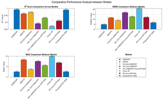
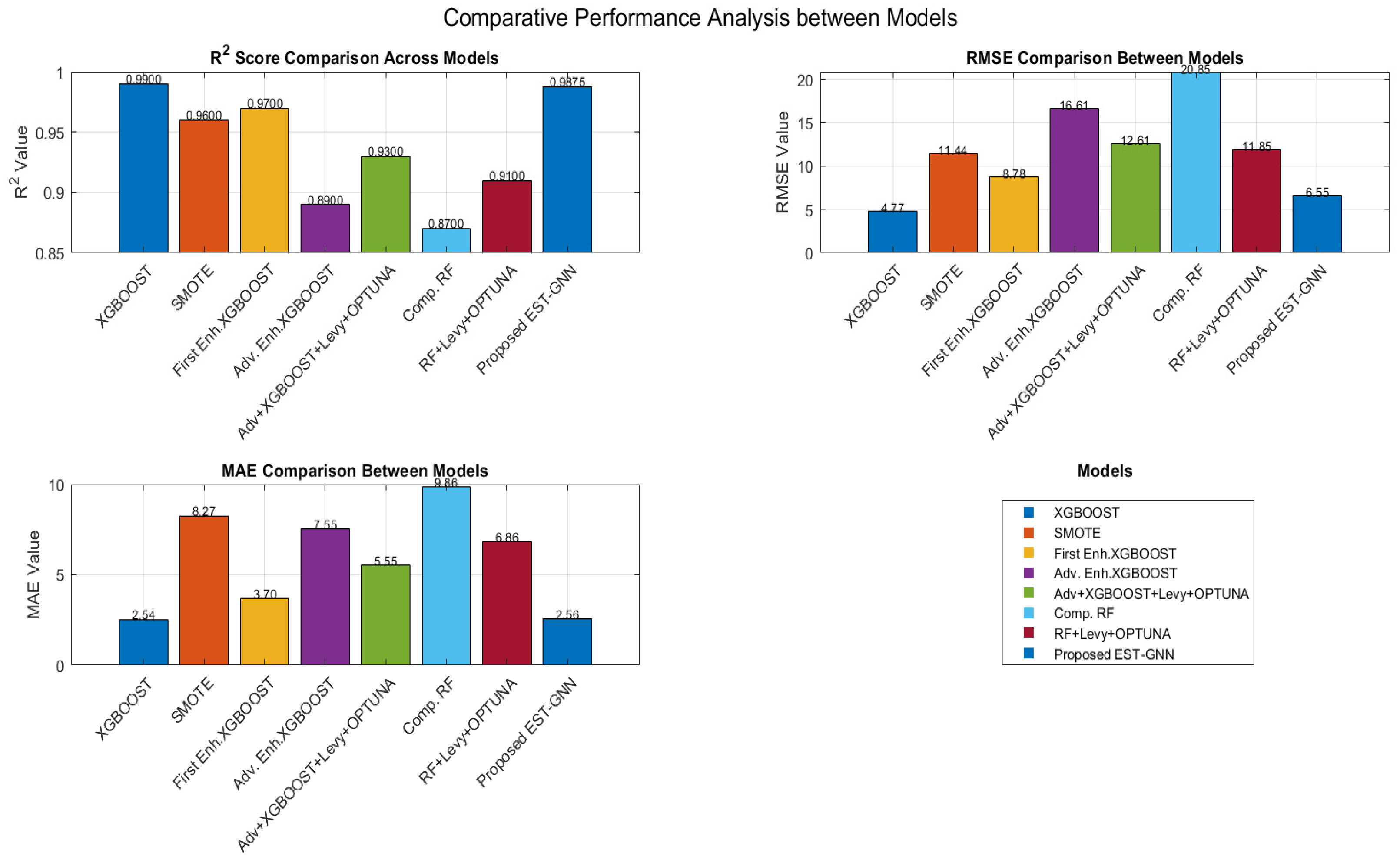
To estimate the independent contributions of model architecture to optimization approach, Lévy Flight-guided Optuna was implemented to baseline ensemble models (Table 8 and as shown in Figure 9). Despite the optimizer’s significant improvement in XGBoost’s predictive accuracy (R² = 0.89 to 0.93) and RF’s predictability from (R² = 0.87 to 0.91), these models remained less reliable than EST-GNN’s. The ability of the EST-GNN to maintain a stable R² of 0.98754 and a low MAE of 2.556 even when baselines underperform under the same optimization conditions approves that spatio-temporal relational learning and GIB-based feature cropping are the fundamental drivers of the model’s accuracy.

Table 8. Results of Best Model Performance Summary across All Results Sections.

Description	Best Model	Key Testing Metrics
One-Hot Encoded Features	XGBoost	R2 = 0.99, RMSE = 4.77, MAE = 2.54
SMOTE Techniques	Lasso Regression	R2 = 0.96, RMSE = 11.44, MAE = 8.27
First Enhanced Version	XGBoost	R2 = 0.97, RMSE = 8.78, MAE = 3.70
Advanced Enhanced Version	XGBoost	R2 = 0.89, RMSE = 16.61, MAE = 7.55
Advanced Enhanced Version followed by Lévy-Optuna	XGBoost + Lévy-Optuna	R2 = 0.93, RMSE = 12.61, MAE = 5.55
Comprehensive Feature	Random Forest	R2 = 0.87, RMSE = 20.85, MAE = 9.86
Comprehensive Feature followed by Lévy-Optuna	Random Forest + Lévy-Optuna	R2 = 0.91, RMSE = 11.85, MAE = 6.86
Proposed method (EST-GNN)	EST-GNN+ Lévy-Optuna	R2 = 0.98754, RMSE = 6.55, MAE = 2.556

Figure 9. Best model performance summary across all results sections.

By aiming at the 12 predictive features, the GIB structure, as expressed in Equation (8), resulted in a significantly more explainable model. Through this methodology, the dynamic graph was converted into a sparse representation in which the edges relate to physical emission drivers, thus satisfying the requirement for scientific explanation in the monitoring of transportation emissions. As a result of this interaction, the structure captures the physical reality of carbon emissions rather than depend on statistical objects found in traditional learning approaches.

The EST-GNN model introduces various potential advantages to traffic and emission prediction modelling, although the highest performance comes from the conventional models such as Graph Attention Networks (GAT) and Spatial-Temporal Graph Convolutional Networks (STGCN). In contrast, comparative studies have shown that these models can provide R² values between 0.89 and 0.93 on similar datasets as shown in Table 8. However, the GIB in the proposed model filters out noise and reduces fewer common features. Additionally, Lévy-Optuna optimization provides better tuning stability than traditional tuning, based on previous results. As a result, EST-GNN obtained a peak efficiency of R² = 0.98754, establishing it as a highly specialized and reliable solution for general graph models.

An empirical study was performed using only the original dataset of 7385 records to prove the validity of the predictive model and exclude biases related to data size. An R² of 0.94065 was taken without applying any data augmentation technique, indicating a high performance. A similar result was reached with the augmented dataset (R² = 0.98754), as discussed before, proving that the methodology does not establish significant synthetic bias. The structure key of predictive power consists of the optimization graph structure and Lévy-Optuna tuning process, with data augmentation operating to reduce overfitting.

5. Conclusions

The outcomes of this paper are reliable with structural models in ML theory and analytically exhibit the efficiency of combination learning methods when applied to structured datasets with complex and non-linear relationships. Models such as XGBoost and RF showed strong predictive performance by effectively balancing the bias–variance trade-off, where variance is concentrated through model cluster while preserving sufficient model expression. In distinction, linear regression-based models exhibited higher bias due to their limited capacity to capture non-linear patterns, resulting in reasonably lower performance. The superior performance of the proposed EST-GNN, which integrates spatio-temporal graph learning with Lévy Flight improved hyperparameter optimization, further proves that integrating designed relational information and the optimization mechanisms lead to more robust CO₂ emission predictions.

This paper exchanges traditional models with EST-GNN optimized via Lévy Flight-directed Optuna optimization. Realizing a state-of-the-art R² of 0.98754, the framework facilitates municipal policy formulation and fleet monitoring in real-time. While the current study applies a considerable real-world dataset of 7385 vehicle registrations, the scope is principally focused on a precise regional framework, which may limit the direct transferability of the results to significantly different urban features or driving principles. Furthermore, the model currently depends on stationary registering features; however, real-time dynamic factors such as irregular traffic density and environmental requirements could further refine emission prediction. Electrified transport and green energy grid integration are two of its practical applications.

Future research will focus on expanding the framework to incorporate real-time sensor data and edge-computing implementations on platforms such as Raspberry Pi 4s (Raspberry Pi Foundation, Cambridge, UK) for on-road behavioural monitoring, and work will be focused on hardware-level deployment onto edge AI platforms such as FPGA (Zynq Z-7010, AMD Xilinx, San Jose, CA, USA)and NVIDIA Jetson (NVIDIA Corp., Santa Clara, CA, USA) to facilitate real-time emission diagnostics. An extended objective is to investigate the integration of Hardware-In-Loop (HIL) simulations to confirm the model’s performance on more complex, multi-modal electrified transportation networks.

References

- Cha, G.-W.; Park, C.-W. Development of an optimal machine learning model to predict CO2 emissions at the building demolition stage. Buildings 2025, 15, 526. [Google Scholar] [CrossRef] [Scilit]
- Magazzino, C.; Mele, M. A new machine learning algorithm to explore the CO2 emissions-energy use-economic growth trilemma. Ann. Oper. Res. 2025, 345, 665–683. [Google Scholar] [CrossRef] [Scilit]
- Lin, X.; Hui, E.C.-M.; Shen, J. Carbon emissions reduction target and green utilization of land resources: Evidence from the industrial land market in China. Environ. Impact Assess. Rev. 2025, 110, 107677. [Google Scholar] [CrossRef] [Scilit]
- Xiao, D. Evaluating and prioritizing strategies to reduce carbon emissions in the circular economy for environmental sustainability. J. Environ. Manag. 2025, 373, 123446. [Google Scholar] [CrossRef] [Scilit]
- Yu, W.; Lin, J.; Yin, S. Drivers and forecasting of carbon emissions with extended LMDI and Bagging models: A case study of China’s Bohai Rim region. PLoS ONE 2025, 20, e0322858. [Google Scholar] [CrossRef] [Scilit]
- Zhang, G.; Ma, S.; Zheng, M.; Li, C.; Chang, F.; Zhang, F. Impact of digitization and artificial intelligence on carbon emissions considering variable interaction and heterogeneity: An interpretable deep learning modeling framework. Sustain. Cities Soc. 2025, 125, 106333. [Google Scholar] [CrossRef] [Scilit]
- Jegadeeswari, K.; Rathipriya, R. Minimizing the Carbon Footprint of Machine Learning Techniques through Sustainable AI Training Methods. In Sustainable Information Security in the Age of AI and Green Computing; IGI Global: Hershey, PE, USA, 2025; pp. 177–200. [Google Scholar]
- Hua, H.; Wu, X.; Chen, X.; Kong, H.; Sun, Y.; Yang, Q.; Tavares, M.C.; Naidoo, P. Carbon reduction oriented regional integrated energy system optimization via cloud-edge cooperative framework. CSEE J. Power Energy Syst. 2025, in press. [Google Scholar]
- Ghorbal, A.B.; Grine, A.; Elbatal, I.; Almetwally, E.M.; Eid, M.M.; El-Kenawy, E.S.M. Predicting carbon dioxide emissions using deep learning and Ninja metaheuristic optimization algorithm. Sci. Rep. 2025, 15, 4021. [Google Scholar] [CrossRef] [Scilit] [PubMed]
- Tiggeloven, J.L.; Faaij, A.P.C.; Kramer, G.J.; Gazzani, M. Optimizing Emissions Reduction in Ammonia-Ethylene Chemical Clusters: Synergistic Integration of Electrification, Carbon Capture, and Hydrogen. Ind. Eng. Chem. Res. 2025. submitted. [Google Scholar] [CrossRef] [Scilit]
- Tang, J.; Xia, L.; Huang, C. Explainable spatio-temporal graph neural networks. In Proceedings of the 32nd ACM International Conference on Information and Knowledge Management, Birmingham, UK, 21–25 October 2023. [Google Scholar]
- CO2 Emission by Vehicles. Available online: https://www.kaggle.com/datasets/debajyotipodder/co2-emission-by-vehicles/data (accessed on 10 September 2025).
- Altieri, M.; Ceci, M.; Corizzo, R. An end-to-end explainability framework for spatio-temporal predictive modeling. Mach. Learn. 2025, 114, 114. [Google Scholar] [CrossRef] [Scilit]
- Tanania, V.; Shukla, S.; Singh, S. Time series data analysis and prediction of CO2 emissions. In Proceedings of the 10th International Conference on Cloud Computing, Data Science & Engineering (Confluence), Noida, India, 29–31 January 2020; pp. 665–669. [Google Scholar]
- Wang, Y.; Tian, J.; He, L.; Zhang, Q.; Zhang, L.; Miao, S. Research on Carbon Emission Prediction Method Considering Data Preprocessing. In Proceedings of the 5th International Conference on Energy, Electrical and Power Engineering (CEEPE), Chongqing, China, 22–24 April 2022; pp. 1147–1153. [Google Scholar]
- Joshy, L.A.; Sambandam, R.K.; Vetriveeran, D.; Jenefa, J. Regression Analysis using Machine Learning Algorithms to Predict CO2 Emissions. In Proceedings of the 11th International Conference on Computing for Sustainable Global Development (INDIACom), New Delhi, India, 28 February–1 March 2024; pp. 444–448. [Google Scholar]
- Petrone, B.; Giovannardi, E.; Brusa, A.; Cavina, N.; Kitsopanidis, I. Development of an Automatic Pipeline for Data Analysis and Pre-Processing for Data Driven-Based Engine Emission Modeling in a Real Industrial Application; SAE Technical Paper; Society of Automotive Engineers (SAE): Warrendale, PA, USA, 2024. [Google Scholar]
- Kewo, A.; Manembu, P.; Nielsen, P.S. Data Pre-processing Techniques in the Regional Emission’s Load Profiles Case. In Proceedings of the 6th International Conference on Control, Decision and Information Technologies (CoDIT), Paris, France, 23–26 April 2019; pp. 2016–2021. [Google Scholar]
- Chen, Z.; Zhao, W.; Lin, X.; Han, Y.; Hu, X.; Yuan, K.; Geng, Z. Load prediction of integrated energy systems for energy saving and carbon emission based on novel multi-scale fusion convolutional neural network. Energy 2024, 290, 130181. [Google Scholar] [CrossRef] [Scilit]
- Cerda, P.; Varoquaux, G.; Kégl, B. Similarity encoding for learning with dirty categorical variables. Mach. Learn. 2018, 107, 1477–1494. [Google Scholar] [CrossRef] [Scilit]
- Lee, Z.-J.; Lin, Y.; Yang, Z.; Chen, Z.-Y.; Fan, W.-G.; Lee, C.-H. Novel automatic feature engineering for carbon emissions prediction base on deep learning. In Proceedings of the 6th Eurasian Conference on Educational Innovation (ECEI), Bangkok, Thailand, 27–29 January 2023; pp. 203–206. [Google Scholar]
- Zhang, X.; Sun, J.; Zhang, X.; Wang, F. Assessment and regression of carbon emissions from the building and construction sector in China: A provincial study using machine learning. J. Clean. Prod. 2024, 450, 141903. [Google Scholar] [CrossRef] [Scilit]
- Zhang, Y.; Liu, X.; Lei, L.; Liu, L. Estimating global anthropogenic CO2 gridded emissions using a data-driven stacked random forest regression model. Remote Sens. 2022, 14, 3899. [Google Scholar] [CrossRef] [Scilit]
- Zeng, X.; Chen, X.; Heng, L.; Oshunsanya, S.O.; Yu, H. Application of a High-Performance, Low-Cost Portable NDIR Sensor Monitoring System for Continuous Measurements of In Situ Soil CO2 Fluxes. Sensors 2026, 26, 761. [Google Scholar] [CrossRef] [Scilit]
- Joseph, V.R.; Vakayil, A. SPlit: An optimal method for data splitting. Technometrics 2022, 64, 166–176. [Google Scholar] [CrossRef] [Scilit]
- Khajavi, H.; Rastgoo, A. Predicting the carbon dioxide emission caused by road transport using a Random Forest (RF) model combined with Meta-Heuristic Algorithms. Sustain. Cities Soc. 2023, 93, 104503. [Google Scholar] [CrossRef] [Scilit]
- Akkaya, E.K.; Akkaya, A.V. Development and performance comparison of optimized machine learning-based regression models for predicting energy-related carbon dioxide emissions. Environ. Sci. Pollut. Res. 2023, 30, 122381–122392. [Google Scholar] [CrossRef] [Scilit] [PubMed]
- Hussein, A.I.; Sayed, E.H.; Aly, R.H.M. CO2 Emission Prediction Based on an Improved Swarm Optimization Technique. In Proceedings of the 1st Future International Conference on Artificial Intelligence and Cybersecurity (FICAC), Riyadh, Saudi Arabia, 15–17 December 2025. [Google Scholar]
- Karakurt, I.; Aydin, G. Development of regression models to forecast the CO2 emissions from fossil fuels in the BRICS and MINT countries. Energy 2023, 263, 125650. [Google Scholar] [CrossRef] [Scilit]
- Liao, K.; Park, E.S.; Zhang, J.; Cheng, L.; Ji, D.; Ying, Q.; Yu, J.Z. A multiple linear regression model with multiplicative log-normal error term for atmospheric concentration data. Sci. Total Environ. 2021, 767, 144282. [Google Scholar] [CrossRef] [Scilit]
- Yu, C.-H.; Gao, F.; Wen, Q.-Y. An improved quantum algorithm for ridge regression. IEEE Trans. Knowl. Data Eng. 2019, 33, 858–866. [Google Scholar] [CrossRef] [Scilit]
- Yu, F.-W.; Ho, W.-T.; Wong, C.-F.J. Predicting and decarbonizing carbon emissions from building energy use in Hong Kong: A LASSO regression approach. Energy Sustain. Dev. 2024, 78, 101374. [Google Scholar] [CrossRef] [Scilit]
- Udoh, J.; Lu, J.; Xu, Q. Application of Machine Learning to Predict CO2 Emissions in Light-Duty Vehicles. Sensors 2024, 24, 8219. [Google Scholar] [CrossRef] [Scilit]
- Mamuda, N.A.; Shabrina, A. Predicting Forest Fire Hotspots with Carbon Emission Insights Using Random Forest and Gradient Boosting Regression. Int. J. Inf. Commun. Technol. (IJoICT) 2023, 9, 137–149. [Google Scholar] [CrossRef] [Scilit]
- Patelli, L.; Cameletti, M.; Golini, N.; Ignaccolo, R. A path in regression random forest looking for spatial dependence: A taxonomy and a systematic review. In Advances in Statistical Methods for Process Monitoring, Finance, and Environmental Science; Springer: Cham, Switzerland, 2024; pp. 467–489. [Google Scholar]
- Anandhi, V.; Chezian, R.M. Support vector regression in forecasting. Int. J. Adv. Res. Comput. Commun. Eng. 2013, 2, 4148–4151. [Google Scholar]
- Xu, A.; Fang, S.; Chen, J.; Fu, Z.; Chen, Z. Carbon emission prediction based on spatial–temporal pattern recognition and novel integrated vine copula. Int. J. Environ. Sci. Technol. 2026, 23, 212. [Google Scholar] [CrossRef] [Scilit]
- Dhanka, S.; Maini, S. HyOPTXGBoost and HyOPTRF: Hybridized intelligent systems using optuna optimization framework for heart disease prediction with clinical interpretations. Multimed. Tools Appl. 2024, 83, 72889–72937. [Google Scholar] [CrossRef] [Scilit]
- Khan, M.S.; Peng, T.; Khan, M.A.; Khan, A.; Ahmad, M.; Aziz, K.; Sabri Sabri, M.M.; Abd EL-Gawaad, N.S. Explainable AutoML models for predicting the strength of high-performance concrete using Optuna, SHAP and ensemble learning. Front. Mater. 2025, 12, 1542655. [Google Scholar] [CrossRef] [Scilit]
- Chen, Y.; Li, X.; Li, E.; Zhou, J. Predicting Carbonation Depth of Recycled Aggregate Concrete Using Optuna-Optimized Explainable Machine Learning. Buildings 2026, 16, 349. [Google Scholar] [CrossRef] [Scilit]
- Xu, X.; Mao, X.; Zou, W. An improved goose optimization algorithm (I-GOOSE) based on self-adapting attenuation factors and lévy flight. Neurocomputing 2026, in press. [Google Scholar] [CrossRef] [Scilit]
- Wang, T.; Fu, Y.; Cheng, X.; Li, L.; He, Z.; Xiao, Y. Vehicle Trajectory Prediction Algorithm Based on Hybrid Prediction Model with Multiple Influencing Factors. Sensors 2025, 25, 1024. [Google Scholar] [CrossRef] [Scilit] [PubMed]
- Yassine, D.; Mustapha, J.; Naoual, B.; Hamza, E. Modeling CO2 Emissions in Morocco: A Support Vector Regression Approach. In Proceedings of the 4th International Conference on Innovative Research in Applied Science, Engineering and Technology (IRASET), Meknes, Morocco, 16–17 May 2024; pp. 1–5. [Google Scholar]
- Le, T.T.; Sharma, P.; Osman, S.M.; Dzida, M.; Nguyen, P.Q.P.; Tran, M.H.; Cao, D.N.; Tran, V.D. Forecasting energy consumption and carbon dioxide emission of Vietnam by prognostic models based on explainable machine learning and time series. Clean Technol. Environ. Policy 2024, 26, 4405–4431. [Google Scholar] [CrossRef] [Scilit]
- Król, Y.K. Sustainability Audit of University Websites in Poland: Analysing Carbon Footprint and Sustainable Design Conformity. Appl. Sci. 2025, 15, 8666. [Google Scholar] [CrossRef] [Scilit]
- Sahane, P.; Nalawade, P.; Bhamare, J.; Vaishnav, S.; Jagtap, U.; Bhosale, A. Industry-Specific Carbon Emission Reduction Techniques: A Comprehensive Survey. In Proceedings of the 8th International Conference on I-SMAC (IoT in Social, Mobile, Analytics and Cloud), Kirtipur, Nepal, 13–15 November 2024; pp. 414–420. [Google Scholar]
- Wu, F.; He, J.; Cai, L.; Du, M.; Huang, M. Accurate multi-objective prediction of CO2 emission performance indexes and industrial structure optimization using multihead attention-based convolutional neural network. J. Environ. Manag. 2023, 337, 117759. [Google Scholar] [CrossRef] [Scilit]
- Mussa, A.A.Y.; Khalifa, W.M. MLP Enhanced CO2 Emission Prediction Model with LWSSA Nature Inspired Optimization. Sci. Rep. 2025, 15, 1891. [Google Scholar] [CrossRef] [Scilit]
- Awad, A.N.; Jarad, T.S. Hybrid Particle Swarm Optimization and Feedforward Neural Network Model for Enhanced Prediction of Gas Turbine Emissions. Int. J. Energy Prod. Manag. 2024, 9, 97–105. [Google Scholar] [CrossRef] [Scilit]
- Han, Y.; Cao, L.; Geng, Z.; Ping, W.; Zuo, X.; Fan, J.; Wan, J.; Lu, G. Novel economy and carbon emissions prediction model of different countries or regions in the world for energy optimization using improved residual neural network. Sci. Total Environ. 2023, 860, 160410. [Google Scholar] [CrossRef] [Scilit] [PubMed]
- Girdhar, N.; Raj, A.; Sharma, D.; Singh, V.; Doucet, A.; Renz, M. A Comprehensive Review of Frugal Artificial Intelligence: Challenges, Applications, and the Road to Sustainable AI. Soft Comput. 2025, in press. [Google Scholar] [CrossRef] [Scilit]
- Esmaeili, A.; Ghorrati, Z.; Matson, E.T. Hierarchical collaborative hyper-parameter tuning. In International Conference on Practical Applications of Agents and Multi-Agent Systems; Springer: Cham, Switzerland, 2022; pp. 127–139. [Google Scholar]
- Chicco, D.; Warrens, M.J.; Jurman, G. The coefficient of determination R-squared is more informative than SMAPE, MAE, MAPE, MSE and RMSE in regression analysis evaluation. PeerJ Comput. Sci. 2021, 7, e623. [Google Scholar] [CrossRef] [Scilit]
- Salmanpour, M.R.; Alizadeh, M.; Mousavi, G.; Sadeghi, S.; Amiri, S.; Oveisi, M.; Rahmim, A.; Hacihaliloglu, I. Machine Learning Evaluation Metric Discrepancies Across Programming Languages and Their Components in Medical Imaging Domains: Need for Standardization. IEEE Access 2025, in press. [Google Scholar]
Disclaimer/Publisher’s Note: The statements, opinions and data contained in all publications are solely those of the individual author(s) and contributor(s) and not of MDPI and/or the editor(s). MDPI and/or the editor(s) disclaim responsibility for any injury to people or property resulting from any ideas, methods, instructions or products referred to in the content. |
© 2026 by the authors. Licensee MDPI, Basel, Switzerland. This article is an open access article distributed under the terms and conditions of the Creative Commons Attribution (CC BY) license.