Co-Design of Structural Parameters and Motion Planning in Serial Manipulators via SAC-Based Reinforcement Learning

Abstract

In the context of Industry 4.0 and intelligent manufacturing, conventional serial manipulators face limitations in dynamic task environments due to fixed structural parameters and the traditional decoupling of mechanism design from motion planning. To address this issue, this study proposes SAC-SC (Soft Actor–Critic-based Structure–Control Co-Design), a reinforcement learning framework for the co-design of manipulator link lengths and motion planning policies. The approach is implemented on a custom four-degree-of-freedom PRRR manipulator with manually adjustable link lengths, where a hybrid action space integrates configuration selection at the beginning of each episode with subsequent continuous joint-level control, guided by a multi-objective reward function that balances task accuracy, execution efficiency, and obstacle avoidance. Evaluated in both a simplified kinematic simulator and the high-fidelity MuJoCo physics engine, SAC-SC achieves 100% task success rate in obstacle-free scenarios and 85% in cluttered environments, with a planning time of only 0.145 s per task, over 15 times faster than the two-stage baseline. The learned policy also demonstrates zero-shot transfer between simulation environments. These results indicate that integrating structural parameter optimization and motion planning within a unified reinforcement learning framework enables more adaptive and efficient robotic operation in unstructured environments, offering a promising alternative to conventional decoupled design paradigms.

1. Introduction

As manufacturing evolves from Industry 4.0 towards Industry 5.0, there is a growing emphasis on human-centric, adaptive, and resilient robotic systems that can seamlessly collaborate with human workers in unstructured and dynamic environments. In this context, conventional serial manipulators—despite their success in automated settings—face fundamental limitations due to fixed structural parameters and the traditional decoupling of mechanism design from motion planning. Their rigidity prevents them from adapting to varying task requirements, human preferences, or unforeseen workspace changes, which are central challenges in Industry 5.0 scenarios such as collaborative assembly, personalized production, and flexible logistics.

Consequently, even when equipped with advanced motion planners or modern reinforcement learning controllers [1,2,3], these robots may fail in dynamic scenarios: they can become kinematically incapable of reaching the target, trapped in singular configurations, or unable to generate collision-free trajectories—ultimately leading to task failure.

To overcome this limitation, recent efforts have explored co-design approaches that jointly optimize morphology and control. Yet, existing methods either rely on external optimizers, require differentiable dynamics models, treat morphology as a passive input, or restrict design variables to discrete sets. Crucially, none embed continuous structural parameters directly into the reinforcement learning action space for end-to-end, per-episode co-adaptation of morphology and control—a capability essential for responsive manipulation in dynamic environments.

To address this gap, we propose SAC-SC (Soft Actor–Critic-based Structure–Control Co-Design), a unified reinforcement learning framework for the end-to-end co-design of structural parameters and motion planning in serial manipulators. Our approach is implemented on a custom four-degree-of-freedom Prismatic-Revolute-Revolute-Revolute (PRRR) manipulator developed at Tongji University, whose second, third, and fourth link lengths can be actively adjusted via servo-driven linear actuators. SAC-SC uniquely embeds these continuous link lengths into the action space of a Soft Actor–Critic policy. At the beginning of each episode, the agent selects an optimal morphology and initiates a corresponding motion strategy; once set, the configuration remains fixed while the policy executes continuous joint-level control to complete the task. A composite reward function balances task accuracy, execution efficiency, collision avoidance, end-effector reachability, and joint effort. By leveraging SAC’s maximum-entropy objective, our framework encourages exploration across diverse morphology-control combinations, facilitating the discovery of high-performing solutions in complex design spaces.

The main contributions of this work are threefold:

(1)

We propose a novel formulation that embeds continuous structural parameters (link lengths) into the reinforcement learning action space, where they are determined once per episode and remain fixed during execution;

(2)

We develop an integrated training scheme that jointly optimizes configuration selection and trajectory generation within a single end-to-end policy, eliminating iterative design loops;

(3)

We provide comprehensive empirical validation on a custom 4-DOF PRRR manipulator designed and built by our team at the Industry 4.0 Laboratory (Tongji University, Shanghai, China), demonstrating high success rates, fast planning (<0.15 s), and consistent performance in both obstacle-free and cluttered environments, along with zero-shot transfer to a high-fidelity physics simulator.

2. Related Work

2.1. Structural Design and Kinematic Optimization of Serial Manipulators

Significant progress has been made in the offline optimization of serial manipulator morphology under static task assumptions. Researchers commonly define composite performance metrics that integrate kinematic criteria—such as Jacobian condition number, global dexterity, and energy consumption—and optimize them using evolutionary algorithms like genetic algorithms [4] or particle swarm optimization [5]. Separately, recent studies have explored multi-objective trajectory planning to minimize energy consumption, operational cost, and task completion time in simulation environments [6]. While effective for predefined scenarios, these approaches are computationally intensive and inherently incapable of supporting online reconfiguration. Crucially, they treat morphology design as a one-time, open-loop process, decoupled from the subsequent motion planning stage.

2.2. Motion Planning and Control for Fixed-Morphology Manipulators

In parallel, motion planning and control have advanced significantly under the assumption of a fixed robot structure. Sampling-based planners such as RRT* [7,8] and graph-search methods like A* [9] have become standard tools for generating collision-free trajectories in high-dimensional configuration spaces. Complementary to these geometric approaches, optimization-based methods focus on trajectory smoothness by minimizing higher-order kinematic derivatives through polynomial interpolation or direct optimization [10]. More recently, deep reinforcement learning (DRL) methods—including Deep Deterministic Policy Gradient (DDPG) [11] and Soft Actor–Critic (SAC) [12]—have demonstrated remarkable adaptability in dynamic manipulation tasks such as grasping [13], assembly [14], and redundant arm control [15]. However, the performance of all these controllers remains fundamentally constrained by the pre-defined mechanical structure; no amount of policy adaptation can overcome inherent kinematic limitations such as insufficient reach or unavoidable singularities.

2.3. Co-Design of Morphology and Control in Robotics

To overcome the limitations of sequential design, the field has increasingly embraced co-design—jointly optimizing morphology and control in a closed loop. Early efforts introduced surrogate models, such as control proxy functions, to approximate controller performance during structural optimization [16]. Subsequent work enhanced robustness by evaluating combinations of actuator parameters and model predictive controllers through Monte Carlo sampling under model uncertainty [17]. Reinforcement learning has also been integrated into co-design: for example, discrete leg-length ratios in quadrupedal locomotion were evaluated using PPO [18,19], and hybrid frameworks combining genetic algorithms with RL were proposed for multi-arm systems [20]. However, these methods did not embed morphological parameters directly into the policy network. More recent directions include end-to-end differentiable co-design frameworks that perform gradient-based optimization over differentiable simulators [21], as well as morphology-aware policies that encode fixed topologies into graph neural networks [22]. Despite their advances, existing approaches either rely on external optimizers, require differentiable dynamics models, treat morphology as a passive input feature, or restrict design variables to discrete sets—leaving a gap for an end-to-end, sample-based RL framework that enables continuous, per-episode co-adaptation of structure and control.

3. A 4-DOF PRRR Manipulator System

This section presents the technical foundation of our experimental platform and modeling framework. We first describe the mechanical design and variable-link architecture of the custom 4-DOF PRRR manipulator. Subsequently, we derive its forward and inverse kinematics using the Denavit–Hartenberg (D–H) convention, and formulate the geometric Jacobian matrix. These analytical models underpin both the simulation environment and the reward function design in our SAC-SC framework, ensuring kinematic consistency and enabling efficient policy learning.

3.1. Robot System and Variable Link Parameters

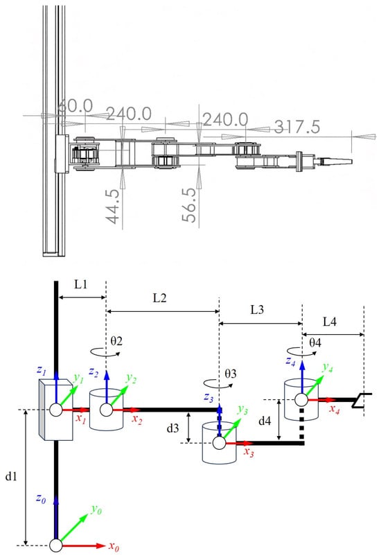
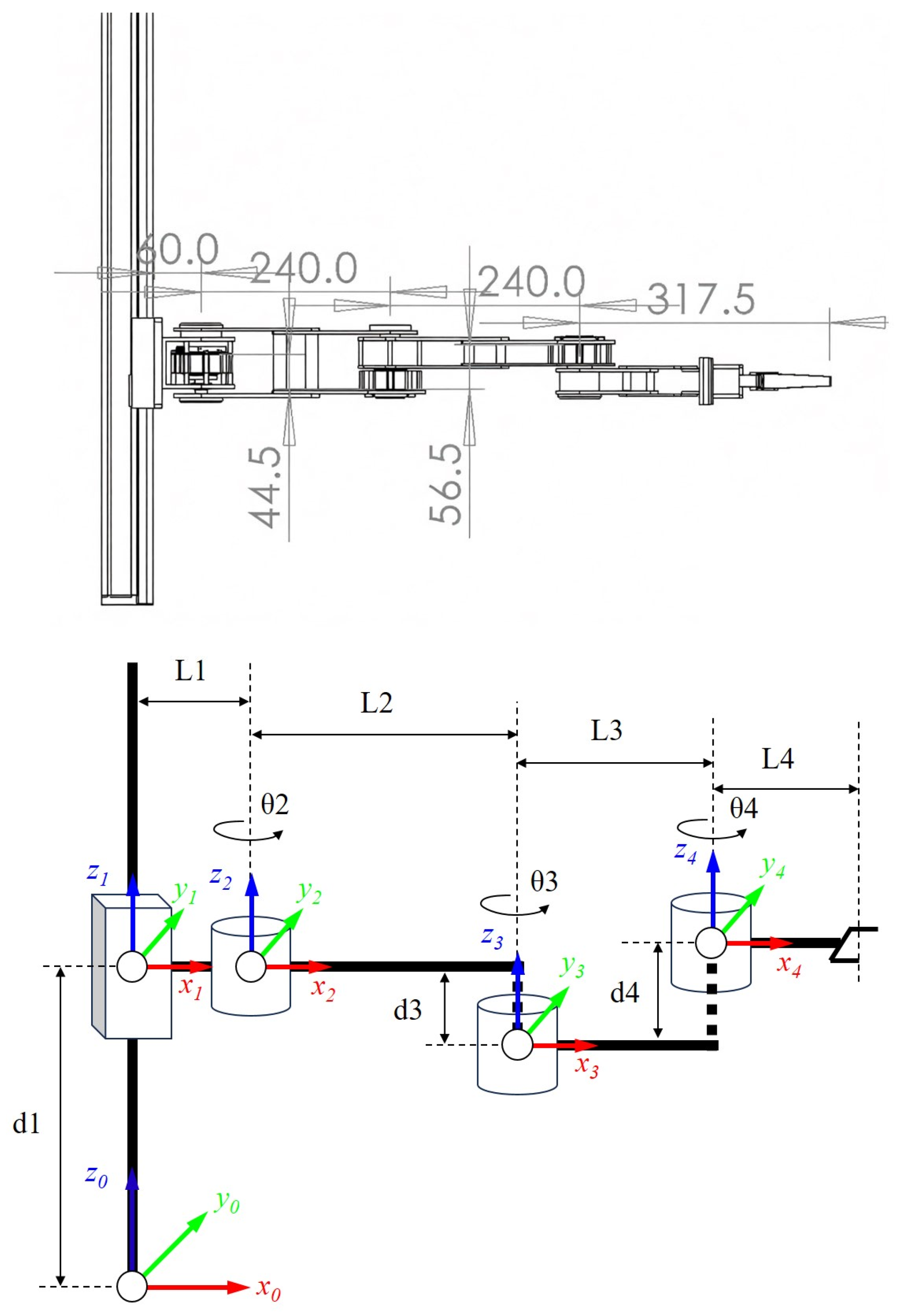
We present a custom-designed 4-DOF serial manipulator developed at Tongji University, featuring manually adjustable link lengths for reconfigurable manipulation. This study investigates a four-degree-of-freedom (4-DOF) serial manipulator with variable link lengths, denoted as the PRRR manipulator. As shown in Figure 1, the kinematic chain consists of one prismatic joint (P) followed by three revolute joints (R₁–R₃), forming a PRRR architecture. The lengths of links 2 to 4—denoted L2, L3, and L4—are manually adjustable via clamping mechanisms. This design prioritizes low cost, high structural rigidity, and experimental accessibility while enabling configuration adaptation for diverse tasks and dynamic environments.

Figure 1. Kinematic structure of the 4-DOF PRRR manipulator with D-H parameterization.

The Denavit–Hartenberg (D–H) convention is adopted to assign coordinate frames to each joint. The corresponding D–H parameters are listed in Table 1. Substituting these parameters into the standard homogeneous transformation yields the pose relationship between adjacent frames.

Table 1. Denavit-Hartenberg parameters of the 4-DOF PRRR manipulator.

Joint No.	Joint Type	di (m)	ai−1 (m)	θi (deg)	αi−1 (deg)
1	Prismatic	d1	L1	0	0
2	Revolute	0	L2	θ2	0
3	Revolute	d2	L3	θ3	0
4	Revolute	d3	L4	θ4	0

3.2. Forward Kinematics

To establish the kinematic model of the PRRR manipulator, the Denavit–Hartenberg (D–H) convention is employed to systematically define coordinate frames along the kinematic chain. This formulation enables the derivation of homogeneous transformation matrices that relate successive joint frames, ultimately yielding the end-effector pose with respect to the base frame.

The homogeneous transformation from frame i to frame i − 1 is given by:

$${}_{i }{}^{i-1}T_m=\left[\begin{array}{cccc}\cos {\theta }_i& -\sin {\theta }_i\cos {\alpha }_i& \sin {\theta }_i\sin {\alpha }_i& a_i\cos {\theta }_i\\ \sin {\theta }_i& \cos {\theta }_i\cos {\alpha }_i& -\cos {\theta }_i\sin {\alpha }_i& a_i\sin {\theta }_i\\ 0& \sin {\alpha }_i& \cos {\alpha }_i& d_i\\ 0& 0& 0& 1\end{array}\right]\hspace{1em}$$

(1)

Given α_i = 0 for all joints, the individual transformations simplify to:

$${}_1{}^{0}T_m=\left[\begin{array}{cccc}1& 0& 0& L_1\\ 0& 1& 0& 0\\ 0& 0& 1& d_1\\ 0& 0& 0& 1\end{array}\right]\hspace{1em}$$

(2)

$${}_2{}^{1}T_m=\left[\begin{array}{cccc}\cos {\theta }_2& -\sin {\theta }_2& 0& L_2\cos {\theta }_2\\ \sin {\theta }_2& \cos {\theta }_2& 0& L_2\sin {\theta }_2\\ 0& 0& 1& 0\\ 0& 0& 0& 1\end{array}\right]\hspace{1em}$$

(3)

$${}_3{}^{2}T_m=\left[\begin{array}{cccc}\cos {\theta }_3& -\sin {\theta }_3& 0& L_3\cos {\theta }_3\\ \sin {\theta }_3& \cos {\theta }_3& 0& L_3\sin {\theta }_3\\ 0& 0& 1& d_3\\ 0& 0& 0& 1\end{array}\right]\hspace{1em}$$

(4)

$${}_4{}^{3}T_m=\left[\begin{array}{cccc}\cos {\theta }_4& -\sin {\theta }_4& 0& L_4\cos {\theta }_4\\ \sin {\theta }_4& \cos {\theta }_4& 0& L_4\sin {\theta }_4\\ 0& 0& 1& d_4\\ 0& 0& 0& 1\end{array}\right]$$

(5)

The end-effector pose relative to the base frame is obtained as:

$${}_4{}^{0}T_m={}_1{}^{0}T_m\cdot {}_2{}^{1}T_m\cdot {}_3{}^{2}T_m\cdot {}_4{}^{3}T_m=\left[\begin{array}{cccc}{n}_x& o_x& a_x& P_x\\ n_y& o_y& a_y& P_y\\ n_z& o_z& a_z& P_z\\ 0& 0& 0& 1\end{array}\right]$$

(6)

The orientation columns correspond to the normal (n), orientation (o), and approach (a) vectors of the end-effector frame, while [P_x, P_y, P_z]^T denotes its position. Using trigonometric identities, the position components simplify to:

$$\begin{array}{l}{P}_x=L_1+L_2\cos {\theta }_2+L_3\cos ({\theta }_2+{\theta }_3)+L_4\cos ({\theta }_2+{\theta }_3+{\theta }_4),\hfill \\ P_y=L_2\sin {\theta }_2+L_3\sin ({\theta }_2+{\theta }_3)+L_4\sin ({\theta }_2+{\theta }_3+{\theta }_4),\hfill \\ P_z=d_1+d_3+d_4.\hfill \end{array}$$

(7)

The orientation vectors satisfy a_x = a_y = 0, a_z = 1, and n_z = o_z = 0, consistent with all joint axes being parallel to the global Z-axis.

3.3. Inverse Kinematics

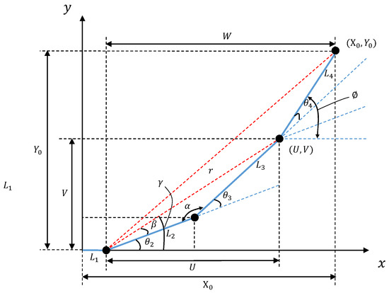
Given a desired end-effector pose (X₀, Y₀, Z₀, ϕ), where ϕ is the orientation about the Z-axis, the inverse kinematics problem seeks joint variables [d₁, θ₂, θ₃, θ₄]. Since only the prismatic joint contributes to vertical motion, d₁ = Z₀. The rotational joints lie in the XY-plane, and the end-effector orientation satisfies $\varphi ={\theta }_2+{\theta }_3+{\theta }_4$. Define intermediate variables based on the planar projection (Figure 2):

$$\begin{array}{ccc}W& =& X_0-L_1,\\ U& =& W-L_4\cos \varphi ,\\ V& =& Y_0-L_4\sin \varphi .\end{array}$$

(8)

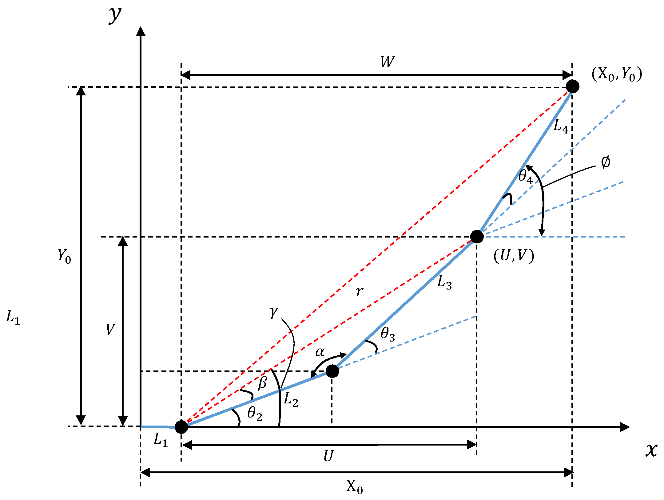
Figure 2. Geometric configuration of the PRRR manipulator in the XY plane for inverse kinematic analysis. The blue solid lines represent the physical links of the 4-DOF PRRR manipulator, with each segment corresponding to a jointed arm link. Dashed lines are auxiliary construction lines used for geometric illustration.

The distance $r=\sqrt{U^2+V^2}$ forms a triangle with sides L₂ and L₃. Applying the law of cosines gives two possible solutions for θ₃:

$${\theta }_3=\pm {\cos }^{-1}\left({\displaystyle \frac{U^2+V^2-L_2^2-L_3^2}{2L_2{L}_3}}\right)$$

(9)

Let $\gamma ={\tan }^{-1}(U/V)$ and $\beta ={\tan }^{-1}\left({\displaystyle \frac{L_3\sin {\theta }_3}{L_2+L_3\cos {\theta }_3}}\right)$. Then,

$${\theta }_2=\gamma -\beta ={\tan }^{-1}\left({\displaystyle \frac{U}{V}}\right)-{\tan }^{-1}\left({\displaystyle \frac{L_3\sin {\theta }_3}{L_2+L_3\cos {\theta }_3}}\right)$$

(10)

Finally,

$${\theta }_4=\varphi -{\theta }_2-{\theta }_3$$

(11)

This yields a closed-form inverse kinematic solution with two configurations (elbow-up/down).

3.4. Jacobian Matrix

The Jacobian matrix plays a central role in robotic manipulation, bridging joint-space velocities and task-space (Cartesian) motion of the end-effector. For the 4-DOF PRRR manipulator, it enables critical analyses such as velocity transformation, singularity identification, and real-time trajectory generation—particularly important given the system’s adjustable link lengths and resulting variable workspace geometry.

Let $\stackrel{.}{p}={[{\dot{P}}_x,{\dot{P}}_y,{\dot{P}}_z]}^T$ denote the end-effector position derived from Equation (1), and $\stackrel{.}{q}={[d_1,{\theta }_2,{\theta }_3,{\theta }_4]}^T$ the joint velocity vector. The linear velocity of the end-effector, $\stackrel{.}{p}$, is related to $\stackrel{.}{q}$ through the geometric Jacobian $J\in {ℝ}^{3\times 4}$:

$$\stackrel{.}{p}=J\stackrel{.}{q}$$

(12)

The Jacobian entries are obtained by partial differentiation of the position components:

$$J=\left[\begin{array}{cccc}0& {\displaystyle \frac{\mathsf{\partial }{P}_x}{\mathsf{\partial }{\theta }_2}}& {\displaystyle \frac{\mathsf{\partial }{P}_x}{\mathsf{\partial }{\theta }_3}}& {\displaystyle \frac{\mathsf{\partial }{P}_x}{\mathsf{\partial }{\theta }_4}}\\ 0& {\displaystyle \frac{\mathsf{\partial }{P}_y}{\mathsf{\partial }{\theta }_2}}& {\displaystyle \frac{\mathsf{\partial }{P}_y}{\mathsf{\partial }{\theta }_3}}& {\displaystyle \frac{\mathsf{\partial }{P}_y}{\mathsf{\partial }{\theta }_4}}\\ 1& 0& 0& 0\end{array}\right]$$

(13)

where

$$\begin{array}{l}{\displaystyle \frac{\mathsf{\partial }{P}_x}{\mathsf{\partial }{\theta }_2}}=-L_2\sin {\theta }_2-L_3\sin ({\theta }_2+{\theta }_3)-L_4\sin ({\theta }_2+{\theta }_3+{\theta }_4),\hfill \\ {\displaystyle \frac{\mathsf{\partial }{P}_x}{\mathsf{\partial }{\theta }_3}}=-L_3\sin ({\theta }_2+{\theta }_3)-L_4\sin ({\theta }_2+{\theta }_3+{\theta }_4),\hfill \\ {\displaystyle \frac{\mathsf{\partial }{P}_x}{\mathsf{\partial }{\theta }_4}}=-L_4\sin ({\theta }_2+{\theta }_3+{\theta }_4),\hfill \\ {\displaystyle \frac{\mathsf{\partial }{P}_y}{\mathsf{\partial }{\theta }_2}}=L_2\cos {\theta }_2+L_3\cos ({\theta }_2+{\theta }_3)+L_4\cos ({\theta }_2+{\theta }_3+{\theta }_4),\hfill \\ {\displaystyle \frac{\mathsf{\partial }{P}_y}{\mathsf{\partial }{\theta }_3}}=L_3\cos ({\theta }_2+{\theta }_3)+L_4\cos ({\theta }_2+{\theta }_3+{\theta }_4),\hfill \\ {\displaystyle \frac{\mathsf{\partial }{P}_y}{\mathsf{\partial }{\theta }_4}}=L_4\cos ({\theta }_2+{\theta }_3+{\theta }_4).\hfill \end{array}$$

(14)

Due to its 3 × 4 Jacobian structure, the manipulator is kinematically redundant and may encounter singular configurations where rank(J) < 3, limiting motion capability in certain Cartesian directions. The Moore–Penrose pseudoinverse J^† provides a robust means to resolve this redundancy and compute feasible joint velocities for trajectory tracking:

$$\stackrel{.}{q}=J^{†}\stackrel{.}{p}$$

(15)

This theoretical framework provides the mathematical foundation for subsequent numerical inverse kinematics solutions and real-time trajectory planning based on the Jacobian matrix.

4. SAC-SC: Co-Design of Structural Parameters and Path Planning

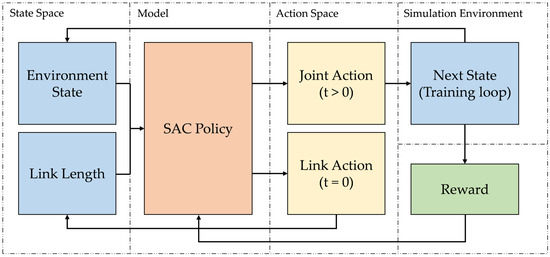
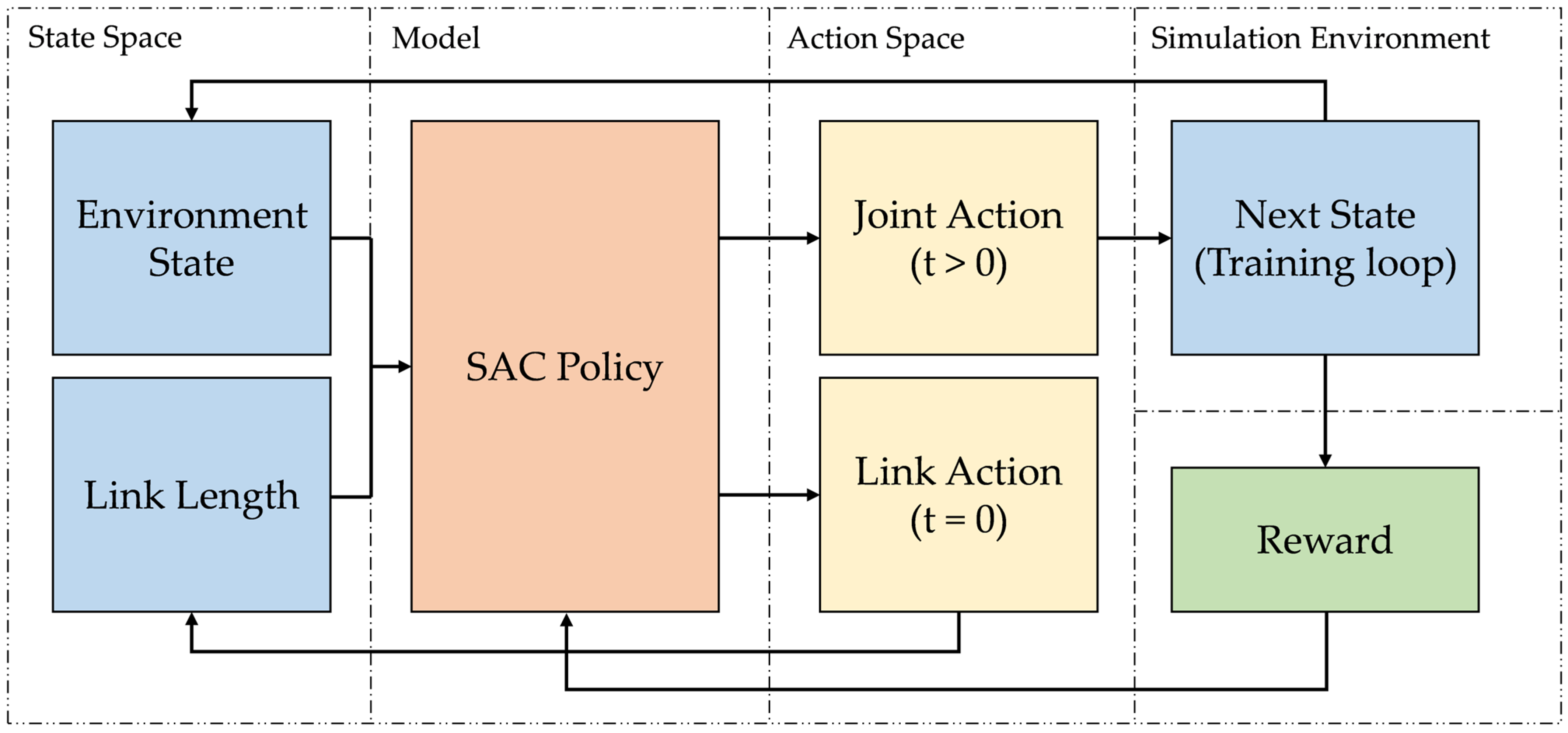
This section presents the end-to-end reinforcement learning framework for co-designing morphology and motion planning in serial manipulators. As illustrated in Figure 3, the SAC policy receives a composite state input comprising both the environment state (e.g., goal pose and obstacle positions) and the current link lengths. At the beginning of each episode (t = 0), the policy selects a set of continuous link lengths—defining the robot’s morphological configuration—which remains fixed throughout the task execution. Subsequently, at each time step (t > 0), the same policy generates joint-level control actions to navigate the end-effector toward the target while avoiding collisions. The resulting next state is fed back into the policy, and a composite reward function evaluates task success, efficiency, safety, and kinematic feasibility. This architecture enables seamless integration of structural design and trajectory generation within a single learning process.

Figure 3. System architecture of the SAC-SC framework. The SAC policy takes as input the environment state and current link lengths. At t = 0, it outputs a morphology action (link length selection); at t > 0, it outputs joint controls.

4.1. The SAC-SC Framework

We propose SAC-SC (Structure–Control Soft Actor–Critic), a reinforcement learning framework that unifies the selection of manipulator structural parameters and path planning into a single end-to-end decision process. Built upon the standard Soft Actor–Critic (SAC) algorithm [12], SAC-SC retains SAC’s core architecture—including dual Q-networks, entropy-regularized policy updates, and off-policy training—but fundamentally redefines the state representation, action space, and reward structure to enable co-design of geometry and motion.

Specifically, while SAC is originally designed for pure control tasks with fixed system dynamics, SAC-SC extends it to a design-control co-adaptation setting by treating link lengths as slow-time-scale action variables. The policy thus learns not only how to move, but also how to configure the robot for a given task. Below, we first briefly review the SAC foundation, then detail our problem-specific formulations.

SAC adopts a maximum entropy RL framework, which simultaneously maximizes the expected cumulative reward and the entropy of the policy. This dual objective encourages the agent to explore diverse behaviors while maintaining task performance—a property particularly advantageous for high-dimensional continuous control problems.

Formally, the optimization problem is expressed as:

$$J(\pi )={\displaystyle \sum _{t=0}^T{\mathbb{E}}_{(s_t,a_t)~{\rho }_{\pi }}}\left[r(s_t,a_t)+\alpha \mathcal{H}(\pi (\cdot \mid s_t))\right]$$

(16)

where $r(s_t,a_t)$ denotes the reward function, $\mathcal{H}(\pi (\cdot \mid s_t))$ is the policy entropy, α > 0 is a temperature parameter that balances performance and exploration, and γ ∈ (0, 1) is the discount factor.

SAC employs an Actor–Critic architecture. The Critic consists of two soft Q-networks $Q_{\theta }(s,a)$ that estimate the state-action value function. Their parameters $\theta$ are updated by minimizing the Bellman residual:

$$J_Q(\theta )={\mathbb{E}}_{(s_t,a_t)~D}\left[{\displaystyle \frac{1}{2}}{\left(Q_{\theta }(s_t,a_t)-\widehat{Q}(s_t,a_t)\right)}^2\right]$$

(17)

where D is the replay buffer and ϕ⁻ ${\theta }^{-}$ denotes the parameters of the target network.

The Actor (policy network ${\pi }_{\varphi }$) is updated by minimizing the policy loss:

$$J_{\pi }(\varphi )={\mathbb{E}}_{s_t~D,{ϵ}_t~\mathcal{N}}\left[\alpha \log {\pi }_{\varphi }(f_{\varphi }({ϵ}_t;s_t)\mid s_t)-Q_{\theta }(s_t,f_{\varphi }({ϵ}_t;s_t))\right]$$

(18)

where the reparameterization trick is used to enable gradient backpropagation through stochastic sampling:

$$a={\mu }_{\theta }(s)+ϵ{\sigma }_{\theta }(s),ϵ~\mathcal{N}(0,I)$$

(19)

In this work, we adopt the standard SAC implementation without modifications to its network architecture or update rules. The key innovation lies not in the algorithm itself, but in how the problem is formulated: we unify the selection of variable link parameters and subsequent path planning into a single end-to-end RL problem. By carefully designing the state representation, hybrid action space, and staged reward function, the SAC policy is guided to jointly learn how to configure the manipulator’s geometry and how to execute an efficient trajectory under that configuration. The algorithm’s native support for continuous actions and its intrinsic entropy-driven exploration make it ideally suited for this joint optimization task.

4.2. Parameterized Path Planning: Scenario and Problem Definition

We model the co-design of mechanism parameters and motion planning as a Markov Decision Process (MDP). A defining feature of this MDP is its two-phase decision structure: at the start of each episode, the agent selects a fixed set of mechanical parameters; subsequently, it performs a complete path-planning task under that static configuration. This reflects the physical reality that structural adjustments (e.g., link lengths) are performed offline, while motion execution occurs online. The following subsections detail the key components of this formulation.

4.2.1. Workspace

The workspace, defined as the set of all end-effector positions reachable under a given parameter configuration, is a fundamental geometric property that governs task feasibility. For the PRRR manipulator with adjustable link lengths L2, L3, L4, the workspace dynamically varies: increasing link lengths expands the reachable volume but may introduce kinematic redundancy or singular configurations, whereas shorter links enhance local dexterity at the expense of coverage.

In this study, workspace properties are not directly optimized; instead, they are implicitly shaped through the reward signal and environment constraints. To ensure physical validity, the environment performs a reachability validation during the reset phase: only if the randomly sampled target position xtarget target position lies within the current workspace is the episode allowed to proceed. Otherwise, the environment is immediately reset to avoid training on infeasible configurations.

4.2.2. State Space

The state at time step t is defined as:

$$a={\mu }_{\theta }(s)+ϵ{\sigma }_{\theta }(s),ϵ~\mathcal{N}(0,I)$$

(20)

where $p\in {ℝ}^{n_p}$ denotes the selected link parameters (e.g., L2, L3, L4) for the current episode; $q_t\in {ℝ}^{n_q}$ represents the current joint configuration (angles or displacements); $o_t=x_{\mathrm{target}}\in {ℝ}^3$ is the goal observation.

Critically, p is determined at t = 0 and remains constant throughout the episode, consistent with the physical constraint that mechanical parameters cannot be adjusted during task execution.

4.2.3. Action Space

The action space exhibits temporal dependency and is structured as a hybrid continuous space: At t = 0: the agent outputs a parameter-adjustment action $a_0=\mathrm{\Delta }p\in {\mathcal{A}}_p$, yielding the final configuration $p=p_{\mathrm{init}}+\mathrm{\Delta }p$. For $t\ge 1$: the agent outputs a motion-control action $a_t=\mathrm{\Delta }q\in {\mathcal{A}}_q$, typically joint velocities. Integration of distinct action spaces from both phases into a unified hybrid action space:

$$a_t=\left\{\begin{array}{ll}[a_p,a_q]\in {\mathcal{A}}_p\times {\mathcal{A}}_q,\hfill & t=0,\hfill \\ [0,a_q]\in \left\{0\right\}\times {\mathcal{A}}_q,\hfill & t\ge 1,\hfill \end{array}\right.$$

(21)

The complete action space is thus:

$$\mathcal{A}={\mathcal{A}}_p\times {\mathcal{A}}_q\subset {ℝ}^{n_p+n_q}$$

(22)

where both ${\mathcal{A}}_p$ and ${\mathcal{A}}_q$ are bounded continuous domains. During inference, the Actor network outputs a single vector, which is interpreted conditionally based on the time step. The Critic network, however, always receives the full state–action pair, enabling it to assess the long-term impact of early parameter decisions.

4.2.4. Simplified Kinematic Simulation Environment

To enable rapid prototyping and efficient policy learning, a lightweight simulation environment is developed based on analytical forward kinematics and compliant with the OpenAI Gym interface. This environment abstracts away dynamic effects such as inertia and friction, focusing solely on kinematic feasibility to reduce computational cost while preserving geometric correctness.

The environment models the 4-DOF PRRR manipulator, with link lengths L2, L3, L4 continuously adjustable within predefined bounds. At episode initialization, the agent outputs normalized parameter adjustments, which are linearly scaled to physical ranges. Joint velocity commands then drive the arm toward the target, with the end-effector position computed in real time using:

$$\begin{array}{l}{P}_x=L_1+L_2\cos {\theta }_2+L_3\cos ({\theta }_2+{\theta }_3)+L_4\cos ({\theta }_2+{\theta }_3+{\theta }_4),\hfill \\ P_y=L_2\sin {\theta }_2+L_3\sin ({\theta }_2+{\theta }_3)+L_4\sin ({\theta }_2+{\theta }_3+{\theta }_4),\hfill \\ P_z=d_1+d_3+d_4.\hfill \end{array}$$

(23)

where $d_1\in [0.1,0.5]\mathrm{m}$ and ${\theta }_i\in \left[-{\displaystyle \frac{\pi }{2}},{\displaystyle \frac{\pi }{2}}\right]$. Target positions are sampled exclusively from the verified reachable workspace to guarantee task feasibility.

The environment supports two operational modes: Training mode: random targets and parameter adjustments for policy learning; Testing mode: fixed targets and manual parameter settings for ablation studies and visualization.

The state vector is 10-dimensional (3 for p, 4 for q, 3 for xtarget), and the action vector is 7-dimensional (3 for Δp, 4 for Δq). This simulator serves as the primary platform for initial policy development before transfer to high-fidelity environments.

4.2.5. Reward Functions

The reward function is carefully designed to guide the agent toward jointly optimizing configuration and motion. After extensive empirical tuning, the total reward is composed of five components:

$$r_t=r_{\mathrm{dist}}+r_{\mathrm{succ}}+r_{\mathrm{prog}}+r_{\mathrm{time}}+r_{\mathrm{eff}}$$

(24)

defined as follows:

Nonlinear distance reward:

$$r_{\mathrm{dist}}=\left\{\begin{array}{ll}0,\hfill & \mathrm{if} d<0.001,\hfill \\ 8\exp (-2d)-5+1000(0.01-d),\hfill & \mathrm{if} 0.001\le d<0.01,\hfill \\ 8\exp (-2d)-5,\hfill & \mathrm{if} d\ge 0.01.\hfill \end{array}\right.$$

(25)

This provides strong gradients at large distances while saturating near the goal to prevent oscillation.

Success reward:

$$r_{\mathrm{succ}}=\left\{\begin{array}{ll}200,\hfill & \mathrm{if} d<0.001,\hfill \\ 0,\hfill & \mathrm{otherwise}.\hfill \end{array}\right.$$

(26)

Progress reward:

$$r_{\mathrm{prog}}=\left\{\begin{array}{ll}\min (5(d_{t-1}-d_t),\hspace{0.33em}2.0),\hfill & \mathrm{if} d_{t-1}-d_t>0.001,\hfill \\ 0,\hfill & \mathrm{otherwise}.\hfill \end{array}\right.$$

(27)

Time penalty:

$$r_{\mathrm{time}}=-0.1$$

(28)

Efficiency reward (granted only upon success): Let $J_{\mathrm{total}}={\displaystyle \sum _{t=1}^T\Vert \mathrm{\Delta }{q}_t\Vert }$ denote the total joint effort. Then,

$$r_{\mathrm{eff}}={\displaystyle \frac{200}{J_{\mathrm{total}}}}$$

(29)

Notably, no explicit reward term is included for workspace size, manipulability, or other kinematic metrics. Empirical evaluation confirms that the above task-oriented rewards are sufficient to induce high-performance parameter configurations implicitly; adding explicit shaping terms was found to interfere with end-to-end learning.

4.3. Training Protocol and Implementation Details

Training is implemented in Python 3.12 using the Stable-Baselines3 library (version 2.6.0) with the standard SAC algorithm. Key hyperparameters are tuned for stability and efficiency, as shown in Table 2:

• Network architecture: MLP with two hidden layers of 1024 units each for both Actor and Critic;
• Activation function: all hidden layers use ReLU activation, while the policy output layer uses a tanh activation;
• Learning rate: 3 × 10⁻⁵;
• Replay buffer size: 1,000,000 transitions;
• Batch size: 512;
• Training frequency: update every 4 environment steps, with 2 gradient steps per update;
• Target network update rate: τ = 0.005;
• Discount factor: γ = 0.95;
• Initial policy log-standard deviation: −2.0;
• Learning start steps: 10,000.

Table 2. Hyperparameters of the SAC-SC algorithm used in training.

Parameter Name	Value
Network architecture	[1024, 1024]
Activation function	ReLU (hidden), tanh (policy output)
Initial policy log-standard deviation	−2.0
Learning rate	3 × 10−5
Target network update rate (τ)	0.005
Discount factor (γ)	0.95
Replay buffer size	1,000,000
Batch size	512
Training frequency	Once every 4 environment steps
Gradient steps per training update	2
Learning start steps	10,000

Note: The network architecture is denoted as [n₁, n₂], indicating two hidden layers with n₁ and n₂ neurons, respectively.

Table 2. Hyperparameters of the SAC-SC algorithm used in training.

Parameter Name	Value
Network architecture	[1024, 1024]
Activation function	ReLU (hidden), tanh (policy output)
Initial policy log-standard deviation	−2.0
Learning rate	3 × 10−5
Target network update rate (τ)	0.005
Discount factor (γ)	0.95
Replay buffer size	1,000,000
Batch size	512
Training frequency	Once every 4 environment steps
Gradient steps per training update	2
Learning start steps	10,000

Note: The network architecture is denoted as [n₁, n₂], indicating two hidden layers with n₁ and n₂ neurons, respectively.

TensorBoard (version 2.20.0) is used to monitor training dynamics, including Q-loss, policy entropy, and episode return, ensuring robust convergence of the co-design policy.

5. Experiments

5.1. Experimental Setup

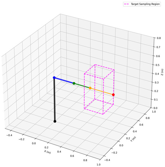
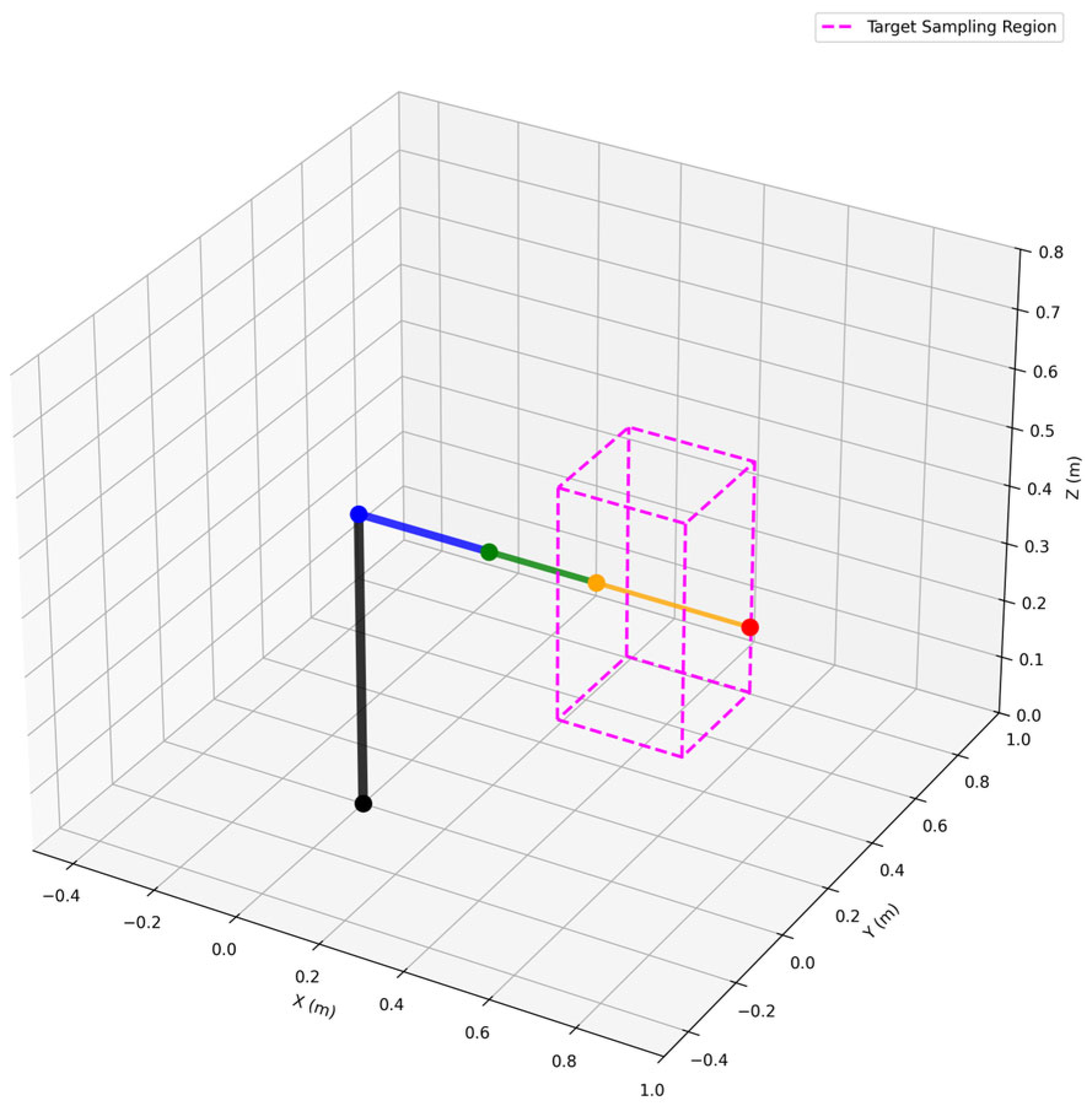
To validate the effectiveness and feasibility of the proposed SAC-SC framework on variable-configuration robotic arms, we conducted experiments in a simplified kinematic simulation environment built upon OpenAI Gym. This platform emulates a custom-designed four-degree-of-freedom (DoF) PRRR-type manipulator, whose mechanical configuration matches that of the physical hardware: one prismatic joint (P) along the z-axis and three revolute joints (R). The lengths of the last three links are manually adjustable prior to each task, thereby defining a parameterized configuration space. The simulated environment is illustrated in Figure 4, with the purple region indicating the target generation zone.

Figure 4. Simulation scenario for obstacle-free environment. The colored line segments represent different links of the robotic arm, with each color corresponding to a specific link length. The purple dashed cuboid denotes the target sampling region, within which the dynamic target is expected to appear.

Target points for grasping tasks were randomly sampled within the workspace defined by x ∈ [0.3, 0.6] m, y ∈ [0.3, 0.6] m, and z ∈ [0.1, 0.5] m. To ensure task feasibility, each generated target was verified for reachability using forward kinematics. The adjustable link lengths adhere to the Denavit–Hartenberg (DH) parameters of the real manipulator, as summarized in Table 3. During training initialization, all link lengths were set to their maximum values to maximize initial workspace coverage and facilitate policy exploration.

Table 3. Adjustable link length ranges for the PRRR manipulator.

Link ID	Min Length (m)	Max Length (m)
L1	0.1	0.5
L2	0.26	0.31
L3	0.2	0.25
L4	0.32	0.35

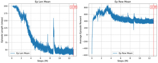
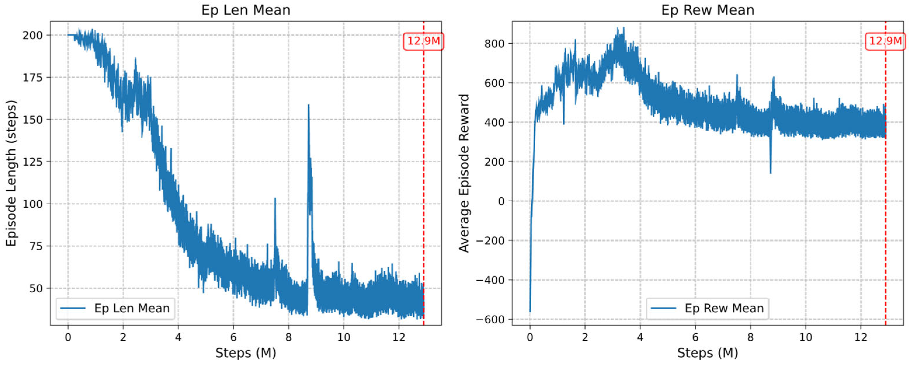
The SAC-SC framework employs the hybrid action space design introduced in Section 3. At the beginning of each episode, it outputs a set of link-length configurations; subsequently, it generates joint-angle increments in a continuous action space to complete trajectory planning. Training was carried out over approximately 30 million environmental interaction steps. To enhance training efficiency, a lightweight online evaluation mechanism was implemented: every 10,000 steps, the current policy was tested over 20 independent episodes. Training was terminated early if the task success rate reached 100% in five consecutive evaluations. A task was deemed successful if the Euclidean distance between the end-effector and the target point was less than 0.001 m, satisfying typical industrial positioning accuracy requirements. As shown in the convergence curves (Figure 5), the policy converged after approximately 12 million steps, evidenced by stabilization in both average episode length (left) and average reward per episode (right).

Figure 5. Training curves of the SAC-SC policy: episode length (left) and episode reward (right). The red dashed line marks the stopping point at 12.9 million steps, where the policy achieved 100% success rate in five consecutive evaluation rounds and the metrics stabilized.

For a comprehensive performance evaluation, three representative path planning baselines were selected:

• RRT (Rapidly exploring Random Tree Star): A probabilistically complete and asymptotically optimal sampling-based planner suitable for high-dimensional spaces and complex obstacle environments.
• Jacobian-IK: An iterative inverse kinematics (IK) solver based on the damped least squares (DLS) method applied to the Jacobian matrix, enhanced with multi-start initialization to improve robustness near singularities.
• Optimization-IK: Formulates IK as a constrained nonlinear least-squares problem with joint limits, solved via the SLSQP algorithm and augmented with multi-start search to mitigate local minima.

All methods were evaluated under identical conditions across 100 randomly generated single-target grasping scenarios, using the same success criterion and environment configuration.

Regarding the co-design of morphology and motion planning, it is important to note that the prevailing paradigm in existing co-design literature is a two-stage approach: an outer-loop evolutionary optimizer (commonly a Genetic Algorithm) searches over structural parameters, while an inner-loop planner evaluates task performance. Given the scarcity of end-to-end co-design methods for serial manipulators, this GA-based framework represents the de facto standard and most appropriate benchmark for our study.

Two sets of comparative experiments were designed:

• Trajectory Quality Validation: Fixing the link-length configuration output by SAC-SC, we compared the trajectories generated by SAC and the three baseline planners under the same kinematic structure.
• Joint Optimization Performance Comparison: SAC-SC was benchmarked against a two-stage optimization paradigm combining Genetic Algorithm (GA) with a path planner (“GA + Planner”).

Evaluation metrics included task success rate, end-effector positioning error, Cartesian path length, planning time, number of execution steps, joint motion as kinematic proxies for energy consumption, and configuration stability. All statistics are reported as mean ± standard deviation over 100 independent trials.

5.2. Trajectory Quality Validation

To assess the quality of trajectories generated by SAC-SC under a fixed configuration, we used the link-length setting produced by SAC-SC and compared SAC-SC’s policy against the three classical planners in an obstacle-free environment. Results are summarized in Table 4.

Table 4. Trajectory Quality Comparison in Fixed Configuration (Same Link Lengths).

Method	Success Rate (%)	Mean Error (m)	Path Length (m)	Planning Time (s)	Avg. Steps	Mean Total Joint Motion (Rad)	Mean Step-Wise Joint Motion (Rad/Step)
RRT*	97	0.0003 ± 0.0003	0.67 ± 0.10	0.372 ± 0.252	40.0 ± 9.6	1.0702 ± 0.2795	0.0267 ± 0.0020
Optimization-IK	100	0.0003 ± 0.0002	0.66 ± 0.10	0.002 ± 0.001	30.2 ± 7.8	1.0426 ± 0.2701	0.0346 ± 0.0014
Jacobian-IK	89	0.0046 ± 0.0151	0.66 ± 0.10	0.005 ± 0.002	42.5 ± 15.6	1.1466 ± 0.3166	0.0285 ± 0.0048
SAC-SC	100	0.0007 ± 0.0001	0.74 ± 0.12	0.027 ± 0.006	34.0 ± 7.2	1.2105 ± 0.3129	0.0352 ± 0.0025

Note: All results are based on 100 independent trials in a clutter-free environment with fixed link lengths. The success criterion is defined as end-effector-target distance < 0.001 m.

In terms of task success rate, both SAC-SC and Optimization-IK achieved 100%, significantly outperforming RRT* (97%) and Jacobian-IK (89%). Failures in RRT* stem from its probabilistic completeness—finite sampling may miss feasible paths in some instances—while Jacobian-IK suffers from numerical instability near kinematic singularities, leading to failure in approximately 11% of cases. In contrast, SAC-SC implicitly learns a feasible motion manifold through end-to-end policy training, demonstrating superior robustness.

Regarding computational efficiency, Optimization-IK requires only approximately 2 ms per query—over an order of magnitude faster than SAC-SC (approximately 27 ms). However, this speed relies heavily on an accurate kinematic model and a good initial guess, and crucially, Optimization-IK cannot participate in configuration selection. Although slower than analytical IK solvers, SAC-SC is still more than 10 times faster than RRT*, which exhibits a mean planning time exceeding 300 ms, meeting the real-time control requirements (30–50 Hz) of industrial robotic systems while supporting adaptive configuration.

In trajectory quality, SAC-SC achieves fewer execution steps (34.0) than RRT* (42.1) and Jacobian-IK (38.7), indicating a preference for concise, direct motion sequences. Its Cartesian path length (0.74 m) is slightly longer than that of Optimization-IK (0.66 m), which reflects a fundamental distinction: SAC-SC optimizes for task success and execution efficiency via learned policies, whereas traditional planners explicitly minimize geometric path length. To further assess motion efficiency—a key factor related to energy consumption—we report Mean Total Joint Motion and Mean Step-wise Joint Motion as kinematic proxies for actuation effort. SAC-SC exhibits a total joint motion of 1.2105 ± 0.3129 rad, only ~16% higher than Optimization-IK (1.0426 ± 0.2701 rad), and its per-step joint movement (0.0352 ± 0.0025 rad/step) is nearly identical to that of Optimization-IK (0.0346 ± 0.0014 rad/step). This demonstrates that SAC-SC implicitly learns smooth and energy-conscious trajectories comparable to specialized optimizers.

In summary, SAC-SC maintains high success rates and reasonable trajectory quality while offering strong generalization and deployment flexibility—laying a solid foundation for its integration into joint optimization tasks.

5.3. Obstacle-Free Joint Optimization Performance

To further evaluate SAC-SC’s capability in co-optimizing mechanism parameters and motion trajectories, we compared it against the conventional two-stage “GA + Planner” approach. In this baseline, the path planner is embedded within GA’s fitness function, with path length and execution steps as optimization objectives. Results in the obstacle-free setting are shown in Table 5. We selectgenetic algorithm (GA) as a representative of black-box, gradient-free optimization methods commonly used in early-stage robotic design. While not the most efficient, it serves as a conceptually simple baseline to highlight the paradigm shift enabled by our RL-based approach.

Table 5. End-to-End Joint Optimization Performance.

Method	Success Rate (%)	Mean Error (m)	Path Length (m)	Avg. Steps	Total Time per Task (s)	Mean Total Joint Motion (Rad)	Mean Step-Wise Joint Motion (Rad/Step)
GA + RRT*	100	0.0002 ± 0.0002	0.68 ± 0.10	40.4 ± 9.9	542.791	1.0857 ± 0.2911	0.0275 ± 0.0023
GA + Optimization-IK	100	0.0001 ± 0.0001	0.66 ± 0.10	29.7 ± 8.5	2.266	1.0408 ± 0.2800	0.0368 ± 0.0027
GA + Jacobian-IK	100	0.0001 ± 0.0000	0.67 ± 0.10	41.4 ± 16.0	6.596	1.1392 ± 0.3290	0.0306 ± 0.0072
SAC-SC	100	0.0007 ± 0.0001	0.74 ± 0.12	34.0 ± 7.2	0.145	1.2105 ± 0.3129	0.0363 ± 0.0025

Note: Total time includes both configuration search and trajectory planning. SAC-SC achieves real-time performance via end-to-end policy inference, while GA-based methods require iterative optimization over multiple generations. All tests conducted under identical conditions with 100 random targets.

SAC-SC achieves a per-task total runtime of only 0.145 s, which is approximately 15.6 times faster than the fastest GA variant (GA + Optimization-IK: 2.266 s) and more than 3700 times faster than GA + RRT* (approximately 540 s). This dramatic efficiency gain arises from a fundamental architectural difference: GA performs thousands of sequential simulations over 50 generations with 100 individuals per generation, making it impractical for online deployment; in contrast, SAC-SC encodes the entire joint optimization problem into a policy network during offline training, enabling end-to-end real-time decision-making via a single forward pass at inference time.

All methods achieve 100% success rate, confirming SAC-SC’s robustness. Its average end-effector error (0.7 mm) is slightly higher than GA methods (0.1–0.2 mm), attributable to SAC-SC’s use of sparse rewards that do not explicitly penalize small positioning deviations. Regarding energy-related performance, we evaluate Mean Total Joint Motion as a proxy for energy consumption. GA + Optimization-IK achieves the lowest value (1.0408 ± 0.2800 rad) due to its offline global optimization, while SAC-SC shows a modest increase (1.2105 ± 0.3129 rad, +16%). Crucially, the Mean Step-wise Joint Motion of SAC-SC (0.0363 ± 0.0025 rad/step) matches that of GA + Optimization-IK (0.0368 ± 0.0027 rad/step), confirming that the generated motions remain smooth and control-friendly. Path length and execution steps are comparable across methods, indicating that SAC-SC produces geometrically reasonable and motion-efficient trajectories.

Notably, SAC-SC reaches sub-millimeter accuracy after only 12 million training steps using a standard-sized policy network. Further improvements in precision can be achieved through: deeper or wider network architectures for enhanced function approximation; denser or hierarchical reward shaping for finer end-effector control; and curriculum learning or domain randomization to boost robustness, all without compromising its millisecond-level inference speed, highlighting the scalability advantage of learning-based approaches.

Moreover, statistical analysis of SAC-SC’s output link lengths (Table 6) reveals adaptive configuration behavior: l2 exhibits significant variation (standard deviation: 0.014 m), while l1 and l3 remain highly concentrated. This suggests the policy learns a task-aware strategy—adjusting l2 only when necessary—to maintain a stable, broadly capable default configuration. In contrast, GA shows minor but unstructured fluctuations across all links due to its stochastic mutation process, lacking clear task-driven intent. SAC-SC’s selective adaptation demonstrates its ability to internalize environmental structure and avoid redundant actuation.

Table 6. Stability Analysis of Link Length Selection.

Method	L1 (m)	L2 (m)	L3 (m)
GA + RRT*	0.265 ± 0.007	0.203 ± 0.005	0.326 ± 0.007
GA + OptIK	0.262 ± 0.005	0.201 ± 0.004	0.323 ± 0.006
GA + JacIK	0.263 ± 0.010	0.203 ± 0.009	0.324 ± 0.009
SAC-SC	0.260 ± 0.000	0.206 ± 0.014	0.321 ± 0.003

5.4. Obstacle-Aware Joint Optimization Performance

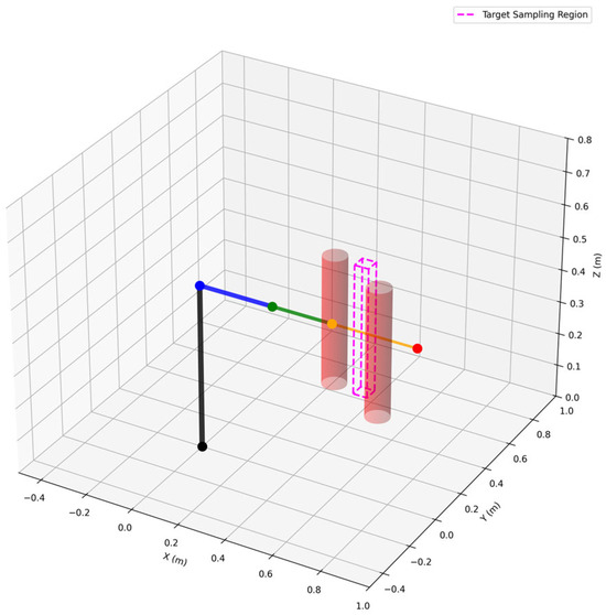
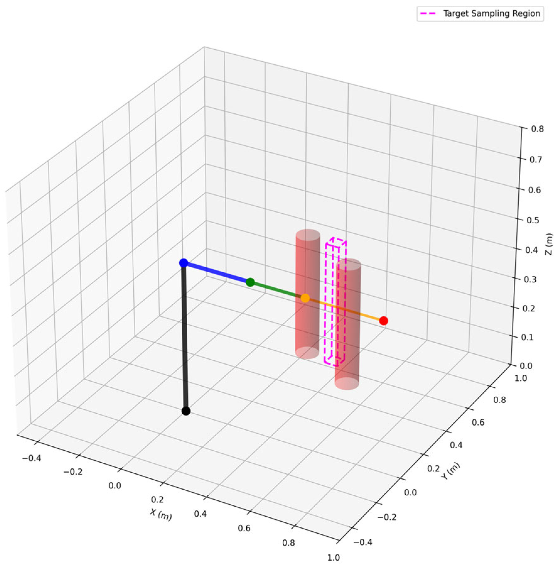
To evaluate SAC-SC under more realistic conditions, we introduced two static cylindrical obstacles (radius = 0.05 m) centered at [0.58, 0.32] m and [0.32, 0.45] m. Given the increased task complexity, the target region was narrowed to x,y ∈ [0.42, 0.48] m, z ∈ [0.1, 0.5] m to focus on a single feasible grasping pose. The scene is as shown in Figure 6. The reward function was augmented with a collision penalty (negative reward when obstacle distance < safety threshold), and the success criterion was relaxed to 0.01 m.

Figure 6. Simulation scenario for obstacle-aware environment. The red cylinders represent obstacles in the workspace, while the purple dashed region indicates the target sampling area for dynamic goals.

Since traditional IK solvers cannot handle obstacle avoidance, only two baselines were considered:

• RRT: Uses SAC-SC’s selected link lengths but relies solely on RRT for trajectory planning.
• GA + RRT: A two-stage method where GA first searches for optimal link lengths using Optimization-IK in free space (with path length and joint motion as fitness), followed by a single RRT* call for obstacle-avoidance trajectory—avoiding costly repeated RRT* evaluations inside GA.

Results (Table 7) show that SAC-SC achieves an 85.0% success rate, outperforming RRT* (73.0%) but slightly below GA + RRT* (95.0%). Importantly, this result was obtained without retraining or hyperparameter tuning for the obstacle-aware environment, suggesting untapped potential. With architectural enhancements (e.g., deeper networks), refined rewards, or curriculum learning, performance could be further improved.

Table 7. Performance Comparison in Obstacle-Aware Environment.

Metric	SAC-SC	RRT*	GA + RRT*
Success Rate (%)	85	73	95
Mean Error (m)	0.0159 ± 0.0182	0.0489 ± 0.0934	0.0028 ± 0.0026
Mean Path Length (m)	0.87 ± 0.07	0.80 ± 0.08	0.90 ± 0.10
Mean Planning Time (s)	0.070 ± 0.041	17.456 ± 7.583	18.154 ± 0.091
Mean Number of Steps	60.2 ± 8.7	68.7 ± 8.3	78.6 ± 11.1
Mean Total Joint Motion (rad)	1.9841 ± 0.1277	2.1335 ± 0.2616	2.4803 ± 0.3708
Mean Step-wise Joint Motion (rad/step)	0.0339 ± 0.0029	0.0310 ± 0.0011	0.0319 ± 0.0009

Note: The success criterion was relaxed to an end-effector-target distance < 0.01 m due to increased task complexity.

RRT*’s lower success stems from insufficient sampling in narrow passages, whereas SAC-SC implicitly learns a collision-avoidant motion manifold, yielding better adaptability. SAC-SC also achieves significantly lower positioning error (0.0159 ± 0.0182 m) than RRT* (0.0489 ± 0.0934 m), though GA + RRT* remains most accurate (0.0028 ± 0.0026 m) at high computational cost.

In path length, SAC-SC (0.87 ± 0.07 m) is slightly longer than RRT* (0.80 ± 0.08 m) but shorter than GA + RRT* (0.90 ± 0.10 m), reflecting a balanced trade-off between safety and efficiency. To further evaluate motion efficiency, we report Mean Total Joint Motion and Mean Step-wise Joint Motion as kinematic proxies for actuation effort. Notably, SAC-SC achieves the lowest total joint motion (1.9841 ± 0.1277 rad) among all methods, significantly lower than both RRT (2.1335 ± 0.2616 rad) and GA + RRT (2.4803 ± 0.3708 rad). Its mean step-wise joint motion (0.0339 ± 0.0029 rad/step) is also the smallest, indicating smoother and more controlled trajectories despite the presence of obstacles.

Most notably, SAC-SC’s planning time (0.070 ± 0.041 s) is approximately 250 times faster than both RRT*-based methods, and its average execution steps (60.2) are substantially fewer, enabling quicker task completion.

Thus, even in its current form, SAC-SC offers compelling advantages in real-time responsiveness, trajectory efficiency, and deployment simplicity. Critically, it does not rely on any specific planner or analytical model—instead, it learns joint decision-making from data, granting it strong generalization and adaptability. Future enhancements may include:

• Dynamic safety-margin-based reward shaping.
• Curriculum learning with gradually increasing obstacle complexity.
• Architectural extensions for better spatial reasoning.

These improvements would preserve SAC-SC’s millisecond inference latency while expanding its applicability to complex, real-world scenarios.

5.5. Cross-Simulation Generalization

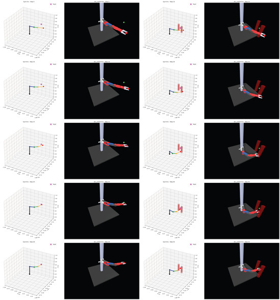
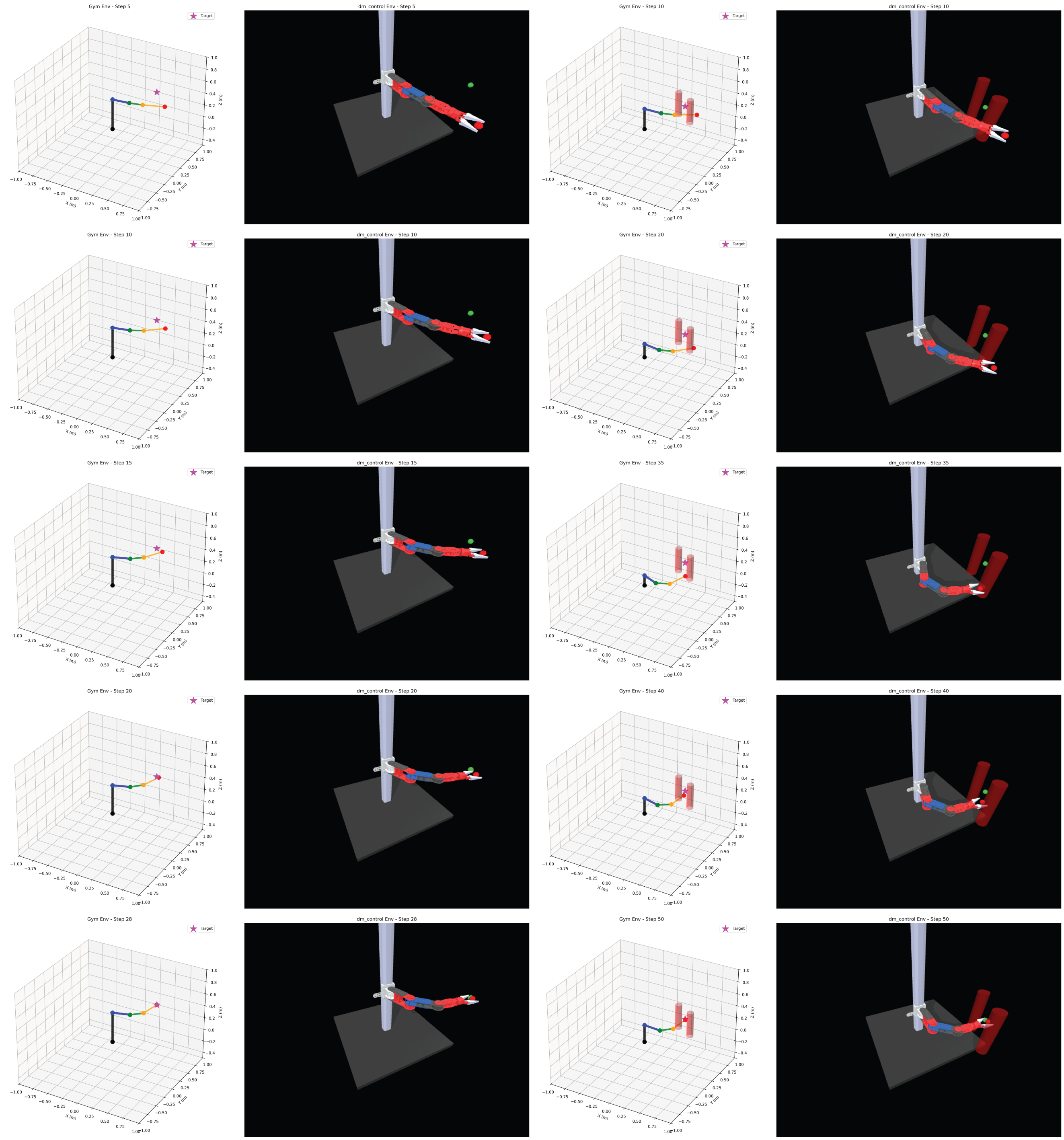
To assess robustness to modeling discrepancies, we performed zero-shot transfer: the policy trained solely in the simplified OpenAI Gym environment was directly deployed in a high-fidelity MuJoCo physics simulator (v3.3.2). The manipulator’s 3D model and kinematic parameters were defined in an XML-based MuJoCo scene file, which was loaded at simulation startup. The SAC-SC policy—implemented in Python—outputs target link lengths and joint angles; these values are passed directly to MuJoCo’s actuators via the dm_control interface during each control step. Both environments share identical nominal DH parameters. The SAC-SC outputs (link lengths and joint angles) were applied as open-loop control commands to MuJoCo actuators, mimicking real motor inputs. Targets were sampled from the original workspace, with 100 independent trials conducted. The result is shown in Figure 7 and Table 8.

Figure 7. Trajectory comparison between the simplified gym and high-fidelity simulator.

Table 8. End-Effector Positioning Accuracy in Zero-Shot Transfer Across Environments.

Scenario	RL Training Success Precision (m)	MuJoCo Simulation Error (m)
Obstacle-Free	0.001	0.0408 ± 0.0062
Obstacle-Aware	0.01	0.0342 ± 0.0102

The observed positioning error (~3 cm) in the MuJoCo environment is likely attributed to multiple sources of domain gap, including (1) unmodeled geometric details (e.g., motor housings, joint offsets), and (2) the absence of dynamic effects (e.g., inertia, friction) in the training environment. Since our policy was trained in a purely kinematic simulator, it outputs open-loop velocity commands that are sensitive to such mismatches. Nevertheless, the fact that the same structural configuration selected by SAC-SC remains effective in MuJoCo suggests the robustness of the high-level design decision.

Nevertheless, the manipulator consistently approached the target region without collisions or trajectory divergence, indicating that SAC-SC’s high-level decision logic, including configuration preference and motion direction, generalizes well across domains. This demonstrates structural robustness and validates its potential for Sim-to-Real transfer.

While open-loop transfer lacks the precision required for sub-millimeter industrial tasks, stable behavior in a physically realistic environment is promising. To bridge the fidelity gap, future work will train SAC-SC directly in high-fidelity simulators like MuJoCo. Despite higher per-step simulation costs, this “high-fidelity training to real-world deployment” paradigm is computationally feasible with parallel sampling and efficient RL algorithms, representing a viable path toward high-precision Sim-to-Real transfer.

5.6. Discussion

Collectively, our experiments reveal that SAC-SC achieves a pragmatic balance among real-time performance, robustness, and motion efficiency—rather than pursuing geometric or precision-based global optimality. In obstacle-free settings, it matches Optimization-IK with success rate (100%) and trajectory quality, while being more than 15 times faster than GA + Optimization-IK. In cluttered environments, it trades a modest 10% success deficit (85% versus 95%) for a reduction in planning time by a factor of over 260 and significantly fewer execution steps.

SAC-SC’s selective link-length adaptation reflects task-oriented reasoning, modifying configuration only when beneficial, thereby enhancing stability without sacrificing adaptability. In contrast, GA’s random search yields unstructured, low-amplitude fluctuations across all parameters.

We selected GA as the primary baseline because of its prevalence in engineering design and its ability to couple with arbitrary planners. “GA + Optimization-IK” represents a strong model-based upper bound. SAC-SC does not aim to surpass this theoretical optimum; rather, it demonstrates that near-optimal task performance can be achieved with drastically reduced computational overhead, making it suitable for dynamic, real-time applications.

The zero-shot transfer results further confirm that SAC-SC’s strategic decisions generalize across simulation domains, with performance degradation primarily due to unmodeled geometry, not policy failure. Retraining in high-fidelity environments is expected to resolve this.

Limitations include: the hybrid action space necessitates approximately 12 million training steps, significantly more than fixed-configuration RL; reward design for configuration selection relies on empirical priors, with performance highly sensitive to reward quality.

While the proposed SAC-SC framework demonstrates compelling performance in both simplified and high-fidelity simulation environments, its direct deployment on a physical reconfigurable manipulator would face several practical challenges rooted in the sim-to-real gap. These challenges merit explicit discussion as they define the boundary of the current work and inform future efforts.

First, the fidelity gap in environment modeling remains a fundamental barrier. Despite using MuJoCo for physics simulation, our training environment still relies on idealized assumptions about object geometry, surface friction, and contact dynamics. Constructing a digital twin that accurately captures real-world complexities—such as pose uncertainty due to sensor occlusion or subtle variations in workspace clutter—is a non-trivial engineering task. Policies trained under simplified conditions may fail when confronted with these unmodeled perturbations.

Second, unmodeled hardware imperfections in real actuators and sensors can significantly degrade performance. Our policy assumes precise execution of both joint angles and link lengths. However, real-world systems suffer from motor torque ripple, gear backlash, joint compliance, encoder noise, and control latency. Even small deviations in the realized morphology or motion trajectory can accumulate and lead to task failure.

Third, and most critically, our current RL formulation is kinematic-only, optimizing objectives such as end-effector error and path length without explicitly accounting for dynamic effects (e.g., inertia, Coriolis forces, or actuator torque limits). While this is acceptable in simulation, dynamically infeasible trajectories—especially those involving rapid morphological adaptation—may induce excessive vibration, tracking errors, or violation of motor constraints on a physical robot.

Addressing these gaps will be central to our future work, through approaches such as system identification for improved dynamic modeling, domain randomization to enhance policy robustness, and integration with low-level dynamic controllers to ensure feasible execution on hardware.

In conclusion, SAC-SC introduces a novel, efficient, and scalable paradigm for co-design in variable-configuration robots. Its core value lies not in replacing traditional optimization, but in providing a practical, deployable solution for scenarios demanding rapid response and operational flexibility—key requirements in modern robotic applications.

6. Conclusions

This study demonstrates that co-design of structural parameters and motion planning can be effectively realized within a unified reinforcement learning framework by treating continuous link lengths as part of the agent’s action space. The proposed SAC-SC method enables a reconfigurable PRRR manipulator to autonomously select task-adapted morphologies and execute collision-free trajectories in a single forward pass, without relying on external optimizers or differentiable simulators.

Empirical evaluation reveals that SAC-SC achieves consistent task success across both obstacle-free and cluttered environments, with inference times under 100 ms. Our method eliminates the need for iterative design-evaluation loops, enabling direct mapping from task specification to optimal configuration and control policy. Notably, the learned policy exhibits selective configuration behavior: it primarily adjusts the second link length when beneficial, while keeping other links stable, suggesting an emergent understanding of task-relevant kinematic trade-offs rather than exhaustive exploration.

However, this work has several limitations. First, the hybrid action space necessitates extensive training (~12 million steps), which is significantly more than fixed-configuration RL tasks. Second, the current reward function is handcrafted and task-specific; its performance is sensitive to the weighting of components like distance, progress, and collision penalty. Third, and most critically, our formulation is purely kinematic and ignores dynamic effects (e.g., inertia, torque limits), which may lead to dynamically infeasible trajectories on real hardware. Finally, the current implementation assumes static reconfiguration—link lengths are set once per episode and cannot adapt during task execution.

To address these limitations, we propose the following directions for future work.

• To reduce sample complexity, we will explore hierarchical RL or meta-learning frameworks that can transfer knowledge across tasks, thereby accelerating the learning of morphology-control co-adaptation.
• To generalize beyond handcrafted rewards, we will investigate inverse reinforcement learning (IRL) or preference-based learning to automatically infer reward functions from expert demonstrations or human feedback.
• To bridge the sim-to-real gap, we will train SAC-SC directly in high-fidelity physics engines (e.g., MuJoCo with accurate dynamics) and integrate it with low-level torque controllers to ensure dynamic feasibility.
• To enable online adaptation, we will extend the action space to support dynamic reconfiguration during task execution, provided the hardware supports rapid, safe morphological changes.

Zero-shot transfer from a simplified kinematic simulator to a high-fidelity MuJoCo environment confirms the robustness of the policy’s high-level decision logic, despite absolute positioning errors arising from unmodeled geometric details. This indicates strong potential for sim-to-real deployment when trained in physically accurate simulators. While SAC-SC does not guarantee globally optimal configurations in the traditional kinematic sense, it delivers near-optimal task performance with dramatically reduced computational overhead, making it particularly suitable for dynamic, real-time robotic applications where adaptability and speed outweigh theoretical optimality.

References

- Chen, Y.-L.; Cai, Y.-R.; Cheng, M.-Y. Vision-Based Robotic Object Grasping—A Deep Reinforcement Learning Approach. Machines 2023, 11, 275. [Google Scholar] [CrossRef] [Scilit]
- Pane, Y.P.; Nageshrao, S.P.; Kober, J.; Babuška, R. Reinforcement Learning Based Compensation Methods for Robot Manipulators. Eng. Appl. Artif. Intell. 2019, 78, 356–367. [Google Scholar] [CrossRef] [Scilit]
- Han, X.; Zhao, P.; Zhao, X.; Zi, B. Review on Machine Learning-Based Approaches for the Kinematic Analysis and Synthesis of Mechanisms. Front. Mech. Eng. 2025, 20, 11. [Google Scholar] [CrossRef] [Scilit]
- Gao, Z.; Zhang, D.; Ge, Y. Design Optimization of a Spatial Six Degree-of-Freedom Parallel Manipulator Based on Artificial Intelligence Approaches. Robot. Comput.-Integr. Manuf. 2010, 26, 180–189. [Google Scholar] [CrossRef] [Scilit]
- Wang, D.; Tan, D.; Liu, L. Particle Swarm Optimization Algorithm: An Overview. Soft Comput. 2018, 22, 387–408. [Google Scholar] [CrossRef] [Scilit]
- Peta, K.; Wiśniewski, M.; Kotarski, M.; Ciszak, O. Comparison of Single-Arm and Dual-Arm Collaborative Robots in Precision Assembly. Appl. Sci. 2025, 15, 2976. [Google Scholar] [CrossRef] [Scilit]
- Kuffner, J.J., Jr.; LaValle, S.M. RRT-Connect: An Efficient Approach to Single-Query Path Planning. In Proceedings of the 2000 IEEE International Conference on Robotics and Automation (ICRA), San Francisco, CA, USA, 24–28 April 2000; Volume 2, pp. 995–1001. [Google Scholar] [CrossRef] [Scilit]
- Tsianos, K.I.; Sucan, I.A.; Kavraki, L.E. Sampling-Based Robot Motion Planning: Towards Realistic Applications. Comput. Sci. Rev. 2007, 1, 2–11. [Google Scholar] [CrossRef] [Scilit]
- Daniel, K.; Nash, A.; Koenig, S.; Felner, A. Theta*: Any-Angle Path Planning on Grids. J. Artif. Intell. Res. 2010, 39, 533–579. [Google Scholar] [CrossRef] [Scilit]
- Lu, S.; Bingxiao, D.; Li, Y. Minimum-jerk trajectory planning pertaining to a translational 3-degree-of-freedom parallel manipulator through piecewise quintic polynomials interpolation. Adv. Mech. Eng. 2020, 12, 1–18. [Google Scholar] [CrossRef] [Scilit]
- Lillicrap, T.P.; Hunt, J.J.; Pritzel, A.; Heess, N.; Erez, T.; Tassa, Y.; Silver, D.; Wierstra, D. Continuous Control with Deep Reinforcement Learning. arXiv 2015, arXiv:1509.02971. [Google Scholar] [CrossRef] [Scilit]
- Haarnoja, T.; Zhou, A.; Hartikainen, K.; Tucker, G.; Ha, S.; Tan, J.; Kumar, V.; Zhu, H.; Gupta, A.; Abbeel, P.; et al. Soft Actor-Critic Algorithms and Applications. arXiv 2018, arXiv:1812.05905. [Google Scholar] [CrossRef] [Scilit]
- Kuo, P.-H.; Huang, C.-T.; Chang, C.-W.; Feng, P.-H.; Lin, Y.-S. Design and Implementation of a Soft Actor–Critic Controller for a Robotic Arm. Eng. Appl. Artif. Intell. 2025, 151, 110589. [Google Scholar] [CrossRef] [Scilit]
- Wang, Y.; Li, Z.; Zhao, X.; Wang, S.; Liu, H. Visual–Tactile Fusion and SAC-Based Learning for Robot Peg-in-Hole Assembly in Uncertain Environments. Machines 2025, 13, 605. [Google Scholar] [CrossRef] [Scilit]
- Chen, Y.; Su, S.; Ni, K.; Li, C. Integrated Intelligent Control of Redundant Degrees-of-Freedom Manipulators via the Fusion of Deep Reinforcement Learning and Forward Kinematics Models. Machines 2024, 12, 667. [Google Scholar] [CrossRef] [Scilit]
- Peters, D.L.; Papalambros, P.Y.; Ulsoy, A.G. Sequential Co-Design of an Artifact and Its Controller via Control Proxy Functions. Mechatronics 2013, 23, 409–418. [Google Scholar] [CrossRef] [Scilit]
- Fadini, G.; Flayols, T.; Del Prete, A.; Souères, P. Simulation Aided Co-Design for Robust Robot Optimization. IEEE Robot. Autom. Lett. 2022, 7, 11306–11312. [Google Scholar] [CrossRef] [Scilit]
- Schulman, J.; Wolski, F.; Dhariwal, P.; Radford, A.; Klimov, O. Proximal Policy Optimization Algorithms. arXiv 2017, arXiv:1707.06347. [Google Scholar] [CrossRef] [Scilit]
- Kubacki, A.; Adamek, M.; Baran, P. Analysis of Impact of Limb Segment Length Variations during Reinforcement Learning in Four-Legged Robot. Sci. Rep. 2024, 14, 27978. [Google Scholar] [CrossRef] [Scilit]
- Kitano, F.; Uchikata, H.; Matsusita, K.; Shiga, M.; Sasaki, M. Simultaneous Optimization of Mechanism and Control in Cooperative Work of Multiple Robot Arms. J. Jpn. Soc. AEM 2021, 29, 161–166. [Google Scholar] [CrossRef] [Scilit]
- Xu, J.; Chen, T.; Zlokapa, L.; Foshey, M.; Matusik, W.; Sueda, S.; Agrawal, P. An End-to-End Differentiable Framework for Contact-Aware Robot Design. arXiv 2021, arXiv:2107.07501. [Google Scholar] [CrossRef] [Scilit]
- Zhang, C.; Li, M.; Tong, W.; Huang, X. Morphology-Aware Graph Reinforcement Learning for Tensegrity Robot Locomotion. arXiv 2025, arXiv:2510.26067. [Google Scholar] [CrossRef] [Scilit]
Disclaimer/Publisher’s Note: The statements, opinions and data contained in all publications are solely those of the individual author(s) and contributor(s) and not of MDPI and/or the editor(s). MDPI and/or the editor(s) disclaim responsibility for any injury to people or property resulting from any ideas, methods, instructions or products referred to in the content. |
© 2026 by the authors. Licensee MDPI, Basel, Switzerland. This article is an open access article distributed under the terms and conditions of the Creative Commons Attribution (CC BY) license.