Modeling for Data Efficiency: System Identification as a Precursor to Reinforcement Learning for Nonlinear Systems

Abstract

Safe and sample-conscious controller synthesis for nonlinear dynamics benefits from reinforcement learning that exploits an explicit plant model. A nonlinear mass–spring–damper with hardening effects and hard stops is studied, and off-plant Q-learning is enabled using two data-driven surrogates: (i) a piecewise linear model assembled from operating region transfer function estimates and blended by triangular memberships and (ii) a global nonlinear autoregressive model with exogenous input constructed from past inputs and outputs. In unit step reference tracking on the true plant, the piecewise linear route yields lower error and reduced steady-state bias (MAE = $0.03$; SSE = $3\%$) compared with the NLARX route (MAE = $0.31$; SSE = $30\%$) in the reported configuration. The improved regulation is obtained at a higher identification cost (60,000 samples versus 12,000 samples), reflecting a fidelity–knowledge–data trade-off between localized linearization and global nonlinear regression. All reported performance metrics correspond to deterministic validation runs using fixed surrogate models and trained policies and are intended to support methodological comparison rather than statistical performance characterization. These results indicate that model-based Q-learning with identified surrogates enables off-plant policy training while containing experimental risk and that performance depends on modeling choices, state discretization, and reward shaping.

1. Introduction

The design of high-performance controllers traditionally relies on accurate mathematical models of system dynamics. When first-principles modeling is infeasible, system identification (SI) provides a suitable alternative, enabling the derivation of models directly from experimental data,  Keesman [1], Ljung [2], Landau and Zito [3], Chen et al. [4]. The scope of SI has expanded significantly, encompassing techniques for nonlinear,  Nelles [5], time-varying,  Majji et al. [6], and even unstable systems,  Kuo et al. [7], Pintelon and Schoukens [8], Lee et al. [9]. Identifying unstable systems presents a particular challenge, as open-loop operation risks damage or failure. Consequently, closed-loop SI methods have been developed, leveraging known controller dynamics to infer open-loop behavior, though often requiring considerable prior knowledge as discussed in  Huang et al. [10] and Chinvorarat et al. [11].

The advent of Deep Learning (DL) has further augmented SI, for instance, through multi-modal Long short-term memory (LSTM) networks for parameter estimation in uncertain systems,  Chiuso and Pillonetto [12], Cui et al. [13]. Concurrently, reinforcement learning (RL) has emerged as a promising paradigm for direct data-driven controller synthesis proposed in  Brunke et al. [14], Jaman et al. [15], Farheen et al. [16]. RL can address system modeling and control design simultaneously via model-based approaches or bypass modeling entirely in model-free frameworks proposed in  Chiuso and Pillonetto [12], Ross et al. [17], Martinsen et al. [18]. However, applying standard RL—often dependent on large amounts of exploratory interaction data—to unstable, safety-critical, or economically prohibitive physical systems remains a significant hurdle,  Shuprajhaa et al. [19], Hafner and Riedmiller [20].

This challenge has encouraged research into safer, more sample-efficient, data-driven control. Recent surveys, such as Martin et al. [21], catalog approaches such as semidefinite programming for nonlinear systems. Other methods integrate learning with robust control structures; for example, Gaussian Processes (GPs) learn safe regions for Model Predictive Control (MPC) parameters from experimental data, Airaldi et al. [22]. A two-stage methodology, which first estimates system parameters to bridge the simulation-to-reality gap, has also shown promise, as seen in applications for legged robots in Sobanbabu et al. [23].

For model-based RL, leveraging known or learned models during training to enhance safety and efficiency generally falls into three categories: (a) policy optimization-based approaches, which treat safety as a constrained cost minimization problem, Paternain et al. [24] and Chow et al. [25]; (b) control theory-based approaches, which embed safety through mathematical guarantees using tools such as Lyapunov functions, control barrier functions, or MPC in Berkenkamp et al. [26] and Cohen et al. [27]; and (c) formal methods-based approaches, which provide some level of verification against predefined safety specifications, Beard et al. [28] and Fulton et al. [29].

Building upon the two-stage philosophy, this paper conceptualizes two novel RL frameworks tailored for systems where extensive physical experimentation is dangerous, destructive, or prohibitively expensive. Both frameworks prioritize obtaining a reliable nonlinear model through SI before RL training. The first approach partitions the system’s operating range into regions where local linear models are identified; these are then fused into a global nonlinear representation using a fuzzy logic-based inference system. The second approach directly identifies a global nonlinear autoregressive model with exogenous inputs (NARX) from available data. In each case, the derived model serves as the environment for a subsequent RL agent to learn a control policy that meets closed-loop performance specifications.

The primary objective is to establish a practical pathway for the RL-based control of complex nonlinear systems. This work aims to provide a foundational methodology that can later be extended—utilizing specialized SI techniques for unstable systems—to the challenging domain of RL control for inherently unstable plants. Although tabular Q-learning does not explicitly require a process model, direct on-plant learning is impractical for nonlinear physical systems due to safety constraints, exploration cost, and actuator limits. In this work, system identification is employed to construct surrogate plant models that enable off-plant policy training within a model-based reinforcement learning framework. The identified models are not used to replace reinforcement learning but rather to provide a safe and sample-efficient environment for training Q-learning controllers prior to deployment on the true nonlinear plant.

The remainder of this paper is organized as follows. Section 2 reviews model-based reinforcement learning and tabular Q-learning. Section 3 presents the nonlinear mass–spring–damper plant and the system identification procedures used to construct the piecewise linear and NLARX surrogates, along with baseline approaches. Section 4 details the Q-learning training methodology, including state discretization, action design, and reward construction. Section 5 reports the closed-loop validation results on the true nonlinear plant and summarizes performance metrics. Section 6 discusses observed trade-offs, limitations, and implications. Section 7 concludes this paper and outlines prospective extensions.

2. Related Work

2.1. Model-Based Reinforcement Learning

Reinforcement learning (RL) enables an agent to learn control strategies by interacting with an environment and maximizing a cumulative notion of reward. Unlike model-free approaches, which rely solely on trial-and-error interaction, model-based reinforcement learning (MBRL) incorporates an explicit model of the environment to predict future state transitions and rewards as proposed in Sutton [30] and Moerland et al. [31]. This predictive capability allows planning to be interleaved with direct experience, thereby improving sample efficiency and control performance. The process flow in generic model-based reinforcement learning is depicted in Figure 1.

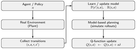
Figure 1. Process flow in model-based reinforcement learning.

A general model of the environment is characterized by the transition and reward mappings,

$$\mathcal{M}\triangleq \left(\mathbb{P}(s^{\prime }\mid s,a),\mathbb{R}(s,a)\right),$$

(1)

where $\mathbb{P}(s^{\prime }\mid s,a)$ represents the transition model that predicts the probability distribution of the next state $s^{\prime }$ given the current state s and action a, while $\mathbb{R}(s,a)$ denotes the expected reward associated with a state–action pair.

The use of such a model supports three fundamental aspects of MBRL:

1.

Model Learning: The estimation of the transition and reward models from interaction data, often through system identification, regression, or neural network approximation.

2.

Planning: The utilization of the learned model to simulate trajectories, enabling the agent to evaluate policies without direct environment interaction.

3.

Policy Optimization: Improvement in the policy or value function based on real and simulated experience.

The key optimization elements in model-based reinforcement learning include exploration strategies, model fidelity, sample efficiency, and stability and robustness. Exploration strategies, such as $ϵ$-greedy and upper confidence bound (UCB), are utilized to balance exploration and exploitation. In model fidelity, accurate predictions are ensured while avoiding overfitting to specific trajectories. Sample efficiency is observed when simulated rollouts reduce the demand for expensive real-environment interaction. Finally, stability and robustness are particularly important when approximations or nonlinearities are present.

MBRL algorithms may combine elements of both model-free and model-based reasoning. One widely adopted example is the Dyna architecture by Sutton [30], where real experience updates the model and value function directly, while additional planning steps use simulated experience generated from the model. Such integration allows the learning process to benefit from both data-driven accuracy and predictive foresight.

2.2. Q-Learning

Q-learning is a temporal difference control algorithm that learns an approximation of the optimal action value function $Q^{*}(s,a)$ without requiring a model of the environment as proposed in Watkins and Dayan [32]. Within an MBRL framework, Q-learning can be enhanced by using simulated experience to augment real interactions. The action value function is defined as

$$Q^{\pi }(s,a)=\mathbb{E}\left[\sum _{k=0}^{\infty }{\gamma }^k{r}_{t+k+1}|s_t=s,a_t=a,\pi \right],$$

(2)

where $\pi$ is the policy; $\gamma \in [0,1)$ is the discount factor; $s_t,a_t,$ and $r_t$ are state, action, and reward values at the current time stamp, respectively; and $r_{t+k+1}$ is the reward received $k+1$ steps into the future.

Q-learning employs an off-policy scheme, meaning that the policy used to select actions (the behavior policy) may differ from the policy being improved (the target policy). In practice, an $ϵ$-greedy strategy is often adopted for exploration, while updates always aim at the greedy (optimal) policy. This separation enables the learning of the optimal value function independently of the current exploration strategy. The algorithm uses temporal difference (TD) learning, which updates value estimates by bootstrapping from subsequent predictions. The TD error is defined as

$${\delta }_t=r_{t+1}+\gamma \underset{a^{\prime }}{max}Q(s_{t+1},a^{\prime })-Q(s_t,a_t).$$

(3)

The update rule for Q-learning is then given by

$$Q(s_t,a_t)\leftarrow Q(s_t,a_t)+\alpha {\delta }_t,$$

(4)

where $\alpha \in (0,1]$ is the learning rate. This update occurs at every time step, enabling the online refinement of value estimates.

The pseudo-code for Q-learning is summarized as follows (Algorithm 1):

Algorithm 1 Q-learning Algorithm.

1: Initialize $Q(s,a)$ arbitrarily for all states s and actions a 2: for each episode do 3:       Initialize starting state s 4:       for each step in the episode do 5:             Select action a using $ϵ$-greedy policy from $Q(s,:)$ 6:             Execute action a, observe reward r and next state $s^{\prime }$ 7:             Compute TD error: $\delta =r+\gamma {max}_{a^{\prime }}Q(s^{\prime },a^{\prime })-Q(s,a)$ 8:             Update value: $Q(s,a)\leftarrow Q(s,a)+\alpha \delta$ 9:             Set $s\leftarrow s^{\prime }$ 10:       end for 11: end for

By integrating Q-learning into the MBRL setting, the learned model can generate synthetic transitions $(s,a,r,s^{\prime })$ to further update the Q-function. This hybrid approach leverages the stability of temporal difference learning while exploiting the predictive capability of the environment model, improving efficiency in complex nonlinear control tasks.

3. Approach

The proposed model-based reinforcement learning framework for nonlinear dynamics is designed for a virtual mass–spring–damper system (NL-MSD) with nonlinear characteristics, treated as a true system.

3.1. Mass–Spring–Damper Dynamics with Hardening Nonlinearity

Let $x\left(t\right)$ denote position and $v\left(t\right)=\dot{x}\left(t\right)$ velocity. The input $u\left(t\right)$ takes values from a finite set $\mathcal{U}=\{-F,-\frac{F}{2},0,\frac{F}{2},F\}$, where $F>0$ denotes a fixed force magnitude. The admissible position range is $x\left(t\right)\in [-L/2,L/2]$ with $L=5$, i.e., $x\in [-2.5,2.5]$. At the range boundaries, velocity is forced to zero to emulate hard stops.

The continuous-time model has a mass $m>0$, viscous damping coefficient $c>0$, linear spring gain $k>0$, sinusoidal spring gain parameter $g>0$, and a cubic hardening coefficient $h>0$, and the force balance reads

$$m\ddot{x}\left(t\right)=u\left(t\right)-c\dot{x}\left(t\right)-ksin\left(gx\left(t\right)\right)-h{x}^3\left(t\right).$$

(5)

The boundary constraint (hard stops) defines the admissible set $\mathcal{X}=[-L/2,L/2]$. The state constraint enforces

$$x\left(t\right)\in \mathcal{X}\mathrm{for}\mathrm{all}t,\mathrm{and}\mathrm{if}x\left(t\right)\in \{\pm L/2\}\mathrm{with}\mathrm{outward}\mathrm{velocity},\mathrm{then}\dot{x}\left(t\right)=0.$$

(6)

In practice, this is implemented by saturating x to $\mathcal{X}$ and zeroing the velocity at the boundaries.

The discrete-time Euler form has a sampling time $\mathsf{\Delta }t=0.01\mathrm{s}$ and the state $z_k={\left[\begin{array}{cc}{x}_k& v_k\end{array}\right]}^{\top }$, and a forward-Euler step yields

$$\begin{array}{cc}\hfill v_{k+1}& =v_k+{\displaystyle \frac{\mathsf{\Delta }t}{m}}\left(u_k-c{v}_k-ksin\left(g{x}_k\right)-h{x}_k^3\right),\hfill \end{array}$$

(7a)

$$\begin{array}{cc}\hfill {\tilde{x}}_{k+1}& =x_k+\mathsf{\Delta }t{v}_{k+1},\hfill \end{array}$$

(7b)

$$\begin{array}{cc}\hfill x_{k+1}& ={\mathrm{proj}}_{[-L/2,L/2]}\left({\tilde{x}}_{k+1}\right),\hfill \end{array}$$

(7c)

$$\begin{array}{cc}\hfill & \mathrm{if}{x}_{k+1}\in \{\pm L/2\}\mathrm{and}({\tilde{x}}_{k+1}\notin [-L/2,L/2]),\mathrm{set}{v}_{k+1}\leftarrow 0,\hfill \end{array}$$

(7d)

where ${\mathrm{proj}}_{\mathcal{X}}(·)$ denotes Euclidean projection onto $\mathcal{X}$.

The action set or the input $u_k$ at each step results from a discrete action $a_k\in \{1,2,3,4,5\}$ via

$$a_k\in \{1,2,3,4,5\}⟹u_k\in \{-F,-\frac{F}{2},0,\frac{F}{2},F\},$$

(8)

with a fixed $F>0$ chosen for the experiment. An additive bias B may be included if required by the test condition.

Two modeling strategies are considered for approximating the system dynamics and enabling reinforcement learning control, as depicted in Figure 2. Model constructions utilizing the proposed steps are detailed in the following sections.

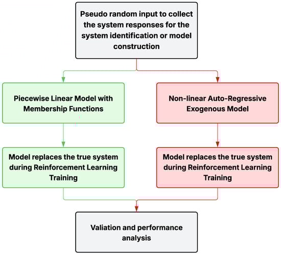
Figure 2. Process flow of MBRL experiments.

3.2. Piecewise Linear Model (PLM) with Membership Functions

Section 3.4.1 presents a single global linear model as a baseline to illustrate the limitations of conventional linear identification when applied to nonlinear dynamics. This model serves as a reference point for evaluating the necessity and effectiveness of the proposed piecewise linear and nonlinear surrogate modeling approaches. A data-driven surrogate is constructed by identifying five local linear models around bias points $B\in \{-10,-5,0,5,10\}\mathrm{N}$. Around each bias, an input $u\left(t\right)=B+\upsilon \left(t\right)$ is applied, where $\upsilon \left(t\right)$ takes pseudo-random values in $\{\pm 1\}\mathrm{N}$ so that the total force toggles in a small neighborhood of the selected bias while exciting the plant dynamics. Each experiment records $12,000$ input–output samples at sampling time $\mathsf{\Delta }t=0.01$ s around a specified bias; the measured output is position $x\left(t\right)$, and the applied input is the force $u\left(t\right)$, as assembled into an identification dataset object. This experiment was repeated for all the bias levels independently to form the local linear models.

Continuous-time identification and discretization processes are carried out for each bias data record, and a second-order transfer function model is estimated using tfest (System Identification Toolbox, MATLAB^® (https://www.mathworks.com/products/matlab.html)). The continuous-time second-order model is then discretized at $\mathsf{\Delta }t=0.01$ s. The resulting discrete numerator/denominator polynomials are stored for each bias case (N1,...,N5) and (D1,...,D5), and the fit is visualized as shown in Figure 3 to report the goodness of fit. The goodness of fit is measured for each identified model, and validation quality is reported as the Best-Fit percentage. The metric is defined as

$$\mathrm{Fit}=\left(1-{\displaystyle \frac{\parallel y-\widehat{y}{\parallel }_2}{\parallel y-\overline{y}{\parallel }_2}}\right)\times 100\%,$$

(9)

where y is the measured output, $\widehat{y}$ is the model-predicted output, and $\overline{y}$ denotes the mean of the measured output. A fit of $100\%$ indicates a perfect reproduction of the data, whereas $0\%$ or negative values indicate that the model performs no better (or worse) than the mean response. After discretization, each per-bias discrete model $G_i\left(z\right)$ (index $i=1,\dots ,5$ for $B\in \{-10,-5,0,5,10\}$) is represented in the z-domain as

$$G_i\left(z\right)={\displaystyle \frac{n_{i,1}{z}^{-1}+n_{i,2}{z}^{-2}}{1+d_{i,1}{z}^{-1}+d_{i,2}{z}^{-2}}},\mathsf{\Delta }t=0.01\mathrm{s},$$

(10)

which induces the recursion

$$y_i\left[k\right]=n_{i,1}u[k-1]+n_{i,2}u[k-2]-d_{i,1}{y}_i[k-1]-d_{i,2}{y}_i[k-2],$$

(11)

where u is the measured force input, and $y_i$ is the model output.

Figure 3. Piecewise linear model validation at selected biases including the fitting metric.

Stitching the local model output to create a global model via triangular membership weighting is conducted at run time, and the five local model outputs $\left\{y_i\left[k\right]\right\}$ are blended with non-negative weights $\left\{w_i\right\}$ that satisfy ${\sum }_i{w}_i>0$, yielding the stitched surrogate output

$$\widehat{x}\left[k\right]={\displaystyle \frac{{\sum }_{i=1}^5{w}_i\left({\xi }_k\right)y_i\left[k\right]}{{\sum }_{i=1}^5{w}_i\left({\xi }_k\right)}}.$$

(12)

The weights are triangular membership functions of a scheduling variable ${\xi }_k$ (position-related state), realized as piecewise linear functions $f_1,\dots ,f_5$ that activate over overlapping ranges and are zero elsewhere. The membership function follows the following definitions (13):

$$\begin{array}{cc}\hfill f_1\left(x\right)& =\left\{\begin{array}{cc}1,\hfill & x<-2,\hfill \\ -(x+1),\hfill & -2\le x\le -1,\hfill \\ 0,\hfill & \mathrm{otherwise},\hfill \end{array}\right.\hfill \end{array}$$

(13a)

$$\begin{array}{cc}\hfill f_2\left(x\right)& =\left\{\begin{array}{cc}0,\hfill & x<-1.5,\hfill \\ 2(x+1.5),\hfill & -1.5\le x\le -1.0,\hfill \\ -2(x+0.5),\hfill & -1.0<x\le -0.5,\hfill \\ 0,\hfill & \mathrm{otherwise},\hfill \end{array}\right.\hfill \end{array}$$

(13b)

$$\begin{array}{cc}\hfill f_3\left(x\right)& =\left\{\begin{array}{cc}0,\hfill & x<-1,\hfill \\ x+1,\hfill & -1\le x\le 0,\hfill \\ -(x-1),\hfill & 0<x\le 1,\hfill \\ 0,\hfill & \mathrm{otherwise},\hfill \end{array}\right.\hfill \end{array}$$

(13c)

$$\begin{array}{cc}\hfill f_4\left(x\right)& =\left\{\begin{array}{cc}0,\hfill & x<0.5,\hfill \\ 2(x-0.5),\hfill & 0.5\le x\le 1,\hfill \\ -2(x-1.5),\hfill & 1<x\le 1.5,\hfill \\ 0,\hfill & \mathrm{otherwise},\hfill \end{array}\right.\hfill \end{array}$$

(13d)

$$\begin{array}{cc}\hfill f_5\left(x\right)& =\left\{\begin{array}{cc}0,\hfill & x<1,\hfill \\ 2(x-1),\hfill & 1\le x\le 1.5,\hfill \\ 1,\hfill & x>1.5.\hfill \end{array}\right.\hfill \end{array}$$

(13e)

as encoded in the membership routine. In the stitched simulator, each local output is computed from its discrete coefficients $(N_i,D_i)$ as

$$y_i\left[k\right]=\left(N_i(2:)\right)U[k-1:k-2]-\left(D_i(2:)\right)Y[k-1:k-2],$$

(14)

and the final surrogate $\widehat{x}\left[k\right]$ is produced by (12).

3.3. Nonlinear Autoregressive Exogenous (NLARX)

A single, global surrogate is constructed by learning a nonlinear autoregressive model with exogenous input (NLARX) from input–output data generated by the true mass–spring–damper with nonlinearity (MSD-NL) plant. The excitation consists of a pseudo-random force sequence switching among $\{-F,-\frac{F}{2},0,\frac{F}{2},F\}$ with $F=10\mathrm{N}$, yielding an input range of $[-10,10]\mathrm{N}$. A record of $\mathrm{12,000}$ samples is acquired at sampling time $\mathsf{\Delta }t=0.01\mathrm{s}$ by driving the true nonlinear plant and logging the position response; the minimum dwell times and the total horizon are selected so that the switching signal adequately excites the dynamics while preserving bounded operation. The data preparation used here (sample count, sampling time, action set, and pseudo-random switching with dwell limits) is not optimized for the experiments.

Let $x_k\in \mathbb{R}$ denote the measured position at discrete time k and $u_k\in \mathbb{R}$ the applied force. A second-order regressor is employed with two past outputs and two past inputs with a one-step input transport delay:

$${\varphi }_k={\left[\begin{array}{cccc}{x}_{k-1}& x_{k-2}& u_{k-1}& u_{k-2}\end{array}\right]}^{\top },\mathsf{\Delta }t=0.01\mathrm{s}.$$

(15)

The NLARX mapping takes the form

$$x_k=F_{\theta }\left({\varphi }_k\right)+e_k,$$

(16)

where $F_{\theta }:{\mathbb{R}}^4\to \mathbb{R}$ is a static nonlinear function parameterized by $\theta$, and $e_k$ denotes the one-step prediction error. In this study, $F_{\theta }$ is chosen as a shallow feedforward mapping with sigmoidal basis units,

$$F_{\theta }\left(\varphi \right)=c_0+\sum _{j=1}^S{\alpha }_j\sigma \left({\beta }_j^{\top }\varphi +{\beta }_{0j}\right),$$

(17)

with parameters $\theta ={\{c_0,{\alpha }_j,{\beta }_j,{\beta }_{0j}\}}_{j=1}^S$ and $\sigma (·)$ a logistic sigmoid. This structure corresponds to a second-order NLARX (two output lags, two input lags, one-step input delay) driven by the regressor (15).

The identification proceeds by minimizing the one-step prediction error on the collected record under mild regularization to prevent overfitting. After learning, the surrogate is validated on the same excitation profile by computing the predicted position ${\widehat{x}}_k=F_{\theta }\left({\varphi }_k\right)$ and by reporting the normalized Best-Fit percentage against the measured $x_k$ (definition given in the piecewise model subsection). A representative validation plot for the NLARX model is shown in Figure 4, which displays the measured true response and the model prediction over the validation samples.

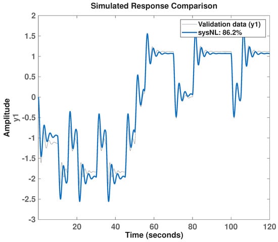
Figure 4. NLARX model validation including fitting metric.

Compared with the single global linear model in Section 3.4.1, the nonlinear autoregressive model in Section 3.3 improves prediction fidelity over a broader operating range by incorporating past input–output histories. While the global fit remains imperfect, the increased model expressiveness provides a more informative surrogate for reinforcement learning than a single linear approximation.

3.4. Baseline Models

To strengthen the comparative analysis, additional baseline model identification and model-based reinforcement learning (MBRL) strategies are examined. These include (i) a single global linear model used directly within the MBRL loop, (ii) the Dyna–Q algorithm as a planning-based MBRL method, and (iii) a principled justification for selecting five linear segments in the piecewise linear modeling (PLM) framework.

3.4.1. Global Linear Model (GLM) Identification

A global linear approximation of the nonlinear plant is first identified under the assumption that the system order is known. Transfer function estimation is applied to the training dataset generated from pseudo-random exploration. The resulting model exhibits approximately $86\%$ fit on the validation data, as shown in Figure 5. This linear model replaces the true nonlinear plant within the MBRL loop for 300 episodes, each consisting of 3000 decision steps including other experimental setup parameters, as described in Section 4.

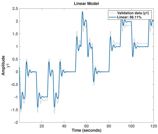
Figure 5. Model fit profile of globally identified linear model.

The Q-table evolution obtained from interaction with the linear surrogate is shown in Figure 6a. A structured state–action pattern emerges, suggesting that the agent develops a directional policy toward the desirable region of the state space. When the learned agent is evaluated on the true nonlinear plant, however, the resulting steady-state output remains approximately $66\%$ below the target reference, as illustrated in Figure 6b. This indicates that the mismatch between the global linear approximation and the nonlinear dynamics significantly limits policy transferability.

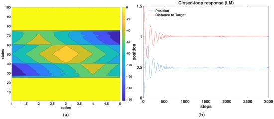
Figure 6. (a) Q-table evolution over 300 episodes for the global linear model, and (b) the closed-loop validation of the learned agent on the true plant, showing a $66\%$ steady-state error.

3.4.2. Dyna–Q with Planning

The Dyna–Q algorithm is evaluated using a planning step size of 100 while keeping the episode configuration identical to the linear-model-based MBRL. Because the algorithm performs direct plant interactions in addition to simulated planning steps, the cumulative real-system interaction increases substantially, reducing the benefit of model-based substitution.

The Q-table obtained after 300 episodes is shown in Figure 7a. The emerging patterns indicate the progressive formation of a meaningful state–action profile. Nevertheless, validation on the true system again settles roughly $66\%$ below the desired steady-state value, as displayed in Figure 7b. This behavior parallels the performance of the single linear model and highlights insufficient model fidelity within the learning process.

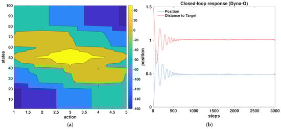
Figure 7. (a) Q-table evolution after 300 episodes for the Dyna–Q algorithm with planning size 100, and (b) the closed-loop validation of the learned Dyna–Q agent on the true plant. The output settles approximately $66\%$ below the target.

3.4.3. The Rationale Behind the Number of Segments Selected in the PLM Framework

The five linear models used in the PLM framework are locally identified operating region models and are distinct from the single global linear model presented in Section 3.4.1. These local models are combined through membership-based blending to form the proposed piecewise linear surrogate.

In the piecewise linear modeling approach, the nonlinear spring force term is partitioned into multiple linear segments by assigning a constant stiffness parameter K within each region. The mean absolute error (MAE) between the linearized force approximation and the true nonlinear force is used as the criterion for determining the number of segments. Because the force nonlinearity intensifies with displacement, increased segmentation generally reduces the MAE. However, excessive segmentation introduces unnecessary model complexity and reduces interpretability.

The plant under study tolerates a maximum allowable MAE of 5 (force units). A sweep over candidate segment counts indicates that the minimal number achieving acceptable accuracy is five, which yields an MAE of approximately $4.2$. The force comparison between the true nonlinear model and the five-segment approximation is presented in Figure 8. Subsequent identification, model learning, and MBRL-based control procedures for the PLM approach proceed as already described earlier in this manuscript.

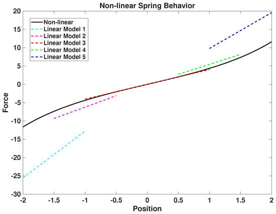
Figure 8. Comparison between true nonlinear force and five-segment piecewise linear approximation.

4. Methodology

The objective centers on training a discrete action agent by Q-learning while bypassing the true plant and employing a single model per study (either the stitched piecewise linear model or the NLARX model). Training proceeds for $N_{\mathrm{ep}}=300$ episodes with $T=3000$ steps per episode; the Q-table is initialized to all zeros and stored across episodes for the visualization of learning progress (surface maps). Episodes are simulated at a sampling time of $\Delta t=0.01$ s with a force alphabet of five actions $\{-F,-\frac{F}{2},0,\frac{F}{2},F\}$; unless noted, $F=10$ N.

The state design (error-indexed discretization) is constructed as follows. Let $x_k$ denote the position at time step k and $x^{★}$ the target position. The raw tracking error is $e_k=x_k-x^{★}$, with clipping to the admissible interval $[e_{min},e_{max}]=[-5,5]$ that reflects the $\pm 2.5$ unit position range. A 100-state grid is formed by the scaling of the clipped error to indices $s_k\in \{1,\dots ,100\}$:

$${\tilde{e}}_k=max\left(e_{min},min(e_{max},e_k)\right),s_k=1+\mathrm{round}\left({\displaystyle \frac{(N_s-1)({\tilde{e}}_k-e_{min})}{e_{max}-e_{min}}}\right),N_s=100.$$

(18)

State $s=50$ corresponds to zero error and is the most desirable operating point. The discretization resolution of $N_s=100$ states represents a compromise between error resolution near the setpoint and tractable Q-table size for tabular learning. Finer grids reduce quantization error but increase sample complexity and slow convergence, whereas coarser grids limit achievable steady-state accuracy. The selected resolution is found to be sufficient to capture the dominant closed-loop behavior for the present bounded-error regulation task. A systematic sensitivity study with alternative grid resolutions is beyond the scope of this work.

At each step, the agent selects one of the five actions. The action determines a force in $\{-F,-\frac{F}{2},0,\frac{F}{2},F\}$ applied to the surrogate model for state propagation. The scalar reward combines a term that depends on the absolute error and a term that depends on the change in absolute error between consecutive steps. Let $E_k=\left|e_k\right|$ and $\Delta E_k=E_k-E_{k-1}$. With two positive scalars g and $\zeta$ and the normalization $E_{max}=e_{max}=5$, the instantaneous reward reads

$$r_k=g{\displaystyle \frac{1}{1+E_k}}-\zeta {\displaystyle \frac{\mathsf{\Delta }{E}_k}{E_{max}}},$$

(19)

so that smaller error and decreases in error are rewarded, while increases in error are penalized. The weighting parameters g and $\zeta$ in the reward definition are selected heuristically to balance steady-state accuracy and transient improvement while maintaining bounded reward magnitudes over the admissible error range. The normalization by $E_{max}$ ensures comparable scaling between the absolute error and error reduction terms. These parameters are not optimized through cross-validation, as the focus of this study is on surrogate model fidelity rather than reward tuning. The sensitivity of closed-loop behavior to reward weighting is acknowledged but remains outside the present scope. Equation (19) matches the plotted surface (reward as a function of $\left|e\right|$ and $\mathsf{\Delta }\left|e\right|$), as shown in Figure 9, and the individual penalty and fitness function plots are shown in Figure 10. In training, the decrement term is realized by a finite difference in the absolute error tracked over time, with normalization by the error range as follows:

$$\Delta E_k=|e_k|-|e_{k-1}|,\mathrm{use}-{\displaystyle \frac{\Delta E_k}{e_{max}-e_{min}}}\mathrm{as}\mathrm{the}\mathrm{signed}\mathrm{improvement}\mathrm{signal}.$$

(20)

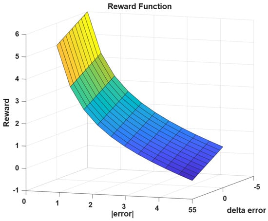
Figure 9. The reward function utilized in the MBRL process.

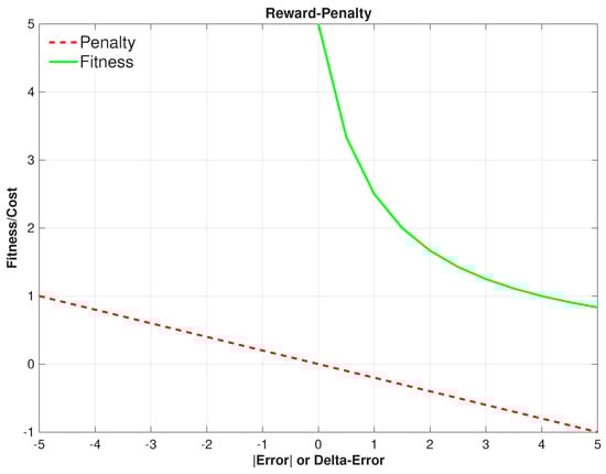
Figure 10. The reward and penalty elements utilized in the reward function construction.

Action selection follows $ϵ$-greedy exploration with exploration probability $ϵ$; the typical values used are $\alpha =0.5$ (learning rate), $\gamma =0.9$ (discount), $ϵ=0.1$ (exploration), and a scalar gain $A>0$ to scale the reward (reward amplification). The Q-update at step k is

$$Q(s_k,a_k)\leftarrow Q(s_k,a_k)+\alpha \left(A{r}_k+\gamma \underset{a^{\prime }}{max}Q(s_{k+1},a^{\prime })-Q(s_k,a_k)\right)+\eta \varphi (s_k,a_k),$$

(21)

where $\varphi (s,a)\le 0$ is a bounded shaping term that mildly penalizes actions incompatible with the coarse state region, and $\eta >0$ is its weight. This auxiliary term biases learning toward consistent actuation while preserving the Bellman target in the bracketed expression.

At the start of training $Q\equiv 0$; a full tensor of Q-tables across episodes is retained for offline visualization. Unless otherwise specified, episodes begin from rest ($x_0=0$; $v_0=0$), and the target position is drawn within the admissible range to expose the agent to a variety of setpoint locations; the state index is derived from the clipped error by (18). During training, the surrogate model exclusively advances the state. For the stitched piecewise model, five second-order local recursions are run in parallel and blended by triangular membership weights to produce the next predicted position; the resulting error is mapped to the next state by (18). For the NLARX model, the next predicted position is obtained by evaluating the nonlinear mapping on the regressor of two past outputs and inputs, with a one-step input delay; the predicted position then yields the next discrete state via (18). In both cases, no direct interaction with the true plant occurs during Q-learning rollouts. The Q-table progress as a heat map is created, as depicted in Figure 11 and Figure 12, for the PLM and NLARX, respectively. Filled contour plots of the Q-table illustrate how the value function evolves from the initial pre-convergence Q-function to the final convergence.

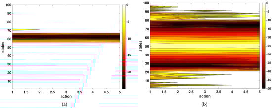
Figure 11. Q-table learning status for PLM: (a) at beginning (after single episode) and (b) end of all episodes.

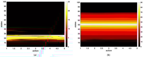
Figure 12. Q-table learning status for NLARX: (a) at beginning (after single episode) and (b) end of all episodes.

5. Performance Analysis

Closed-loop validation is conducted on the true nonlinear mass–spring–damper system after training the Q-learning agent with one of the two data-driven models (piecewise linear model, PLM, or nonlinear autoregressive model with exogenous input, NLARX). Each validation run consists of a single episode of length $T=3000$ steps with sampling time $\mathsf{\Delta }t=0.01$ s. The reference input is a unit position, $x^{★}=1$, and the goal is to drive the measured position $x_k$ to $x^{★}$ rapidly with small transient deviation and minimal bias. The trained Q-table is held fixed during validation. Representative position responses under the two trained agents are shown in Figure 13. In each plot, the measured position and the absolute tracking error $e_k=x_k-x^{★}$ are displayed to highlight convergence, transient behavior, and steady-state bias.

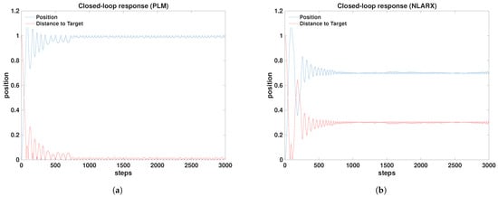
Figure 13. Controller validation and closed-loop system response to the unit reference: (a) tested with the trained agent from the PLM-MBRL, showing the closed-loop response obtained using the piecewise linear surrogate composed of the five locally identified linear models, and (b) tested with the trained agent from the NLARX-MBRL.

The performance metrics are considered as follows. Let $e_k=x_k-x^{★}$ denote the tracking error and $N=T$ the number of validation samples. The mean absolute error (MAE) and the standard deviation of the error (STD) are defined as $\mathrm{MAE}={\displaystyle \frac{1}{N}}{\sum }_{k=1}^N\left|e_k\right|,$ $\mathrm{STD}=\sqrt{{\displaystyle \frac{1}{N-1}}{\sum }_{k=1}^N{\left(e_k-\mathrm{MAE}\right)}^2}$. For a unit step reference, percent overshoot (PO) and settling time ($t_s$) are defined in the standard way:

$$\mathrm{PO}[\%]=100{\displaystyle \frac{{max}_k{x}_k-x^{★}}{|x^{★}|}},t_s=min\left\{k\mathsf{\Delta }t:|e_j|\le \epsilon |x^{★}|\forall j\ge k\right\},$$

(22)

with $\epsilon =0.02$ unless stated otherwise. The steady-state error (SSE) is evaluated over a terminal window $\mathcal{W}$ and reported as a percentage of the reference magnitude, $\mathrm{SSE}[\%]=100{\displaystyle \frac{\left|\frac{1}{\left|\mathcal{W}\right|}{\sum }_{k\in \mathcal{W}}{e}_k\right|}{|x^{★}|}}$.

The principal validation metrics for the two trained agents are summarized in Table 1. Training sample counts refer to the data used to construct the respective data-driven model prior to Q-learning. All reported closed-loop metrics correspond to deterministic validation runs using a fixed surrogate model and a fixed initial condition. Once the identified model and trained Q-table are fixed, the resulting closed-loop response is repeatable and does not exhibit stochastic variability. Consequently, performance comparisons are based on the reported MAE, standard deviation, steady-state error, overshoot, and settling time rather than on ensemble statistics across multiple trials.

Table 1. Closed-loop performance metrics on the true system for a unit reference ($x^{★}=1$). Settling time and overshoot are reported as N/A for the GLM and Dyna–Q cases because the closed-loop responses exhibit large steady-state bias and do not enter the prescribed $\pm 2\%$ tolerance band around the reference, rendering standard settling time and overshoot definitions inapplicable.

Model	MAE	STD	SSE [%]	Overshoot [%]	Settling Time [s]	Training Samples
NLARX	0.31	0.09	30	12	7	12,000
PLM	0.03	0.10	3	10	7	60,000
GLM	1.01	0.07	66	N/A	7	12,000
Dyna-Q	1.01	0.07	66	N/A	7	N/A

For the global linear model and the Dyna–Q baseline, the persistent steady-state error prevents convergence to the reference within the specified tolerance, and therefore settling time and percent overshoot are not defined for these cases. The PLM-trained agent exhibits a markedly lower mean absolute error and substantially lower steady-state error relative to the NLARX-trained agent, indicating superior bias rejection around the unit setpoint and overall tighter tracking. Percent overshoot is slightly smaller for the PLM case, while the settling time is identical at approximately 7 s for both agents under the stated criterion. The standard deviation of the error is comparable across the two cases, reflecting similar residual fluctuations about the final value once the transient decays. From a data perspective, the PLM approach aggregates $60,000$ samples via five operating point experiments to populate local linear dynamics across the range, whereas the NLARX approach relies on a single $12,000$-sample experiment spanning the full input range, which results in a more compact data requirement but a larger steady-state bias in the reported validation. In qualitative terms, the desired performance consists of low overshoot, short settling time, and minimal steady-state bias while maintaining low error overall and modest training cost. The PLM results align more closely with these goals at the expense of larger identification data; the NLARX results illustrate a faster data collection phase but increased bias and mean error in the tested scenario. This trade-off underscores the fact that piecewise local linearization over a grid of operating conditions can yield high-fidelity behavior near the reference at the cost of multiple experiments, whereas a single global nonlinear regression reduces identification effort but may underfit key nonlinearities or exhibit bias under the tested reference transition.

6. Discussion

The results indicate that both data-driven models enable the off-plant training of a discrete action agent that achieves closed-loop tracking on the true nonlinear mass–spring–damper system. The piecewise linear model (PLM) yields a lower mean absolute error and substantially reduced steady-state bias relative to the nonlinear autoregressive model with exogenous input (NLARX), at comparable overshoot and settling time. This behavior suggests that locally valid linear descriptions, blended across the operating range with fuzzy membership attributes, provide an effective basis for value iteration in the present task when the validation reference is a unit step.

A central trade-off emerges between prior knowledge and data demands. The construction of the PLM presupposes decisions about model order and about the placement of operating biases at which local models are identified. Such design choices encode valuable prior information about the plant, but this information is not always available for complex nonlinear systems or may be costly to obtain. In contrast, the NLARX route requires less a priori structure and concentrates data collection in a single experiment spanning the full input range. The observed increase in the mean and steady-state error for the NLARX-trained agent reflects the well-known tension between model generality and bias: a compact global regressor fitted on a heterogeneous dataset may underrepresent the regimes most relevant to the validation target, whereas locally fitted linear models emphasize fidelity near their operating regions. This comparison highlights that approaches requiring minimal existing knowledge are attractive and also challenging, particularly where safety or actuation limits restrict exploratory richness.

Several aspects of the learning formulation influence the reported performance. The discrete 100-state error index imposes a quantization of the value function that bounds achievable accuracy near the setpoint; finer partitions reduce quantization error but increase sample complexity. The five-action alphabet constrains the closed-loop authority and contributes to the observed overshoot; richer action sets reduce actuation quantization at the cost of a larger Q-table. The reward combines absolute error and its one-step change; this choice accelerates transient improvement yet can amplify sensitivity to short-horizon variability when the prediction model is imperfect. The hard stop projection at the position limits ensures safety but introduces kinks in the closed-loop map; trajectories that graze the boundary can therefore exhibit non-smooth value updates, which the tabulated metrics do not fully reveal.

The fidelity gap between the identified model used for training and the true plant used for validation constitutes a primary source of residual bias. For the PLM, model mismatch is dominated by interpolation across membership regions and by unmodeled cross-coupling between regimes; careful placement and shaping of the membership functions mitigate these effects. For NLARX, mismatch arises from regressor under-parameterization, choice of basis nonlinearity, and distributional differences between training and validation trajectories. Both models generalize from pseudo-random excitation to reference tracking, but the distribution shift from exploration to a deterministic setpoint task contributes to the steady-state deviations observed for the global model.

From a computational perspective, both models are light-weight at run time: the PLM requires the update of a small number of second-order recursions and a convex combination, while NLARX evaluation reduces to a static nonlinear map on a short regressor. The primary cost lies in data collection and model fitting, which is higher for the PLM due to multiple operating point experiments but lower for NLARX due to a single broad-range experiment. The reported outcomes therefore present complementary pathways: when modest prior knowledge about order and operating regions is available, PLM-based training delivers superior bias rejection; when such knowledge is scarce or the plant is difficult to segment, an NLARX-based route reduces up-front design effort at the expense of increased steady-state error in the present configuration.

A statistical characterization across randomized initial conditions or repeated training trials is not pursued in this study. The primary objective is a methodological comparison of surrogate modeling strategies for off-plant reinforcement learning rather than probabilistic performance assessment, which is left for future work. The reported validation fit percentages correspond to open-loop prediction under pseudo-random excitation and are not used as acceptance criteria for closed-loop control performance. For reinforcement learning-based regulation, local fidelity near the operating region is more critical than global prediction accuracy, and moderate open-loop fit can still yield effective policies when combined with error-based state representation. This study remains subject to limitations. Performance is quantified for a unit step target; multi-step or trajectory tracking, disturbance rejection, and robustness to unmodeled friction changes merit separate assessment. The use of model-bypassed rollouts mitigates experimental risk but introduces model-induced bias in the learned value surface, which suggests examining online model adaptation or intermittently grounded updates with limited true-plant interaction. Finally, the discretized state–action setting provides clarity and stability for tabular learning but does not exploit the potential smoothness of the value function; continuous approximators with constrained exploration may reduce quantization artifacts while preserving safety.

7. Conclusions

This study demonstrates that model-based reinforcement learning augmented with data-driven system identification enables off-plant policy training for nonlinear regulation while limiting experimental risk. A nonlinear mass–spring–damper system with hardening effects and hard stops is addressed using two surrogate modeling strategies: a piecewise linear model constructed from operating region identifications and a global nonlinear autoregressive model with exogenous input learned from a single broad-range experiment. Tabular Q-learning on an error-indexed state space with a finite force alphabet produces stabilizing controllers that achieve reference tracking on the true plant. The results highlight a fidelity–knowledge–data trade-off: locally identified and blended linear models provide tighter regulation and reduced steady-state bias when operating region knowledge is available, whereas global nonlinear regression reduces identification effort at the cost of increased residual error in the tested configuration. The adopted discretization and reward structure are shown to be effective and transparent for analysis while remaining modular and transferable to other bounded actuation systems. Future extensions include the adaptive refinement of the state partition, uncertainty-aware planning within the model loop, and limited on-plant fine-tuning to mitigate model–plant mismatch while preserving safety.

References

- Keesman, K.J. System Identification: An Introduction; Springer: Berlin/Heidelberg, Germany, 2011. [Google Scholar]
- Ljung, L. System Identification. In Signal Analysis and Prediction; Birkhäuser Boston: Boston, MA, USA, 1998; pp. 163–173. [Google Scholar]
- Landau, I.D.; Zito, G. Digital Control Systems: Design, Identification and Implementation; Springer: London, UK, 2006. [Google Scholar]
- Chen, C.W.; Huang, J.K.; Phan, M.; Juang, J.N. Integrated System Identification and State Estimation for Control of Flexible Space Structures. J. Guid. Control. Dyn. 1992, 15, 88–95. [Google Scholar]
- Nelles, O. Nonlinear System Identification. Meas. Sci. Technol. 2002, 13, 646. [Google Scholar] [CrossRef]
- Majji, M.; Juang, J.N.; Junkins, J.L. Observer/Kalman-Filter Time-Varying System Identification. J. Guid. Control Dyn. 2010, 33, 887–900. [Google Scholar]
- Kuo, C.H.; Schoen, M.P.; Chinvorarat, S.; Huang, J.K. Closed-Loop System Identification by Residual Whitening. J. Guid. Control Dyn. 2000, 23, 406–411. [Google Scholar] [CrossRef]
- Pintelon, R.; Schoukens, J. System Identification: A Frequency Domain Approach; Wiley: Hoboken, NJ, USA, 2012. [Google Scholar]
- Lee, H.; Huang, J.K.; Hsiao, M.H. Frequency Domain Closed-Loop System Identification with Known Feedback Dynamics. In Proceedings of the AIAA Guidance, Navigation, and Control Conference; AIAA: Reston, VA, USA, 1995. [Google Scholar]
- Huang, J.K.; Lee, H.C.; Schoen, M.P.; Hsiao, M.H. State-Space System Identification from Closed-Loop Frequency Response Data. J. Guid. Control Dyn. 1996, 19, 1378–1380. [Google Scholar]
- Chinvorarat, S.; Lu, B.; Huang, J.K.; Schoen, M.P. Setpoint Tracking Predictive Control by System Identification Approach. In Proceedings of the 1999 American Control Conference; IEEE: Piscataway, NJ, USA, 1999; Volume 1, pp. 331–335. [Google Scholar]
- Chiuso, A.; Pillonetto, G. System Identification: A Machine Learning Perspective. Annu. Rev. Control. Robot. Auton. Syst. 2019, 2, 281–304. [Google Scholar] [CrossRef]
- Cui, M.; Khodayar, M.; Chen, C.; Wang, X.; Zhang, Y.; Khodayar, M.E. Deep Learning-Based Time-Varying Parameter Identification for System-Wide Load Modeling. IEEE Trans. Smart Grid 2019, 10, 6102–6114. [Google Scholar]
- Brunke, L.; Greeff, M.; Hall, A.W.; Yuan, Z.; Zhou, S.; Panerati, J.; Schoellig, A.P. Safe Learning in Robotics: From Learning-Based Control to Safe Reinforcement Learning. Annu. Rev. Control. Robot. Auton. Syst. 2022, 5, 411–444. [Google Scholar] [CrossRef]
- Jaman, G.G.; Monson, A.; Chowdhury, K.R.; Schoen, M.; Walters, T. System Identification and Machine Learning Model Construction for Reinforcement Learning Control Strategies Applied to LENS System. In Proceedings of the 2022 Intermountain Engineering, Technology and Computing (IETC); IEEE: Piscataway, NJ, USA, 2022; pp. 1–6. [Google Scholar] [CrossRef]
- Farheen, N.; Jaman, G.G.; Schoen, M.P. Model-Based Reinforcement Learning with System Identification and Fuzzy Reward. In Proceedings of the 2024 Intermountain Engineering, Technology and Computing (IETC); IEEE: Piscataway, NJ, USA, 2024; pp. 80–85. [Google Scholar] [CrossRef]
- Ross, S.; Bagnell, J.A. Agnostic System Identification for Model-Based Reinforcement Learning. arXiv 2012, arXiv:1203.1007. [Google Scholar] [CrossRef]
- Martinsen, A.B.; Lekkas, A.M.; Gros, S. Combining System Identification with Reinforcement Learning-Based MPC. IFAC-PapersOnLine 2020, 53, 8130–8135. [Google Scholar] [CrossRef]
- Shuprajhaa, T.; Sujit, S.K.; Srinivasan, K. Reinforcement Learning-Based Adaptive PID Controller Design for Control of Linear/Nonlinear Unstable Processes. Appl. Soft Comput. 2022, 128, 109450. [Google Scholar]
- Hafner, R.; Riedmiller, M. Reinforcement Learning in Feedback Control: Challenges and Benchmarks from Technical Process Control. Mach. Learn. 2011, 84, 137–169. [Google Scholar] [CrossRef]
- Martin, T.; Schön, T.B.; Allgöwer, F. Guarantees for data-driven control of nonlinear systems using semidefinite programming: A survey. Annu. Rev. Control 2023, 56, 100911. [Google Scholar] [CrossRef]
- Airaldi, F.; De Schutter, B.; Dabiri, A. Learning safety in model-based reinforcement learning using MPC and Gaussian processes. IFAC-PapersOnLine 2023, 56, 5759–5764. [Google Scholar] [CrossRef]
- Sobanbabu, N.; He, G.; He, T.; Yang, Y.; Shi, G. Sampling-based system identification with active exploration for legged robot sim2real learning. arXiv 2025, arXiv:2505.14266. [Google Scholar]
- Paternain, S.; Chamon, L.; Calvo-Fullana, M.; Ribeiro, A. Constrained reinforcement learning has zero duality gap. In Proceedings of the Advances in Neural Information Processing Systems; Neural Information Processing Systems Foundation: La Jolla, CA, USA, 2019; Volume 32. [Google Scholar]
- Chow, Y.; Ghavamzadeh, M.; Janson, L.; Pavone, M. Risk-constrained reinforcement learning with percentile risk criteria. J. Mach. Learn. Res. 2018, 18, 1–51. [Google Scholar]
- Berkenkamp, F.; Turchetta, M.; Schoellig, A.; Krause, A. Safe model-based reinforcement learning with stability guarantees. In Proceedings of the Advances in Neural Information Processing Systems; Neural Information Processing Systems Foundation: La Jolla, CA, USA, 2017; Volume 30. [Google Scholar]
- Cohen, M.H.; Belta, C. Safe exploration in model-based reinforcement learning using control barrier functions. Automatica 2023, 147, 110684. [Google Scholar]
- Beard, J.J.; Baheri, A. Safety verification of autonomous systems: A multi-fidelity reinforcement learning approach. arXiv 2022, arXiv:2203.03451. [Google Scholar]
- Fulton, N.; Platzer, A. Safe reinforcement learning via formal methods: Toward safe control through proof and learning. In Proceedings of the AAAI Conference on Artificial Intelligence; AAAI: Washington, DC, USA, 2018; Volume 32. [Google Scholar]
- Sutton, R.S. Dyna, an integrated architecture for learning, planning, and reacting. ACM SIGART Bull. 1991, 2, 160–163. [Google Scholar] [CrossRef]
- Moerland, T.M.; Broekens, J.; Jonker, C.M. Model-based Reinforcement Learning: A Survey. Found. Trends Mach. Learn. 2023, 16, 1–118. [Google Scholar] [CrossRef]
- Watkins, C.J.; Dayan, P. Q-learning. Mach. Learn. 1992, 8, 279–292. [Google Scholar] [CrossRef]
Disclaimer/Publisher’s Note: The statements, opinions and data contained in all publications are solely those of the individual author(s) and contributor(s) and not of MDPI and/or the editor(s). MDPI and/or the editor(s) disclaim responsibility for any injury to people or property resulting from any ideas, methods, instructions or products referred to in the content. |
© 2026 by the authors. Licensee MDPI, Basel, Switzerland. This article is an open access article distributed under the terms and conditions of the Creative Commons Attribution (CC BY) license.